Article

Can a Hierarchical Classification of Sentinel-2 Data Improve Land Cover Mapping?

by
Adam Waśniewski
1,2,*,
Agata Hościło
1 and
Milena Chmielewska
1
1
Centre of Applied Geomatics, Institute of Geodesy and Cartography, Modzelewskiego 27, 02-679 Warsaw, Poland
2
Department of Geoinformatics, Cartography and Remote Sensing, Faculty of Geography and Regional Studies, University of Warsaw, Krakowskie Przedmieście 30, 00-927 Warsaw, Poland
*
Author to whom correspondence should be addressed.
Remote Sens. 2022, 14(4), 989; https://doi.org/10.3390/rs14040989
Submission received: 10 January 2022 / Revised: 3 February 2022 / Accepted: 16 February 2022 / Published: 17 February 2022
(This article belongs to the Special Issue European Remote Sensing-New Solutions for Science and Practice)

Abstract

:
Monitoring of land cover plays an important role in effective environmental management, assessment of natural resources, environmental protection, urban planning and sustainable development. Increasing demand for accurate and repeatable information on land cover and land cover changes causes rapid development of the advanced, machine learning algorithms dedicated to land cover mapping using satellite images. Free and open access to Sentinel-2 data, characterized with high spatial and temporal resolution, increased the potential to map and to monitor land surface with high accuracy and frequency. Despite a considerable number of approaches towards land cover classification based on satellite data, there is still a challenge to clearly separate complex land cover classes, for example grasslands, arable land and wetlands. The aim of this study is to examine, whether a hierarchal classification of Sentinel-2 data can improve the accuracy of land cover mapping and delineation of complex land cover classes. The study is conducted in the Lodz Province, in central Poland. The pixel-based land cover classification is carried out using the machine learning Random Forest (RF) algorithm, based on a time series of Sentinel-2 imagery acquired in 2020. The following nine land cover classes are mapped: sealed surfaces, woodland broadleaved, woodland coniferous, shrubs, permanent herbaceous (grassy cover), periodically herbaceous (i.e., arable land), mosses, non-vegetated (bare soil) and water bodies. The land cover classification is conducted following two approaches: (1) flat, where all land cover classes are classified together, and (2) hierarchical, where the stratification is applied to first separate the most stable land cover classes and then classifying the most problematic once. The national databases served as the source of the reference sampling plots for the classification process. The process of selection and verification of the reference sampling plots is performed automatically. To assess the stability of the classification models the classification processes are performed iteratively. The results of this study confirmed that the hierarchical approach gave more accurate results compared to the commonly used flat approach. The median of the overall accuracy (OA) of the hierarchical classification was higher by 3–9 percentage points compared to the flat one. Of interest, the OA of the hierarchical classification reached 0.93–0.99, whereas the flat approach reached 0.90. Individual classes are also better classified in the hierarchical approach.

1. Introduction

Growing population, urban sprawl, changes in land cover and land use result in an increased need for systematic and accurate land cover and land use information [1]. Highly accurate information on land cover and land use is essential for decision makers, urban planners [2], mapping of ecosystem services [3], deforestation analysis [4], detection of land cover changes [5], and many others. Satellite imagery are recognized as one of the most important data source for land cover mapping [6,7], monitoring the dynamics of the land cover changes at local, regional, national and global scales [8,9,10,11].
Since the launch of the Landsat’s satellite mission, rapid development of the image processing and analysis has been observed [12]. It results in the development of land cover classification methods, which have evolved substantially over the last four decades [13]. Several studies successfully applied a set of Landsat data for land cover analysis in urban environments [13], forestry [14,15,16,17], agriculture [18] or wetlands [13].
Nowadays, the Sentinel-2 data are more frequently used in the land cover classification domain [19]. This is due to the shorter revisit frequency compared to Landsat, higher spatial resolution—10 m compared to 30 m for Landsat, wider swath—290 km compared to 185 km of Landsat [20]. Additionally, the Sentinel-2 offers three red edge bands particularly useful for distinguishing the vegetation classification [21,22]. Red edge bands of Sentinel-2 data have been recognized as important variables, for example, for forest type mapping using a random forest classifier [15,16,23]. Forkour et al. [23] demonstrated that adding red edge bands of Sentinel-2 to the Landsat-8 bands resulted in increasing the OA of land cover classification from 0.90 to 0.92 and Kappa coefficient from 0.88 to 0.90.
A review of the application of Sentinel-2 in land cover mapping by Phiri et al. [24] confirmed the advantage of the Sentinel-2 data compared to the Landsat data for land cover mapping, especially in the urban domain, crop fields mapping, forests and water resources monitoring. The authors stressed, in particular, the advantage of machine learning algorithms applied in the classification processes. They concluded, based on literature review, that the land cover classifiaction of Sentinel-2 data using mashine learning provides high accuracies, higher than 0.80. Furthermore, the high and temporal spatial resolution and wide swath of the Sentinel-2 mission allows observing and monitoring of the rapid changes in ecosystems and human activities at the global scale with high detail. World Cover is the one of the latest global land cover products derived based on a synergy of Sentinel-1 and Sentinel-2 data acquired in 2020, by the European Space Agency (ESA) [25]. It consists of eleven land cover classes mapped at a 10 m spatial resolution. The OA of this global product is equal to 0.74. The highest user’s (UA) and producer’s accuracy (PA) were obtained for the tree cover, snow/ice, permanent water bodies, and bare/spare vegetation classes, reaching more than 0.80. The most problematic classes, with the lowest UA and PA values of around 0.50, are wetlands, shrubs, and moss/lichen classes [25]. Another example of the global land cover map derived based on Sentinel-2 data is the ESRI 2020 Land Cover map [26]. The OA of this map was equal to 0.86. The map was produced using a deep learning model trained with over 5 billion hand-labelled Sentinel-2 pixels from 20,000 sites all over the World. Out of 10 land cover classes, the highest UA and PA, above 0.82, was achieved for the classes representing water, trees and built-up areas. The classes such as grass, flooded vegetation, shrubs and bare ground achieved the lowest accuracy between 0.38 and 0.73, indicating that these classes are the most difficult to delineate [26].
Sentinel-2 data have also been used to derive pan-European land cover maps. One example is the Land Cover Map for Europe 2017 developed by the Space Research Centre of Polish Academy of Science as a result of the S2 Global Land Cover project [27]. The authors used the Random Forest method to classify 13 land cover classes with the OA equal to 0.86. The water bodies, coniferous and broadleaved tree cover classes were recognized as the more accurately classified classes with the PA and UA of 0.95–0.97. The lowest UA and PA values (0.10 to 0.50) were obtained for the permanent snow, marshes, moors and heathland classes, respectively [27]. The Sentinel-2 land cover product over Europe will be shortly delivered as part of the Copernicus Land Monitoring Service (CLMS). The European Environment Agency (EEA), responsible for implementation of CLMS has started to develop a new series of land cover products called CLC+, supported by the EAGLE data model, which is also hierarchical [28]. The new generation of the CLC+ product will contain the CLC+ Backbone, CLC+ Core and CLC+ instances components [29]. The CLC+ Backbone component will provide a detailed wall to wall vector and raster land cover layer with basic 12 land cover classes for raster products derived based on the classification of Sentinel-2 data.
In the last decade, the rapid development of Earth Observation technologies has been observed, both in terms of technological progress in new sensors as well as in development of advanced methods of data processing and analysis. The development of artificial intelligence, machine learning algorithms and access to high computing facilitates reduced the processing time and allows more efficient processing and analysis of the Big Data. The most popular machine learning algorithms applied for land cover analyses are RFs [30], Support Vector Machines (SVM) [31] and Convolution Neural Networks (CNN) [32]. Several studies have focused on selection of the best algorithms for land cover classification. Jamali [33] evaluated and compared eight machine learning models: RF, Decision Table, DTNB, J48, Lazy IBK, Multilayer Perceptron (MLPC), Non-Nested Generalized Exemplars (NNge), and Simple Logistic for land use/land cover mapping over the Sari region (Iran) using Landsat 8 OLI. The authors pointed out the NNge, followed by Lazy IBK, RF and MLPC as the best algorithms for accurate land cover mapping [33]. Noi et al. [34] compared RF, SVM and k-nearest neighbour (kNN) algorithms for land cover classification based on Sentinel-2 data in the north of the Red River Delta in Vietnam. All three algorithms gave comparable OA values: kNN 0.94., RF 0.94 and SVM 0.95 [35]. Amani et al. [35] reported that the RF classifier reached higher accuracy than SVM, kNN, Decision Tree (DT), Maximum Likelihood (ML) in the classification of wetland areas in Canada, based on Landsat-8, Sentinel-1 and elevation data. By contrast, a study by Dabija et al. [36] showed that the land cover classification with SVM reached higher OA compared to RF in land cover classification of Braila, Catalonia and Warsaw regions, 0.86 and 0.80, respectively. Inglada et al. [37] compared RF, SVM, decision tree and stochastic gradient boosting (SGB) algorithms in crop mapping in 12 regions located in 12 countries. They demonstrated that the RF reached higher accuracy for eight regions compared to SVM (difference of 5 to 20 percentage points), in the remining four regions the accuracy was on the same level. The superiority of the RF algorithm over other classifiers for land cover classification was also confirmed by Adam et al. [38]. The classification accuracy dependents on many factors such as the number of reference samples [39], number of land cover classes [36] or different satellite data. The RF classifier is less sensitive to tuning parameters compared to other algorithms [22]. It allows combination of different variable types, for example categorical and continuous data [40]. Rodriguez-Galiano et al. [41] highlighted the following advantages of an RF classifier in land cover mapping: (a) it works well on large datasets, (b) can handle thousands of inputs, (c) estimates the variable importance in the classification process, and (d) generates an internal objective generalization error. Additionally, the RF is relatively robust to noise and outliers, and it is computationally lighter and less time consuming than other machine learning approaches.
Mapping land cover with Sentinel-2 data using an RF algorithm is very popular with different scales and locations. Usually, the classification is carried out in a standard flat approach, where all land cover classes are classified together at the same time. The OA is provided as one value for the final product and, even though it achieves a relatively high value, the final product is not always high quality considering the spatial variability of different land cover classes. Beside the long heritage of land cover classification using remote sensed techniques, there are still classes that are challenging to separate [42]. Nguyen et al. [39] classified Sentinel-2 images into 11 land cover classes in Dag Nong Province (Vietnam), and pointed out the classes representing the plantation, croplands and residential areas as the most problematic and difficult to separate (PA ranged from 0.33 to 0.46) [39]. A study by Ghorbanian et al. [43] stressed that the wetland class is the most challenging class for delineating using Sentinel-2 imagery in Iran. Among the 13 land cover classes, wetlands reached the lowest PA and UA values of 0.89 and 0.86, respectively [43]. Similar results for wetland classes were obtained in the study by Whyte et al. [44] conducted in South Africa applying the RF method to Sentinel-2 data. The authors classified 15 land cover classes. Three wetland classes achieved the lowest values of UA and PA of 0.60 and 0.66, respectively. Of interest, the lowest UA and PA were also obtained for bare soil (0.62–0.68) and shrub (0.65–0.73) classes [44].
Knowing the limitation of the flat classification approach and challenges in accurate mapping of problematic classes, the hierarchical approach was tested by several studies. Hierarchical classification divides classes into groups and classifying them as a tree structure. The hierarchical approach was tested by Bobalova et al. [45] in urban land cover mapping in six European cities (Zakopane, Bratislava, Nitra, Žilina, Kaposvár and Orosháza) using RF classifier and Sentinel-2 data. Firstly, the authors classified seven land cover classes: forests, scattered trees, shrublands, grasslands, croplands, urban fabric and water. Secondly, classification of detailed urban land cover classes (green grass, dry grass, trees/shrubs, non-vegetated and shadow) within the urban fabric mask from the first level were performed. The OA reached the values of 0.78–0.90 in each tested area at the first hierarchical level, and 0.76–0.89 on the second level. They concluded that classes such as green grass and trees/shrubs as well as dry grass and non-vegetation proved to be the most susceptible to errors due to unclear texture and similar spectral reflectance. Rahdari et al. [46] carried out hybrid land cover classification with hierarchical approach based on Landsat TM and OLI data for the years 1998 and 2016. The authors performed classification in three steps: (1) dense and spare vegetation, (2) vegetation located on slopes higher or lower, and (3)other land cover classes (drainage agriculture, rain fed agriculture, dense rangeland, sparse rangeland, forest and rangeland, water body and residential area) using the Fisher method [47]. Finally, all individual classes were combined into one land cover map reaching the OA value of 0.84 for the year 1998 and 0.91 for 2016. Avci et al. [48] performed the land cover analysis in Istanbul (Turkey) based on Landsat TM, and proved that the hierarchical approach gave better results and higher accuracy than a flat approach. By applying the hierarchical classification, the OA increased from 0.47 to 0.91 compared to the flat classification. The lowest accuracy in flat approach was achieved for grasslands, roads and coniferous forest classes. By contrast, the hierarchal approach improved the accuracy of these classes by 60, 65 and 90 percentage points, respectively. The hierarchical approach was also applied by Demirkan et al. [49] for RF classification of land cover over regions in Ankara and Izmir (Turkey), based on Sentinel-2 data. The authors found that applying the hierarchical method, the classification accuracy increased between 4 and 10 percentage points compared to the non-hierarchical method, reaching the OA of 0.82–0.85. Pena et al. [50] also compared flat and hierarchical approaches for crop type classification in California based on ASTER images and found that SVM hierarchical model was performed better than standard flat classification. The results showed that OA increased from 0.72 for flat classification to 0.86 for hierarchical approach. The superiority of hierarchical method over the flat one was also observed by Heast et al. [51] in habitat mapping in Belgium and by Hoscilo and Lewandowska [52] in forest type mapping and delineation of dominant tree species.
The main aims of this study are (a) to examine whether the hierarchical classification of land cover types can give more accurate results than the standard flat classification approach, (b) to study what the advantages and disadvantages of both approaches are, and (c) to assess the stability of the different Random Forest classification models run on a set of Sentinel-2 data.

2. Materials and Methods
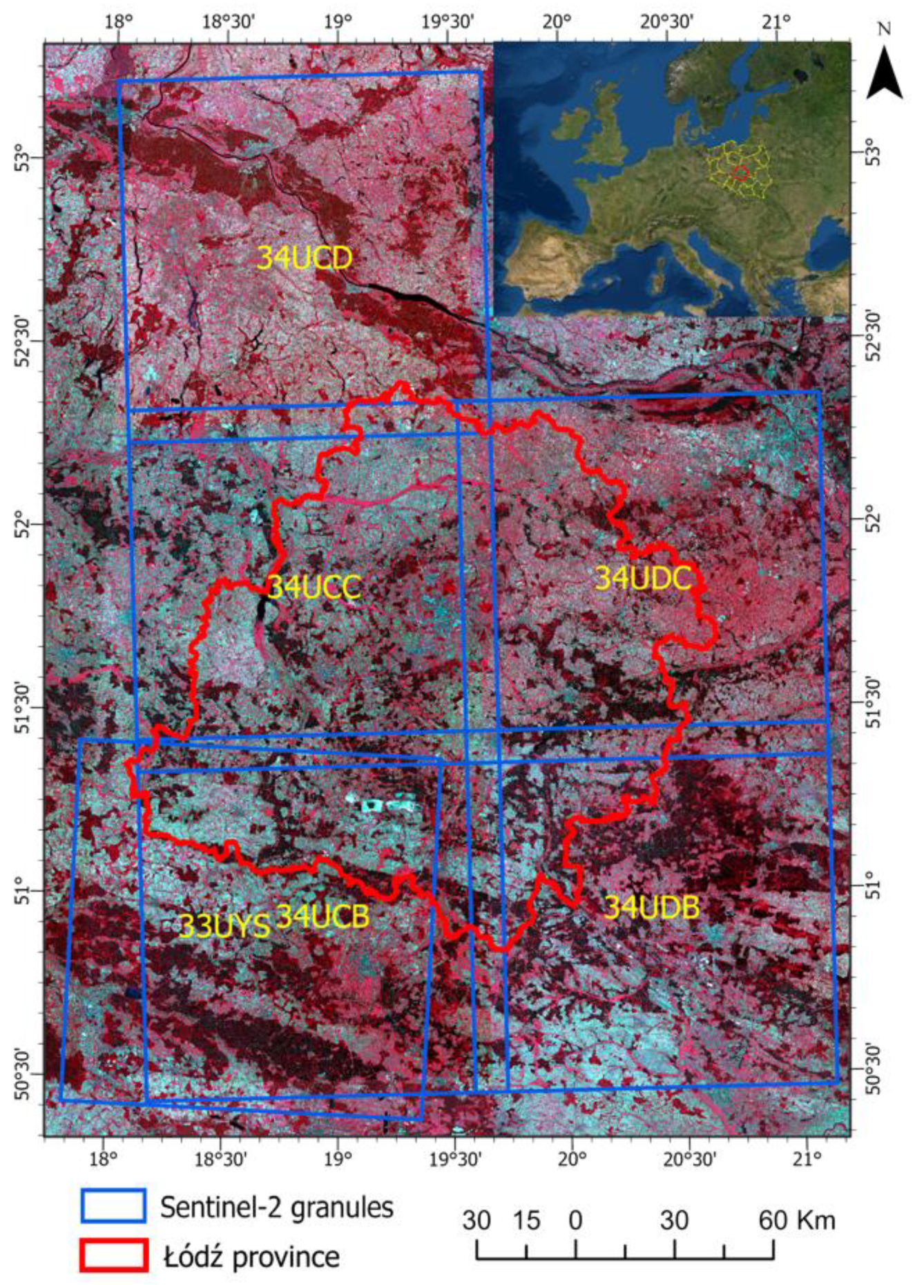
2.1. Study Area

The study area is located in central Poland, with the Łódź province in the middle (Figure 1). The study area covers 57.756 km2 and is delineated by the extent of the six Sentinel-2 granules (100 by 100 km each). It has a lowland character with an average altitude of 169.6 m above sea level. It is covered predominantly by agricultural land with a mosaic of arable land, grasslands, orchards and woody patches. There are a few forest patches located in the South of the study area. There are also large urban areas such as Warsaw (located in the north-east), Łódź or Toruń. The study area represents the typical landscape in Central and Eastern Europe.

2.2. Data

A set of cloud free Sentinel-2A and B images captured between April and September 2020 was downloaded from the ESA Copernicus Data Hub. We used at least four Sentinel-2 scenes representing different phenological seasons for each granule (Table 1). In total, 30 Sentinel-2 images, the Level-2A product, which consist of atmospherically corrected bands with bottom-of-atmosphere calibrated reflectance were processed. The land cover classification was performed for each Sentinel-2 granules individually; therefore, the radiometric adjustment of granules was not performed.
In this study, we used all the Sentinel-2 spectral bands available at 10 m and 20 m spatial resolution; bands at 60 m spatial resolution were not used for the analysis. Bands at 20 m spatial resolution were resampled to 10 m using the bilinear resampling method.

2.3. Reference Dataset
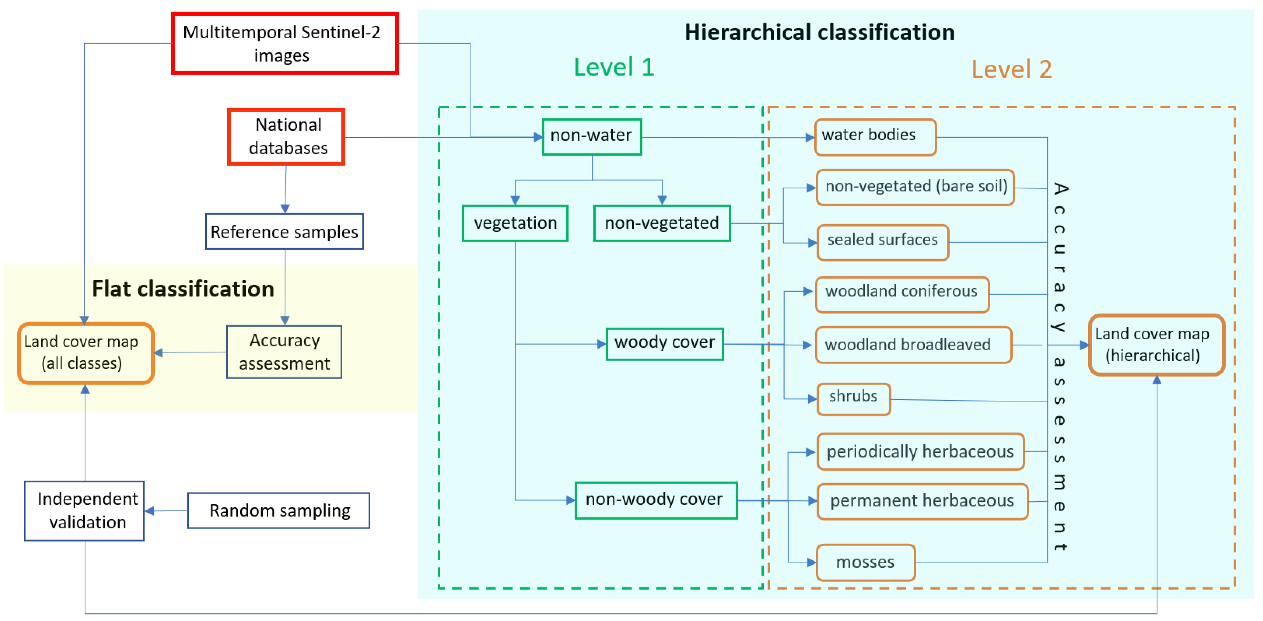
The legend used for land cover mapping corresponds to the CLC+ [53] concept and the Copernicus Global Land Cover [54] (Table 2). The reference data were prepared for all nine land cover classes.
The reference data for land cover classification were derived from the three national databases: the National Topographic Database (BDOT10K), the Forest Data Bank (FDB) and the Land Parcel Identification System (LPIS) managed by the Agency for Restructuring and Modernization of Agriculture (ARiMR). The BDOT10K provides data with a level of detail corresponding to the topographic maps at the 1:10,000 scale. It is a digital, vector database containing the spatial location of topographic objects along with their detailed description. The BDOT10K served as the prime database for selection of the reference sampling plots for the following land cover classes: sealed surfaces, shrubs, mosses, non-vegetated (bare soil), periodically herbaceous and water bodies. To assure the high quality of sampling plots, the periodically herbaceous plots derived from BDOT10K were masked out by the areas assigned as grassland in the ARiMR database. The FDB database served as the source of the reference sampling points for coniferous and broadleaved woodland classes. The forest database provides information on the forest extent, and forest characteristics at the stand level [55]. The forest stands with at least 80% of the broadleaved or deciduous tree species were selected as the reference data for woodland type delineation. The sampling plots for the permanent herbaceous class were extracted from the land cover layer called ‘management fields’, managed by the ARiMR as part of the LPIS. This class was represented by permanent grassland and permanent grassland of natural value classes in LPIS. The LPIS supports the parcel-based subsidies schemes in the EU countries under the Common Agricultural Policy. It provides information at the agricultural parcel level in a vector format. The BDOT10K and ARiMR databases were obtained for the reference year 2018 and FDB for the year 2020. However, it has to be noticed that BDOT10K is derived and updated partially using manual interpretation of aerial orthophotos, thus the reference year for this data within the study area ranged from 2011 to 2018.
In order to minimize the edge effect, the inward buffer of 10 m was applied to the selected reference polygons. For the water bodies class, the 20 m buffer was used to avoid the misclassification of rushes and aquatic vegetation along the shoreline. Next, a set of reference sampling points representing different land cover classes was randomly created in a proportion of 2 points per 1 km2. The exception was the shrubs and mosses classes, representing smaller area, where a minimum of 200 points were created per class. The total number of samples per land cover class for individual Sentinel-2 granule is presented in Table 3. A similar proportion was used for the urban land cover class in Slovakia, Hungary and Poland [45]. The minimum distance between neighbouring sampling points was greater than 20 m.
In the next step, the sampling plots representing woody cover and water classes had to be subject to quality control using the histogram analysis of surface spectral reflectance. This is because of the forest clear cuts according to the national forest definition are classified as forest regardless of the state of forest regrowth. The water bodies in BDOT10K are delimited with the area along the shoreline, thus often the waterlogged areas are included. For sampling points representing these two classes, the average reflectance values for each spectral band were calculated. The threshold values for woody and water classes were determined from the frequency distribution of the spectral reflectance. The threshold values over sampling plots were checked and adjusted manually based on the Sentinel-2 imagery. Consequently, the sampling points located on forest clearings, causeway or rushes were removed. The reference sampling plots were divided using the stratified random sampling method with 60% used for training and 40% validation and for accuracy assessment purposes.

2.4. Methods

2.4.1. Random Forest (RF) Classification

The classification process was performed following two approaches: (1) flat classification, where all nine land cover classes were classified together, and (2) hierarchical classification, where different land cover classes were classified hierarchically. The final land cover hierarchical map was derived as a combination of sub-level results.
We used the RF classifier in Python environment for both classification approaches. The RF classifier is a machine learning technique where many decision trees are constructed based on a random sub-sampling of the given data set [24]. RF includes a set of independent trees to perform the classification task and include random decision tree to classify a dataset by using predictors from a defined number of trees [56].
At first, the standard flat classification was carried out individually on a Sentinel-2 data stack for each single granule. The results were used to develop a scheme of hierarchical classification. To set up the classification hierarchy, we analysed the spectral similarity and class separability, taking into account the error matrix, PA and UA values for each land cover class from the flat classification. The final stratification was set up by experiments. The hierarchical classification was performed in two levels as presented in Figure 2. Level 1 was structured as follows: (i) delineation of water and non-water classes, (ii) the non-water class was classified into vegetation and non-vegetated class, and (iii) the vegetation class was then divided into woody and non-woody cover. Level 2 (more detailed) was structured as follows: (i) the non-vegetated class from Level 1 was separated into non-vegetated bare soil and sealed surfaces, (ii) the woody cover class from Level 1 was separated into woodland coniferous, woodland broadleaved and shrubs, and (iii) the non-woody cover was separated into permanently herbaceous, periodically herbaceous and mosses. The scheme of hierarchical classification was repeated individually over each of the six Sentinel-2 granules covering entire study area. The final hierarchical land cover map was derived as a combination of classification results from Level 1 and 2. The classification scheme for both approaches: hierarchical and flat classification is presented in Figure 2.
Both the flat and hierarchical classifications were carried out using the same input variables (a stack of multi-temporal Sentinel-2 images) and the same set of reference sampling plots. The classification was performed for each granule individuality. The RF models were calibrated using 60% of the reference samples selected using the stratified random sampling. The parameterization of the model was performed on: n_estimators = 100, criterion = ‘entropy’, and random_state = 42.
The final hierarchical land cover map over the entire study area was derived as a combination of classification results from Level 1 and 2. The priority rules used to combine the classification results follow the order of classes presented in Level 2 (Figure 2)—water bodies, non-vegetated subclasses, woody cover subclasses and non-woody cover subclasses. To eliminate single pixels (salt and paper effect), the land cover maps derived using both approaches were filtered using the Nibble filter (window 4 × 4 pixels) available at ArcGIS Pro. The final land cover map for the entire study area was derived by merging the maps determined for individual granules.

2.4.2. Accuracy Assessment

The accuracy assessment of the classification results was carried out for each granule using the validation sampling plots. The classification accuracy was expressed as overall accuracy (OA), F1 score, Kappa coefficient and user’s (UA) and producer’s (PA) accuracy. F1 score is calculated as a weighted average of UA and PA values. For the hierarchical classification, the accuracy assessment was carried out individually for each classification at each level.
Additionally, in order to assess the stability of classification models, we performed both classifications interactively, repeating the classification process 100 times, so a total of 600 classifications were performed for the hierarchical approach and 100 classifications for the flat one. The out-of-bag data error was applied, which is a method of measuring prediction error of random forest classification. This exercise was carried out over one selected representative Sentinel-2 granule (ID 34UCC, Figure 1). The results were presented in the form of box plots. The box plot indicates outliers, first quartile, median, third quartile and maximum values.
Furthermore, to assess the accuracy of the final land cover map derived over the entire study area applying both approaches, we performed independent verification using a random sampling method. In total, 50 verification points per each land cover class was randomly distributed across the study area to assess the quality of land cover classifications [57]. Each verification point was used as centroid to derive the polygons 30 × 30 m. The land cover class was assigned within each of the polygon based on the Sentinel-2 images for the year 2020 with the support of aerial orthophotos. The results of independent land cover accuracy assessment were used to calculate UA, PA values and an error matrix. The same verification approach was used to compare two urban land cover classifications performed by Myint et al. [58].

3. Results

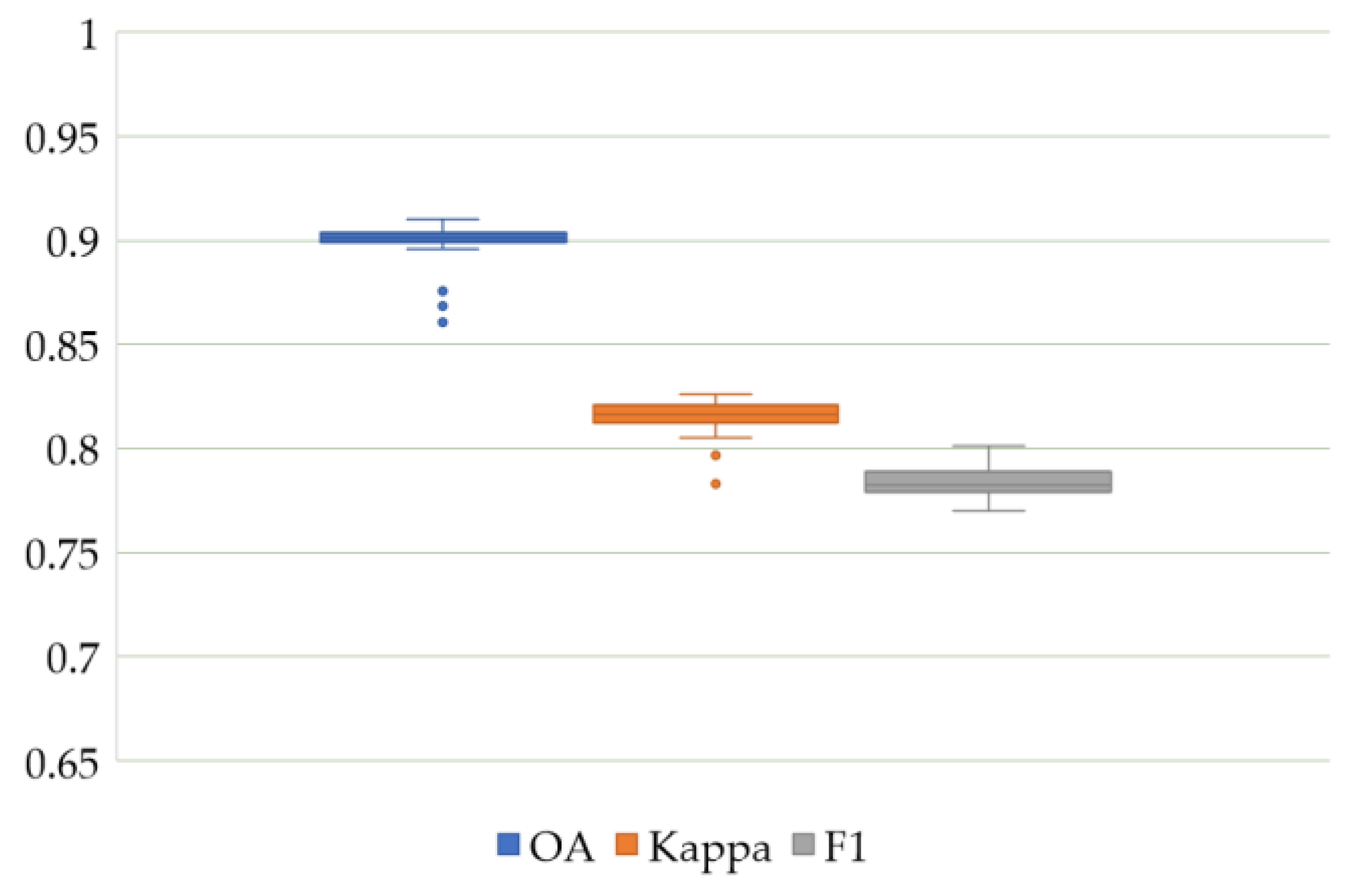
3.1. Flat Classification Accuracy

The flat classification for individual granules reached OA between 0.89 and 0.93, the Kappa coefficient 0.81–0.86, and the F1 score 0.74–0.81. The UA and PA of the individual land cover classes are shown in Table 4.
The highest UA value was achieved for woodland coniferous (0.94 to 0.99) and periodically herbaceous (0.94 to 0.96). The PA for these classes ranged from 0.92 to 0.98 and from 0.90 to 0.94, respectively. The lowest accuracy was obtained for shrubs, mosses and non-vegetated (base soil) classes. Interestingly, the shrubs class was shown to have the most varied accuracy values, which is likely to be related to the spatial distribution of orchards that were classified as shrubs. The large area of orchard is located in the north-eastern part of the study area. The large spread of UA and PA values was also observed for the mosses class, 0.32–0.67 and 0.55–0.79, respectively, as well as for the non-vegetated (bare soil) class, 0.18–0.76 and 0.50–0.89, respectively.
Figure 3 presents the result of the model stability of the flat classification performed for one Sentinel-2 granule.
The median of OA reached the value of 0.90, whereas the Kappa coefficient 0.81 and the F1 score 0.78. The variability of these values is rather low. However, the outliers were observed for OA and Kappa values.

3.2. Hierarchical Classification Accuracy

The accuracy of the hierarchical classification was conducted at Level 1 and 2. The results of the accuracy assessment are presented in Table 5. The OA values for all land cover classes were greater than 0.92. The separation of land cover classes at Level 1 reached an OA of above 0.95, a Kappa coefficient above 0.70 and an F1 larger than 0.85. The lowest F1 score (0.85–0.90) was achieved for the delineation of vegetation/non-vegetated classes, whereas the highest F1 score was above 0.96 for the non-water/water classes.
Slightly low accuracies were achieved for the classification of vegetation/non-vegetated, where the OA reached values of 0.97–0.98, the Kappa 0.70–0.79 and F1 0.85–0.90. The classification of woody/non-woody cover was shown to have the largest spread of OA values, up to four percentage points among six granules.
At Level 2, the highest accuracy was achieved for the classification of coniferous woodland, broadleaved woodland and shrubs carried out within the mask of woody cover from Level 1. The OA of this classification ranged between 0.94and 0.99, Kappa 0.86–0.97 and F1 0.88–0.99. The classification of sealed surfaces/non-vegetated (bare soil) classes within the non-vegetated mask from Level 1 achieved the lowest OA values of 0.92–0.97, Kappa ranging from 0.56 to 0.85 and F1 0.78–0.92. The accuracy of the classification of the non-woody cover class (Level 1) into the permanent herbaceous, periodically herbaceous and mosses classes at Level 2 were comparable to the results of sealed surfaces/non-vegetated (bare soil) classification. However, the spread of values was lower (6–11 percentage points) for non-woody classes compared to sealed surfaces/non-vegetated classes (bare soil) (5–29 percentage points).
Figure 4 presents the variability of the OA, Kappa and F1 values for two levels of hierarchical classification. In Level 1, the OA reached values above 0.97 for three classifications. The highest values of OA, Kappa and F1 score (0.99, 0.98 and 0.98, respectively) were obtained for the classification of non-water/water bodies. This classification model was shown to be the most stable and its classes the most spectrally homogeneous. The classification of vegetation/non-vegetated classes within the mask of the non-water class showed the high values of OA: 0.97, Kappa: 0.75 and F1: 0.87. Similarly, the OA value (0.94) was achieved in the classification of woody/non-woody classes within the mask of vegetated class. Here, the Kappa and F1 reached values of 0.92 and 0.96, respectively. Slightly lower accuracy was achieved for the classifications at Level 2.
The classification of coniferous and broadleaved woodland and shrubs, within the mask of woody class from Level 1, showed to be the most stable and the most accurate compared to other classes. The classification accuracy for these classes achieved values of OA 0.96, Kappa 0.90 and F1 0.92. Slightly worst results were obtained for the classification of permanent herbaceous, periodically herbaceous and mosses classes, reaching the OA of 0.95, Kappa of 0.78 and F1 of 0.86. These classes, due to the spectral characteristics, agriculture activities and phenology cycle, are difficult to delineate accurately. However, the classification models were shown to be quite stable. The largest variability of accuracy was observed for the classification of sealed surfaces/non-vegetated (bare soil) classes, where the Kappa values ranged from 0.70 to 0.85 and the F1 values from 0.85 to 0.92.
The final land cover map over the entire study area as the result of the hierarchical classification is presented in Figure 5.

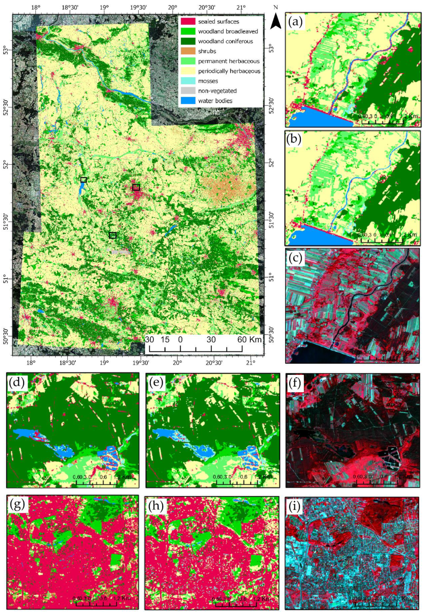
3.3. Independent Verification of the Results of the Flat and Hierarchical Classification

The results of the independent verification of the land cover maps over the entire study area derived using flat and hierarchical approaches are presented in Table 6.
The results confirmed that the hierarchical approach provided more accurate land cover maps compared to the flat classification. The UA of hierarchical classification was higher for all the land cover classes compared to the flat classification, except the sealed surface and woodland broadleaved classes, where the values were slightly lower. The highest UA was achieved for the following classes: mosses (1.00), water (0.96), non-vegetated (0.92), and woodland coniferous (0.91). For the water bodies class, the UA was equal to 0.96 for both classifications. The highest difference in UA values between the hierarchical and flat classifications was obtained for mosses (18 percentage points), permanent herbaceous (18 percentage points) and woodland coniferous (15 percentage points) classes.
Interestingly, the lowest UA values below 0.8 were obtained in both classifications for shrubs, sealed surfaces and woody broadleaved classes. The shrubs were partially misclassified as broadleaved woodland, mosses and permanent herbaceous. By contrast, the broadleaved woodlands were mixed up with shrubs. Sometimes the periodically herbaceous areas were misclassified as permanently herbaceous. Furthermore, the sealed surfaces were mixed up with the bare soil and vice versa. Around 20% of non-vegetated (bare soil) sampling polygons were misclassified as sealed surfaces.
The PA values of hierarchical classification were higher for six land cover classes compared to the flat approach. The PA of the flat classification reached higher values for two classes: permanent herbaceous (8 percentage points) and periodically herbaceous (10 percentage points) compared to the hierarchical classification. The largest differences in PA for both classifications were observed for sealed surfaces (18 percentage points), woodland broadleaved (14 percentage points) and woodland coniferous (12 percentage points). The lowest PA values for the flat classification were achieved for mosses (0.64), non-vegetated (0.66) and shrubs (0.70) classes. For comparison, in the hierarchical approach, the lowest PA was achieved for non-vegetated (0.68), periodically herbaceous (0.70) and mosses (0.74) classes. For the water bodies class, the PA was the same (0.98) in both classifications. The lowest PA values in both classifications (below 0.8) were achieved for shrubs, periodically herbaceous, mosses and non-vegetated (bare soil) classes.
Additionally, to assess the quality of the final land cover maps, we performed the visual comparison of the classification results versus the Sentinel-2 data and aerial orthophotos. Figure 5 presents the final hierarchical land cover map for the entire study area and a few examples of more detailed results of both classifications. There is a quite good agreement with the reference data observed for the hierarchical classification. There is a visible misclassification of areas along the river or water bodies, which were assigned as sealed surfaces in the flat classification (Figure 5a). By contrast, in the hierarchical classification, these areas are assigned as water or mosses, which is the real land cover type (Figure 5b). The example in Figure 5a,c presents the large overestimation of sealed surfaces along the edges of ponds and forest clearcuts, especially on the forest edges. These areas are correctly classified as woodlands, water or mosses in the hierarchical approach (Figure 5b,d). The flat approach also underestimated the mosses areas, which were classified partially as water bodies. The densely built-up areas with high buildings were better classified in the flat approach (Figure 5e,f), because of shadows of high buildings were misclassified as mosses in the hierarchical classification. On the other hands, the flat approach did not pick up the urban greenery structure very well (Figure 5e) and in general is less detailed compared to the hierarchical one.

4. Discussion

In this study, we examined whether the land cover classification carried out using the hierarchical approach can provide more accurate and reliable results than the standard flat method. It has to be stressed that the number of studies on hierarchical classification of land cover types is rather limited. There are only a few studies conducting the pixel-based hierarchical classification using multispectral satellite images. Most of other studies focus on the examination of hierarchical approach towards the object-based (OBIA) classification of hyperspectral data or fusion of multispectral and hyperspectral data. Compared to the results of other studies for the land cover mapping using hierarchical and flat methods, our results are comparable or more accurate. We proved that the stratified, hierarchical approach to land cover classification gave more accurate results compared to the standard flat method. The OA and F1 increased on average by 5 and 12 percentage points, respectively, by applying the hierarchical classification. The differences in accuracy between two approaches was more pronounced in complex classes such as mosses, shrubs, sealed surfaces and non-vegetated. The hierarchical approach increased the separability of complex classes. Jiao et al. [59] examined the hierarchical approach for mapping coastal wetlands in China using the Landsat data and obtained more accurate results to ours. The authors achieved the OA values of 0.93–0.96, UA around 0.99 and PA 0.97. Much lower UA and PA values for mosses class were achieved in our study, in the flat classification UA and PA ranged from 0.32 to 0.73 and 0.55 to 0.79, respectively, whereas in the hierarchical the UA and PA for this class reached values of 1.00 and 0.74, respectively. The differences in the obtained results can be related to the fact that Jiao et al. [59] in the first level adopted the expert rules of spectral variables based on spectra indices and then in the second level utilised the machine learning approach (SVM classifier). In addition, the study was rather local.
Myint et al. [58] compared a pixel-based flat classification and object-based hierarchical classification of urban land cover in the city of Phoenix (USA) based on very high resolution QuickBird images. The authors used the nearest neighbour classifier. They confirmed the advantage of the hierarchical classification over the standard flat classification. The OA of the flat classification result reached a value of 0.63, whereas in the hierarchical approach the OA varied between 0.80 and 0.99. This is in line with the results for land cover mapping obtained in our study. The overall accuracy of the hierarchical classification of land cover carried out by Demirkan et al. [49] in Turkey using Sentinel-2 data and RF method is lower than that obtained in our study. The authors performed classification at two levels: first, general classes, and second more detailed land cover classes. They achieved the OA of 0.84–0.85 for Level 1 and 0.72–0.82 for Level 2. To compare, in our study, values of OA were much higher and reached 0.97–0.99 in Level 1 and 0.92–0.97 in Level 2. The difference may be caused by using the NDVI and NDWI spectral indices and applying the threshold in Level 1 instead of the classification. In addition, they used a single image instead of the time series of Sentinel-2 used in our study.
Interestingly, Clark [42] stressed out the importance of the references sampling strategy in the classification process. They applied the RF method to classify twelve land cover classes using Sentinel-2 data in the San Francisco Bay area. The authors achieved a higher OA of 0.84 for the reference sampling polygons compared to 0.80 of OA for the reference sampling point strategy. In our study, we applied the reference sampling points and obtained higher OA for land cover classification.
Our results confirmed that classes such as mosses, shrubs and non-vegetated bare soil are the most difficult to delineate and separate using the flat standard approach. These classes showed also the higher level of variability. The independent verification of the land cover maps performed over the entire study area confirmed the superiority of the hierarchical approach. The lowest PA values in both classifications (below 0.8) were achieved for shrubs, periodically herbaceous, mosses and non-vegetated classes. Around 20% of non-vegetated sampling polygons were misclassified as sealed surfaces. In addition, the shrubs class were shown to have the highest variability of the accuracy values, which is probably related to the spatial pattern of orchards that were classified as shrubs. The orchards are characterised by heterogenous structure and mixed pixels, which affects the accurate delineation of this class. In the flat classification, the lowest PA values were achieved for mosses (0.64), non-vegetated (0.66) and shrubs (0.70) classes. To compare, in the hierarchical approach the lowest PA was achieved for non-vegetated (0.68), periodically herbaceous (0.70) and mosses (0.74) classes. The mosses/wetland class was pointed out by Ghorbanian et al. [41] as the most challenging class for delineation using Sentinel-2 imagery. Over the 13 land cover classes, the wetlands reached the lowest PA and UA values of 0.89 and 0.86, respectively. Difficulties in delineation of wetland classes were also reported by Whyte et al. [42] in South Africa. The authors classified 15 land cover classes using RF classifier and Sentinel-2 data and achieved the lowest values of UA and PA of 0.60 and 0.66 for three wetland classes, respectively. Interestingly, they also reported the lowest UA and PA for bare soil (0.62–0.68) and shrubs (0.65–0.73) classes. These three classes were also recognised as the most challenging to classify by our study. The sealed surfaces were sometimes mixed up with the bare soil and vice versa. This may be related to the spectral similarity of some roofs and bare ground, mixed pixels and the difficulty of detecting narrow roads or smaller buildings. The analysis of the model stability also confirmed that the classification of sealed surfaces/non-vegetated classes is less stable, showing high variability.
The highest increase in the PA of the hierarchical approach compared to the flat one was observed for sealed surfaces, broadleaved woodland, coniferous woodland and mosses, by 18, 14, 12 and 10 percentage points, respectively. It confirms the superiority of hierarchical classification over flat classification. For two herbaceous classes, the PA was higher in the flat classification, by 10 and 8 percentage points for periodically and permanent herbaceous, respectively. The independent verification showed that the periodically herbaceous areas were sometimes misclassified as permanently herbaceous. This was also observed by Bobáľová et al. [45]. The authors tested the hierarchical OBIA approach for classification of six land cover classes in selected cities in Central Europe using Sentinel-2 data and concluded that the most problematic classes are dry grass and cropland classes. They achieved the lowest UA of 0.40–0.86 for dry grass and 0.32–0.93 for cropland classes, and the highest OA value above 0.90 for the forest class.
As part of this study, we analysed the advantages and disadvantages of both classification approaches. The main advantages of the flat classification are (i) the simplicity of the classification process, because all classes are classified together, and (ii) very short execution time. The main disadvantage is related to the lower accuracy of individual classes; less representative classes are especially underestimated. In comparison, the main advantages of the hierarchical classification are (i) more accurate and reliable results, and (ii) developing additional intermediate products as the outputs of the hierarchical stratification of land cover classes. The High-Resolution Layers for 2018 (HRL) provided by the Copernicus Land Monitoring Service (CLMS) are the examples of the individual land cover classes derived from the automatic classification of Sentinel-2 and Sentinel-1 images. There are four HRL2018 products: imperviousness, forest, grasslands, water and wetness available at CLMS [60]. In general, the HRLs correspond to the group of land cover classes in hierarchical classification. The biggest disadvantage of hierarchical classification is the complexity of the classification process. It requires performance of several classifications instead of one. In this study, we performed six classifications, which prolongs the processing time. In addition, the process of stratification of land cover classes is based on many experiments. There is no universal rule how to divide land cover classes in the hierarchy structure. In our study, the process of classification, likely in other studies, was preceded by testing different features and parameters using the trial-and-error method [45]. Jiao et al. [59], mapping wetlands in China, have come to similar conclusions that it is hard to define one universe class hierarchy for different study areas.
The analysis of the stability of the RF classification models performed in this study confirmed that the hierarchical approach provides, on one hand, more accurate results but on the other is characterised by the greater variability of accuracy values than the flat classification. In the hierarchical approach, the most stable results were achieved for the non-water/water and woody/non-woody cover classification in Level 1 and the classification of woodland coniferous, broadleaved and shrubs in Level 2. The values of OA, Kappa and F1 for these classifications varied by 2–4 percentage points. The least stable and the lowest classifications accuracy was obtained for the vegetation/non-vegetated cover in Level 1 and for sealed surfaces/non-vegetated (bare soil) classification in Level 2. The Kappa coefficient for these two classifications varied from 0.72 to 0.78 in Level 1 and from 0.70 to 0.85 in Level 2. It was related to the problem in misclassifying shadows of the high buildings as the mosses class. Myint et al. [58] also found that shadows around high buildings may cause misclassification on urban areas. In flat classification, the model was more stable but gave lower classification accuracy. The results of our study showed that some of the classes such as woody cover and water bodies are easy to separate with high accuracy using both approaches and some are more difficult such as non-vegetated (base soil), mosses and shrubs. The most complex classes were also recognised as problematic to delineate in other studies [43,44].

5. Conclusions

The hierarchical classification approach produced more accurate and reliable land cover classification results than the standard flat method. The overall accuracy of the land cover classification increased by three to seven percentage points by applying the hierarchical approach. The hierarchical approach gave higher user’s accuracy for five out of nine land cover classes, one class was on the same level and for three it fell slightly compared to the flat classification. The producer’s accuracy was also higher for six out of nine classes, one was on the same level and two decreased be a few percentage points. In addition, the hierarchical approach gave better visual results, which are closer to reality than the flat classification. The great advantage of the hierarchical approach is the production of the additional products that can be used for various purposes. However, it has to be highlighted that the biggest disadvantage of the hierarchic approach is the complexity of the classification process, which makes it time-consuming.

Author Contributions

Conceptualization, A.W. and A.H.; Methodology, A.W. and A.H.; Validation, A.W. and M.C.; Formal analysis, A.W.; Investigation, A.W.; Data curation, A.W.; Writing—original draft, A.W.; Writing—review & editing, A.H. and M.C.; Visualization, A.W.; Supervision, A.H.; Funding acquisition, A.H.; Project administration, A.H. All authors have read and agreed to the published version of the manuscript.

Funding

The research leading to these results has received funding from the Norway Grants 2014–2021 via the National Center for Research and Development [grant no: NOR/POLNOR/InCoNaDa/0050/2019-00].

Institutional Review Board Statement

Not applicable.

Informed Consent Statement

Not applicable.

Data Availability Statement

Not applicable.

Conflicts of Interest

The authors declare no conflict of interest.

References

  1. Mohanrajan, S.N.; Loganathan, A.; Manoharan, P. Survey on Land Use/Land Cover (LU/LC) change analysis in remote sensing and GIS environment: Techniques and Challenges. Environ. Sci. Pollut. Res. 2020, 27, 29900–29926. [Google Scholar] [CrossRef] [PubMed]
  2. Mazzia, V.; Khaliq, A.; Chiaberge, M. Improvement in Land Cover and Crop Classification based on Temporal Features Learning from Sentinel-2 Data Using Recurrent-Convolutional Neural Network (R-CNN). Appl. Sci. 2020, 10, 238. [Google Scholar] [CrossRef] [Green Version]
  3. Borges, J.; Higginbottom, T.P.; Symeonakis, E.; Jones, M. Sentinel-1 and Sentinel-2 Data for Savannah Land Cover Mapping: Optimising the Combination of Sensors and Seasons. Remote Sens. 2020, 12, 3862. [Google Scholar] [CrossRef]
  4. Brovelli, M.A.; Sun, Y.; Yordanov, V. Monitoring Forest Change in the Amazon Using Multi-Temporal Remote Sensing Data and Machine Learning Classification on Google Earth Engine. ISPRS Int. J. Geo-Inf. 2020, 9, 580. [Google Scholar] [CrossRef]
  5. Häme, T.; Sirro, L.; Kilpi, J.; Seitsonen, L.; Andersson, K.; Melkas, T. A Hierarchical Clustering Method for Land Cover Change Detection and Identification. Remote Sens. 2020, 12, 1751. [Google Scholar] [CrossRef]
  6. Topaloglu, H.R.; Sertel, E.; Musaoglu, N. Assessment of classification accuracies of SENTINEL-2 and LANDSAT-8 data for land cover/use mapping. Int. Arch. Photogramm. Remote Sens. Spat. Inf. Sci. 2016, 41, 1055–1059. [Google Scholar] [CrossRef] [Green Version]
  7. Rujoiu-Mare, M.-R.; Olariu, B.; Mihai, B.-A.; Nistor, C.; Săvulescu, I. Land cover classification in Romanian Carpathians and Subcarpathians using multi-date Sentinel-2 remote sensing imagery. Eur. J. Remote Sens. 2017, 50, 496–508. [Google Scholar] [CrossRef] [Green Version]
  8. Jucker, T.; Caspersen, J.; Chave, J.; Antin, C.; Barbier, N.; Bongers, F.; Dalponte, M.; Van Ewijk, K.Y.; Forrester, D.I.; Haeni, M.; et al. Allometric equations for integrating remote sensing imagery into forest monitoring programmes. Glob. Chang. Biol. 2017, 23, 177–190. [Google Scholar] [CrossRef] [Green Version]
  9. Khatami, R.; Mountrakis, G.; Stehman, S.V. A meta-analysis of remote sensing research on supervised pixel-based land-cover image classification processes: General guidelines for practitioners and future research. Remote Sens. Environ. 2016, 177, 89–100. [Google Scholar] [CrossRef] [Green Version]
  10. Randazzo, G.; Cascio, M.; Fontana, M.; Gregorio, F.; Lanza, S.; Muzirafuti, A. Mapping of Sicilian Pocket Beaches Land Use/Land Cover with Sentinel-2 Imagery: A Case Study of Messina Province. Land 2021, 10, 678. [Google Scholar] [CrossRef]
  11. Ye, J.; Hu, Y.; Zhen, L.; Wang, H.; Zhang, Y. Analysis on Land-Use Change and Its Driving Mechanism in Xilingol, China, during 2000–2020 Using the Google Earth Engine. Remote Sens. 2021, 13, 5134. [Google Scholar] [CrossRef]
  12. Campbell, J.B.; Wynne, R.H. Introduction to Remote Sensing; Guilford Press: New York, NY, USA, 2011; Volume 5. [Google Scholar]
  13. Phiri, D.; Morgenroth, J. Developments in Landsat Land Cover Classification Methods: A Review. Remote Sens. 2017, 9, 967. [Google Scholar] [CrossRef] [Green Version]
  14. Da Ponte, E.; Mack, B.; Wohlfart, C.; Rodas, O.; Fleckenstein, M.; Oppelt, N.; Dech, S.; Kuenzer, C. Assessing Forest Cover Dynamics and Forest Perception in the Atlantic Forest of Paraguay, Combining Remote Sensing and Household Level Data. Forests 2017, 8, 389. [Google Scholar] [CrossRef] [Green Version]
  15. Waśniewski, A.; Hościło, A.; Zagajewski, B.; Moukétou-Tarazewicz, D. Assessment of Sentinel-2 Satellite Images and Random Forest Classifier for Rainforest Mapping in Gabon. Forests 2020, 11, 941. [Google Scholar] [CrossRef]
  16. Hościło, A.; Lewandowska, A. Mapping Forest Type and Tree Species on a Regional Scale Using Multi-Temporal Sentinel-2 Data. Remote Sens. 2019, 11, 929. [Google Scholar] [CrossRef] [Green Version]
  17. Fagan, M.; Defries, R.; Sesnie, S.; Arroyo-Mora, J.; Soto, C.; Singh, A.; Townsend, P.; Chazdon, R. Mapping Species Composition of Forests and Tree Plantations in Northeastern Costa Rica with an Integration of Hyperspectral and Multitemporal Landsat Imagery. Remote Sens. 2015, 7, 5660–5696. [Google Scholar] [CrossRef] [Green Version]
  18. Robertson, L.D.; King, D. Comparison of pixel- and object-based classification in land cover change mapping. Int. J. Remote Sens. 2013, 32, 1505–1529. [Google Scholar] [CrossRef]
  19. ESA. Sentinel-2 Missions-Sentinel Online; ESA: Paris, France. Available online: https://sentinel.esa.int/web/sentinel/missions/sentinel-2 (accessed on 9 January 2022).
  20. Drusch, M.; Del Bello, U.; Carlier, S.; Colin, O.; Fernandez, V.; Gascon, F.; Hoersch, B.; Isola, C.; Laberinti, P.; Martimort, P.; et al. Sentinel-2: ESA’s Optical High-Resolution Mission for GMES Operational Services. Remote Sens. Environ. 2012, 120, 25–36. [Google Scholar] [CrossRef]
  21. Forkuor, G.; Dimobe, K.; Serme, I.; Tondoh, J.E. Landsat-8 vs. Sentinel-2: Examining the added value of sentinel-2’s red-edge bands to land-use and land-cover mapping in Burkina Faso. GIScience Remote Sens. 2018, 55, 331–354. [Google Scholar] [CrossRef]
  22. Delegido, J.; Verrelst, J.; Alonso, L.; Moreno, J. Evaluation of Sentinel-2 Red-Edge Bands for Empirical Estimation of Green LAI and Chlorophyll Content. Sensors 2011, 11, 7063–7081. [Google Scholar] [CrossRef] [Green Version]
  23. Kussul, N.; Lavreniuk, M.; Skakun, S.; Shelestov, A. Deep learning classification of land cover and crop types using remote sensing data. IEEE Geosci. Remote Sens. Lett. 2017, 14, 778–782. [Google Scholar] [CrossRef]
  24. Phiri, D.; Simwanda, M.; Salekin, S.; Nyirenda, V.; Murayama, Y.; Ranagalage, M. Sentinel-2 Data for Land Cover/Use Mapping: A Review. Remote Sens. 2020, 12, 2291. [Google Scholar] [CrossRef]
  25. Zanaga, D.; Van De Kerchove, R.; De Keersmaecker, W.; Souverijns, N.; Brockmann, C.; Quast, R.; Wevers, J.; Grosu, A.; Paccini, A.; Vergnaud, S.; et al. ESA WorldCover 10 m 2020 v100; European Space Agency: Brussels, Belgium, 2021. [Google Scholar]
  26. Karra, K.; Kontgis, C.; Statman-Weil, Z.; Mazzariello, J.C.; Mathis, M.; Brumby, S.P. Global land use/land cover with Sentinel 2 and deep learning. In Proceedings of the 2021 IEEE International Geoscience and Remote Sensing Symposium IGARSS, Brussels, Belgium, 11–16 July 2021; pp. 4704–4707. [Google Scholar] [CrossRef]
  27. Malinowski, R.; Lewiński, S.; Rybicki, M.; Gromny, E.; Jenerowicz, M.; Krupiński, M.; Nowakowski, A.; Wojtkowski, C.; Krupiński, M.; Krätzschmar, E.; et al. Automated Production of a Land Cover/Use Map of Europe Based on Sentinel-2 Imagery. Remote Sens. 2020, 12, 3523. [Google Scholar] [CrossRef]
  28. Olsen, J.B. Technical Specifications for Implementation of a New Land-Monitoring Concept Based on EAGLE. Public Consultation Document for CLC+ Core; European Environment Agency: Copenhagen, Denmark, 2020. [Google Scholar]
  29. Europe’s Eyes on Earth; Land Monitoring Service. CLC+. Available online: https://land.copernicus.eu/pan-european/clc-plus (accessed on 7 November 2021).
  30. Steinhausen, M.J.; Wagner, P.D.; Narasimhan, B.; Waske, B. Combining Sentinel-1 and Sentinel-2 data for improved land use and land cover mapping of monsoon regions. Int. J. Appl. Earth Obs. Geoinf. 2018, 73, 595–604. [Google Scholar] [CrossRef]
  31. Cortes, C.; Vapnik, V. Support-vector networks. Mach. Learn. 1995, 20, 273–297. [Google Scholar] [CrossRef]
  32. Aghdam, H.H.; Heravi, E.J. Guide to Convolutional Neural Networks: A Practical Application to Traffic-Sign Detection and Classification; Springer Publishing Company, Incorporated: Berlin/Heidelberg, Germany, 2017. [Google Scholar]
  33. Jamali, A. Evaluation and comparison of eight machine learning models in land use/land cover mapping using Landsat 8 OLI: A case study of the northern region of Iran. SN Appl. Sci. 2019, 1, 1448. [Google Scholar] [CrossRef] [Green Version]
  34. Thanh Noi, P.; Kappas, M. Comparison of Random Forest, k-Nearest Neighbor, and Support Vector Machine Classifiers for Land Cover Classification Using Sentinel-2 Imagery. Sensors 2017, 18, 18. [Google Scholar] [CrossRef] [Green Version]
  35. Amani, M.; Brisco, B.; Afshar, M.; Mirmazloumi, S.M.; Mahdavi, S.; Mirzadeh, S.M.J.; Huang, W.; Granger, J. A generalized supervised classification scheme to produce provincial wetland inventory maps: An application of Google Earth Engine for big geo data processing. Big Earth Data 2019, 3, 378–394. [Google Scholar] [CrossRef]
  36. Dabija, A.; Kluczek, M.; Zagajewski, B.; Raczko, E.; Kycko, M.; Al-Sulttani, A.H.; Tardà, A.; Pineda, L.; Corbera, J. Comparison of Support Vector Machines and Random Forests for Corine Land Cover Mapping. Remote Sens. 2021, 13, 777. [Google Scholar] [CrossRef]
  37. Inglada, J.; Arias, M.; Tardy, B.; Hagolle, O.; Valero, S.; Morin, D.; Dedieu, G.; Sepulcre, G.; Bontemps, S.; Defourny, P.; et al. Assessment of an Operational System for Crop Type Map Production Using High Temporal and Spatial Resolution Satellite Optical Imagery. Remote Sens. 2015, 7, 12356–12379. [Google Scholar] [CrossRef] [Green Version]
  38. Adam, E.; Mutanga, O.; Odindi, J.; Abdel-Rahman, E.M. Land-use/cover classification in a heterogeneous coastal landscape using RapidEye imagery: Evaluating the performance of random forest and support vector machines classifiers. Int. J. Remote Sens. 2014, 35, 3440–3458. [Google Scholar] [CrossRef]
  39. Nguyen, H.T.T.; Doan, T.M.; Tomppo, E.; McRoberts, R.E. Land Use/Land Cover Mapping Using Multitemporal Sentinel-2 Imagery and Four Classification Methods—A Case Study from Dak Nong, Vietnam. Remote Sens. 2020, 12, 1367. [Google Scholar] [CrossRef]
  40. Woznicki, S.A.; Baynes, J.; Panlasigui, S.; Mehaffey, M.; Neale, A. Development of a spatially complete floodplain map of the conterminous United States using random forest. Sci. Total Environ. 2019, 647, 942–953. [Google Scholar] [CrossRef]
  41. Rodriguez-Galiano, V.F.; Ghimire, B.; Rogan, J.; Chica-Olmo, M.; Rigol-Sanchez, J.P. An assessment of the effectiveness of a random forest classifier for land-cover classification. ISPRS J. Photogramm. Remote Sens. 2012, 67, 93–104. [Google Scholar] [CrossRef]
  42. Clark, M.L. Comparison of simulated hyperspectral HyspIRI and multispectral Landsat 8 and Sentinel-2 imagery for multi-seasonal, regional land-cover mapping. Remote Sens. Environ. 2017, 200, 311–325. [Google Scholar] [CrossRef]
  43. Ghorbanian, A.; Kakooei, M.; Amani, M.; Mahdavi, S.; Mohammadzadeh, A.; Hasanlou, M. Improved land cover map of Iran using Sentinel imagery within Google Earth Engine and a novel automatic workflow for land cover classification using migrated training samples. ISPRS J. Photogramm. Remote Sens. 2020, 167, 276–288. [Google Scholar] [CrossRef]
  44. Whyte, A.; Ferentinos, K.P.; Petropoulos, G.P. A new synergistic approach for monitoring wetlands using Sentinels -1 and 2 data with object-based machine learning algorithms. Environ. Model. Softw. 2018, 104, 40–54. [Google Scholar] [CrossRef] [Green Version]
  45. Bobáľová, H.; Benová, A.; Kožuch, M. Hierarchical Object-Based Mapping of Urban Land Cover Using Sentinel-2 Data: A Case Study of Six Cities in Central Europe. PFG–J. Photogramm. Remote Sens. Geoinf. Sci. 2021, 89, 15–31. [Google Scholar] [CrossRef]
  46. Rahdari, V.; Soffianian, A.; Pourmanafi, S.; Mosadeghi, R.; Mohammadi, G.H. A hierarchical approach of hybrid image classification for land use and land cover mapping. Geogr. Pannonica 2018, 22, 30–39. [Google Scholar] [CrossRef] [Green Version]
  47. Sánchez, J.; Perronnin, F.; Mensink, T.; Verbeek, J. Image Classification with the Fisher Vector: Theory and Practice. Int. J. Comput. Vis. 2013, 105, 222–245. [Google Scholar] [CrossRef]
  48. Avci, M. A Hierarchical classification of Landsat TM Imagery For Landcover Mapping. Int. Soc. Photogramm. Remote Sens. 2004, IV. [Google Scholar]
  49. Demirkan, D.; Koz, A.; Düzgün, H. Hierarchical classification of Sentinel 2-a images for land use and land cover mapping and its use for the Corine system. J. App. Remote Sens. 2020, 14, 026524. [Google Scholar] [CrossRef]
  50. Peña, J.; Gutiérrez, P.; Hervás-Martínez, C.; Six, J.; Plant, R.; López-Granados, F. Object-Based Image Classification of Summer Crops with Machine Learning Methods. Remote Sens. 2014, 6, 5019–5041. [Google Scholar] [CrossRef] [Green Version]
  51. Haest, B.; Vanden Borre, J.; Spanhove, T.; Thoonen, G.; Delalieux, S.; Kooistra, L.; Mücher, C.; Paelinckx, D.; Scheunders, P.; Kempeneers, P. Habitat Mapping and Quality Assessment of NATURA 2000 Heathland Using Airborne Imaging Spectroscopy. Remote Sens. 2017, 9, 266. [Google Scholar] [CrossRef] [Green Version]
  52. Freeman, E.A.; Moisen, G.G.; Coulston, J.W.; Wilson, B.T. Random forests and stochastic gradient boosting for predicting tree canopy cover: Comparing tuning processes and model performance. Can. J. For. Res. 2016, 46, 323–339. [Google Scholar] [CrossRef] [Green Version]
  53. Kleeschulte, S.; Banko, G.; Smith, G.; Arnold, S.; Scholz, J.; Kosztra, B.; Maucha, G. Maucha Technical Specifications for Implementation of a New Land-Monitoring Concept Based on EAGLE. D3: Draft Design Concept and CLC-Backbone, CLC-Core Technical Specifications, Including Requirements Review; European Environment Agency: Copenhagen, Denmark, 2017; p. 79. [Google Scholar]
  54. Zanaga, D.; Van De Kerchove, R.; De Keersmaecker, W.; Lesiv, M.; Li, L.; Tsendbazar, N.E. ESA WorldCover 10 m 2020 v1. Product User Manual; European Space Agency: Brussels, Belgium, 2020. [Google Scholar]
  55. BDL. Bank Danych o Lasach. Available online: https://www.bdl.lasy.gov.pl/portal/opis-bdl (accessed on 3 September 2021).
  56. Breiman, L. Random Forests. Mach. Learn. 2001, 45, 5–32. [Google Scholar] [CrossRef] [Green Version]
  57. Congalton, R.G. A review of assessing the accuracy of classifications of remotely sensed data. Remote Sens. Environ. 1991, 37, 35–46. [Google Scholar] [CrossRef]
  58. Myint, S.W.; Gober, P.; Brazel, A.; Grossman-Clarke, S.; Weng, Q. Per-pixel vs. object-based classification of urban land cover extraction using high spatial resolution imagery. Remote Sens. Environ. 2011, 115, 1145–1161. [Google Scholar] [CrossRef]
  59. Jiao, L.; Sun, W.; Yang, G.; Ren, G.; Liu, Y. A Hierarchical Classification Framework of Satellite Multispectral/Hyperspectral Images for Mapping Coastal Wetlands. Remote Sens. 2019, 11, 2238. [Google Scholar] [CrossRef] [Green Version]
  60. Europe’s Eyes on Earth. High Resolution Layers. Available online: https://land.copernicus.eu/pan-european/high-resolution-layers (accessed on 13 December 2021).
Figure 1. Location of the study site. Blue polygons indicate the extant of six Sentinel-2 granules (the colour composite: bands 8, 3 and 2) with the red outline of the Łódź province.
Remotesensing 14 00989 g001
Figure 2. Flowchart of the flat and hierarchical classification of land cover using Sentinel-2 data.
Remotesensing 14 00989 g002
Figure 3. Variability of overall accuracy (OA), Kappa coefficient and F1 score for the flat classification—result of 100 iterations run over the 34UCC granule. The box plot indicates outliers, first quartile, median, third quartile and maximum values.
Remotesensing 14 00989 g003
Figure 4. Variability of overall accuracy (OA), Kappa coefficient and F1 scores for the hierarchical classification at Level 1 and 2—the results of 100 classification iterations performed on the Sentinel-2 granule no. 34UCC.
Remotesensing 14 00989 g004
Figure 5. The land cover map of the entire study area derived based on hierarchical classification. Black squares indicate the location of the areas presented on a larger scale as the result of the flat classification (a,d,g), hierarchical classification (b,e,h) and S-2 colour composite: bands 843 (c,f,i).
Remotesensing 14 00989 g005
Table 1. A set of Sentinel-2 data used in the classification process.
Granule ID33UYS34UCB34UCC34UCD34UDB34UDC
Acquisition data2020-04-122020-04-122020-04-122020-04-052020-04-092020-04-07
2020-07-012020-07-012020-06-012020-05-152020-05-092020-05-09
2020-07-312020-07-312020-07-012020-06-012020-07-012020-06-01
2020-09-142020-09-092020-08-052020-08-052020-08-122020-07-01
2020-09-142020-08-202020-09-142020-08-12
2020-09-22 2020-09-14
Table 2. Land cover class nomenclature; definitions correspond to the Copernicus Global Land Cover.
Land Cover ClassDefinition
Sealed surfacesLand covered by buildings, roads and other human-made structures such as railroads. Buildings include both residential and industrial built-up areas.
Woodland broadleavedLand cover dominated by trees with cover of 10% or more; 80% or more tree species should be broadleaved.
Woodland coniferousLand cover dominated by trees with cover of 10% or more; 80% or more tree species should be coniferous.
ShrubsLand cover includes area dominated by natural shrubs with cover of 10% or more. Shrubs are defined as woody perennial plants with persistent and woody stems. This class also includes orchards.
Permanent herbaceousThis class includes any geographic area dominated by natural herbaceous plants such as grasslands, pastures, any grassy covered areas.
Periodically herbaceousLand covered with annual cropland that is sowed/planted and harvestable at least once within the 12 months after the sowing/planting date.
MossesWetlands, peat bogs covered by mosses, lichens that are permanently or regularly flooded.
Non-vegetatedLands with exposed bare soil, sand or rocks with less than 10% vegetation.
WaterThis class includes area covered by water for most of the year such as: lakes, ponds, and rivers.
Table 3. Total number of samples per land cover class for all six Sentinel-2 granules.
33UYS34UCB34UCC34UCD34UDB34UDC
Sealed surfaces10849349236706651089
Woodland broadleaved830609426672630553
Woodland coniferous368227382997246234472925
Shrubs2002394747026521962
Permanent herbaceous158717661736276713791426
Periodically herbaceous11,66510,99813,11911,81110,32011,584
Mosses200200205357200200
Non-vegetated754649218265211231
Water4492316751058380713
Sum20,45118,36420,77320,76417,88420,683
Table 4. The user’s (UA), producer’s (PA) accuracy and F1 score for land cover classes in the flat classification (calculated on six Sentine-2 granules).
Land Cover ClassesUAPAF1
sealed surfaces0.63–0.820.79–0.820.72–0.83
woodland broadleaved0.77–0.890.76–0.830.77–0.84
woodland coniferous0.94–0.990.92–0.980.94–0.98
shrubs0.15–0.740.38–0.770.25–0.76
permanent herbaceous0.65–0. 800.73–0.810.69–0.80
periodically herbaceous0.94–0.960.90–0.940.92–0.95
mosses0.32–0.670.55–0.790.40–0.73
non-vegetated (bare soil)0.18–0.760.50–0.890.26–0.80
water bodies0.90–0.990.92–0.990.92–0.99
Table 5. Variability of Overall accuracy (OA), Kappa coefficient and F1 score values for the hierarchical classification at Level 1 and 2—for the six Sentinel-2 granules.
OAKappaF1
Level 1non-water/water bodies0.99–1.000.93–0.990.96–1.00
vegetation/non-vegetated0.97–0.980.70–0.790.85–0.90
woody cover/non-woody cover0.95–0.990.86–0.970.92–0.99
Level 2sealed surfaces, non-vegetated (bare soil)0.92–0.970.56–0.850.78–0.92
woodland coniferous, woodland broadleaved, shrubs0.94–0.990.86–0.970.88–0.99
permanent herbaceous, periodically herbaceous, mosses0.93–0.990.68–0.790.77–0.87
Table 6. Confusion matrix for the flat|hierarchical classification as the result of the independent verification of the land cover maps using the random sampling method. In total, 450 sampling plots (50 plots per class) were distributed over the entire study area and verified; PA = producer’s accuracy and UA = user’s accuracy.
Land Cover ClassSealed SurfacesWoodland BroadleavedWoodland ConiferousShrubsPermanent HerbaceousPeriodically HerbaceousMossesNon-Vegetated (Bare Soil)Water BodiesPA
Sealed surfaces37|461|13|01|05|21|01|00|11|00.74|0.92
Woodland broadleaved0|037|448|34|30|00|01|00|00|00.74|0.88
Woodland coniferous0|01|044|503|00|01|00|01|00|00.88|1.00
Shrubs0|06|101|035|392|13|03|00|00|00.70|0.78
Permanent herbaceous0|10|10|03|446|420|21|00|00|00.92|0.84
Periodically herbaceous0|10|41|10|49|440|350|00|10|00.80|0.70
Mosses0|00|21|16|57|12|232|370|01|20.64|0.74
Non-vegetated (bare soil)10|120|00|02|01|04|40|033|340|00.66|0.68
Water bodies0|00|00|00|00|00|01|00|149|490.98|0.98
UA0.79|0.770.80|0.710.76|0.910.65|0.710.66|0.840.78|0.810.82|1.000.97|0.920.96|0.96
Publisher’s Note: MDPI stays neutral with regard to jurisdictional claims in published maps and institutional affiliations.

