Abstract
The monitoring of ecosystems and forests is an urgent requirement in the current framework of global change. It is particularly necessary on oceanic islands where their rich biodiversity is highly vulnerable, with many narrow-ranged endemic species. Quantifying and mapping forest health through key ecological variables are essential steps for management, but it will also be challenging and may require a lot of resources. Remote sensing has the potential to be a very useful tool to assess the development and conservation status of forests. We assessed the applicability of the light detection and ranging (LiDAR) on the laurel forests of La Gomera, making allometric equations for various measurements of the forest structure, linking field inventory from 2019 and 2017 LiDAR data through standard linear regressions. Decision trees and logistic regressions were also used to assess the performance of LiDAR in the recognition of young-growth and old-growth laurel forests. The obtained allometric models were a good fit in general and their predictions were in line with already known data. Likewise, decision tree and logistic regression to distinguish young-growth and old-growth forests had a similar performance in both cases, with a high to medium-high degree of accuracy. Therefore, LiDAR was revealed to be a useful tool for the monitoring of the laurel forest by the managers.
1. Introduction
Forests and woodlands represent the richest species habitat type worldwide [1], harboring around 80% of the world’s terrestrial biodiversity [2]. In addition, forests are the most productive of the terrestrial ecosystems [3] and, as carbon sinks, they play a major role in the mitigation of climate-change [4]. Therefore, a suitable monitoring of forests worldwide is needed in the current context.
Remote sensing has become, in recent decades, one of the most widely used tools for forest monitoring. It can provide spatially continuous information on changes in vegetation structure, spatial species distribution, niche modeling, and other interesting covariables to better understand and track the conservation status and dynamics of the ecosystem [5,6,7]. The ecological field inventory combined with remote sensing allows for the extrapolation of measurements from a local scale to a regional and landscape scales, relevant to conservation assessment and land management planning [6]. There exists a wide diversity of remote sensing techniques.
Most passive sensors record data using reflectance of surfaces and they produce multispectral images commonly used to obtain vegetation indexes to evaluate biomass and assess the health status of vegetation, such as the normalized difference vegetation index (NDVI), green normalized difference vegetation index (GNDVI), green chlorophyll index (GCI), red-edge chlorophyll index (RECI), normalized difference red-edge index (NDREI), or the fraction of photosynthetically active radiation (fPAR) [8,9,10,11], among others. In addition, passive sensors are also used to generate hyperspectral images to develop spectral signatures of different species, which can help map the extent and presence of different communities and plant species, even distinguishing their phenological situation [12,13]. However, passive sensors have limitations for capturing some important features of the habitat such as the three-dimensional structure of the vegetation. Instead, active sensors, such as synthetic aperture radar (SAR) and airborne laser scanning (ALS), also known as light detection and ranging (LiDAR), are highly suitable tools for mapping the three-dimensional properties of ecosystems because of their ability to measure the vertical profile of the canopy, which can then be correlated with various structural attributes. Although both technologies combined have shown good performance in modeling the forest structure [14,15], what is certain is that LiDAR is usually preferred because normally it provides lower estimation error of forest measurements than SAR [16]. LiDAR systems are grouped mainly into small or large footprints, depending on the covered ground area. Small-footprint LiDAR has a high spatial resolution that provides a very detailed profile of the vegetation canopies but are restricted to low altitude airborne platforms (drones). Large footprints record a continuous profile of the canopy and cover a larger surface area but at the cost of lower spatial details. In spite of this, many measurements of the forest structure can still be derived for ecology studies such as the vertical complexity, canopy height, or biomass [10,17].
When applying LiDAR to obtain forest structure attributes, there are several aspects to consider, one of them is the field plot size. García et al. [18] and Frazer et al. [19] showed that an increase in plot size improved the model accuracy to estimate the forest structure measurements, because it reduces the effect of registration errors between field and LiDAR data. However, we should bear in mind that the homogeneity of the forest structure is very important when considering the impact of plot size on model accuracy, with different optimum sizes for each forest type [19,20]. To improve model accuracy in heterogeneous forests, several studies had used the canopy cover for AGB predictions [18,21,22,23]. Another aspect influencing AGB accuracy is the point cloud density as has demonstrated García et al. [18], where densities below 5 points increased the RMSE model. The relief heterogeneity and the steep slopes are other issues that can affect to vegetation structure measurements with impact on vegetation LiDAR waveforms and vegetation height [24,25].
Remote sensing techniques applied to biodiversity have been widely used in continental areas [10,26,27,28], but their use in monitoring biodiversity and ecosystems on oceanic islands is sparse [29]. This is striking because these islands are known for harboring a great biodiversity that is highly vulnerable. Indeed, most species extinctions on the planet have been reported from islands [30]. The importance of islands for the conservation of global biodiversity is also reflected by the designation of many archipelagos as biodiversity hotspots by Conservation International [31].
Native montane forests stand out among the island habitats for their critical importance in the protection of island biodiversity. Therefore, there is an urgent need to improve the knowledge and monitoring techniques in these areas [29]. An example of one of these habitats is the Macaronesian laurel forest, restricted to three archipelagos (Canarias, Madeira, and Azores). The laurel forest, while providing very important ecosystem services for its local population [32], is one of the richest ecosystems on these islands [33] and harbors species that have been highly sensitive to climatic changes in the past [34,35]. In addition, it has been a habitat with severe human disturbance with a large number of threatened vascular plant species and with extinction debt [36], many of which require microhabitat conditions for survival, that only the best-preserved forests can provide (e.g., Euphorbia mellifera) [37,38]. Remote sensing has been applied to laurel forests and to alien invasive plants of this ecosystem using particularly multispectral images [39,40,41,42], while that use of LiDAR has only been tested to make forest fuel models [43] and vegetation cover models in different strata [44]. Our overall aim is to improve the knowledge and use of LiDAR in laurel forest areas. To achieve this, we proposed the following goals: (1) to create allometric equations for the most commonly used forest structure measures in ecology; and (2) to assess the effectiveness of LiDAR for the profiling of young growth and old growth laurel forests.
2. Materials and Methods
2.1. Study Area
This study was conducted in the Canary Islands, located between 27°37′ and 29°25′ N and 13°20′–18°10′ W in the NE sector of the Central Atlantic. Specifically, we studied the evergreen laurel forest of La Gomera, including its previous serial stage called “fayal-brezal” (Morello fayae-Ericetum arboreae), covering nearly 6000 ha. This site was selected because it harbors the best-preserved canary laurel forest within the Garajonay National Park (Figure 1). This allowed us to have a complete gradient of forest structure, from the most old-growth forest structure within Garajonay to young-growth forest structure in its surroundings. This is a mountain area of complex topography, its relief is characterized by a central plateau from which ravines and two central ridges spread with an altitude ranging between 700 and 1487 m. Slopes in the study area range from 0° to 80°, with slopes of 15–30° being the most common topographic situation (Figure 2).
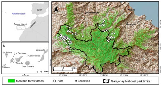
Figure 1.
Geographic situation of the Canary Islands (top left), La Gomera (bottom left), and the study area (right) with respective sample sites.
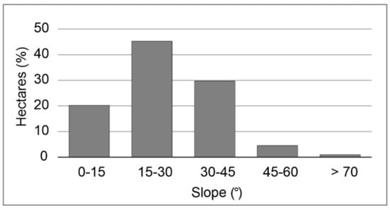
Figure 2.
Distribution of slope classes in the study area.
Laurel forests constitute a relict of the subtropical North Thetian forest from the end of the Tertiary era, which found refuge in the Macaronesia Islands after the Pleistocene glaciations [33]. It is the most diverse forest ecosystem of the Canary Islands, with a pluri-specific tree stratum of more than 20 evergreen broadleaf tree species. Most of these species belong to the family Lauraceae, but there are species from other families also present. The canopy height varies from < 5 m, in the fayal-brezal substitution thickets, to more than 30 m in the most humid and mature stands, distinguishing five potential vegetation communities according to meso-topoclimatic factors [33]: dry evergreen laurel forest (Visneo mocanerae-Arbutetum canariensis); humid evergreen laurel forest (Lauro novocanariensis-Perseetum indicae); cold evergreen laurel forest (Pericallido-Myricetum fayae); Erica platycodon ridge-crest evergreen forest (Ilici canariensis-Ericetum platycodonis); and hygrophilous evergreen laurel forest (Diplazio caudati-Ocoteetum foetentis).
2.2. Field Inventory
A total of 60 plots measuring 30 × 30 m (0.09 ha) were sampled along a forest development gradient during 2019. The forest development was assessed using aerial pictures from 2019 that were obtained from GRAFCAN S.L. [45]. We distinguished three plot types: open woodlands (OA, n = 10), with isolated trees and a canopy cover < 75%; young-growth forests (YGF, n = 22); and old-growth forests (OGF, n = 28), with greater canopy richness and larger crown sizes than in YGF [46]. Each plot was georeferenced in its centroid using GPS, with an error margin < 3 m. All sample plots were situated on hillside with slopes between 10° and 35°.
At each plot, the species, height, and diameter at breast height (DBH) were recorded for each individual adult tree (height ≥ 2 m and DBH ≥ 2.5 cm) and their suckers. We estimated aboveground biomass (AGB) at each stand (Mg. ha−1), using DBH and applying the specific allometric equations from Aboal et al. [47]. For those species without a specific formula, we used the general equation by Fernández-Palacios et al. [48]. DBH mean, basal area (m2 ha−1), and stem density (N. ha−1) per plot were also calculated. Vertical complexity was assessed using the Pielou index (J’) [49], with a rank of 5 m for each height class, starting at 2 m up to 37 m to obtain seven tree height categories [50] (Figure 3a).
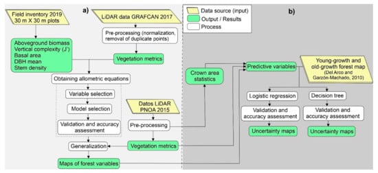
Figure 3.
Workflow diagram. (a) Development of allometric formulas of forest attributes. (b) Distinction between young-growth and old-growth laurel forests.
2.3. LiDAR Inventory
Large foot-print LiDAR data, used to build the allometric equations, was supplied by GRAFCAN S.L. [51]. The data was collected in 2017, the closest available data to the date of the field inventory. The mean point density within the study area averaged 2.6 points per m2 and four returns per laser pulse were recorded. The points were categorized following the classification defined by the American Society for Photogrammetry and Remote Sensing (ASPRS) for LAS formats (Figure 3a).
A second LiDAR dataset was acquired for the generalization of allometric formulas for all the laurel forest areas in La Gomera. Free access LiDAR data from the Spanish National Aerial Orthophotography Plan (PNOA) [52] were used. These data had very similar characteristics to data from 2017 and were acquired with a sensor LEICA ALS60 in 2015. The point density in the study area averaged 2.5 points per m2 and four returns per laser pulse were recorded. The points were also classified according to ASPRS (Figure 3a).
2.4. LiDAR Data Processing
There are two approaches to estimating forest structural attributes using LiDAR metrics. In the first approach, LiDAR metrics are obtained to stand or plot level with a single value by cell and variable, from the point clouds. The second approach applies LiDAR metrics from individual trees. For this purpose, it is necessary to identify each tree using point clouds and the biomass for each individual tree is estimated, then these data are aggregated at the stand scale.
Despite the individual trees approach resulting in higher accuracy [53,54,55,56], we used the first method due to the canopy and LiDAR data characteristics. Laurel forests have a closed canopy, and even though there are new techniques to delimit each tree [57,58], these use LiDAR clouds with greater points density. Furthermore, the pluri-specific canopy of laurel forest would require the species identification of each tree to apply the respective allometric equations.
The LiDAR metrics were performed using FUSION [59] software packages. We did a pre-processing to remove overlapped points, removing those that corresponded to the highest angle flight line. Then the ‘ground’ class was used to normalize the point elevation and to calculate the height above ground level. Normalized returns corresponding to each plot were clipped from the LiDAR dataset and several variables were derived from the height distribution of returns (Figure 3a). These variables (Table 1) were displayed as digital models with a pixel size of 30 × 30 m. The metrics were calculated using a 2-m threshold to remove all points below and avoid the inclusion of ground and low vegetation returns.

Table 1.
Metrics derived from the height distribution of LiDAR at each field plot and used as explanatory variables in models. Variables were computed from a minimum threshold of 2 m above ground.
2.5. Allometric Equations
Development of allometric equations was conducted using the 2017 LiDAR dataset and field data from 2019 (Figure 3a). The fact that there is a time lag of two years between both datasets could be a problem if the rate of change of forest is high. We should consider that laurel forest species do not have a very fast growth. Therefore, we assume that 2-year timespan would not imply significant differences in vegetation heights. In order to confirm this assumption, we previously analyzed the change in canopy height model (P95) and canopy cover, using LiDAR data from 2015 and 2017, and we tested if there are significant differences over a two-year period. The results of t-test and Willcoxon-test (Figure S1) with non-significant differences confirmed our assumption.
Standard linear regression, exponential regression, and generalized linear models (GLM) were the primary statistical methods applied to study the relation between field measurements and explanatory variables from LiDAR data. We chose the best fitted method to the dependent variable distribution.
All LiDAR metrics and the interaction (i.e., product) between them were used as explanatory variables on the models. In order to ensure normality and homocedasticity, the x values were transformed to natural log(x + 1), procedure that was applied to all variables. The three most meaningful predictors to each dependent variable were selected using the regsubset function (package “leaps”) [60] and we established a set of models ranging from one to three explanatory variables. Variance inflation factors (VIFs) were calculated to check multicollinearity among explanatory variables in each model, and those with VIFs greater than six were rejected. The end models were chosen according to the minimum corrected Akaike information criterion (AIC).
The chosen models were validated, and their residuals were analyzed checking the normality and homocedasticity. We used leave-one-out cross-validation method (loocv) of train function (package “caret”) [61], where a model is fitted using n-1 samples (n: total number of samples in the dataset). This process is repeated for each observation and a prediction error is calculated, obtaining R2, bias and root mean squared error (RMSE). Both, RMSE and bias were also calculated as percentage by and , where is the mean of field observed data.
These analyses were applied to all field measures distinguishing the three plot types separately (OW, YFG, and OGF) (Figure 4) and as a whole.
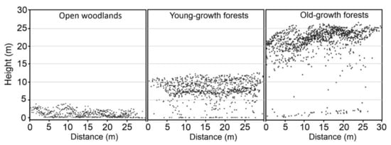
Figure 4.
Cross-section of 30 m in study plots. LiDAR data points cloud in three different laurel forest development stages are showed. Left to right: the initial stage, open woodlands; the intermediate stage of young-growth forest; and the end stage of old-growth forest.
The variables with best fit-goodness were used to create a wall-to-wall prediction of these variables on all laurel forests in La Gomera. The resulting maps were supervised based on aerial photography from 2015 [62]. We removed those cells (n = 22) with isolated presence of individuals of Pinus spp., Eucalyptus spp., and other exotic species, which clearly alter the forest metrics data.
All statistical calculations were performed with R [63] and the indicated packages.
2.6. Distinguishing Young-Growth and Old-Growth Laurel Forest
The usefulness of LiDAR for the recognition of both forest types was assessed. Two methods were applied: decision tree and logistic regression. Logistic regression is a nonlinear regression method for predicting a categorical output variable as in our case. The decision tree was implemented in R [63] using classification and regression trees (CART) algorithm, “rpart package” [64]. An upward pruning was applied, until a number of nodes with the lowest error rate was reached.
The predicted variables used were: AGB, basal area, vertical complexity (J’), DBH mean, and the relative height density computed for the seven height bins. Additionally, we calculated three variables about the tree crown area to each pixel (maximum, mean, and standard deviation) (Figure 3b), through a GIS-based individual tree crown delineation based following to Argamosa et al. [65]. The output variable (young-growth and old-growth forests) was obtained from a cartography in vector format (and transformed to raster format) at 1:5000 scale and elaborated from aerial photos by Del Arco and Garzón-Machado [46] (Figure 3b). We removed the burnt areas from the 2012 fire to avoid possible noise from these areas. The collinearity among variables was controlled, rejecting those that were highly correlated (Rho ≥ 0.75 and p < 0.5). In each pair of variables, we selected those with higher correlation with output variable.
From among the data, 70% were chosen randomly to create a training dataset, and the remaining 30% were used as a test dataset to predict values and evaluate the accuracy of both methods. The performance of both models was assessed through three evaluated indices for accuracy, sensitivity, and specificity. Accuracy measures the fraction of cases correctly classified. Sensitivity measures the proportion of positive cases that are classified as positive. Specificity measures the fraction of negative cases classified correctly.
where: TP—true positives; TN—true negatives; FP- false positives; and FN—false negatives. The models with the highest sensitivity, specificity, and accuracy are the best predictive models.
Accuracy = (TP + TN)/(TP + FP + TN + FN)
Sensitivity = TP/(TP + FN)
Specificity = TN/(FP + TN)
Additionally, ROC curves were built up and areas under the ROC curves (AUC) were identified. Uncertainty maps for both techniques were also developed to evaluate their performance in the evaluated territory (Figure 3b). The correlation between the errors of uncertainty maps and the slope were tested through Spearman correlation.
3. Results
3.1. Allometric Formulas
Field data reported stands with a mean vertical complexity (J´) of 0.39 and standard deviation (SD) of ± 0.21. The AGB reached maximums of around 500 Mg. ha−1 and a mean of 198.8 ± 19.3 Mg. ha−1. Basal area reached a maximum of 101 m2 ha−1 with a mean of 41.3 ± 3.1 m2 ha−1. Stem density had an average of 2525.3 ± 234.1 stems. ha−1, while the DBH mean reached a maximum value of 45.8 cm with a mean of 13.4 ± 1.1 cm (Figure 5).
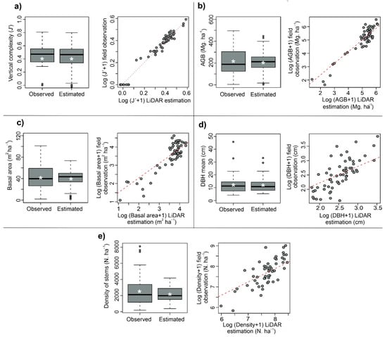
Figure 5.
Performance (left) and validation (right) graphs to each forest structure attribute studied. (a)Vertical complexity (J), (b) AGB, (c) basal area, (d) DBH mean, and (e) density of stems.
For all the structure variables analyzed, the models were best fitted using the whole plots than performing models to each stratum separately (OW, YGF, and OGF). The standard linear regression with double-log form was the best method for all cases. The vertical structure complexity (J´) was the variable with the best goodness-of-fit (R2 = 0.99, see Table 2), and lowest RMSE% and bias. The aboveground biomass model, by means of using the interaction between cover and P25 as input, also showed a high fit (R2 = 0.87). Basal area, DBH mean, and stem density showed a medium to high goodness-of-fit between the LiDAR metrics and field data, R2 ranging from 0.77 to 0.65 (Table 2). On the other hand, the estimates of the different structure measurements were always within the range of the values measured in the field (Figure 5).
Table 2.
Results of the best model for each forest structural attribute.
3.2. Mapping Structure Variables
The vertical complexity (J´) mean was 0.31 ± 0.26, ranging between 1.16 and −0.07, but if we rejected the two highest outliers, the maximum vertical complexity (J´)was 1.08 (Figure 6a and Figure S2). The AGB reported values between 641 and 0 Mg. ha−1 with an average of 132 ± 112.5 Mg. ha−1, again the maximum decrease until 571 Mg. ha−1 when the two highest outlier pixels were rejected (Figure 6b and Figure S3). The laurel forest from La Gomera would harbor a total AGB around 10 million of Mg. ha−1. Basal area ranged between 92.5 and −0.5 m2 ha−1 (Figure 6c) with a mean of 29.2 ± 18.9 m2 ha−1 (Figure S4). Respect to DBH mean, had a mean of 10.7 ± 6.2 cm, ranging from 0 to 40 cm (Figure 6d and Figure S5).
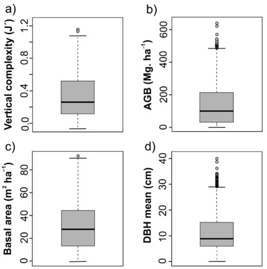
Figure 6.
Boxplots with the predicted values in the entirety of the laurel forests of La Gomera. (a) Vertical complexity (J’), (b) above-ground biomass, (c) basal area, and (d) DBH mean. The sample size to each variable was 73,370 pixels of 30 × 30 m.
3.3. Identifying Young-Growth and Old-Growth Laurel Forests through LiDAR
Logistic regression and tree decision had a very similar performance to distinguish YGF and OGF, with an accuracy, sensitivity, and specificity nearly identical with values around 0.8, which reveal a high to medium-high fit (Table 3). The ROC curve and AUC, showed also similar results (Figure 7).
Table 3.
Performance data of decision tree and logistic regression to discriminate between YGF and OGF.
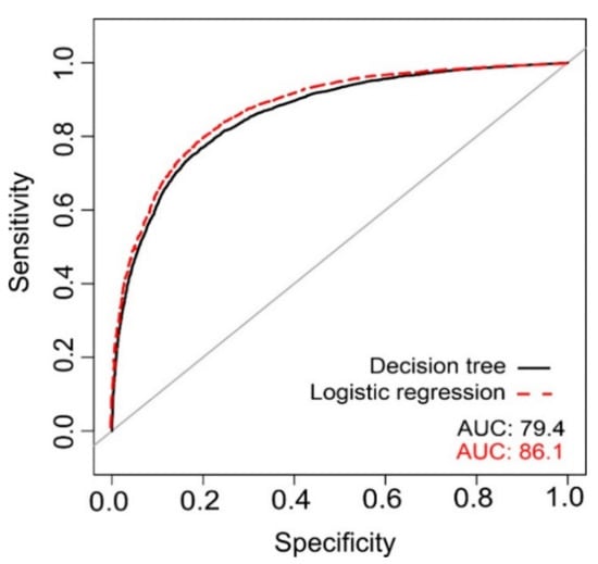
Figure 7.
ROC curve and AUC for decision tree and logistic regression.
The input variables introduced in both models, after controlling for collinearity, were D01, D02, D03, D04, D05, D06, vertical complexity (J’), mean tree crown area, and standard deviation of the tree crown area. The logistic regression showed significant p-values for D01, D02, D03, D04, and the vertical complexity (J’) (Table 4), while significant variables for the decision tree were vertical complexity (J’), D01 and mean tree crown area (Figure 8).
Table 4.
Parameters and p values of each of the input variables of the best logistic regression model to distinguish between YGF and OGF.
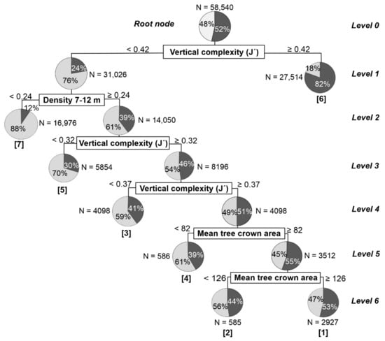
Figure 8.
Results of the decision tree to distinguish YGF (clear gray color) and OGF (dark gray color) stands. N is the sample size (pixels 30 × 30 m) in each node. The numbers in parentheses under each terminal node show the probability of discriminating between the two forest types from the lowest [1] to the highest [7] for those cases that reached the corresponding terminal nodes.
Uncertainty maps (Figures S6 and S7) showed that, for the decision tree, 72.8% of the pixels were classified correctly, underestimating the forest maturity in 25.2% of the cases, and overestimating it in 2% of cases. In contrast, the logistic regression was able to correctly classify 79.44% of the area, underestimating the forest maturity in 15% of the cases and overestimating it in 5.6% of cases. Tests showed correlation between the errors and slope, although with a very low Rho, Rho = −0.084, with p ≤ 0.001 for logistic regression, and Rho = −0.030, with p ≤ 0.001, for decision tree.
4. Discussion
For the first time, a whole set of equations for mapping the forest structure variables of Canarian laurel forests are available. Previous works have been carried out for the classification of communities [33] and forest maturity [46] using aerial photos in conjunction with fieldwork. Nevertheless, the characteristics that LiDAR offers to assess several variables of the forest structure through easily generalizable formulas, was an aspect that had not been evaluated before for the Canarian laurel forests.
The accuracy of our estimates was in accordance with other temperate and tropical forests. The R2 values were even higher than obtained for AGB [28,29,66] and DBH [28] using linear regression techniques. Nevertheless, RMSE data were somewhat high compared to elsewhere [18,28,29,66], although these errors were compensated for by low bias. These high RMSE could be related with a small plot size (0.09 ha) as has been pointed out by García et al. [18] and Frazer et al. [19], which showed that an increase in plot size improved the model accuracy, because it reduces the effect of registration errors between field and LiDAR data. However, we should bear in mind that the homogeneity of the forest structure is very important when considering the impact of plot size on model accuracy, with different optimum sizes for each forest type [19,20]. Although the phases of young growth laurel forests have a relatively homogeneous structure, old-growth forests have a heterogeneous and multi-species structure with the presence of many micro-gaps [38]. This, together with historical human exploitation and the complex topography of the Canaries, would discourage the use of maximum plot size usually applied in similar works (1 ha). For this reason, we believe it would be convenient to carry out new studies in the laurel forest to evaluate the effect of plot size on the performance of the models, in order to obtain an ideal size of the sampling plot for this forest. To improve model accuracy in heterogeneous forests, several studies had used the canopy cover for AGB predictions [18,21,22,23], as has also occurred in our case. Another aspect influencing AGB accuracy is the point cloud density as has been demonstrated by García et al. [18], where densities below 5 points increased the RMSE model.
AGB estimation models usually had included the 50th percentile or average height [18,62], but as in our study, the use of other height metrics such as the 10th or 90th percentile have been equally valid [28,67]. Vertical complexity has always been a difficult variable to measure in the field. In contrast, many LiDAR studies take height standard deviation of points as a simple way of measuring vertical complexity [10], but without contrasting to the field data of vertical complexity. Here, vertical complexity was measured in the field through the Pielou Index, but the best explanatory metric was not the height standard deviation of the point clouds, but rather the average height of point cloud and the point density in the first height bin (2–7 m). Thus, we found evidence that standard deviation of the height points will not always be the best metric to estimate vertical complexity, especially in closed canopy forests where the detection of understory vegetation is more difficult.
Vertical complexity, followed by the points density in the height bin of 7–12 m height, were the most important explanatory variables for the identification of YGFs and OGFs, according to the two methods applied. Additionally, point density in other height bins was also included in the logistic regression, while was the tree crown area in the decision tree. These results would agree with the existing knowledge about these forests, where the vertical complexity has already been pointed out as one of the most correlated variables with the forest maturity [38,68]. The point density of the height bin 7–12 m, would be highly related with the canopy height, distinguishing a large area of the YGFs that have a height below to 7–12 m with this variable [38]. The tree crown area in recognition of both forest types is also worth noting, with an abundance of large trees in mature forest areas [38,69].
As has already been mentioned, the use of field and LiDAR data at different dates (2 years) could be a problem, if the vegetation growth in that period of time is significant enough. Although it is ideal to have field and LiDAR data from the same year, the applied tests revealed that in 2 years there are not significant differences in canopy height for the laurel forest. In general, the species that compose it do not have a very fast growth, and it is necessary more than 140 years for these forests to reach a structural maturity [38]. Complementarily, most of this territory is within the National Park and other protected natural areas, and these forests have been included in the European Red List of Habitats [70], so that human exploitation and the evolution of the landscape is not an aspect that can affect the estimation of the heights and volumes of this forest.
In this study, priority was given to the equations design of simple application and generalization to the whole of laurel forest, offering continuous data across all forest cover. It is certain that local variations of soil, topography, and climate influence the maximum potential of heights and AGB that can be reached by a forest stand [71,72,73]. For this reason, we used field data from plots located on hillside situations, the most generalized topographic situation, located in middle areas between ridges and bottom-valleys. Likewise, the thresholds of the forest structure variables used to delimit the young-growth and old-growth forests could change slightly depending on the vegetation community—e.g., these would be lower in dry laurel forests than humid or bottom-valley laurel forests. Therefore, we consider it convenient to develop new allometric formulas specific to each vegetation community, based on the separate field data of each community.
Uncertainty maps of forest maturity revealed that the models developed (logistic regression and decision tree) tend to underestimate maturity in areas with steep slopes, with a high correlation between slope and error in both techniques, especially decision tree, which showed worse results than logistic regression. The effect of steep slopes on estimates of vegetation heights and volumes has been described in several previous works [11,24,25], developing statistical approaches that allow incorporating the slope and controlling its effect. This will be a very important aspect to take into account in future LiDAR work in this forest, because much of the Canarian laurel forest is located on areas with steep slopes. Thus, the development of these new approaches will allow for better control the effect of slope. On the other hand, the use of SAR images in combination with LiDAR has shown good results [16], especially to correct negative effects of topography, so its use in this case could be very useful.
In the analyses, we have assumed the spatial independence of the pixels/plots, but we know that in forest studies this is not usually the case. Spatially, in our case, we have prioritized a stratified sampling (plots with different forest stage) over a systematic sampling in order to have as much variance as possible. Obtaining semivariogram functions and their inclusion in the allometric formulas to determine forest heights and volumes would undoubtedly improve the reliability of the formulas presented here.
Though forest structure is a key factor in the forest maturity concept, it should not be the only one. We agree with many authors that definition of maturity should be accompanied by other ecological aspects such as species composition [1,74] and microhabitat diversity [38,75,76]. It is important to not forget this when visualizing the data presented here.
Here, we have shown for the first-time using LiDAR the structural reality of the entirety of the laurel forests in La Gomera, which have been scarcely applied to these forests before now. The results obtained indicate that this remote sensing technique can be a useful tool for Macaronesian laurel forest monitoring, despite it being a closed canopy forest. However, its potentiality can be improved by using LiDAR datasets with a higher density of points and by developing new allometric formulas for the different vegetation communities.
5. Conclusions
For the first time, a set of allometric formulas are available for LiDAR use in the Macaronesian laurel forest. LiDAR showed its potentiality on these forests, showing linear regression a good performance for the calculation of vertical complexity and AGB. It also had the ability to correctly distinguish between young-growth and old-growth forest encompassing the range of 70–80% of the cases. However, we detected a number of problems in its application, mainly related to the control of the effect of relief that should be further studied in future work in order to obtain better equations.
Supplementary Materials
The following supporting information can be downloaded at: https://www.mdpi.com/article/10.3390/rs14040994/s1, Figure S1: Boxplots of LiDAR 2017 and 2015 datasets in the studied plots. A comparison of canopy height model (m) and canopy cover (%); Figure S2: Map of estimation of the vertical complexity (J’); Figure S3: Map of estimation of the above-ground biomass (Mg. ha−1); Figure S4: Map of estimation of the basal area (m2 ha−1); Figure S5: Map of estimation of the DBH mean (cm); Figure S6: Uncertainty map using decision tree; Figure S7: Uncertainty map using logistic regression.
Author Contributions
Conceptualization, J.P.-D. and Á.B.F.L.; Methodology, J.P.-D.; Validation, J.P.-D., Á.B.F.L. and J.M.G.-M.; Formal analysis, J.P.-D.; Investigation, J.P.-D.; Resources, J.P.-D., Á.B.F.L., and L.A.G.G.; Writing—original draft preparation, J.P.-D. and J.M.G.-M.; Writing—review and editing, J.P.-D., Á.B.F.L., L.A.G.G., M.J.d.A.A. and J.M.G.-M.; Visualization, J.P.-D.; Supervision, Á.B.F.L. and J.M.G.-M. All authors have read and agreed to the published version of the manuscript.
Funding
This research was funded by ‘Agencia Canaria de Investigación, Innovación y Sociedad de la Información’ of the Canary Islands Government through their program of financial support for researchers cofounded in 85% by the European Social Fund (ESF). The APC was co-funded by La Laguna University through of the research staff training program.
Institutional Review Board Statement
Not applicable.
Informed Consent Statement
Not applicable.
Data Availability Statement
LiDAR dataset from 2017 was purchased from GRAFCAN S.L. through its online-shop (http://tiendavirtual.grafcan.es/visor.jsf?currentSeriePk=340230144, accessed on 10 February 2021). LiDAR dataset from 2015 was obtained from the Spanish National Geographic Institute (IGN) (http://centrodedescargas.cnig.es/CentroDescargas/catalogo.do?Serie=LIDAR, accessed on 10 February 2021).
Acknowledgments
We are grateful to Victor Bello and Jonay Cubas for their assistance in fieldwork; as well as to Zachary Schmidt for his help with the English review.
Conflicts of Interest
The authors declare no conflict of interest.
References
- Lindenmayer, D. Forest Pattern and Ecological Process: A Synthesis of 25 Years of Research; CSIRO Publishing: Clayton, Australia, 2009; p. 320. [Google Scholar] [CrossRef]
- FAO. The State of the World´s Forests (SOFO); FAO: Rome, Italy; p. 139. Available online: http://www.fao.org/3/i9535en/i9535en.pdf (accessed on 22 May 2021).
- Roy, J.; Saugier, B.; Mooney, H.A. Terrestrial Global Productivity; Academic Press: San Diego, CA, USA, 2001; p. 573. [Google Scholar]
- Mackey, B.; Prentice, I.C.; Steffen, W.; House, J.I.; Lindenmayer, D.; Keith, H.; Berry, S. Untangling the confusion around land carbon science and climate change mitigation policy. Nat. Clim. Chang. 2013, 3, 552–557. [Google Scholar] [CrossRef]
- Gillespie, T.W.; Foody, G.M.; Rocchini, D.; Giorgi, A.P.; Saatchi, S. Measuring and modeling biodiversity from space. Progr. Phys. Geogr. 2008, 32, 203–221. [Google Scholar] [CrossRef]
- Baldeck, C.A.; Asner, G.P. Estimating vegetation beta diversity from airborne imaging spectroscopy and unsupervised clustering. Remote Sens. 2013, 5, 2057–2071. [Google Scholar] [CrossRef] [Green Version]
- Zhou, Z.; Liu, R.; Shi, S.; Su, Y.; Li, W.; Guo, Q. Ecological niche modeling with LiDAR data: A case study of modeling the distribution of fisher in the southern Sierra Nevada Mountains, California. Biodivers. Sci. 2018, 26, 878–891. [Google Scholar] [CrossRef]
- Knyazikhin, Y.; Kranigk, J.; Myneni, R.B.; Panfyorov, O.; Gravenhorst, G. Influence of small-scale structure on radiative transfer and photosynthesis in vegetation cover. J. Geophys. Res. 1998, 103, 6133–6144. [Google Scholar] [CrossRef]
- Potter, C.; Tan, P.; Steinbach, M.; Klooster, S.; Kumar, V.; Myneni, R.; Genovese, V. Major disturbance events in terrestrial ecosystems detected using global satellite data sets. Glob. Chang. Biol. 2003, 9, 1005–1021. [Google Scholar] [CrossRef] [Green Version]
- Coops, N.C.; Tompaski, P.; Nijland, W.; Rickbeil, G.J.M.; Nielsen, S.E.; Bater, C.W.; Stadt, J.J. A forest structure habitat index based on airborne laser scanning data. Ecol. Indic. 2016, 67, 346–357. [Google Scholar] [CrossRef]
- Muhammad, A.; Mengjiado, Y.; Rasheed, A.; Jin, X.; Xia, X.; Xiao, Y.; He, Z. Time-Series Multispectral Indices from Unmanned Aerial Vehicle Imagery Reveal Senescence Rate Wheat. Remote Sens. 2018, 10, 809. [Google Scholar] [CrossRef] [Green Version]
- Underwood, E.; Ustin, S.; Di Pietro, D. Mapping nonnative plants using hyperspectral imagery. Remote Sens. Environ. 2003, 86, 150–161. [Google Scholar] [CrossRef]
- Mitchell, J.; Glenn, N.F. Leafy Spurge (Euphorbia esula L.) classification performance using hyper-spectral and multispectral sensors. Rangel. Ecol. Manag. 2009, 62, 16–27. [Google Scholar] [CrossRef]
- Sun, G.; Ranson, J. Forest biomass retrieval from lidar and radar. In Proceedings of the IEEE International Geoscience and Remote Sensing Symposium, Cape Town, South Africa, 12–17 July 2009. [Google Scholar]
- Kaasalainenm, S.; Holopainen, M.; Karjalainen, M.; Vastaranta, M.; Kankare, V.; Karila, K.; Osmanoglu, B. Combining Lidar and Synthetic Aperture Radar Data to Estimate Forest Biomass: Status and Prospects. Forests 2015, 6, 252–270. [Google Scholar] [CrossRef]
- Tanase, M.A.; Panciera, R.; Lowell, K.; Aponte, C.; Hacker, J.M.; Walker, J.P. Forest Biomass Estimation at High Spatial Resolution: Radar Versus Lidar Sensors. IEEE Geosci. Remote Sens. Lett. 2014, 11, 711–715. [Google Scholar] [CrossRef]
- Huang, W.; Sun, G.; Dubayah, R.; Cook, B.; Montesano, P.; Ni, W.; Zhang, Z. Mapping biomass change after forest disturbance: Applying LiDAR footprint-derived models at key map scales. Remote Sens. Environ. 2013, 134, 319–332. [Google Scholar] [CrossRef]
- García, M.; Saatchi, S.; Ferraz, A.; Silva, C.A.; Ustin, S.; Koltunov, A.; Balzter, H. Impact of data model and point density on aboveground forest biomass estimation from airborne LiDAR. Carbon Balance Manag. 2017, 12, 4. [Google Scholar] [CrossRef] [PubMed] [Green Version]
- Frazer, G.W.; Magnussen, S.; Wulder, M.A.; Niemann, K.O. Simulated impact of sample plot size and co-registration error on the accuracy and uncertainty of LiDAR-derived estimates of forest stand biomass. Remote Sens. Environ. 2011, 115, 636–649. [Google Scholar] [CrossRef]
- Mascaro, J.; Detto, M.; Asner, G.P.; Muller-Landau, H.C. Evaluating uncertainty in mapping forest carbon with airborne Lidar. Remote Sens. Environ. 2011, 115, 3770–3774. [Google Scholar] [CrossRef]
- Hall, S.A.; Burke, I.C.; Box, D.O.; Kaufmann, M.R.; Stoker, J.M. Estimating stand structure using discrete-return lidar: An example from low density, fire prone ponderosa pine forests. Ecol. Manag. 2005, 208, 189–209. [Google Scholar] [CrossRef]
- Næsset, E.; Gobakken, T. Estimation of above- and below-ground biomass across regions of the boreal forest zone using airborne laser. Remote Sens. Environ. 2008, 112, 3079–3090. [Google Scholar] [CrossRef]
- García, M.; Riaño, D.; Chuvieco, E.; Danson, F.M. Estimating biomass carbon stocks for a Mediterranean forest in Spain using height and intensity LiDAR data. Remote Sens. Environ. 2010, 114, 816–830. [Google Scholar] [CrossRef]
- Rosette, J.A.B.; North, P.R.J.; Suarez, J.C.; Los, S.O. Uncertainty within satellite LiDAR estimations of vegetation and topography. Int. J. Remote Sens. 2010, 31, 1325–1342. [Google Scholar] [CrossRef]
- Yang, W.; Ni-Meister, W.; Lee, S. Assessment of the impacts of surface topography, off-nadir pointing and vegetation structure on vegetation lidar waveforms using an extended geometric optical and radiative transfer model. Remote Sens. Environ. 2011, 115, 2810–2822. [Google Scholar] [CrossRef]
- Zhao, F.; Guo, Q.; Kelly, M. Allometric equation choice impacts lidar-based forest biomass estimates: A case study from the Sierra National Forest, CA. Agric. For. Meteorol. 2012, 165, 64–72. [Google Scholar] [CrossRef]
- Sheridan, R.; Popescu, S.; Gatziolis, D.; Morgan, C.; Ku, N.-W. Modeling Forest Aboveground Biomass and Volume Using Airborne LiDAR Metrics and Forest Inventory and Analysis Data in the Pacific Northwest. Remote Sens. 2014, 7, 229–255. [Google Scholar] [CrossRef]
- Teobaldelli, M.; Cona, F.; Saulino, L.; Migliozzi, A.; D’Urso, G.; Langella, G.; Manna, P.; Saracino, A. Detection of diversity and stand parameters in Mediterranean forests using leaf-off discrete return LiDAR data. Remote Sens. Environ. 2017, 192, 126–138. [Google Scholar] [CrossRef]
- Borges, P.A.V.; Cardoso, P.; Kreft, H.; Whittaker, R.J.; Fattorini, S.; Emerson, B.C.; Gil, A.; Gillespie, R.G.; Matthews, T.J.; Santos, A.M.C.; et al. Global Island Monitoring Scheme (GIMS): A proposal for the long-term coordinated survey and monitoring of native island forest biota. Biodivers. Conserv. 2018, 27, 2567–2586. [Google Scholar] [CrossRef] [Green Version]
- Whittaker, R.J.; Fernández-Palacios, J.M.; Matthews, T.J.; Borregaard, M.K.; Triantis, K.A. Island biogeography: Taking the long view of natures laboratories. Science 2017, 357, eaam8326. [Google Scholar] [CrossRef] [Green Version]
- Mittermeier, R.A.; Robles, G.; Hoffman, M.; Pilgrim, J.; Brooks, T.; Mittermeier, C.G.; Lamoreux, J.; Fonseca, G.A.B. Hotspots Revisited: Earth’s Biologically Richest and Most Endangered Terrestrial Ecoregions; University of Chicago Press: Boston, MA, USA, 2005; p. 392. [Google Scholar]
- Nerelli, G.; Fernández-Palacios, J.M. Análisis de los servicios prestados por los ecosistemas a las comunidades humanas. El caso del monteverde gomero y del pinar grancanario. Boletín De La Real Soc. Económica De Amigos Del País De Tenerife 2010, 1, 237–250. [Google Scholar]
- Del Arco, M.J.; González-González, R.; Garzón-Machado, V.; Pizarro-Hernández, B. Actual and potential natural vegetation on the Canary Islands and its conservation status. Biodivers. Conserv. 2010, 19, 3089–3140. [Google Scholar] [CrossRef]
- Kondraskov, P.; Schütz, N.; Schüßler, C.; Menezes de Sequeira, M.; Guerra, A.S.; Caujapé-Castells, J.; Jaén-Molina, R.; Marrero-Rodríguez, Á.; Koch, M.A.; Linder, P.; et al. Biogeography of Mediterranean Hotspot Biodiversity: Re-Evaluating the “Tertiary Relict” Hypothesis of Macaronesian Laurel Forests. PLoS ONE 2015, 10, e0132091. [Google Scholar] [CrossRef]
- Mairal, M.; Caujapé-Castells, J.; Pellissier, L.; Jaén-Molina, R.; Álvarez, N.; Heuertz, M.; Sanmartín, I. A tale of two forests: Ongoing aridification drives population decline and genetic diversity loss at continental scale in Afro-Macaronesian evergreen-forest archipelago endemics. Ann. Bot. 2018, 122, 1005–1017. [Google Scholar] [CrossRef]
- Otto, R.; Garzón-Machado, V.; Del Arco, M.J.; Fernández-Lugo, S.; de Nascimento, L.; Oromí, P.; Báez, M.; Ibáñez, M.; Alonso, M.R.; Fernández-Palacios, J.M. Unpaid extinction debts for endemic plants and invertebrates as a legacy of habitat loss on oceanic islands. Divers. Distrib. 2017, 23, 1031–1041. [Google Scholar] [CrossRef] [Green Version]
- Marrero, M.C.; Marrero, M.V.; Carqué, E.; Bañares, A.; Fernández, A.; Ojeda, E.; Hernández-Luis, A.; Afonso, L.; Acevedo, A. Euphorbia mellifera Aiton. In Atlas y Libro Rojo de la Flora Vascular Amenazada de España. Taxones Prioritarios; Bañares, A., Blanca, G., Güemes, J., Moreno, J.C., Ortiz, S., Eds.; Dirección General de Conservación de la Naturaleza: Madrid, Spain, 2004; pp. 256–257. [Google Scholar]
- Fernández, Á.B.; Gómez, L.A. Qué son los bosques antiguos de laurisilva. Su valor y situación en Canarias. In La Gomera, Entre Bosques y Taparuchas; Afonso-Carrillo, J., Ed.; Instituto de Estudios Hispánicos de Canarias: Tenerife, Spain, 2016; pp. 177–236. [Google Scholar]
- Núñez-Casillas, L.; Micand, F.; Somers, B.; Brito, P.; Arbelo, M. Plant species monitoring in the Canary Islands using WorldView-2 imagery. In Proceedings of the XXI International Society for Photogrammetry and Remote Sensing Congress, Melbourne, Australia, 9 January–8 May 2012. [Google Scholar]
- Martín-Luis, A.; Arbelo, M.; Hernánde-Leal, P.; Arbelo-Bayó, M. Mapping species distribution of Canarian Monteverde forest by field spectroradiometry and satellite imagery. In Proceedings of the SPIE Remote Sensing, Edinburg, UK, 25 October 2016. [Google Scholar] [CrossRef]
- Massetti, A.; Menezes de Sequeira, M.; Pupo, A.; Figueiredo, A.; Guiomar, N.; Gil, A. Assessing the effectiveness of RapidEye multispectral imagery for vegetation mapping in Madeira Island (Portugal). Eur. J. Remote Sens. 2016, 49, 643–672. [Google Scholar] [CrossRef] [Green Version]
- Devkota, R.S.; Field, R.; Hoffmann, S.; Walentowitz, A.; Medina, F.M.; Vetaas, O.R.; Chiarucci, A.; Weiser, F.; Jentsch, A.; Beierkuhnlein, C. Assessing the potential replacement of laurel forest by a novel ecosystem in the steep terrain of an Oceanic Island. Remote Sens. 2020, 12, 4013. [Google Scholar] [CrossRef]
- GRAFCAN and Agresta. Elaboración de cartografía de modelos de Combustibles Forestales. 2015. Available online: https://opendata.sitcan.es/dataset/modelos-de-combustible-forestales-de-canarias (accessed on 10 February 2021).
- Guillen-Climent, M.L.; Fernández-Landa, A.; Tomé, J.L.; Ranz, P.P. Análisis del estado de las masas forestales quemadas en el Parque Nacional de Garajonay (La Gomera) mediante el uso de técnicas de teledetección, sensores ópticos y LiDAR. In Proceedings of the XVI Congreso de la Asociación Española de Teledetección, Sevilla, Spain, 21–23 October 2015. [Google Scholar]
- GRAFCAN. WMS Service. OrtoExpress Año 2019. Available online: https://idecan1.grafcan.es/ServicioWMS/Historico/Ortofotos/OrtoExpress_2019? (accessed on 10 March 2021).
- Del Arco, M.J.; Garzón-Machado, V. Mapa del estado de la vegetación del Parque Nacional de Garajonay en el año 1951 y comparación con el estado actual. 2010; Unpublished document. [Google Scholar]
- Aboal, J.R.; Arévalo, J.R.; Fernández, Á. Allometric relationships of different tree species and stand above ground biomass in the Gomera laurel forest (Canary Islands). Flora 2005, 200, 264–274. [Google Scholar] [CrossRef]
- Fernández-Palacios, J.M.; García, J.J.; López Esteban, R.J.; Luzardo, M.C. Aproximación a la estima de la biomasa y producción neta aéreas en una estación de la Laurisilva tinerfeña. Vieraea 1991, 20, 11–20. [Google Scholar]
- Pielou, E.C. An introduction to Mathematical Ecology; Wiley Interscience: New York, NY, USA, 1969; p. 286. [Google Scholar]
- Bello-Rodríguez, V.; Gómez, L.A.; Fernández López, Á.; Del-Arco-Aguilar, M.J.; Hernández-Hernández, R.; Emerson, B.; González-Mancebo, J.M. Short- and long-term effects of fire in subtropical cloud forests on an oceanic island. Land Degrad. Dev. 2019, 30, 448–458. [Google Scholar] [CrossRef]
- GRAFCAN. Tienda Virtual. Datos LiDAR. Available online: http://tiendavirtual.grafcan.es/visor.jsf?currentSeriePk=340230144 (accessed on 10 February 2021).
- Instituto Geográfico Nacional (IGN). Plan Nacional de Ortofotografía Aérea (PNOA). LiDAR 2ª Cobertura (2015-Actualidad). Available online: http://centrodedescargas.cnig.es/CentroDescargas/catalogo.do?Serie=LIDAR (accessed on 10 February 2021).
- Hyyppä, J.; Kelle, O.; Lehikoinen, M.; Inkinen, M. A segmentation-based method to retrieve stem volume estimates from 3-D tree height model produced by laser scanners. IEEE Trans. Geosci. Remote Sens. 2001, 39, 969–975. [Google Scholar] [CrossRef]
- Persson, A.; Holmgren, J.; Södermann, U. Detecting and measuring individual trees using an airborne laser scanner. Photogram. Eng. Remote Sens. 2002, 68, 925–932. [Google Scholar]
- Popescu, S.C.; Wynne, R.H.; Nelson, R.E. Measuring individual tree crown diameter with lidar and assessing its influence on estimating forest volume and biomass. Can. J. Remote Sens. 2003, 29, 564–577. [Google Scholar] [CrossRef]
- Kwak, D.A.; Lee, W.K.; Lee, J.H.; Biging, G.S.; Gong, P. Detection of individual trees and estimation of tree height using lidar data. J. For. Res. 2007, 12, 425–434. [Google Scholar] [CrossRef]
- Ferraz, A.; Saatchi, S.; Mallet, C.; Jacquemoud, S.; Gonçalves, G.; Silva, C.A.; Soares, P.; Tomé, M.; Pereira, L. Airborne lidar estimation of aboveground forest biomass in the absence of field inventory. Remote Sens. 2016, 8, 653. [Google Scholar] [CrossRef] [Green Version]
- Khorrami, R.; Naeimi, Z.; Tabari, M.; Eslahchi, M.R. A new method for detecting individual trees in aerial LiDAR point clouds using absolute height maxima. Environ. Monit. Assess. 2018, 190, 1–16. [Google Scholar] [CrossRef]
- McGaughey, R.J. FUSION/LDV: Software for LIDAR Data Analysis and Visualization; U.S. Department of Agriculture, Forest Service: Seattle, WA, USA, 2014. [Google Scholar]
- Lumley, T.; Miller, A. Package ‘Leaps’. CRAN Repository. 2020. Available online: https://cran.r-project.org/web/packages/leaps/leaps.pdf (accessed on 15 April 2021).
- Kuhn, M.; Wing, J.; Weston, S.; Williams, A.; Keefer, C.; Engelhardt, A.; Cooper, T.; Mayer, Z.; Kenkel, B.; Benesty, M.; et al. Package ‘caret’. 2021. Available online: https://cran.r-project.org/web/packages/caret/caret.pdf (accessed on 15 April 2021).
- GRAFCAN. WMS Service. OrtoExpress Año 2015. Available online: https://idecan1.grafcan.es/ServicioWMS/Historico/Ortofotos/OrtoExpress_2015? (accessed on 10 February 2021).
- R Core Team. R: A Language and Environment for Statistical Computing; R Foundation for Statistical Computing: Vienna, Austria, 2020; Available online: https://www.R-project.org/ (accessed on 5 April 2021).
- Therneau, T.; Atkinson, B.; Ripley, B. Package ‘rpart’. CRAN Repository. 2019. Available online: https://cran.r-project.org/web/packages/rpart/rpart.pdf (accessed on 20 April 2021).
- Argamosa, R.J.L.; Paringit, E.C.; Quinton, K.R.; Tandc, F.A.M.; Faelga, R.A.G.; Ibañez, C.A.G.; Posilero, M.A.V.; Zaragosa, G.P. Fully automated GIS-Based individual tree Crown delineation based on curvature values from a LiDAR derived canopy height model in a coniferous plantation. In Proceedings of the XXIII International Society for Photogrammetry and Remote Sensing Congress, Prague, Czech Republic, 12–19 July 2016. [Google Scholar]
- Montesano, P.M.; Cook, B.D.; Sun, G.; Simard, M.; Nelson, R.F.; Ranson, K.J.; Zhang, Z.; Luthcke, S. Achieving accuracy requirements for forest biomass mapping: A spaceborne data fusion method for estimating forest biomass and LiDAR sampling error. Remote Sens. Environ. 2013, 130, 153–170. [Google Scholar] [CrossRef]
- Naesset, E.; Gobakken, T.; Solberg, S.; Gregoire, T.G.; Nelson, R.; Ståhl, G.; Weydahl, D. Model-assisted regional forest biomass estimation using LiDAR and InSAR as auxiliary data: A case study from a boreal forest area. Remote Sens. Environ. 2011, 115, 3599–3614. [Google Scholar] [CrossRef]
- Parada-Díaz, J.; Kluge, J.; Bello-Rodriguez, V.; Del Arco, M.J.; González-Mancebo, J.M. To what extent does the species composition of Macaronesian laurel forests depend on their human disturbance history and environmental drivers? For. Ecol Manag. 2021, 497, 119468. [Google Scholar] [CrossRef]
- Fernández-Palacios, J.M.; Arévalo, J.R.; Balguerías, E.; Barone, R.; de Nascimento, L.; Delgado, J.D.; Elías, R.B.; Fernández-Lugo, S.; Méndez, J.; Menezes de Sequeira, M.; et al. La Laurisilva: Canarias, Madeira y Azores; Macaronesia Editorial: Santa Cruz de Tenerife, Spain, 2017; p. 412. [Google Scholar]
- Janssen, J.A.M.; Rodwell, J.S.; García Criado, M.; Gubbay, S.; Haynes, T.; Nieto, A.; Sanders, N.; Landucci, F.; Loidi, J.; Ssymank, A.; et al. European Red List of Habitats. Part 2. Terrestrial and Freshwater Habitats; Publication Office of the European Union: Luxembourg, 2016. [Google Scholar]
- Asner, P.G.; Hughes, R.F.; Varga, T.A.; Knapp, D.E.; Kennedy-Bowdoin, T. Environmental and biotic controls over aboveground biomass throughout a tropical rain forest. Ecosystems 2009, 12, 261–278. [Google Scholar] [CrossRef]
- Ledo, A.; Illian, J.B.; Schnitzer, S.A.; Wright, S.J.; Dalling, J.W.; Burslem, D.F.R.P. Lianas and soil nutrients predict fine-scale distribution of above-ground biomass in a tropical moist forest. J. Ecol. 2016, 104, 1819–1828. [Google Scholar] [CrossRef] [Green Version]
- Muscarella, R.; Kolyaie, S.; Morton, D.C.; Zimmerman, J.K.; Uriarte, M. Effects of topography on tropical forest structure depend on climate context. J. Ecol. 2019, 108, 145–159. [Google Scholar] [CrossRef]
- Galen, L.G.; Jordan, G.J.; Musk, R.A.; Beeton, N.J.; Wardlaw, T.J.; Baker, S.C. Quantifying floristic and structural forest maturity: An attribute-based method for wet eucalypt forests. J. Appl. Ecol. 2018, 55, 1668–1681. [Google Scholar] [CrossRef]
- Courbaud, B.; Pupin, C.; Letort, A.; Cabanettes, A.; Larrieu, L. Modelling the probability of microhabitat formation on trees using cross-sectional data. Methods Ecol. Evol. 2017, 8, 1347–1359. [Google Scholar] [CrossRef] [Green Version]
- Patiño, J.; Gómez-Rodríguez, C.; Pupo-Correia, A.; Menezes de Sequeira, M.; Vanderpoorten, A. Trees as habitat islands: Temporal variation in alpha and beta diversity in epiphytic laurel forest bryophyte communities. J. Biogeogr. 2018, 45, 1727–1738. [Google Scholar] [CrossRef]
Publisher’s Note: MDPI stays neutral with regard to jurisdictional claims in published maps and institutional affiliations. |
© 2022 by the authors. Licensee MDPI, Basel, Switzerland. This article is an open access article distributed under the terms and conditions of the Creative Commons Attribution (CC BY) license (https://creativecommons.org/licenses/by/4.0/).