Abstract
Recognition of invasive species and their distribution is key for managing and protecting native species within both natural and man-made ecosystems. Small woody features (SWF) represent fragmented patches or narrow linear tree features that are of high importance in intensively utilized agricultural landscapes. Simultaneously, they frequently serve as expansion pathways for invasive species such as black locust. In this study, Sentinel-2 products, combined with spatiotemporal compositing approaches, are used to address the challenge of broad area black locust mapping at a high granularity. This is accomplished by conducting a comprehensive analysis of the classification performance of various compositing approaches and multitemporal classification settings throughout four vegetation seasons. The annual, seasonal (bi-monthly), and monthly median values of cloud-masked Sentinel-2 reflectance products are aggregated and stacked into varied time-series datasets per given year. The random forest algorithm is trained and output classification maps validated based on field-based reference datasets across Danubian lowlands (Slovakia). The main results of the study proved the usefulness of spatiotemporal compositing of Sentinel-2 products for mapping black locust in small woody features across wide area. In particular, temporally aggregated monthly composites stacked to seasonal time series datasets yielded consistently high overall accuracies ranging from 89.10% to 91.47% with balanced producer’s and user’s accuracies for each year’s annual series. We presume that a similar approach could be used for a broader scale species distribution mapping, assuming they are spectrally or phenologically distinctive, as is often the case for many invasive species.
1. Introduction
Native ecosystems as well as the goods and services that they provide are threatened by biological invasions, both in man-made and natural ecosystems. The black locust (Robinia pseudoacacia) is an alien invasive species of global importance [1]. Its native range lies in the eastern part of North America and, besides Europe, it is also naturalized in temperate South America, northern and southern Africa, temperate Asia, Australia, and New Zealand [2]. The black locust was introduced to Europe as early as the first half of the 17th century [2,3]. Due to its extensive planting since the late 18th and early 19th century (firewood, timber, erosion control) and dispersal ability, it colonized climatically suitable areas of Europe in the past, and now it belongs to the most widely distributed alien tree species in Europe.
The legume Robinia pseudoacacia (Fabaceae family) can fix nitrogen from the atmosphere and enrich the soil nitrogen with the aid of its symbiotic bacteria Therefore, only species that prefer or tolerate high nitrogen content in the soil can survive in the black locust-dominated plant communities. This has a detrimental effect on invaded habitats, reducing their diversity and natural character and resulting in the formation of species-poor communities. This process is linked with the extinction of many endangered light-demanding plants and invertebrates due to changes in light regime, microclimate, and soil conditions [3,4]. As a result, black locust canopies dramatically limit the natural variety of the agricultural landscape, reducing its potential to supply certain ecosystem services. Additionally, black locust can provide new habitats for other invasive species, such as its pest gall midge (Obolodiplosis robinia), which has invasively expanded its territory across Europe since its detection in 2003 in Italy [5], together with its parasitoid, Platygaster robiniae [6]. On the other hand, black locust stands contribute significantly to the greening of the Slovak intensive agricultural landscape, controlling soil erosion and supplying dendromass for forestry and habitats for beekeepers, demonstrating its contradictory impact on some ecosystem services. Small woody features represent critical greening elements in the intensive agricultural landscape [7]. The recent European High Resolution Layer (HRL) product of the EU program Copernicus (https://land.copernicus.eu/pan-european/high-resolution-layers, accessed on 10 October 2018) has been recently used for large scale assessment of ecosystem services, e.g., pest protection services [8]. Precise estimations of the distribution of black locusts within SWF (small woody features) can aid in our understanding and assessment of ecosystem services across a broad agricultural area.
For many years, remote sensing (RS) has been acknowledged as a useful tool for mapping species distribution at various spatial scales. There is a broad variety of remote sensing systems, including different platforms (Unmanned Aerial System—UAS, airborne, satellite borne), sensors (passive, thermal, active radar, LIDAR), or their combinations, that have been applied in the domain of biological invasion. Extensive reviews were provided elsewhere (e.g., [9,10,11]). Obviously, trade-offs between spectral, spatial, and temporal resolution of the selected remote sensing systems have been apparent across studies [10,11]. The current understanding of effective remote sensing applications in invasive research is the result of extensive investigations in many ecosystems using various types of sensors and satellite platforms. In particular, optical remote sensing of non-native species’ distinctive biochemical, structural, and phenological features has been investigated.
Distinct biochemical (e.g., leaf pigments, N content, cellulose, lignin) and structural (leaf area index—LAI) properties of non-native vegetation are linked with its specific spectral responses. In this regard, spectral signatures and spectral vegetation indices of non-native canopies have been explored using both hyperspectral [12,13,14] and multispectral data [15,16]. It is obvious that imaging spectroscopy can better identify certain biochemical properties of non-native vegetation by using the complete spectral continuum space. However, the main limitation of Hyperion products is their relatively small spatial extent (swath), which limits their application in wider areas. In addition, the application of spaceborne products at circa 30 m spatial resolution is often limited to cases where large stands/patches exist with a distinct contrast to their surrounding canopies.
The distinctive structural characteristics of non-native canopies in horizontal dimensions exhibit a discernible textural pattern that may be detected in satellite products with a very high spatial resolution (VHR), such as IKONOS, QuickBird, Pleiades, or WorldView. In particular, invasive plants tend to grow in higher densities, often forming homogenous canopies or producing regularly shaped fruiting or flowering organs, allowing effective application of object-based image analysis approaches [17,18,19]. However, studies using VHR platforms are currently limited in extent and frequency, representing mainly single classification tasks on local scales.
Besides the fact that they have unique spectral and textural characteristics, non-native species usually exhibit distinct phenology or seasonal dynamics, which has begun to be more commonly exploited with the growing availability of high-resolution (HR) multispectral satellite data, such as those from Landsat and the Sentinel family. These products provide both dense temporal series and synoptic coverage, allowing tracking of the spatiotemporal dynamics of non-native canopies in broad areas. Table 1 summarizes research that employs the aforementioned strategies and Landsat-like products to map invasive species in various ecosystems and at various scales. Three general strategies might be recognized in this regard: (1) single date classification in optimal date, (2) multidate, and (3) multitemporal approaches.

Table 1.
Selection of the HR satellite-based invasive plant studies using different temporal strategies.
Early research attempted to identify the best period to observe a species in relation to its distinctive phenological stage. Effective mapping using Landsat-like data (Landsat TM, SPOT, ASTER) with a moderate spatial resolution (10–30 m) was documented in cases where relatively large stands dominated by non-native canopies exist and observation was conducted in a period with the distinctive phenology of the species under exploration. For instance, ref. [30] analyzed Landsat images from several time periods throughout the year and found that leaf-off imagery from a given time period provided more accurate classifications of invasive understory shrubs. Similarly, ref. [26] demonstrated that Landsat satellite imagery acquired in the summer enables a more accurate distinction between native Norway spruce and non-native Sitka spruce forest canopies, which may be related to the different onset or darkening periods of the new shots. Ai et al. [25] classified Landsat 8 data throughout the characteristic late August flowering of invasive Spartina alternifolia in order to differentiate it from two dominating native species. Similarly, ref. [31] took advantage of Spartina alternifolia’s later emergence than native Phragmites sp. in order to use Landsat pictures from early May. Ramsey et al. [13] demonstrated that invasive trees such as Chinese tallow could be mapped during fall senescence when their red leaves contrast with the matrix of native vegetation.
Multi-date strategies have been used to depict changes in seasonal development between non-native canopies and their native surroundings. This approach adopts a strategy that often employs two or more clear (cloud-free) observations as inputs to various classification algorithms, resulting in their improved performance. In particular, researchers make use of recognized phenological variations (i.e., an earlier start of the season, later senescence, distinctive color throughout the blooming or senescence stage, etc.) between invaders and related native canopies over a growing season. For instance, ref. [20] distinguished cheatgrass from other plants using Landsat 7 ETM+ images taken on two distinct dates within a single year. Olsson et al. [23] tested different multi-day combinations of Landsat 5 TM images to identify the optimum timing for accurately discriminating between Pennisetum ciliare and uninvaded areas in the Sonoran Desert. Wilfong et al. [22] used image differencing in which a January 2001 image was subtracted from a November 2005 image, resulting in a better prediction of invasive Amur honeysuckle cover than the use of the single November 2005 image.
Finally, a multi-temporal strategy has evolved in invasive species mapping applications as a result of the increased availability of Landsat and Sentinel-2 products. For example, ref. [32] investigated dense yearly series of Landsat-based NDVI and developed the invasives index, which utilizes the contrast between early- and late-season NDVIs to determine the relative coverage of invasive annuals in a specific area in a given year. Evangelista et al. [21] demonstrated that phenological differences between invasive Tamarix shrubs may be better detected using a time-series analysis than a single-scene analysis by the identification of up to three distinctive phenological stages of Tamarix shrubs. Becker et al. [15] used phenometrics derived from the Landsat time series for the detection of invasive shrub canopies in oak canopy openings.
The quality of input data, particularly cloud coverage, hinders the generation of a full-coverage classification product and the application of multitemporal approaches at broader scales. As a result, important preconditions for this technique would include filtering undesirable data followed by spatiotemporal compositing. Spatiotemporal compositing of remotely sensed data using a so-called pixel-based compositing approach has been widely used for mapping land cover, ecosystem types, and their disturbances [33,34,35]. The length of the composing period (e.g., weekly, monthly, seasonal) and composing method, such as the selection of acceptable observations, their prioritization, and the estimate of target values, are often application-dependent.
Simple compositing algorithms are very popular for representing an effective approach in a single classification task, e.g., in the mapping of quasi stable targets within the period under exploration [35,36] or post-classification change detection [35]. The prerequisite for what is hereafter called “data-driven approaches” is the availability of massive reference data in order to utilize effective learning strategies that often comprise non-parametric classifiers. Though spatiotemporal compositing has evolved recently, mainly based on the availability of analysis-ready data on cloud computing services such as Google Earth Engine (GEE), the applications in the mapping of invasive species are rare.
Specifically, remote sensing of black locust mapping has been limited mainly to local case studies, and the full potential of the aforementioned multitemporal classification, including spatiotemporal compositing, has not yet been explored. Somodi et al. [36] tested two single date Landsat images from spring and summer for statistical modelling of black locust occurences. Karasiak et al. [37] reported on the enhanced value of dense Sentinel-2 data for mapping black locust canopies in forested landscapes. They classified 14 forest types, including black locust stands, with high levels of accuracy using multitemporal classification of a yearly series of 11 Sentinel-2 images. Meng et al. [38] used a multitemporal classification approach by using four Landsat images per year (March, July, September, and November) for the classification of four forest types, including the black locust type.
Except for [35], all of the studies cited above were conducted in forested landscapes; none of them used spatiotemporal compositing in larger areas, and none of them explored classification performance over multiple seasons. The main objective of this study is to determine the optimal multitemporal classification approach for mapping black locust within fragmented small woody features across large agricultural areas. This is accomplished through a thorough analysis of classification performance of different spatiotemporal composites of Sentinel-2 reflectance products over multiple seasons.
The study’s main output is a full-coverage distribution map of the black locust on a regional scale.
2. Materials and Methods
2.1. Study Area
The Danubian lowland represents the Slovak part of the greater Pannonian basin, is located in southwestern Slovakia, and covers an area of 9820 km2 (Figure 1). It is composed of two parts: the Danubian Upland, with a slightly undulating hilly relief in the north, and the Danubian Flat depressions, with a prevailing flat relief in the south [39]. The average annual temperature ranges from 9 to 10 °C, which ranks it as the warmest region in Slovakia. The mean annual rainfall is between 550 and 700 mm per year [40]. The area has favorable climatic and geomorphological conditions with fertile soils (mostly Chernozems and Luvisols). Intensive agriculture is the prevailing land use type, while the land cover consists mainly of croplands and compact rural settlements.
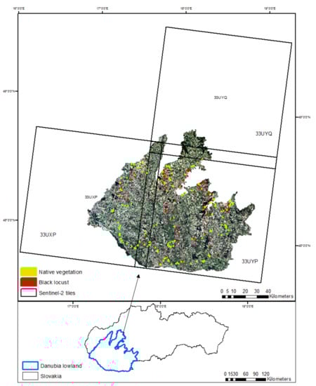
Figure 1.
Study area and distribution of the field-based reference sites (polygons).
2.2. Reference Dataset
A massive field survey was conducted in small woody features [7] across the study area to obtain well distributed samples from both black locusts affected and not affected stands. We adapted and fully applied the publicly available dataset of the Copernicus HRL SWF (https://land.copernicus.eu/pan-european/high-resolution-layers/small-woody-features/small-woody-features-2015, accessed on 10 October 2018) masked by the land cover class 200 (agriculture) of the Copernicus land cover product from 2018 (https://land.copernicus.eu/pan-european/corine-land-cover/clc2018, accessed on 1 Feburary 2019) to properly cover non-forest features in the agricultural landscape. Copernicus HRL SWF product provides harmonized information on linear structures such as hedgerows, scrubs, and tree rows as well as isolated/scattered patches of trees (200 m² ≤ area ≤ 5000 m²) of woody features across the EEA39 countries. The product has been recently validated, reaching a satisfactory accuracy estimation of above 90% of overall accuracy [7]. In particular, small woody features in the Danubian lowland represent combination of remnants of native vegetation (alluvial forests, wetland scrub, thermophilous forests), linear structures (windbreaks, hedgerows, buffer strips at the borders of crop parcels, accompanying vegetation on field roads and river banks), and spontaneous successional vegetation on abandoned or not used sites. In wet places, common willow species (Salix alba, S. fragilis and scrubby willows), poplars (Populus nigra, P. x canescens, P. alba), alder (Alnus glutinosa), bird cherry (Padus avium), and ashes (Fraxinus angustifolia, F. excelsíor) are found. In dry sites grow mostly maples (especially Acer campestre), oaks, elms (especially Ulmus campestre), hornbeam (Carpinus betulus), and scrubs (Prunus spinosa, Rosa canina agg., Crataegus spec. div., Cornus spec. div., Viburnum lantana). We further refer to these types as “native vegetation”.
Black locust stands are widely distributed within non-forest features, though data about their exact occurance are not available as they have not been systematically mapped by any monitoring program. Therefore, a massive field campaign was undertaken in 2018, 2019, and 2021 in order to gather a sufficiently large dataset. The field campaign was conducted during the early spring period (April), allowing easy recognition of the black locust stands since they did not have fully developed leaves compared to surrounding native vegetation in full leaf at that stage (Figure 2). We recorded stands in the field using a rugged field computer (Handheld Algiz) equipped with an integrated U-blox chip capable of achieving spatial precision of 1–3 m. The QGIS software (https://www.qgis.org/en/site/, accessed on 15 January 2020) was used to produce the center points of the homogenous mapped stands. Following the field survey, a manual delineation of black locust and native vegetation stands was conducted using open source QGIS software over 2018 RGB aerial ortophotomaps with a spatial resolution of 25 cm (https://www.geoportal.sk/en/zbgis/orthophotomosaic/1st-cycle-2017-2019/, 5 January 2020). This resulted in the creation of 339 polygons (217 for native—3.44 km2 and 122 for black locust stands—1.36 km2). Finally, reference polygons were randomly sampled for 6000 pixels with a balanced distribution across both classes and then split into training (3000 pixels) and validation (3000 pixels) datasets.
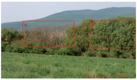
Figure 2.
(A) Black locust in SWF without leaves; (B) Native vegetation in SWF with leaves.
2.3. Satellite Data
The data collected by the MultiSpectral Instrument (MSI) onboard the Sentinel-2A and Sentinel-2B satellites (later referred to as Sentinel-2) were used in the study. In particular, we used Level-2A bottom of atmosphere reflectance products (BOA), which are available in the Google Earth Engine catalogue (ImageCollection ID: COPERNICUS/S2_SR). This product contains BOA reflectances of 13 Sentinel-2 spectral bands and is accompanied by the scene classification (SCL), including quality indicators such as cloud shadow detection, cloud probabilities, and cirrus mask (https://sentinel.esa.int/web/sentinel/technical-guides/sentinel-2-msi/level-2a-processing, 20 November 2021). The BOA reflectances were performed at their native spatial resolutions depending on the spectral characteristics of the respective band. In our analyses, we used Sentinel-2 spectral bands B2, B3, B4, and B8 at native 10 m resolution and bands B5, B6, B7, B8A, B11, and B12 at native 20 m resolution. Three Sentinel-2 tiles were used to fully cover the extent of the study area, namely the 33UYP tile (covering 72.52% of the study area), the 33UXP tile (covering 24.84% of the study area), and the 33UYQ tile (covering 2.64% of the study area).
Only products produced between April and September were used to prevent any quality concerns that might have occurred outside of this time period. As a result, we chose all Sentinel-2 products that were accessible on the GEE platform between 2018 and 2021 (totally 128 datasets).
3. Methodology
The overall approach is described in the workflow diagram (Figure 3) and can be divided into four main stages: (1) Field survey and creation of reference dataset, (2) Spatiotemporal compositing of Sentinel-2 products, (3) Classification and Accuracy Assessment, and (4) Mapping and spatial assessment of black locust distribution.
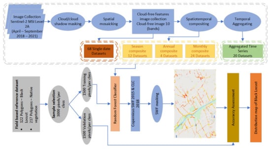
Figure 3.
Workflow diagram.
3.1. Satellite Data Preprocessing
Spatiotemporal compositing followed the obvious steps of so-called pixel-based compositing [41], namely selecting good observations within the compositing period, prioritization, and assignments of target values at the pixel level. We selected the good observations by masking clouds, cloud shadows, and cirrus provided in Level-2A, accompanied by the SCL (scene classification) product. Additionally, a spatial mosaic composed of three Sentinel-2 tiles acquired in a single day was generated, and the proportion of valid observations inside the study area was calculated. If the threshold of 40% cloudfree observation coverage was met, the spatial mosaic would be left for further analysis in the so-called “single-date” classification workflow.
A simple median compositing method were used for producing temporal composite products at different time periods. The median method prioritizes observations closest to the central tendency within a given period and is more resilient against outliers (e.g., unfiltered cloud remnants) than the mean, though is only effective when the majority of selected observations are of good quality. In particular, we computed median values for each spectral band and pixel separately for a given period using GEE’s “imageCollection” function. The same approach has been widely used in many multitemporal classification studies [33,35,42]. Different time intervals were used for compositing, resulting in the creation of annual (six months), seasonal (two months), and monthly composites. In addition, different time series datasets were produced by the temporal aggregation of monthly composites into stacked datasets. Temporal aggregation was performed sequentially within one year, e.g., April 2018 was aggregated with May 2018, followed by adding June 2018, and so on, which resulted in the production of twenty time series datasets (five per each year). All datasets represented inputs for pixel-based classification using the Random Forest algorithm implemented in the GEE platform.
3.2. Random Forest Classifier
The Random Forest Classifier (RF) is widely popular in remote sensing image classification [34,37,43]. The Random Forest algorithm increases the stability and accuracy of classification models [44] and can handle noise in training data and overfitting issues. From the user’s perspective, the main application advantage of RF is that the algorithm needs only two defined parameters: the number of decision trees to run (ntree) and the number of predictors at each decision tree node split (mtry) [45]. Based on the studies of [46,47], we selected 500 ntree, and mtry was set to the default value (equals the number of root mean square of predictive variables).
3.3. Accuracy Assessment
The RF classification models were applied over the study area masked by the SWF HRL [7] and agricultural land cover class 200 (https://land.copernicus.eu/pan-european/corine-land-cover, accessed on 1 February 2019) in order to filter out urban vegetation. Accordingly, classification maps were produced for further accuracy assessments. In addition, class confidence maps were produced that might aid further interpretation of the results. We applied a simple overall accuracy (OA) quantity [48] for quick assessment and comparison of the performance of different classification setups. We used independent validation datasets that were skipped from the training. We assumed no bias in overall accuracy because we employed a balanced validation dataset, e.g., 1500 pixels for black locust stands and 1500 pixels for native stands. The confusion matrix for the best-case classification model was presented, along with the kappa coefficient and producer’s and user’s accuracies [48]. For this reason, the best-case classifications were exported from the GEE for later desktop analyses. A simple majority filter was applied in order to smooth the output map and filter out high-level speckle noise. In addition, a plausibility check was conducted by the visual interpretation of the results followed by field validation of misclassification cases in 2021.
3.4. Spatial Assessment of Black Locust Distribution
The final step represents the spatial assessment of black locust distribution across the study area. The proportion of black locusts within small woody features in polygon representation was produced as an output map accompanied by the histogram depicting its distribution frequency. This was repeated for the 1 × 1 km window in order to better visualize the spatial trend of black locust distribution across the whole area. Finally, we reported spatial statistics on black locust proportional coverage inside 1 km buffer zones around Natura2000 sites to emphasize potential threats of black locust expansion in highly valuable areas. For each cell location in the input value raster, the number of occurrences (frequency) where a raster in the input list has an equal value is counted.
Input rasters
The list of rasters that will be compared against the value raster.
Output raster
The output raster.
For each cell in the output raster, the value represents the number of times that the corresponding cells in the list of rasters are the same as the value raster.
4. Results
Overall, 68 single-date mosaic images were used, with varied classification performances that strongly depend on the quality of the single-date mosaic (Figure 4). Only four single-date mosaics that met less than a 30% cloudiness threshold were available for May, though they performed the best, followed by April and September.
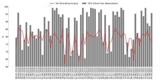
Figure 4.
Overall accuracy and cloud cover of single date images.
In preliminary experiments, it was revealed that the monthly compositing period outscored the seasonal and yearly composing periods (Table 2). Thus, the monthly period seems to be an optimal trade-off between data availability and the persistence of spectrotemporal information, allowing detection of black locust canopies.
Table 2.
Overall accuracy of years, seasons and monthly composites.
Classification models using monthly median composites performed well across years, achieving accuracy estimates of 80 to 86 percent of overall accuracy, demonstrating that the classification models are not much affected by the varied number and quality of observations. Except for the May 2021 monthly composite, which covers 75% of the mapping area, all monthly composites cover the whole mapping area of interest, with an average number of per pixel observations ranging from 3.02 (May 2019) to 7.4 (April 2020). On average, May composites yielded the best results, followed by July and June. Additionally, May composites performed well across years, exhibiting the lowest inter-anual variability of estimated accuracies.
Analysis of feature importance for monthly classification models revealed the high importance of red edge spectral bands (e.g., Sentinel-2 bands 5 and 6) and SWIR spectral bands (e.g., Sentinel-2 bands 11 and 12). This was consistent across years and months, which implies a spectral distinction between black locust canopies and native vegetation mainly in the red edge and SWIR spectral range (Figure 5). Notably, spectral bands B8 and B8A were ranked low in importance across months and years, though comparison of spectral profiles of black locust canopies with those of native vegetation revealed consistent differences in the whole NIR spectral range, including bands B8 and B8A (Figure 6). However, when only four Sentinel-2 spectral bands at their original 10 m resolution were used as classification inputs (data not shown), the NIR band (B8) was ranked as the most important band.
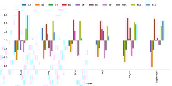
Figure 5.
Standardized variable importance of Sentinel-2 spectral bands of the monthly classification models.
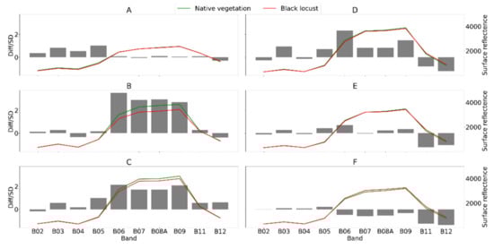
Figure 6.
Spectral profiles (SR*10000) of black locust canopies (red) and native vegetation (green) in monthly composites (A—April; B—May; C—June; D—July; E—August; F—September). Spectral profiles represent means of the 1500 training pixels per each class. Bars represent standardized differences between classes.
The sequential aggregation of monthly composite inputs for developing classification models revealed an apparent characteristic of the RF algorithm that is capable of learning from complex feature spaces. As a result, classification performance gradually improved as the spectrotemporal feature space was expanded through the inclusion of subsequent monthly composites within the vegetation season (Figure 7). This is true unless subsequent monthly composites contain redundant or noisy data, as it was in August and September 2021, when they reached the lowest accuracy in the given year (Table 2). A remarkable increase is apparent even at the beginning of the season after the involvement of the May composites, followed by a slight increase until the end of the season. Finally, high overall accuracy was achieved with balanced producer’s accuracy (PA) and user’s accuracy (UA) for each year’s annual series, with relatively tiny variation across years (Figure 7).
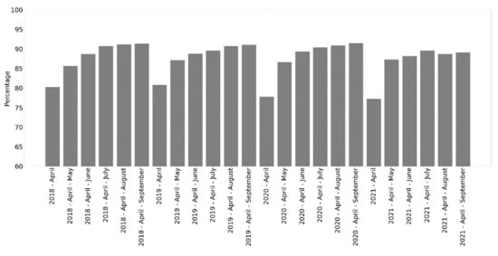
Figure 7.
Overall accuracy of temporally aggregated monthly composites.
As the final models are quite complex, the interpretation of variable importance is not straightforward, though the spectral bands from the SWIR and red edge spectral regions (B11-12, B5-7) were ranked consistently high across the different months (Figure 8).
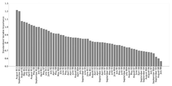
Figure 8.
Variable importance ranked across the different months and years.
Table 3 presents the error matrices of the best-case classification model from 2020. There was no visible pattern in misclassifications, except for mistakenly classifications of black locust stands (comision errors) at the edges of native forest stands when surrounded by arable land. Therefore, a majority filter has been applied in order to smooth fine level speckle noise (Figure 9). The 2020 best-case multitemporal classification model was used to produce the final full-coverage results, including the output classification map (Figure 10), confidence map, and proportion of black locust within SWF in polygon representation (Figure 11). Full resolution maps and vector data are provided in the Supplementary Materials. Within the total 455 square kilometers of small woody features of the Danubian lowland, black locust stands are estimated to cover roughly 56 square kilometers. The distribution of black locust proportions within small woody features is illustrated in Figure 12. It is visible that distribution is skewed towards quasi homogenous stands that represent a substantial proportion of typical monodominant woody features, which might relate to specific historical management, e.g., plantating.
Table 3.
Error matrice of the best-case classification of temporally aggregated monthly composites from 2020.
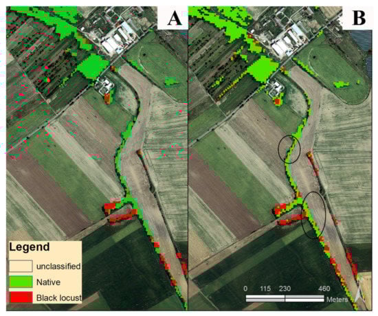
Figure 9.
(A) Classification after majority filter; (B) classification before majority filter—black circles showing typical misclassifications of black locust at the edges of the small woody features.
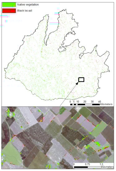
Figure 10.
Distribution map of black locust in the Danubian lowland.
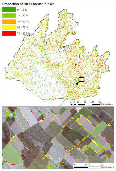
Figure 11.
Map of black locust proportion in small woody features.
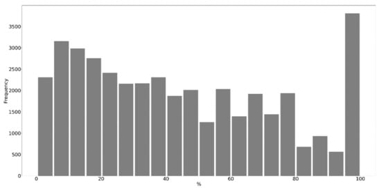
Figure 12.
Distribution of of black locust coverage in small woody features (absences of black locust in SWF, e.g., 0% proportions were omitted for better visualizations; they represent 201,812 cases).
In addition, landscape analysis over a 1 km2 spatial window was conducted for the demonstration of the added value of black locust mapping for spatial assessment of relevant ecosystem services. Though widely dispersed, the specific spatial trends might be visible, e.g., consistently lower proportions of black locust in the southwestern flat Danubian lowlands and lower proportions in alluvial landscapes along the main rivers (Figure 13). Furthermore, the possible threat of black locust invasion to natural ecosystems of high biodiversity values protected in Natura2000 sites was identified. Figure 14 provides the distribution of black locust proportion within 1 km buffer zones of the Natura2000 sites. The diverse proportions might imply different threats to biodiversity and allow the prioritization of subsequent mitigation actions.
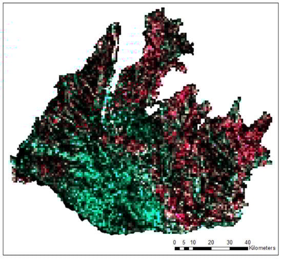
Figure 13.
Proportion of black locust in 1 × 1 km window. RGB composition; red band represents proportion of black locust in SWF in 1 km2; green band represents proportion of native vegetation in SWF in 1 km2; blue band was not used.
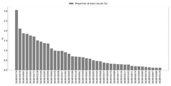
Figure 14.
Proportion of black locust stands within 1 km buffer zone of the Natura2000 sites (SKUEV represent name of the Nature2000 sites (absences of black locust in Natura2000 sites, e.g., 0% proportions were omitted for better visualitzations; they represent 24 cases)).
We also tested the effect of shrinking the training dataset on classification performance from 1500 to 250 training pixels (Table 4). The decrease in OA appeared to be relatively minor until the sample size was reduced substantially from 500 to 250.
Table 4.
Effect of shrinking the training dataset on classification performance.
5. Discussion
The accuracy acceptance levels of spectral classification differ considerably according to specific applications, ranging from 70% [49] to 85% for PA and UA [48].
The direct comparison of accuracy estimates of invasive species detection with other studies is limited for different reasons, such as species-specific distinctive phenology, scale of the studies, classification methods, representativness of the reference datasets, satellite platform and sensors used, etc. Table 1 provides a rough review of accuracy estimates from classification studies using Landsat-like data (e.g., Landsat TM5, ETM+, OLI and Sentinel-2). The accuracy estimates range from 0.7 to 0.9. Our accuracies fell well within this range, signifying good to excellent classification performance, which was surprisingly high in the given conditions, e.g., small scattered patches and thin linear woody features in agricultural landscape.
Somodi et al. [36] predicted the occurence of black locust stands using generalised linear models in a complex agricultural landscape, though with a relatively small extent of approximately 280 km2. Specifically, they used spectral reflectances of Landsat ETM+ separately from May and August as inputs for testing presence/absence models. They documented only moderate success, assessed with an AUC measure ranging from approximately 0.75 to 0.85 (values estimated only from the graphs) according to different reference data used. They stated that the 30 m spatial resolution of Landsat products hampered recognition of black locust stands in a heterogeneous agricultural landscape. They reported that the May image provided better results than that of August, which they explained by the detectable flowering signal of black locust canopies. While May appears to be important in our study as well, we demonstrated that other periods contribute to the classification model’s explanatory power, resulting in significantly improved black locust classification performance when the entire season is considered.
Karasiak [37] used multitemporal classification of forest vegetation based on 11 Sentinel-2 images across the 2016 vegetation season. They achieved very good accuracy estimates for the black locust forest type, reaching F1 scores above 0.9. However, they performed the classification tests on a relatively small study area (approx. 20 × 20 km) and used only homogenous forest stands for training. In addition, ref. [37] identified a slight advancement in the inclusion of the 10 Sentinel spectral bands (F1 score of 0.95) versus the use of only 4 VNIR bands at higher resolution (F1 score of 0.92). Obviously, Sentinel-2 spectral bands at 20 m spatial resolution could be too coarse for mapping highly fragmented SWF alone. On the other hand, utilizing all available spectral information by including Sentinel-2 bands at a spatial resolution of 20m may improve classification performance [50], as was the case also in our study. The use of publicly available high-resolution layers from EEA (European Environment Agency) that utilize VHR images does indeed necessitate subsequent good classification performance by masking nonforest vegetation. In such circumstances, it seems that even the spectral information from the bands originally at 20 m GSD would effectively aid in the exploration of the complex spectrotemporal feature space of highly fragmented small woody features. In any case, post classification adjustment, e.g., majority filtering, would enhance the final product, as commision errors of black locust stands at the edges of SWF were quite obvious (Figure 9). Typical misclassifications occurred at the forest edges when brighter soils next to the native forest stands affected the spectral information of mixed pixels, resulting in erroneous assignment to the black locust class. Similar cases were also reported by [36], where soil brightness was often confused by the black locust flowering signal.
Wang et al. [51] used a spectral index and a supervised maximum likehood algorithm that utilized Landsat SWIR bands to classify black locust stands in the range of 0.71 to 0.96 accuracy. They demonstrated the high spectral separability of black locust stands in Landsat SWIR bands, e.g., TM5 and TM7, based on a better performance compared to the standard NDVI index in several watersheds of the Chinese Loess Plateau. In our study, we also identified the high importance of SWIR bands together with the red edge bands in both monotemporal (Figure 5) and multitemporal (Figure 8) settings. The high importance of red edge spectral bands was widely documented in other vegetation studies [50], which proves the added value of the relatively dense spectral information of the red edge region for revealing the complex spectral responses of different vegetation types. We assume that it is mainly the consistently lower reflectance of black locust canopies in the red edge and near infrared region (Figure 6) that drives the specific spectral response of black locust canopies from May to August. The spectral reflectance in the near infrared spectral region is highly complex and driven mainly by structural properties at the leaf, stem, and canopy scale [52], so we assume that the black locust canopies exhibit specific structural properties that drive their distinctive spectral characteristics in the NIR range. In addition, lower canopy water content that might cause lower reflectances in SWIR B11 and B12 bands (Figure 6) which might reflect drier site conditions occupied by the black locust stands. In fact, remnants of wetland habitats and alluvial forests within the flat Danubian depression in the southwestern part of the study region represent the area with the lowest coverage of black locust stands (Figure 10 and Figure 13). The high importance of the blue band in May might relate to the flowering of black locust stands, though this conclusion remains speculative because we did not perform field validation in that period. Somodi et al. [36] proved May to be the optimal period for distinguishing black locust stands, though the spatiotemporal variability of flowering signals in Central Europe might be great [53].
Meng et al. [38] classified four dominant tree species in the Mount Tai forested landscape for two time periods separately, reaching an overall accuracy of 76% in 2000 and 77% in 2016. They used a multitemporal classification approach by using four Landsat 7 ETM+ images per year (March, July, September, and November) as inputs to the RF classification algorithm. Though they did not discuss the class-specific accuracy estimates of black locust stands, they did document the expansion of the black locust across the forested landscape by 3.6% from 2000 to 2016.
In any case, all of the research discussed above was conducted in rather small areas, which may pose an issue of overfitting. In our study, we tried to deliver a full coverage mapping product for a substantially larger extent, e.g., 9820 km2, based on a relatively massive field-based reference dataset, which might not be feasible for operational monitoring elsewhere. As a response, we investigated the effect of shrinking the training dataset on classification performance, which resulted in unexpectedly acceptable accuracy up to 250 training pixels (Table 4). We think that this is a manageable number of reference datasets in order to replicate the mapping approach elsewhere. In any case, in order to apply the mapping of black locust at a substantially broader scale (e.g., national) where different landscapes and phenology of black locust are expected, intelligent sampling through active learning [54] would be applied in order to ensure effective transferability of the models in spatial dimension [55]. Moreover, when change assessment of expansive black locust canopies is the prime interest [38], the transferability of models on a temporal scale by using different domain adaptation strategies would be applicable [56]. Testing effective strategies of model transferability at a spatiotemporal scale requires future research in order to aid black locust monitoring in wider regions.
As has been frequently described, the RF algorithm appeared to be robust, capable of learning efficiently from nearly any spectrotemporal feature space. Obviously, the more informative the spectrotemporal feature space is (e.g., dense time series vs. single month composite), the better the performance of the classification model. Similar findings are frequently reported for a variety of classification and modelling tasks [34]. Evangelista et al. [21] compared monotemporal with multitemporal approaches for detection of invasive Tamarisk shrubs using six Landsat 7 ETM+ satellite scenes at different times of the growing seasons, e.g., April, May, June, August, September, and October, as inputs to the Maxent model. They documented the improved performance of the full multitemporal model that used all 72 variables compared to single-scene models. Generally, the results from the single-scene analyses improved toward the latter part of the growing season and into the fall months, when most native plants go into dormancy. We also documented the substantial enhancement of multitemporal models compared to single-month models across all years, which might have documented the robustness of the RF algorithm. Furthermore, when single-month classifications are considered, May and April models outperformed those from the seasonal peak. In many classification tasks, however, annual best pixel strategies often select summer images, ensuring both image quality and the greenest pixels available, assuming maximum contrast between land cover classes exists during the peak vegetation season [57]. On the other hand, when mapping is focused only on vegetated surfaces, greenness and vigour signals might be saturated during seasonal peaks, which might be the reason for the relatively low classification power of summer models (Table 2). When special interest is taken in species with contrasting phenologies, specific periods in early spring or late autumn could be advantageous. Anyway, due to sun viewing geometry, image quality is frequently compromised at these times due to extended shadow casting during the morning acquisition time. Therefore, there is an obvious trade-off between image quality and the optimal selection of phenologically distinct periods. In our case, April and September composites appear to be beneficial in multitemporal settings (Figure 7), however, single month models of the September and April composites performed slightly worse than summer months (Table 2). Cloudiness appeared to be a significant concern in May, but spatiotemporal compositing effectively handled this issue.
The higher proportion of black locusts in SWF mimics the distribution of areas with the highest occurrence of Robinia pseudoacacia in Central European countries [3]. In particular, these are mainly uplands and river terraces in the southeastern part of the greater Danubian lowlands where black locust stands predominate in SWF. On the other hand, Danubian flat depressions with remnants of natural wetland vegetation and alluvial forests in the southwestern part of the greater Danubian lowlands represent an area with the minimal occurence of black locust stands. The output of this study represents the first distribution map of black locust stands in the agricultural landscape on a regional scale and will serve as the basis for a potential large-scale assessment of different ecosystem services. Additionally, a distribution map of black locust stands throughout Natura2000 areas might aid in the development of appropriate nature conservation management actions to mitigate possible risks to biodiversity posed by black locust expansion. It is important to notice here that this kind of information at such a detailed scale is missing in Slovakia, and black locust stands are only monitored in forested landscapes via demanding field-based inventories conducted by the national forest service.
The important finding from the user perspective is that monthly median composites have not been much affected by the quality of observations. In particular, the performance was quite good in months where a small number of clear observations existed, e.g., May, and also in months where more observations existed, e.g., July. We demonstrated that the RF algorithms can effectively handle both situations, and the monthly composite series seems to be optimal for exploration of spectrotemporal feature space in SWF. The Google Earth Engine certainly accelerates large-scale processing of the publicly available RS data. It is unique in the field as an integrated platform designed to empower not only traditional remote sensing scientists, but also a much wider audience that lacks the technical capacity needed to utilize traditional supercomputers or large-scale commodity cloud computing resources. However, some essential programming skills, such as basic Python or Java script programming skills, may prevent this platform from being considered user-friendly. In any case, given the multitemporal classification approach used in our study, we can anticipate an increase in the value of the GEE platform as available Sentinel-2 time series are sequentially expanded.
In this study, we used simple compositing methods motivated by their straightforward application. Unlike precise harmonisation of input data by spatiotemporal coherent composing [58], we applied a data-driven approach based on the massive classification of all inputs with a relatively low level of spatiotemporal coherence followed by their tailored aggregation. However, because the data-driven approach used here possesses apparent limits in terms of transferability across space and time, future research should focus on a more in-depth exploration of the possible added value of recently discovered advanced compositing algorithms that maintain spatiotemporal coherence in input data. This could have prospects for later development of more robust and transferable models in domains with scarce reference data and high interannual dynamics, e.g., rapid invasive species expansion.
6. Conclusions
In this study, we demonstrated that using the spatiotemporal composite RS products’ classification of black locust stands within small woody features in a wide agricultural landscape is possible. The main reason for this could be related to the non-native vegetation’s distinctive spectral response. In particular, distinction was evident across all seasons, being the highest in the beginning of the vegetation season, which might be driven by the different phenology of black locust, e.g., later onset of greeness and specific flowering. More detailed research on specific spectral characteristics of non-native black locust canopies is open for further research, mainly with the prospects of the recent and upcoming space-borne spectral imaging missions such as PRISMA, EnMAP, or CHIME. The spatial detail of detectable black locust stands was surprisingly high. The support of the Copernicus HRL spatial mask that reduced the complex spectral space of the agricultural landscape might have been critical. Further studies should be conducted in this respect to apply the whole processing chain across the entire agricultural landscape in order to replicate the approach in regions where Copernicus HRL is not available. Even though black locusts are supposed to be widely distributed in Central Europe, landscape analysis revealed that the spatial trends can be seen at a regional level. This could be because of historical management (e.g., planting) or environmental constraints of the specific site conditions. Further research into the detailed knowledge of the driving factors behind the spatial pattern of black locust distribution at a regional scale is needed. Finally, maps of broad-area black locust distribution at high spatial resolution may be used to support both the spatial assessment of ecosystem services and the mitigation of potential negative effects on biodiversity in agricultural landscapes.
Supplementary Materials
The following supporting information can be downloaded at: https://www.mdpi.com/article/10.3390/rs14040971/s1. The material represents mainly raw data, including those for the training and validation, in order to facilitate their usage from both methodological (e.g., different classification algorithms and settings) and thematic (e.g., ecosystem assessments, etc.) aspects. File S1: Confidence_of_BL.tif—Raster file contains confidence map of black locust in SWF; File S2: Danubian_lowland.shp—Study area ROI (See Figure 1 and Section 2.1); File S3: Distribution_of_BL.tif—Raster file contains the distribution map of black locust from multitemporal classification model (see Figure 10); File S4: Proportion_of_BL_in_SWF.shp—Dataset of black locust proportion in SWF, the attribute table contains the following fields: “ID” represents ID of polygon; field “Area_m2” represents area in square meters of black locust; field “AG_pro” represents percentual proportion of black locust in the SWF polygon (see Figure 11); File S5: Reference_data.shp—Reference dataset, the attribute table contains the following fields “Class” where is information about class assignment to the black locust or native vegetation; field “Trieda” represent the same infomation but in integer format: 1—black locust and 2—native vegetation; field “Area” represent size of the SWF polygon in square meters; field “Perim” represent perimeter of the SWF polygons in square meters; field ”ShapIndex” represents the Shape Index (see Figure 1 and Section 2.2). File S6: Natura2000_Proportion_BL.csv—File contains proportion of black locust stands within 1 km buffer zone of the Natura2000 sites—column “KOD” represents Site Name; column “Prop_AGAT_percent” represents percentual proportion of black locust within 1 × 1 km2 buffer zone of the Natura2000 site (See Figure 14).
Author Contributions
Conceptualization: T.R. and A.H.; methodology: T.R. and A.H.; software: T.R. and A.H.; validation: T.R. and A.H.; data collection: T.R., A.H., K.G. and H.H.; visualization: T.R.; writing—original draft preparation: T.R. and A.H.; writing—review and editing: T.R., A.H. and Ľ.H. All authors have read and agreed to the published version of the manuscript.
Funding
This research was supported by the Integrated Infrastructure Operational Programme funded by the ERDF, project ITMS2014+ 313011W580, “Scientific support of climate change adaptation in agriculture and mitigation of soil degradation” (80%), by the Slovak Research and Development Agency (APVV), project No. APVV-17-0377 “Assessment of recent changes and trends in agricultural landscape of Slovakia”, and by the Slovak Scientific Grant Agency VEGA 2/0018/19 “Ecological Analyses of Landscape acculturation in Slovakia since Early Prehistory until Today”.
Data Availability Statement
The reference dataset is attached as Supplementary Material available at https://figshare.com/articles/dataset/Supplements_rar/19126682, accessed on 9 February 2022; Corin Land Cover 2018 is available at the Copernicus Services website https://land.copernicus.eu/pan-european/corine-land-cover/clc2018, accessed on 9 February 2022; Small-woody features HRL 2015 dataset is available at the Copernicus Services website https://land.copernicus.eu/pan-european/high-resolution-layers/small-woody-features/small-woody-features-2015, accessed on 9 February 2022; The Aerial ortophotomaps of Slovakia with a spatial resolution of 25 cm are available at https://www.geoportal.sk/en/zbgis/orthophotomosaic/1st-cycle-2017-2019/, accessed on 9 February 2022.
Acknowledgments
We thank the three anonymous reviewers for their valuable comments.
Conflicts of Interest
The authors declare no conflict of interest.
References
- Richardson, D.M.; Rejmánek, M. Trees and Shrubs as Invasive Alien Species-a Global Review: Global Review of Invasive Trees & Shrubs. Divers. Distrib. 2011, 17, 788–809. [Google Scholar] [CrossRef]
- Cierjacks, A.; Kowarik, I.; Joshi, J.; Hempel, S.; Ristow, M.; von der Lippe, M.; Weber, E. Biological Flora of the British Isles: Robinia pseudoacacia. J. Ecol. 2013, 101, 1623–1640. [Google Scholar] [CrossRef]
- Vítková, M.; Müllerová, J.; Sádlo, J.; Pergl, J.; Pyšek, P. Black Locust (Robinia Pseudoacacia) Beloved and Despised: A Story of an Invasive Tree in Central Europe. For. Ecol. Manag. 2017, 384, 287–302. [Google Scholar] [CrossRef]
- Rice, S.K.; Westerman, B.; Federici, R. Impacts of the Exotic, Nitrogen-Fixing Black Locust (Robinia Pseudoacacia) on Nitrogen-Cycling in a Pine–Oak Ecosystem. Plant Ecol. Former. Veg. 2004, 174, 97–107. [Google Scholar] [CrossRef]
- Skuhravá, M.; Skuhravý, V.; Csóka, G. The Invasive Spread of the Gall Midge Obolodiplosis Robiniae in Europe. Cecidology-Leyburn 2007, 22, 2–84. [Google Scholar]
- Buhl, P.N.; Duso, C. Platygaster robiniae n. Sp. (Hymenoptera: Platygastridae) Parasitoid of Obolodiplosis robiniae (Diptera: Cecidomyiidae) in Europe. Ann. Entomol. Soc. Am. 2008, 101, 297–300. [Google Scholar] [CrossRef] [Green Version]
- Langanke, T.; Desclee, B.; Faucquer, L.; Moser, L.; Schleicher, C.; Schnelle, M. Copernicus Land Monitoring Service—High Resolution Layer Small Woody Features—2015; European Environment Agency: København, Denmark, 2012. [Google Scholar]
- Rega, C.; Bartual, A.M.; Bocci, G.; Sutter, L.; Albrecht, M.; Moonen, A.-C.; Jeanneret, P.; van der Werf, W.; Pfister, S.C.; Holland, J.M.; et al. A Pan-European Model of Landscape Potential to Support Natural Pest Control Services. Ecol. Indic. 2018, 90, 653–664. [Google Scholar] [CrossRef]
- Joshi, C.; de Leeuw, J.; van Duren, I.C. Remote Sensing and Gis Applications for Mapping and Spatial Modelling of Invasive Species. In Proceedings of the ISPRS 2004: The XXth ISPRS Congress: Geo-Imagery Bridging Continents, Istanbul, Turkey, 12–23 July 2004. [Google Scholar]
- Huang, C.; Asner, G. Applications of Remote Sensing to Alien Invasive Plant Studies. Sensors 2009, 9, 4869–4889. [Google Scholar] [CrossRef] [PubMed] [Green Version]
- Bradley, B.A. Remote Detection of Invasive Plants: A Review of Spectral, Textural and Phenological Approaches. Biol. Invasions 2014, 16, 1411–1425. [Google Scholar] [CrossRef]
- He, K.S.; Rocchini, D.; Neteler, M.; Nagendra, H. Benefits of Hyperspectral Remote Sensing for Tracking Plant Invasions: Plant Invasion and Hyperspectral Remote Sensing. Divers. Distrib. 2011, 17, 381–392. [Google Scholar] [CrossRef]
- Ramsey, E., III; Rangoonwala, A.; Nelson, G.; Ehrlich, R. Mapping the Invasive Species, Chinese Tallow, with EO1 Satellite Hyperion Hyperspectral Image Data and Relating Tallow Occurrences to a Classified Landsat Thematic Mapper Land Cover Map. Int. J. Remote Sens. 2005, 26, 1637–1657. [Google Scholar] [CrossRef]
- Somers, B.; Asner, G.P. Hyperspectral Time Series Analysis of Native and Invasive Species in Hawaiian Rainforests. Remote Sens. 2012, 4, 2510–2529. [Google Scholar] [CrossRef] [Green Version]
- Becker, R.H.; Zmijewski, K.A.; Crail, T. Seeing the Forest for the Invasives: Mapping Buckthorn in the Oak Openings. Biol. Invasions 2013, 15, 315–326. [Google Scholar] [CrossRef]
- Fuller, D.O. Remote Detection of Invasive Melaleuca Trees (Melaleuca Quinquenervia) in South Florida with Multispectral IKONOS Imagery. Int. J. Remote Sens. 2005, 26, 1057–1063. [Google Scholar] [CrossRef]
- Lantz, N.J.; Wang, J. Object-Based Classification of Worldview-2 Imagery for Mapping Invasive Common Reed, Phragmites Australis. Can. J. Remote Sens. 2013, 14, 328–340. [Google Scholar] [CrossRef]
- Gil, A.; Lobo, A.; Abadi, M.; Silva, L.; Calado, H. Mapping Invasive Woody Plants in Azores Protected Areas by Using Very High-Resolution Multispectral Imagery. Eur. J. Remote Sens. 2013, 46, 289–304. [Google Scholar] [CrossRef] [Green Version]
- Müllerová, J.; Pergl, J.; Pyšek, P. Remote Sensing as a Tool for Monitoring Plant Invasions: Testing the Effects of Data Resolution and Image Classification Approach on the Detection of a Model Plant Species Heracleum Mantegazzianum (Giant Hogweed). Int. J. Appl. Earth Obs. Geoinf. 2013, 25, 55–65. [Google Scholar] [CrossRef]
- Peterson, E.B. Estimating Cover of an Invasive Grass (Bromus Tectorum) Using Tobit Regression and Phenology Derived from Two Dates of Landsat ETM+ Data. Int. J. Remote Sens. 2005, 26, 2491–2507. [Google Scholar] [CrossRef]
- Evangelista, P.; Stohlgren, T.; Morisette, J.; Kumar, S. Mapping Invasive Tamarisk (Tamarix): A Comparison of Single-Scene and Time-Series Analyses of Remotely Sensed Data. Remote Sens. 2009, 1, 519–533. [Google Scholar] [CrossRef] [Green Version]
- Wilfong, B.N.; Gorchov, D.L.; Henry, M.C. Detecting an Invasive Shrub in Deciduous Forest Understories Using Remote Sensing. Weed Sci. 2009, 57, 512–520. [Google Scholar] [CrossRef]
- Olsson, A.D.; van Leeuwen, W.J.D.; Marsh, S.E. Feasibility of Invasive Grass Detection in a Desertscrub Community Using Hyperspectral Field Measurements and Landsat TM Imagery. Remote Sens. 2011, 3, 2283–2304. [Google Scholar] [CrossRef] [Green Version]
- Gavier-Pizarro, G.I.; Kuemmerle, T.; Hoyos, L.E.; Stewart, S.I.; Huebner, C.D.; Keuler, N.S.; Radeloff, V.C. Monitoring the Invasion of an Exotic Tree (Ligustrum lucidum) from 1983 to 2006 with Landsat TM/ETM+ Satellite Data and Support Vector Machines in Córdoba, Argentina. Remote Sens. Environ. 2012, 122, 134–145. [Google Scholar] [CrossRef] [Green Version]
- Ai, J.; Gao, W.; Gao, Z.; Shi, R.; Zhang, C.; Liu, C. Integrating Pan-Sharpening and Classifier Ensemble Techniques to Map an Invasive Plant (Spartina alterniflora) in an Estuarine Wetland Using Landsat 8 Imagery. J. Appl. Remote Sens. 2016, 10, 026001. [Google Scholar] [CrossRef]
- Hauglin, M.; Ørka, H. Discriminating between Native Norway Spruce and Invasive Sitka Spruce—A Comparison of Multitemporal Landsat 8 Imagery, Aerial Images and Airborne Laser Scanner Data. Remote Sens. 2016, 8, 363. [Google Scholar] [CrossRef] [Green Version]
- Forster, M.; Schmidt, T.; Wolf, R.; Kleinschmit, B.; Fassnacht, F.E.; Cabezas, J.; Kattenborn, T. Detecting the Spread of Invasive Species in Central Chile with a Sentinel-2 Time-Series. In Proceedings of the 2017 9th International Workshop on the Analysis of Multitemporal Remote Sensing Images (MultiTemp), Brugge, Belgium, 27–29 June 2017; IEEE: Piscataway, NJ, USA, 2017; pp. 1–4. [Google Scholar] [CrossRef]
- de Sá, N.C.; Castro, P.; Carvalho, S.; Marchante, E.; López-Núñez, F.A.; Marchante, H. Mapping the Flowering of an Invasive Plant Using Unmanned Aerial Vehicles: Is There Potential for Biocontrol Monitoring? Front. Plant Sci. 2018, 9, 293. [Google Scholar] [CrossRef] [PubMed] [Green Version]
- Kganyago, M.; Odindi, J.; Adjorlolo, C.; Mhangara, P. Evaluating the Capability of Landsat 8 OLI and SPOT 6 for Discriminating Invasive Alien Species in the African Savanna Landscape. Int. J. Appl. Earth Obs. Geoinf. 2018, 67, 10–19. [Google Scholar] [CrossRef]
- Resasco, J.; Hale, A.N.; Henry, M.C.; Gorchov, D.L. Detecting an Invasive Shrub in a Deciduous Forest Understory Using Late-fall Landsat Sensor Imagery. Int. J. Remote Sens. 2007, 28, 3739–3745. [Google Scholar] [CrossRef]
- He, M.; Zhao, B.; Ouyang, Z.; Yan, Y.; Li, B. Linear Spectral Mixture Analysis of Landsat TM Data for Monitoring Invasive Exotic Plants in Estuarine Wetlands. Int. J. Remote Sens. 2010, 31, 4319–4333. [Google Scholar] [CrossRef]
- Villarreal, M.; Soulard, C.; Waller, E. Landsat Time Series Assessment of Invasive Annual Grasses Following Energy Development. Remote Sens. 2019, 11, 2553. [Google Scholar] [CrossRef] [Green Version]
- Xie, S.; Liu, L.; Zhang, X.; Yang, J.; Chen, X.; Gao, Y. Automatic Land-Cover Mapping Using Landsat Time-Series Data Based on Google Earth Engine. Remote Sens. 2019, 11, 3023. [Google Scholar] [CrossRef] [Green Version]
- Phan, T.N.; Kuch, V.; Lehnert, L.W. Land Cover Classification Using Google Earth Engine and Random Forest Classifier—The Role of Image Composition. Remote Sens. 2020, 12, 2411. [Google Scholar] [CrossRef]
- Jia, M.; Mao, D.; Wang, Z.; Ren, C.; Zhu, Q.; Li, X.; Zhang, Y. Tracking Long-Term Floodplain Wetland Changes: A Case Study in the China Side of the Amur River Basin. Int. J. Appl. Earth Obs. Geoinf. 2020, 92, 102185. [Google Scholar] [CrossRef]
- Somodi, I.; Čarni, A.; Ribeiro, D.; Podobnikar, T. Recognition of the Invasive Species Robinia Pseudacacia from Combined Remote Sensing and GIS Sources. Biol. Conserv. 2012, 150, 59–67. [Google Scholar] [CrossRef]
- Karasiak, N.; Sheeren, D.; Fauvel, M.; Willm, J.; Dejoux, J.-F.; Monteil, C. Mapping Tree Species of Forests in Southwest France Using Sentinel-2 Image Time Series. In Proceedings of the 2017 9th International Workshop on the Analysis of Multitemporal Remote Sensing Images (MultiTemp), Brugge, Belgium, 27–29 June 2017; IEEE: Piscataway, NJ, USA, 2017; pp. 1–4. [Google Scholar] [CrossRef]
- Meng, Y.; Cao, B.; Mao, P.; Dong, C.; Cao, X.; Qi, L.; Wang, M.; Wu, Y. Tree Species Distribution Change Study in Mount Tai Based on Landsat Remote Sensing Image Data. Forests 2020, 11, 130. [Google Scholar] [CrossRef] [Green Version]
- Miklós, L.; Izakovičová, Z. Atlas of Representative Geoecosystems of Slovakia; Slovak Academy of Sciences, Ministry of Environment and Ministry of Education of the Slovak Republik: Bratislava, Slovakia, 2006; pp. 95–123. ISBN 80-969272-4-8. [Google Scholar]
- Lapin, M.; Faako, P.; Melo, M.; Stastny, P.; Tomlain, J. Climatic Regions; 1:1,000,000; 27. Klimaticke Oblasti; 1:1,000,000; Ministry of Environment of the Slovak Republic Bratislava: Bratislava, Slovakia, 2002; ISBN 80-88833-27-2. [Google Scholar]
- Griffiths, P.; van der Linden, S.; Kuemmerle, T.; Hostert, P. A Pixel-Based Landsat Compositing Algorithm for Large Area Land Cover Mapping. IEEE J. Sel. Top. Appl. Earth Obs. Remote Sens. 2013, 6, 2088–2101. [Google Scholar] [CrossRef]
- Carrasco, L.; O’Neil, A.; Morton, R.; Rowland, C. Evaluating Combinations of Temporally Aggregated Sentinel-1, Sentinel-2 and Landsat 8 for Land Cover Mapping with Google Earth Engine. Remote Sens. 2019, 11, 288. [Google Scholar] [CrossRef] [Green Version]
- Huang, H.; Chen, Y.; Clinton, N.; Wang, J.; Wang, X.; Liu, C.; Gong, P.; Yang, J.; Bai, Y.; Zheng, Y.; et al. Mapping Major Land Cover Dynamics in Beijing Using All Landsat Images in Google Earth Engine. Remote Sens. Environ. 2017, 202, 166–176. [Google Scholar] [CrossRef]
- Cutler, D.R.; Edwards, T.C.; Beard, K.H.; Cutler, A.; Hess, K.T.; Gibson, J.; Lawler, J.J. Random forests for classification in ecology. Ecology 2007, 88, 2783–2792. [Google Scholar] [CrossRef]
- Breiman, L. Random Forests. Mach. Learn. 2001, 45, 5–32. [Google Scholar] [CrossRef] [Green Version]
- Zhao, Q.; Yu, S.; Zhao, F.; Tian, L.; Zhao, Z. Comparison of Machine Learning Algorithms for Forest Parameter Estimations and Application for Forest Quality Assessments. For. Ecol. Manag. 2019, 434, 224–234. [Google Scholar] [CrossRef]
- Wang, H.; Zhong, Y.; Pu, R.; Zhao, Y.; Song, Y.; Li, G. Dynamic Analysis of Robinia pseudoacacia Forest Health Levels from 1995 to 2013 in the Yellow River Delta, China Using Multitemporal Landsat Imagery. Int. J. Remote Sens. 2018, 39, 4232–4253. [Google Scholar] [CrossRef]
- Foody, G.M. Status of Land Cover Classification Accuracy Assessment. Remote Sens. Environ. 2002, 80, 185–201. [Google Scholar] [CrossRef]
- Pringle, R.M.; Syfert, M.; Webb, J.K.; Shine, R. Quantifying Historical Changes in Habitat Availability for Endangered Species: Use of Pixel- and Object-Based Remote Sensing. J. Appl. Ecol. 2009, 46, 544–553. [Google Scholar] [CrossRef]
- Immitzer, M.; Vuolo, F.; Atzberger, C. First Experience with Sentinel-2 Data for Crop and Tree Species Classifications in Central Europe. Remote Sens. 2016, 8, 166. [Google Scholar] [CrossRef]
- Wang, H.; Pu, R.; Zhu, Q.; Ren, L.; Zhang, Z. Mapping Health Levels of Robinia pseudoacacia Forests in the Yellow River Delta, China, Using IKONOS and Landsat 8 OLI Imagery. Int. J. Remote Sens. 2015, 36, 1114–1135. [Google Scholar] [CrossRef]
- Ollinger, S.V. Sources of Variability in Canopy Reflectance and the Convergent Properties of Plants. New Phytol. 2011, 189, 375–394. [Google Scholar] [CrossRef] [PubMed]
- Müllerová, J.; Brůna, J.; Bartaloš, T.; Dvořák, P.; Vítková, M.; Pyšek, P. Timing Is Important: Unmanned Aircraft vs. Satellite Imagery in Plant Invasion Monitoring. Front. Plant Sci. 2017, 8, 887. [Google Scholar] [CrossRef] [PubMed] [Green Version]
- Berger, K.; Caicedo, J.P.R.; Martino, L.; Wocher, M.; Hank, T.; Verrelst, J. A Survey of Active Learning for Quantifying Vegetation Traits from Terrestrial Earth Observation Data. Remote Sens. 2021, 13, 287. [Google Scholar] [CrossRef]
- Hamrouni, Y.; Paillassa, E.; Chéret, V.; Monteil, C.; Sheeren, D. From Local to Global: A Transfer Learning-Based Approach for Mapping Poplar Plantations at National Scale Using Sentinel-2. ISPRS J. Photogramm. Remote Sens. 2021, 171, 76–100. [Google Scholar] [CrossRef]
- Demir, B.; Bovolo, F.; Bruzzone, L. Updating Land-Cover Maps by Classification of Image Time Series: A Novel Change-Detection-Driven Transfer Learning Approach. IEEE Trans. Geosci. Remote Sens. 2013, 51, 300–312. [Google Scholar] [CrossRef]
- Cuneo, P.; Jacobson, C.R.; Leishman, M.R. Landscape-Scale Detection and Mapping of Invasive African Olive (Olea Europaea L. Ssp. Cuspidata Wall Ex G. Don Ciferri) in SW Sydney, Australia Using Satellite Remote Sensing. Appl. Veg. Sci. 2009, 12, 145–154. [Google Scholar] [CrossRef]
- Frantz, D.; Röder, A.; Stellmes, M.; Hill, J. Phenology-Adaptive Pixel-Based Compositing Using Optical Earth Observation Imagery. Remote Sens. Environ. 2017, 190, 331–347. [Google Scholar] [CrossRef] [Green Version]
Publisher’s Note: MDPI stays neutral with regard to jurisdictional claims in published maps and institutional affiliations. |
© 2022 by the authors. Licensee MDPI, Basel, Switzerland. This article is an open access article distributed under the terms and conditions of the Creative Commons Attribution (CC BY) license (https://creativecommons.org/licenses/by/4.0/).