Abstract
Waterlogging crop disasters are caused by continuous and excessive soil water in the upper layer of soil. In order to enable waterlogging monitoring, it is important to collect continuous and accurate soil moisture data. The distributed hydrology soil vegetation model (DHSVM) is selected as the basic hydrological model for soil moisture estimation and winter-wheat waterlogging monitoring. To handle the error accumulation of the DHSVM and the poor continuity of remote sensing (RS) inversion data, an agro-hydrological model that assimilates RS inversion data into the DHSVM is used for winter-wheat waterlogging monitoring. The soil moisture content maps retrieved from satellite images are assimilated into the DHSVM by the successive correction method. Moreover, in order to reduce the modeling error accumulation, monthly and real-time RS inversion maps that truly reflect local soil moisture distributions are regularly assimilated into the agro-hydrological modeling process each month. The results show that the root mean square errors (RMSEs) of the simulated soil moisture value at two in situ experiment points were 0.02077 and 0.02383, respectively, which were 9.96% and 12.02% of the measured value. From the accurate and continuous soil moisture results based on the agro-hydrological assimilation model, the waterlogging-damaged ratio and grade distribution information for winter-wheat waterlogging were extracted. The results indicate that there were almost no high-damaged-ratio and severe waterlogging damage areas in Lixin County, which was consistent with the local field investigation.
1. Introduction
Crop waterlogging disasters, which affect crop growth and reduce grain yield [1,2], are caused by excessive water in the crop root zone that disturbs the equilibrium between water and air. The main factors that influence the occurrence of waterlogging are precipitation, topographic conditions, soil physical properties, farming methods, and drainage and irrigation conditions [3]. According to statistics, waterlogging reduces winter-wheat production by more than 50–70%, and long-term waterlogging of farmland aggravates soil salinization [4]. Waterlogging has become an important limiting factor of agricultural development and jeopardizes national food security. Therefore, accurate assessment and real-time analysis of waterlogging are critical for regional waterlogging prevention, which can lay a solid foundation for improving agricultural production capacity. The existing monitoring methods of waterlogging either consider redundant factors, resulting in excessive investment in human and material resources, or adopt insufficient influencing factors, resulting in low accuracy of waterlogging monitoring.
There are three main ways to study waterlogging damage. One traditional research method is to construct a waterlogging damage classification model by sorting and analyzing historical point observation data. However, this method needs a lot of manpower and material resources to obtain data in situ. Its research results are only representative in the small area near the observation point [5]. Another method is to retrieve soil moisture by remote sensing (RS) according to the correlation between the backscattering coefficient and soil water content [6,7,8]. The RS inversion soil moisture data are then used to monitor waterlogging damage [9]. Liu et al. mapped waterlogging damage on winter wheat at the parcel level using high-spatial-resolution satellite data [10]. Sentinel-1 and Sentinel-2 data were also used to estimate soil moisture in recent years. Maurya and Singh [11] made an attempt to use Sentinel-1 data to estimate soil moisture by minimizing the effect of other signal contributors. Chatterjee et al. [12] established an empirical model for surface soil moisture using Sentinel-1 data and ancillary data. Montaldo et al. [13] offered a simplified approach for estimating the surface roughness by Sentinel-2 optical observations to assimilate Sentinel-1 observations in a land surface model. The accuracy of remote sensing technology is relatively high for a large area. However, the same area can be observed again only after a revisit cycle, thereby failing to reflect the continuous process of waterlogging [14]. In recent years, hydrological models combined with DEM, vegetation distribution, soil distribution, and meteorological data have been used to simulate farmland moisture movement and waterlogging monitoring [15]. Singh et al. simulated the groundwater level change of farmland with a spatial agro-hydro-salinity model (SAHYSMOD) to monitor waterlogging and salinization [16,17]. Xiong monitored the subsurface waterlogging of summer crops using a distributed hydrology soil vegetation model (DHSVM) [18]. Hydrological models simulate the continuous temporal variation of soil moisture as needed to monitor the continuous process of waterlogging damage. However, the errors in the model gradually accumulate and distort the model results [19].
Various hydrological models have been used to simulate time-continuous soil moisture data at the regional scale, such as the system hydrological European (SHE) model [20], the Xinanjiang model [21], and the DHSVM [22]. Agro-hydrological models included in the hydrological models are built in order to link both agronomical processes with spatially explicit hydrological fluxes [23], such as the distributed agro-hydrological topography nitrogen transfer and transformation (TNT2) [24] model. The transport of soil water and salt in agricultural farmlands is mainly one-dimensional vertical flow, and is described by one-dimensional dynamic agro-hydrological models, such as the soil-water-atmosphere-plant (SWAP) model [25] and Hydrus model [26]. However, the authenticity and reliability of the simulation are not as good as remote sensing reversion or field measurement. It is difficult to truly reflect the surface soil moisture by a single method, regardless of microwave remote sensing, field measurement devices, or model simulations. Effective multisource data fusion or model–data assimilation have been the important means for acquiring accurate and regional data. Delphine et al. [27] assimilated soil moisture ocean salinity (SMOS) soil moisture into the DHSVM model and discussed the impacts on the simulations of the water cycle variables. Xiong et al. [14] extracted the spatial distribution of subsurface waterlogging using an antecedent precipitation index and RS inversion soil moisture data. Zhu [28] and Yang [29] took the Hetao irrigation area and Weigan–Kuqa River Basin as examples to verify the effectiveness of multisource data assimilation. Compared with other methods, the model–data assimilation methods meet the requirements of both the regional scale and time continuity [30,31].
According to the monitoring results of soil moisture and agro-meteorological disasters, waterlogging damage mostly occurs when the soil relative humidity is more than 90% and lasts for many days [3,14,32]. Meanwhile, accurate and time-continuous soil moisture data are provided by assimilating remote sensing observations and model simulations [20,21]. Therefore, in order to monitor the continuous process of regional waterlogging damage, it is necessary to assimilate multi-temporal area observations from remote sensing inversion into a hydrological model with good continuity. In this paper, the soil moisture data obtained by Sentinel-1 image inversion are used as observations and the initial state files in order to drive the DHSVM hydrological model. The soil moisture files with remote sensing inversion are periodically assimilated into the DHSVM model in the simulation process. The data assimilation theory efficiently reduces the uncertainty of the original DHSVM model, and provides an effective method for obtaining the spatiotemporal-continuous distribution information of soil moisture, which is used to monitor waterlogging.
Lixin County in Anhui Province, China, was selected as the study area of waterlogging monitoring. The DHSVM model was used to simulate the hydrological characteristics of the Xifei River watershed including Lixin County. In order to reduce the errors that the uncertainty in model parameters leads to, we conducted parameter optimization steps including sensitivity analysis, calibration, and optimal spatiotemporal resolution selection using the DHSVM model. The remote sensing inversion data of soil moisture were acquired from the Sentinel-1 images based on the water cloud model (WCM) first proposed by Attema and Ulaby [33]. The agro-hydrological assimilation model constructed by assimilating RS inversion data into the DHSVM was used for winter-wheat waterlogging monitoring. The assimilation method for incorporating remote sensing inversion data into the DHSVM is the successive correction method first proposed by Cressman [34]. In order to obtain accurate and time-continuous soil moisture data, the feasibility and improvement effect of the data assimilation model were also discussed. The winter-wheat waterlogging distribution area in Lixin County was finally obtained through the assimilated soil moisture data. The monitoring results support real-time monitoring and effective control of waterlogging damage, contributing to the stable increase of grain production and the safety assurance of national agricultural production.
2. Study Area and Data Acquisition
2.1. Study Area
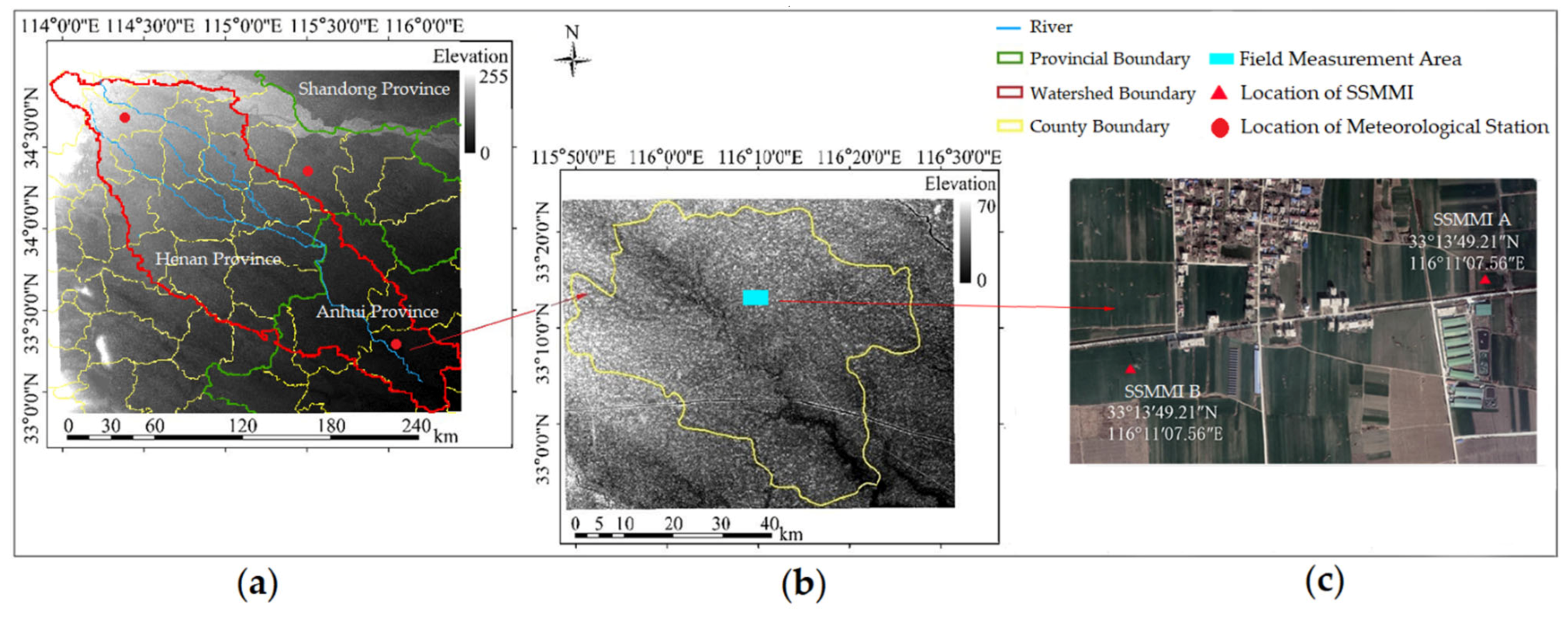
This study aimed to monitor winter-wheat waterlogging in Lixin County. Lixin County has an area of 1950 km2 and is located in the northwest of Anhui Province, China. An area of sandy ginger-black soil accounts for 95.7% of the county’s soil area. Lixin County has a warm, temperate semi-humid monsoon climate, which is rainy in summer and dry in winter. The annual average temperature is 14.7 °C, the annual frost-free period is more than 200 days, and the annual average rainfall is more than 850 mm. The geographical location of Lixin County is shown in Figure 1b. The Xifei River, originating from Taikang County in Henan Province, is the main river in Lixin County. The river has a length of 250 km and a drainage area of 4750 km2, which is partly located on the Huaibei Plain. The boundary of the Xifei River Basin, including Lixin County, was obtained for the agro-hydrological model by analysis of the complete watershed information. The geographical location of the Xifei River Basin is shown in Figure 1a.
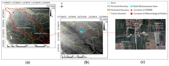
Figure 1.
(a) Location of the Xifei River Basin; (b) location of Lixin County; (c) location of smart soil moisture monitoring instrument (SSMMI).
2.2. Data Acquisition
2.2.1. Data for the DHSVM
The DHSVM input files included the digital elevation model (DEM) data, soil type, land use type, river network data, flow direction data, and meteorological data. The DEM data included a 90 m resolution Shuttle Radar Liner Mission DEM dataset and a 30 m resolution ASTER Global DEM dataset downloaded from the China Geospatial Data Cloud website. The types of soil data were obtained from the website of the Institute of Soil Science, Chinese Academy of Sciences. The map of land use types was extracted from Gaofen-1 (GF-1) satellite images downloaded from the website of the China Resources Satellite Application Center. The river network and flow direction data were based on the DEM and analyzed by ArcGIS software. The meteorological data of a single grid were interpolated from the monitoring data of three meteorological stations, Lixin, Shangqiu, and Kaifeng, and the data of meteorological stations were obtained from the daily dataset of the China Meteorological Data Service Centre.
2.2.2. Satellite Data
Sentinel-1 imagery data were used to retrieve the soil surface moisture area. The Sentinel-1 data were downloaded from NASA’s Earth Science Data Program and pre-processed to eliminate interference. GF-1 satellite data were used for normalized difference vegetation index (NDVI) calculation and crop planting structure extraction.
2.2.3. Field Measured Data of Soil Moisture
The measured soil moisture data for calibration and verification were obtained from the smart soil moisture monitoring instrument (SSMMI) installed in Lixin County. The smart soil moisture monitoring instrument is based on the principle of dielectric constant and frequency domain reflectometry [35]. The instrument can monitor soil moisture and temperature dynamically, and comprehensively analyze soil moisture and environmental meteorological information at different depths. The instrument can be used to deeply study soil and crop root water consumption, and its accuracy can reach ±2%. Two instruments were installed in the study area at Location A (33°13′57″ N, 116°11′39″ E) and Location B (33°13′49″ N, 116°′07″ E), and the specific locations of instruments are shown in Figure 1c. The instruments were used to monitor the soil surface volumetric water content including the 10 cm depth, 20 cm depth, and 30 cm depth volumetric water content at 1 h intervals. The volumetric soil water content data obtained by the DHSVM were the average values of the 0–30 cm layer. The averaged values of four soil layers monitored by the instruments were used for comparison with the simulated values. The dates from 25 August 2020 to 31 December 2020 were selected as the rating period of the model. The dates from 1 January 2021 to 31 June 2021 were selected as the validation period of the model.
3. Methods
This section presents the profile of the DHSVM, the parameter optimization method, the remote sensing (RS) inversion, the method of assimilating RS inversion data into the DHSVM, and the identification criterion of waterlogging damage.
3.1. The Profile of DHSVM
Being a fundamental hydrological model, the DHSVM is a spatially distributed, physics-based hydrology model based on the principle of energy balance and water balance. It takes into account the hydrological interaction and feedback mechanism of rainfall, light, temperature, vegetation, soil, and snow. There are seven computing modules, including the double canopy evapotranspiration module, upper canopy snow melt module, surface snow and snow melt module, unsaturated soil mid-flow module, saturated soil mid-flow module, surface runoff module, and river confluence module. The mass balance equation used for each grid cell in DHSVM [22] is expressed as:
where ΔSS1, ΔSS2, and ΔSSn refer to the variation in water storage in each soil layer (m3) and ΔSio and ΔSiu represent the variation in water storage in each canopy of plants in a single grid (m3). ΔW is the variation of snow cover (m3); P is the external water accepted by the cell, including precipitation (mm) and water obtained from the upstream (m3); ES, Eio and Eiu are the evaporation of soil, vegetation canopy, and lower canopy (m3). Eto and Etu are the transpiration of the upper and lower canopy of vegetation (m3), and P2 is the outflow water of cells (m3).
ΔSS1 + ΔSS2 + … + ΔSSn + ΔSio + ΔSiu + ΔW = P − Eio − Eiu − Eto − Etu − ES − P2
The Nash–Sutcliffe efficiency coefficient was used to evaluate the results of the model.
The NSE formulate can be expressed as:
where is the actual observed soil volume moisture and is the soil volume moisture simulated by the model. is the mean of the measured soil moisture. The NSE ranges from negative infinity to 1, and a zero value of NSE means that the simulation results are close to the average level of measured values. The closer the NSE is to 1, the better the simulation quality of the model is. When NSE is far less than 0, the model is not credible. It is generally believed that when NSE is greater than 0.5, the result is excellent.
3.2. Parameter Optimization for the DHSVM
It is important to conduct the parameter optimization steps including sensitivity analysis, calibration, and optimal spatiotemporal resolution selection on the DHSVM model, because uncertainty in model parameters increases as the model running-time goes on and affects the model outputs [36]. The sensitivity of numerous DHSVM parameters is analyzed to determine which parameters have a great impact on the model. The highly sensitive parameters are calibrated to get the optimal value. The appropriate spatial resolution of DEM data and temporal resolution of meteorological data were selected to simulate the complex physical processes [37]. The optimal spatiotemporal resolution was set by comparing different NSE values of different spatiotemporal resolutions. The parameter sensitivity analysis and calibration methods are introduced in the following sections.
3.2.1. The Parameter Sensitivity Analysis
The parameters in the DHSVM model mainly include global parameters, vegetation parameters, and soil parameters. The global parameters, which include the decline rate of precipitation, the decline rate of temperature, and other parameters, are the spatial attributes of the basin. Since these global parameters are considered constants in the study, we did not conduct sensitivity analysis on global parameters. In crop areas, the changes in vegetation and soil parameters were mainly considered, and the extended Fourier amplitude sensitivity test (EFAST) method was used to analyze the sensitivity of vegetation and soil parameters.
The EFAST method adopts the idea of model variance analysis and is a global sensitivity analysis method combining the Sobel method and Fourier amplitude sensitivity test. The first-order sensitivity indices and the total sensitivity indices of the input parameters can be obtained by establishing the search curve to convert a multidimensional integral of all the input variables to a one-dimensional integral [36].
The variance of input variables and the variances of the interaction among the variables contribute to the total variance of model outputs. The first-order sensitivity index reflects the direct contribution of the variable to the total variance of model output. Both the first-order sensitivity index and the higher-order sensitivity indices of variables can be obtained by normalization:
where V is the total variance of the model output, Vi is the variance of variable i, Vij is the variance of the interaction between variables i and j, Vijm is the variance of interaction among variables i, j, m. Si is the first-order sensitivity index, and Sij and Sijm are the higher-order sensitivity indices.
Si = Vi/V, Sij = Vij/V, Sijm = Vijm/V
The sensitivity index reflects the direct contribution rate of parameters to the total variance of the model outputs. The total sensitivity can be expressed as:
STi = Si + Sij + Sijm + … + S12…i…k
The total sensitivity index reflects the sum of the direct contribution rate of parameters and the indirect contribution to the total variance of the model output through the interaction and coupling with other parameters. The total sensitivity reflects the influence of parameter changes on the model and determines the parameters with higher sensitivity.
3.2.2. The Parameter Calibration
The PSO algorithm [38] is used as the parameter calibration method in this study. The PSO algorithm has several advantages, such as easy implementation, fewer parameter settings, and fewer iterations [39]. Each particle is given two attributes: position and velocity. Each particle separately searches for the optimal solution in the search space, which is recorded as the current individual extreme value. The individual extreme value is shared with other particles in the whole particle swarm. The optimal individual extreme value is treated as the current global optimal solution of the whole particle swarm. All particles in the particle swarm adjust their velocity and position according to the current individual extremum and the current global optimal solution.
The number of the particle swarm is set as N, the count of sensitive factors is set as D, the number of iterations is set as A, and the maximum velocity is set as vimax. The initial position and velocity of each particle is defined as xn,d, vn,d respectively, where the swarm number n belongs to [1, N], and the sensitive factors number d belongs to [1, D]. These initial positions and velocities are randomly defined within the range of allowable values. The specific steps are as follows.
- The particle swarm settings are input to the DHSVM to calculate the fitness of these settings.
- Each particle’s best fitness setting Pbest is compared to update the group particle best fitness Gbest.
- The positions and velocities are updated, and the value beyond the boundary needs to be adjusted. It can be expressed as:where ω is the inertia weight, which is the number of [0, 1]; c1 and c2 are acceleration coefficients, which are usually fixed at 2.0; and r1 and r2 are random numbers in [0, 1].
- Iterating to the maximum number or NSE coefficient meets the requirements.
3.3. Remote Sensing Inversion Method of Soil Moisture Data
The water cloud model (WCM) is used for the remote sensing inversion of soil moisture. It is a vegetation contribution model applied in soil moisture retrieval over vegetated areas. The model suggests that the scattering echo is accepted by the radar sensor due to the scattering between vegetation and soil. It assumes that the layer of vegetation water is evenly distributed. WCM simplifies the complex scattering effect between the vegetation layer and soil layer. WCM removes the influence of vegetation on the backscattering coefficient and obtains the total backscattering coefficient from the vegetation scattering coefficient and soil surface backscattering coefficient. The specific steps are as follows.
1. The backscattered radar signal in linear scale (σ0) is defined as the sum of the contribution of the vegetation canopy (), the scattering from the soil layer (), and soil–vegetation scatterings. The soil–vegetation interactions in the WCM are neglected for simplicity. The WCM formulations are listed in the following.
where V1 and V2 are the vegetation’s descriptors. The values of vegetation parameters A and B are 0.0018 and 0.138, which are acquired directly from Bindlish et al.’s study [40]. Bindlish et al. offer different land-cover vegetation parameters including for winter wheat, and consider that V1 is equal to V2, and also the vegetation water content. Therefore, although several parameters such as vegetation water content (VWC), leaf area index, and the NDVI can be used as the vegetation’s descriptors [41], VWC is used as V1 and V2 in our study. Moreover, VWC is calculated according to the empirical model of Jackson [42].
2. According to the incident angle, vegetation moisture, and total backscattering coefficient, the soil backscattering coefficient considering crop cover is calculated under the condition of VV polarization. After converting the unit of backscattering coefficient into the decibel unit in Equation (10), we used the linear function to invert the SAR soil backscatter into soil moisture values in Equation (11).
where is the soil backscattering with the unite of decibel (db); SM is soil moisture; and C and D are empirical coefficients (slope and intercept) in different phenological stages.
Through field investigation in the study area, we determined that winter wheat is sown in October and harvested in June next year. The growth period of winter wheat is divided into the following: sowing time, tillering stage, overwintering period, returning green stage, jointing stage, heading stage, milky stage, and maturity stage. Water requirements of winter wheat are different in different phenological stages. In our study, according to the water requirement changes, the whole growth period was divided into three phenological stages: sowing–tillering, overwintering, and greening–maturity stages. We also built the linear relationship between the backscattering coefficient and soil moisture based on the above three phenological stages, and Equation (11) is a piecewise linear function. The empirical parameters C and D are different in different stages and Table 1 shows the values of C and D parameters acquired from Zhang et al.’s study [9].

Table 1.
Values of C and D parameters during different phenological stages.
3. In conclusion, the soil moisture content is calculated by combining the phenological characteristics of specific crops in the study area. The distribution of soil moisture content is obtained by establishing the relationship between the backscattering coefficient and surface soil moisture content. The specific remote sensing inversion method based on crop phenological traits is shown in Zhang et al.’s study [9].
3.4. The Agro-Hydrological Assimilation Model for Winter-Wheat Waterlogging Monitoring
According to our field investigation and Shi’s research [43], winter wheat is grown on a large scale in Lixin County, and the irrigation system of farmland is adjusted according to the annual rainfall. Since the complex artificial irrigation and drainage system in farmland has a great influence on soil moisture content, the actual soil moisture content distribution is difficult to obtain by the hydrological model only. Meanwhile, the remote sensing (RS) inversion method based on satellite images has the advantage of clearly reflecting the spatial distribution of soil moisture at the specific moment. In order to give consideration to both the hydrological model’s and the RS inversion method’s advantages, we built an agro-hydrological assimilation model for winter-wheat waterlogging monitoring by assimilating RS inversion data into the DHSVM hydrological model.
The assimilation method for the agro-hydrological assimilation model was the successive correction method proposed by Cressman [34]. The assimilation process includes the following steps: (1) the initial values of grid points are given by the simulation results; (2) the next step is calculating the increment of each point between the value obtained by RS inversion and the initial value within the influence radius; (3) different weights are given to the increments within the influence radius, and then the increment is added to the initial value to obtain the revised soil moisture content distribution; (4) the previous steps are iterated.
The iterative formula is expressed as:
where is the value of the ith grid point after n iterations, is the bth observation point within the influence radius of grid point i, is the nth estimation of observation point b, and is the total number of observation points within the influence radius.
The original method of determining weights for successive correction is a quadratic weight function inversely proportional to the square of the distance. In our study, the unit of the distance was the meter. Barnes [44] adds the convergence factor to the Gaussian distribution weight in order to obtain a new weight function, which was used in the study. The convergence factors are expressed as:
where is the square of the distance between observation point b and grid point i, R is the radius of influence, and the convergence factor γ is 0.5, iterating twice in total.
3.5. The Identification Criterion of Waterlogging Damage Distribution
Since waterlogging damage in farmland soil is caused by excessive soil water in the upper layer continuously over a long time [3], the time-continuous feature is considered when extracting waterlogging damage. In this paper, the average value of soil moisture content for five consecutive days was used as the fifth day’s value. Thus the soil moisture content value every day was reassigned as the above average value. It was defined as the standard for marking waterlogging damage at a specific grid point that the moving reassignment value of soil moisture content was greater than 95% for five consecutive days [14]. This waterlogging extraction method avoids the misjudgment of waterlogging damage due to the abnormal value of a certain day. Two further extraction methods were used to evaluate the disaster degree of waterlogging damage, which are as follows.
(1) Waterlogging damage ratio calculation by using soil moisture data during winter wheat growth period.
Winter wheat is usually sown in early October and harvested at the end of May on the Huaibei Plain. The simulated soil moisture maps of 243 days from 1 October 2020 to 31 May 2021 were chosen to monitor the waterlogging damaged-ratio distribution in Lixin County. According to the above waterlogging damage standards, the sum of waterlogged days at a certain point was obtained by programming in the IDL language. The waterlogging damage ratio was calculated by the following formula.
where n is the sum of waterlogged days, and N is the total number of days of crop growth.
R = n /(N − 8)
The daily soil moisture content for waterlogging monitoring was the five-day moving average value. The actual soil moisture values from 1–5 October 2021 were used to calculate the moving average value of 5 October 2021. Therefore, the date of soil moisture average values used for winter-wheat waterlogging extraction was from 5 October 2021. Moreover, the occurrence of waterlogging damage requires that the soil moisture content exceed the standard for at least five days. Therefore, the first occurrence date of waterlogging damage was from 9 October 2021. Eight was subtracted from N in Equation (14).
The study areas were consequently classified as having four waterlogging-damaged ratios: extremely low damaged-ratio areas (R less than 0.1), low damaged-ratio areas (R greater than 0.1 and less than 0.3), medium damaged-ratio areas (R greater than 0.3 and less than 0.6), and high damaged-ratio areas (R greater than 0.6).
(2) Grade distribution extraction of waterlogging damage by using soil moisture data during certain periods with heavy rain.
The grade distribution of waterlogging damage was used for evaluating the disaster degree of the study area during certain periods with heavy rain. The average soil moisture data during certain periods with heavy rainfall from 1 May to 17 June 2021 were input into the IDL program to make the change process map of waterlogging damage grade distribution. The disaster degree distribution maps from 7–17 June 2021 were finally recorded as a result of the waterlogging accumulation characteristics. The grades of the waterlogging damage degree depended on how long the moving average value of soil moisture content continuously exceeded 95%, which are as follows: mild waterlogging damage (more than 5 days and less than 12 days), moderate waterlogging damage (more than 12 days and less than 20 days), and severe waterlogging damage (more than 20 days).
4. Results
4.1. The Parameter Optimization Results of the DHSVM Model
4.1.1. Results of Parameter Sensitivity Analysis
There were eleven parameters for the sensitivity analysis by EFAST, including the lateral conductivity, maximum infiltration, field capacity, Manning coefficient, wilting coefficient, pore size distribution, bubbling pressure, leaf area index, vegetation albedo, critical humidity, and minimum stomatal resistance. A total of 715 combinations for the above eleven parameters were produced by EFAST analysis in order to simulate soil moisture in Lixin County. Since the model inversion error gradually accumulated as the simulation time increased, we used a shorter simulation time to determine the sensitivity of the model parameters. The simulation time period was from 25 August 2020 to 6 September 2020. The simulation results were used to analyze the first-order sensitivity and global sensitivity of the parameters. The first-order sensitivity is the sensitivity when the value of a single parameter is changed separately, and the total sensitivity refers to the sensitivity when parameters are correlated with each other. Sensitivity analysis results of parameters are shown in Table 2.

Table 2.
Parameter sensitivity.
The first-order and the total sensitivity indexes were calculated for each input variable, and the total sensitivity indexes were used for the sensitivity analysis of parameters in the study. According to Table 2, the vegetation parameters such as the vegetation albedo, leaf area index, and minimum stomatal resistance, the soil parameters such as the lateral hydraulic conductivity, field water holding capacity, and wilting coefficient have high global sensitivity to soil moisture. Therefore, the above six most sensitive parameters were selected according to the EFAST total order index, and are further calibrated in Section 4.1.2. The parameters of vegetation albedo, leaf area index, lateral conductivity, field capacity, wilting coefficient and minimum stomatal resistance need to be calibrated.
4.1.2. Results of Parameter Calibration
The PSO algorithm was used for calibrating six parameters: vegetation albedo, leaf area index, lateral conductivity, field capacity, wilting coefficient, and minimum stomatal resistance. The soil moisture data used for calibration were the field measured data at the SSMMI A and B locations in Lixin County from 25 August 2020 to 1 January 2021. The NSE of simulation results at two SSMMI locations was taken as the fitness function. In the study, the PSO algorithm set the population number as 10, and the number of iterations as 20. The absolute value of the maximum velocity of each particle was not greater than 0.2 of the value range of each particle. The range of parameter values and results are shown in Table 3.

Table 3.
Calibration results of parameters.
4.1.3. Results of Spatiotemporal Resolution Selection
After setting the calibrated parameters in the DHSVM model, we ran the model under different spatiotemporal resolution combinations including 90 m+ 24 h, 90 m+ 3 h, and 30 m+ 24 h. We compared the simulation results with field measured values at the SSMMI B location to determine which spatiotemporal resolution was the best combination. The results with different spatial resolutions are shown in Figure 2a, and the results with different temporal resolutions are shown in Figure 2b. The NSE coefficients of the models under different spatiotemporal conditions are shown in Table 4.
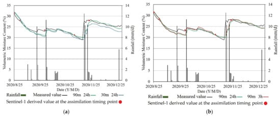
Figure 2.
(a) Simulation results with different spatial resolutions from the SSMMI B location; (b) simulation results with different temporal resolutions from the SSMMI B location.

Table 4.
NSE of each spatiotemporal resolution combination.
We analyzed the spatiotemporal resolution selection two ways. (1) First, the temporal resolution of weather data was fixed on 24 h, and the results with different spatial resolutions were compared. When the temporal resolution was 24 h, under the same parameter combination, DEM data of 30 m and 90 m were put into the model. As Figure 2a shows, the results indicate that there was no obvious difference between the two simulation results from two spatial resolution inputs at the early stage of the model operation, while the model with 90 m resolution input performed better than that with 30 m resolution input in the latter half stage. Then DEM data with 90 m were selected for the model. (2) Second, the spatial resolution of DEM was fixed on 90 m, and the results with different temporal resolutions were compared. When the spatial resolution was 90 m, under the same parameter combination, weather data of 24 h and 3 h were put into the model. As Figure 2b shows, the model using 3 h temporal resolution with 0.73 NSE worked better. Then weather data with 3 h were selected for the model. Finally, the spatiotemporal resolution combination of 90 m + 3 h was selected for the DHSVM.
4.2. The Improvement Effect of the Agro-Hydrological Assimilation Model for Winter-Wheat Waterlogging Monitoring
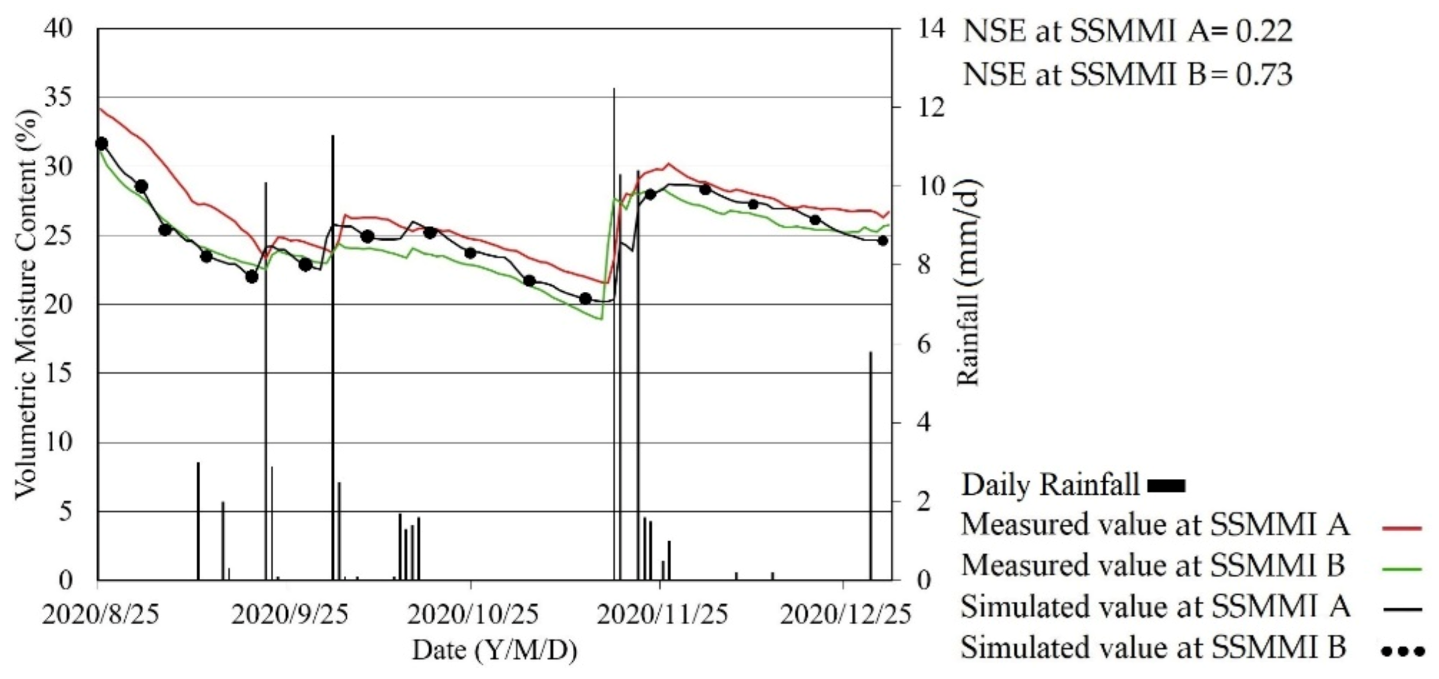
Figure 3 presents the simulation results of soil moisture by the DHSVM model without assimilation. It was found that the simulation values of soil moisture content at two closely spaced locations were difficult to distinguish. The simulated values at SSMMI A and B locations were almost the same without the assimilation, but the measured soil moisture values at two locations were different. It was also found that at SSMMI A and B locations, the change trend of the simulated soil moisture content was the same as that of the measured value, but there was always a certain deviation between the simulated value and the measured value at the SSMMI A location. The reason for this phenomenon may be that the initial values of soil moisture for the DHSVM model without assimilation were the same at each pixel point, which cannot reflect the actual local situation at a certain moment. Meanwhile, as shown in Figure 3, the initial value of soil moisture was closer to the measured value at SSMMI B than that at SSMMI A, so the NSE coefficient at the SSMMI B location was relatively high.
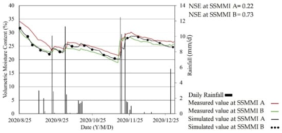
Figure 3.
The simulation results of soil moisture by the DHSVM model without assimilation.
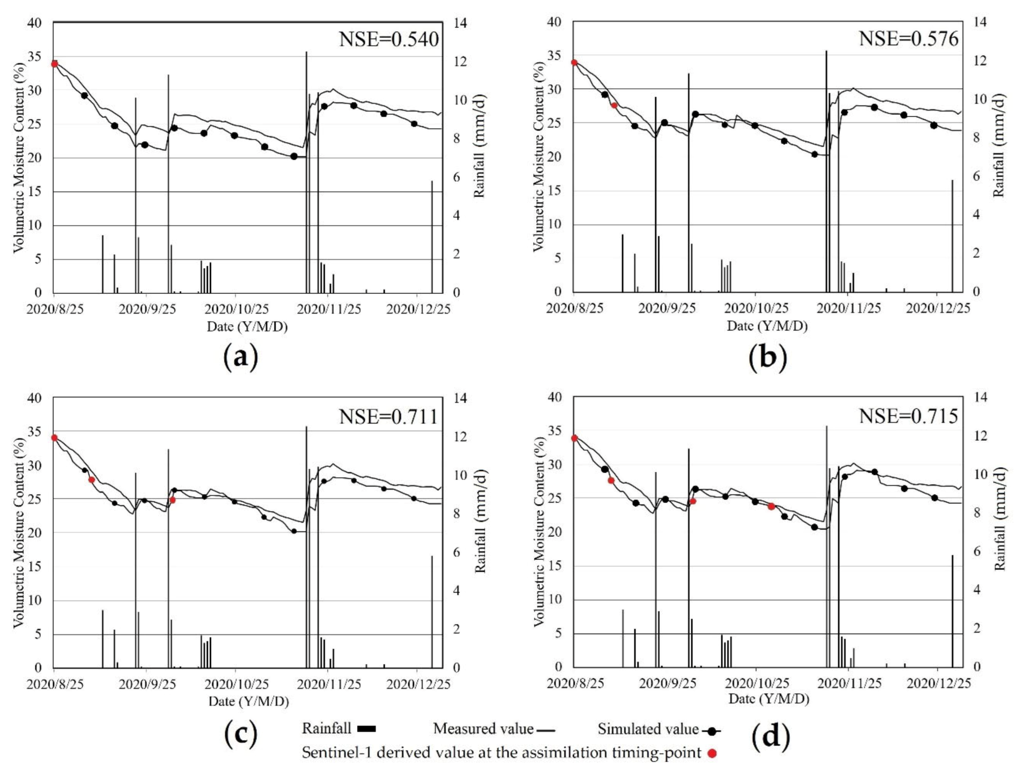
Therefore, this study took the soil moisture maps made using RS inversion as the initial values of soil moisture when running the agro-hydrological assimilation model for winter-wheat waterlogging monitoring. One RS inversion map was assimilated into the DHSVM every month. The improvement effect of the assimilation model is shown in Figure 4.
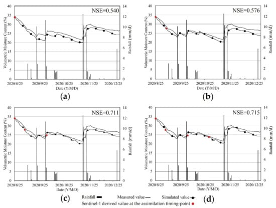
Figure 4.
The improvement effect by assimilating RS inversion maps for SSMMI A. (a) The effect by assimilating one RS inversion map; (b) the effect by assimilating two RS inversion maps; (c) the effect by assimilating three RS inversion maps; (d) the effect by assimilating four RS inversion maps.
Figure 4a–d shows the results of assimilating 1, 2, 3, and 4 inversion maps respectively. The red points in the figure are the timing points when assimilating the RS inversion map. Figure 4a shows that assimilating one RS inversion map into the model effectively made the simulated value close to the measured value during the initial stage. However, it is also shown in Figure 4a that irregular and artificial drainage and irrigation in farmland may affect the simulation results, leading to errors between the simulated values and the measured values during the later stage of running the model. It can be seen from Figure 4 that the simulation results of soil moisture were closer and closer to the measured value with assimilation of an increasing number of RS inversion maps. The corresponding NSE values in four conditions with different assimilation numbers are 0.540, 0.576, 0.711, and 0.715, respectively, which are also higher and higher with an increasing assimilation number.
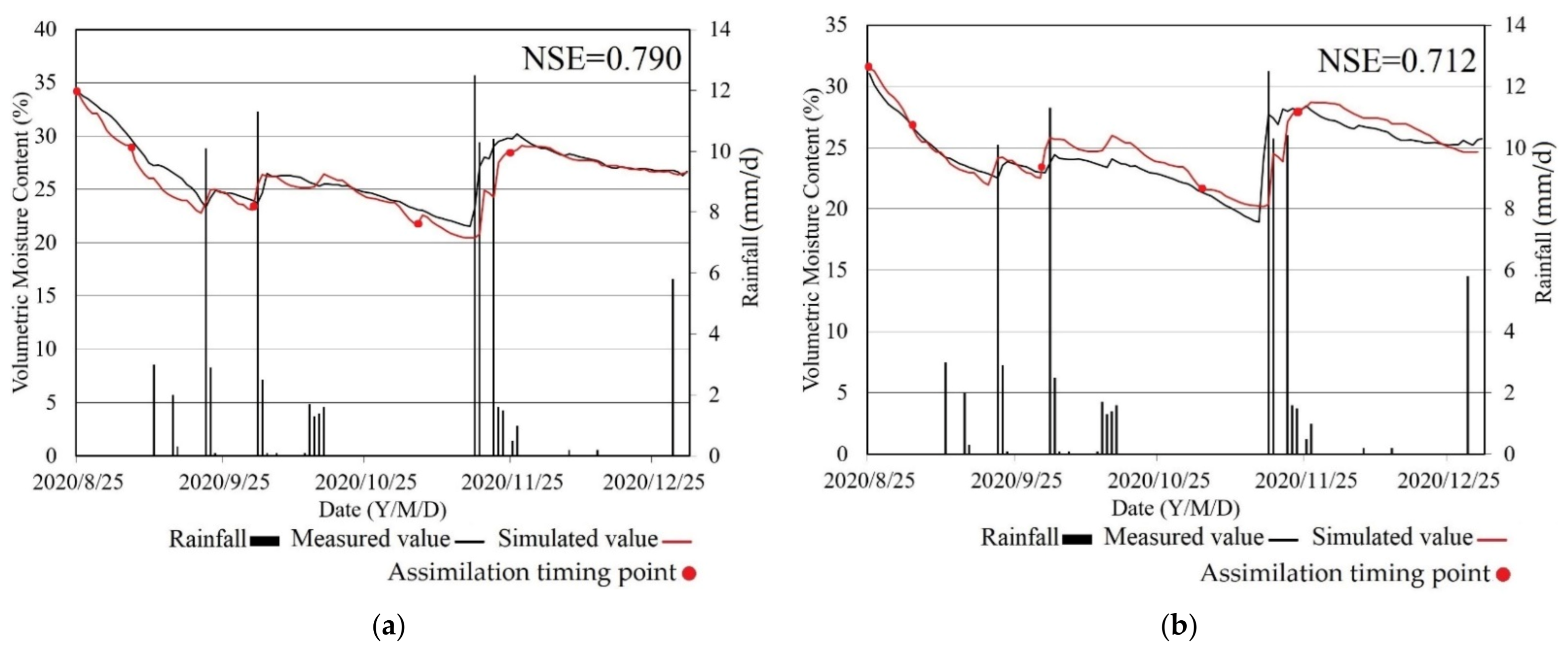
Figure 5 shows the final improvement effect by assimilating five RS inversion maps into the DHSVM. It also shows the comparison between the simulation results of the agro-hydrological assimilation model and the field measured data at two SSMMI locations. From Figure 5, the initial value at SSMMI A was 33.97%, and the value at SSMMI B was 31.47%, which are both close to the corresponding measured values. The difference of the initial values between SSMMI A and B locations is reflected in the agro-hydrological assimilation model. The corresponding NSE values at SSMMI A and B locations were 0.790 and 0.712 respectively, which shows that the simulation effect at two SSMMI locations is good.
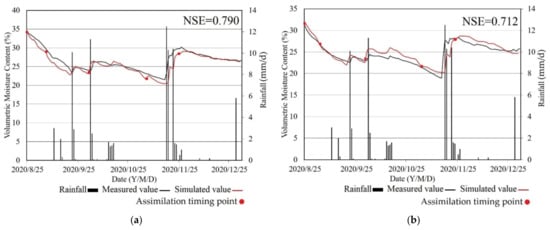
Figure 5.
The final improvement effect of the agro-hydrological assimilation model (a) for SSMMI A and (b) SSMMI B.
4.3. Accuracy Verification of the Agro-Hydrological Assimilation Model for Winter-Wheat Waterlogging Monitoring
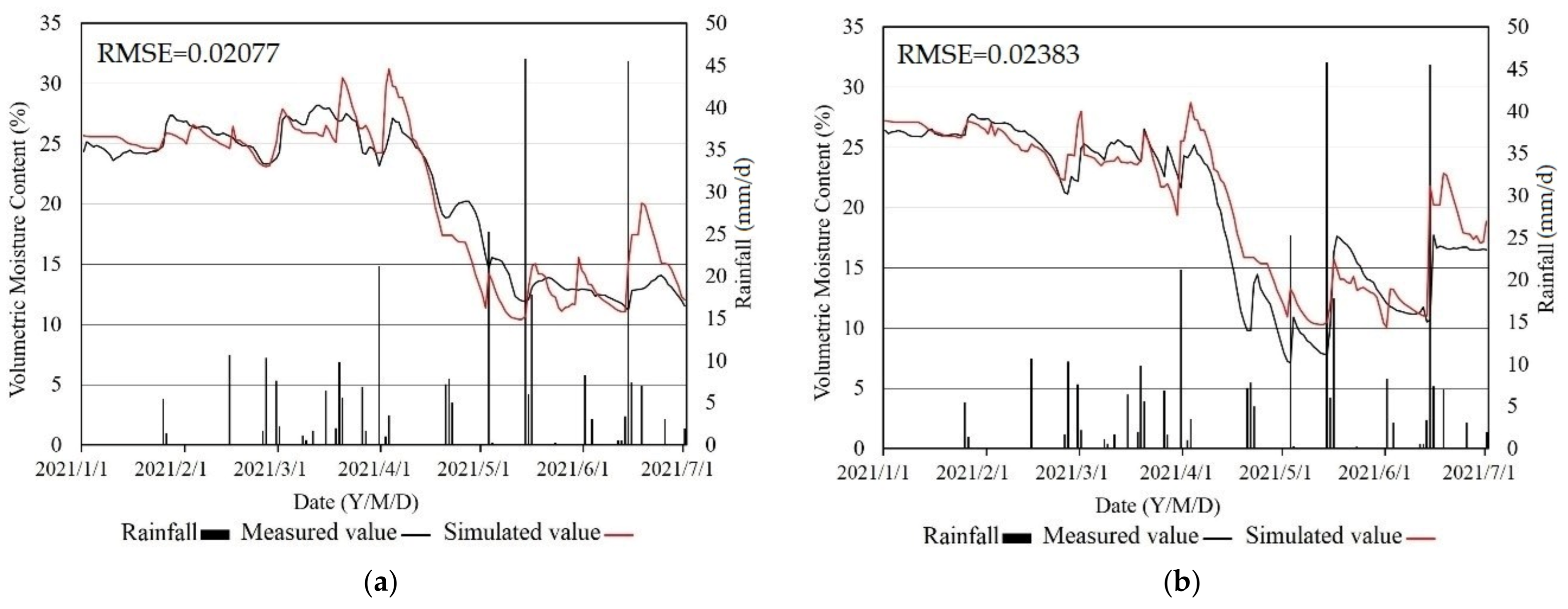
The field measured soil moisture data from 1 January to 31 June 2021 were used as the verification data. The RMSE between the measured data and the simulated values was calculated to assess the accuracy of the agro-hydrological assimilation model. The accuracy verification results are shown in Figure 6. The RMSEs at two SSMMI locations were 0.02077 and 0.02383 respectively, which were 9.96% and 12.02% of the measured data.
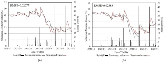
Figure 6.
The accuracy verification of the agro-hydrological assimilation model (a) for SSMMI A and (b) SSMMI B.
4.4. The Soil Moisture Distribution Results by the Agro-Hydrological Assimilation Model
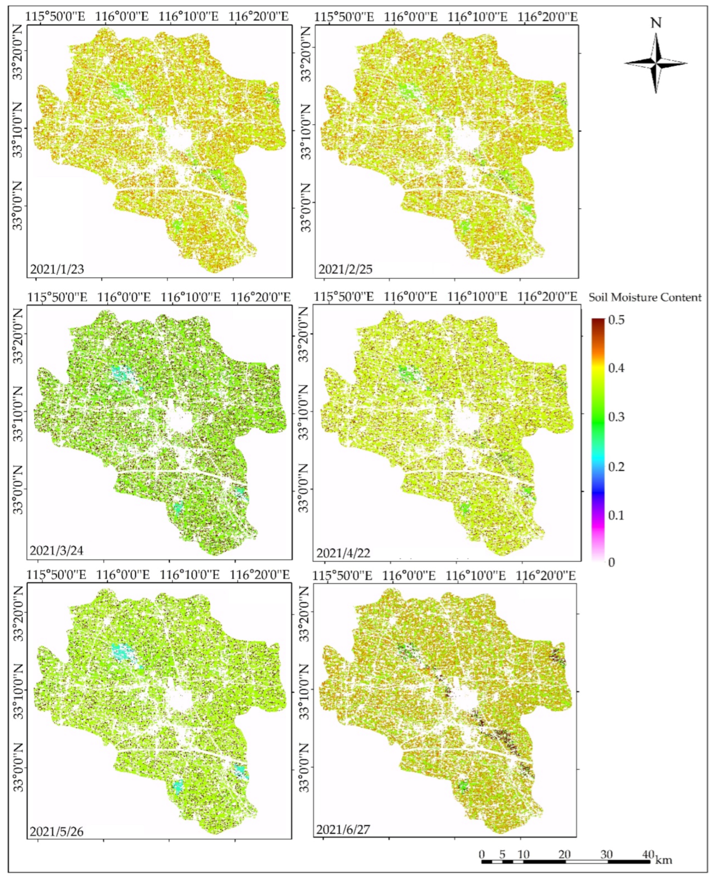
The soil moisture distribution maps in Lixin County from January to June 2021 were simulated by the agro-hydrological assimilation model for winter-wheat waterlogging monitoring. In Figure 7, parts of the soil moisture simulation maps are presented as examples.

Figure 7.
The monthly samples of soil moisture distribution results from the agro-hydrological assimilation model in Lixin County.
The soil moisture contents in Lixin County were high from January to February in 2021. The reason may be that the region during this period was in a relatively cold winter, and the evapotranspiration of soil and crops was low. With the arrival of spring, the soil moisture content in Lixin County decreased to a lower level from March to May. During this period, with increasing temperature, the evapotranspiration of soil and crops increased correspondingly. The soil moisture content increases in summer, which is consistent with the climate characteristics of abundant summer rain in Lixin County. The soil moisture content of Lixin County was even in the spatial distributions, which is consistent with Lixin County’s flat topography.
4.5. Monitoring Results of Damaged Ratio and Grade Distribution for Winter-Wheat Waterlgging
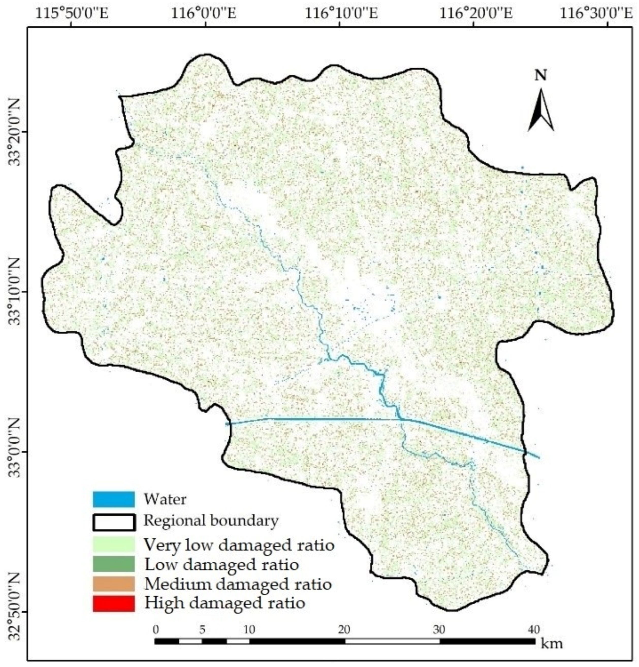
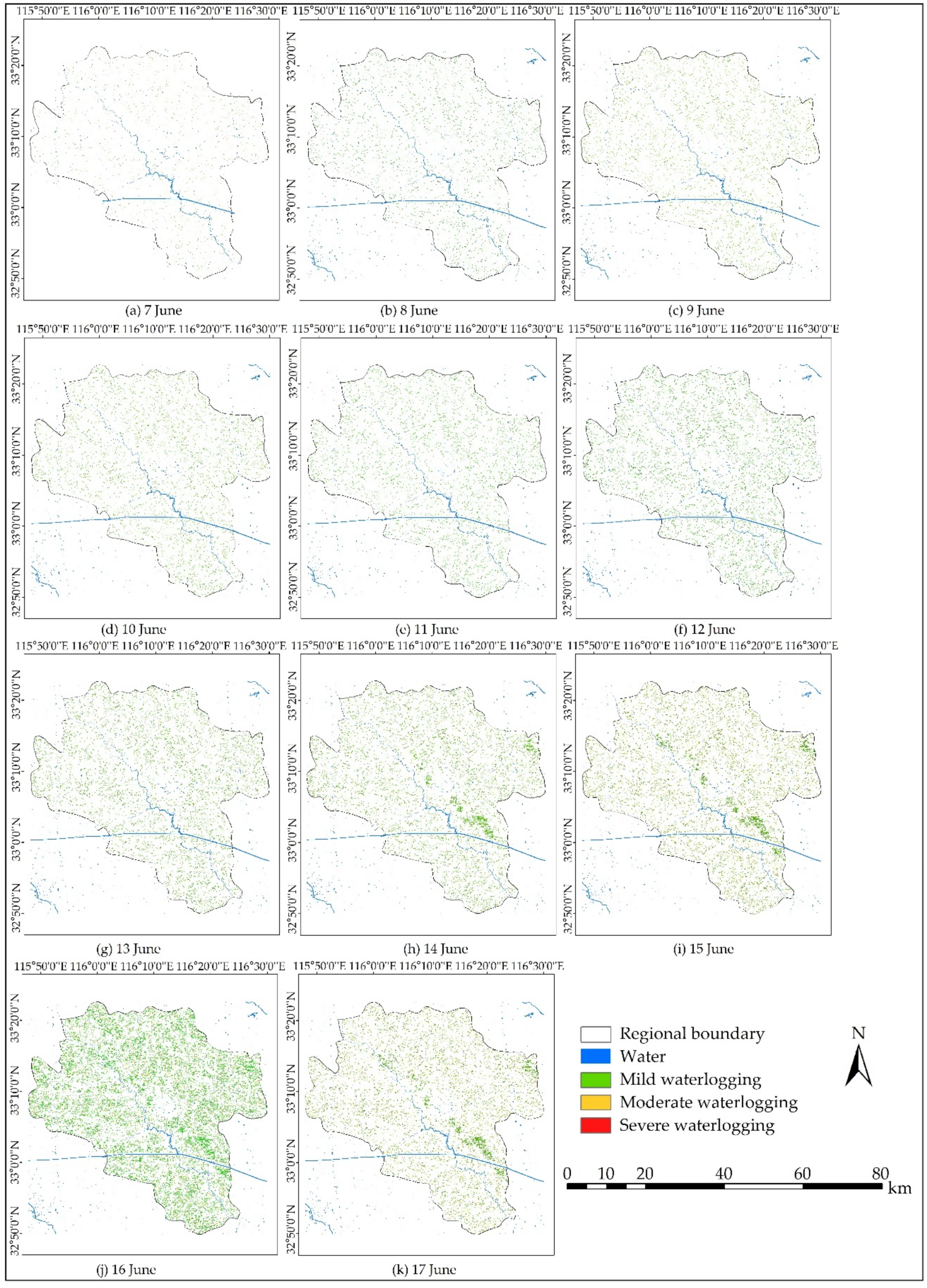
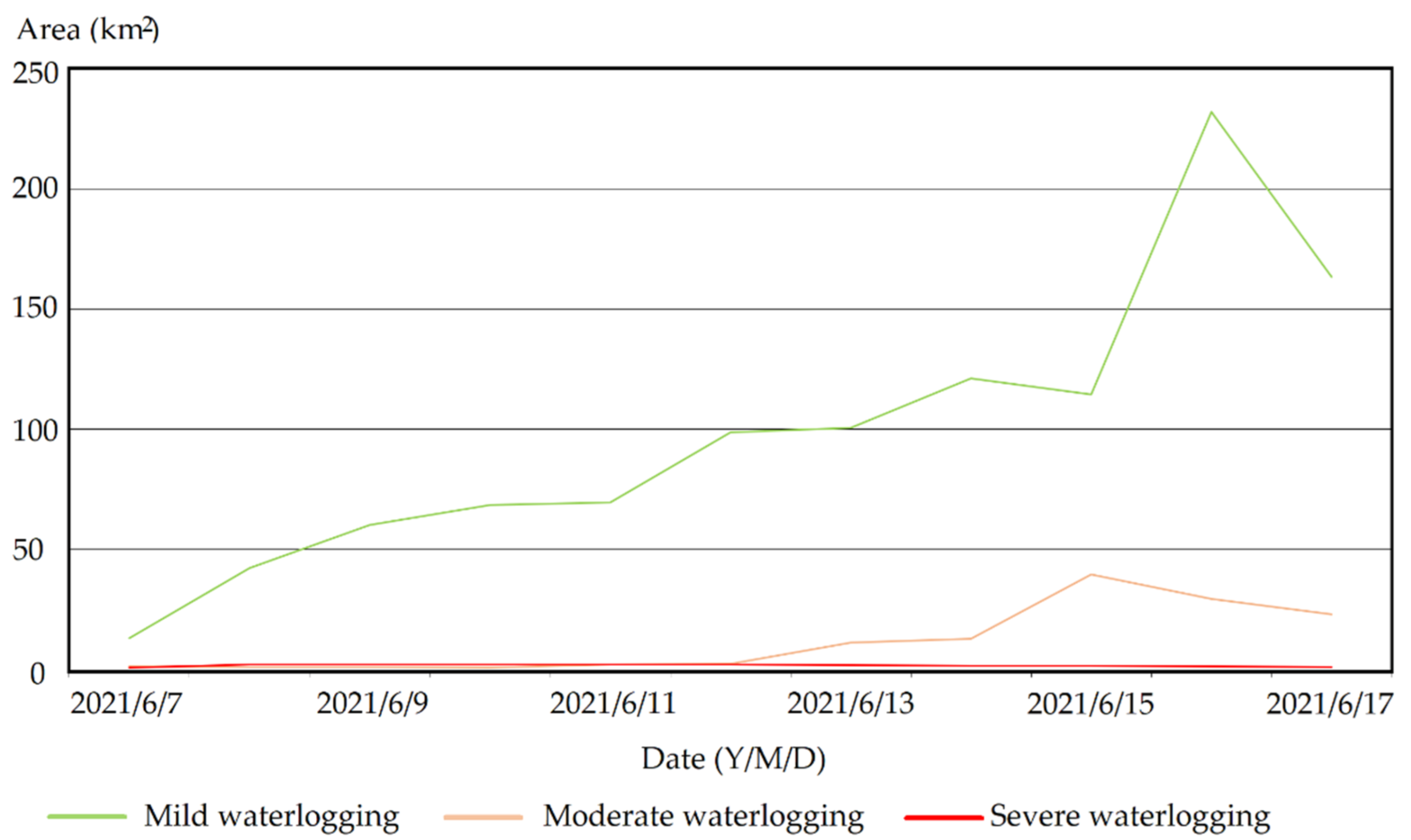
The winter-wheat waterlogging monitoring results include the damaged ratio and grade distribution of waterlogging damage. The daily soil moisture results by the agro-hydrological assimilation model were input into the Interactive Data Language (IDL) program to obtain the waterlogging damaged ratio map during the wheat growth period from October 2020 to May 2021, as shown in Figure 8. The area of each ratio level is shown in Table 5. The IDL program was also used to obtain the grade distribution of waterlogging damage from 7–17 June 2021 during the period of abundant rainfall, as shown in Figure 9. The area change of the three damage grades is shown in Figure 10.
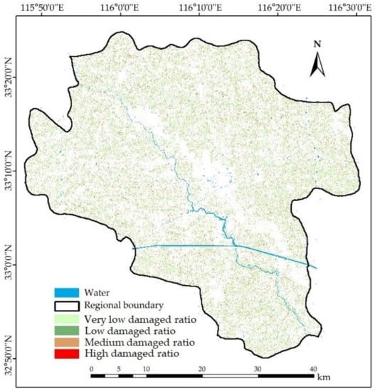
Figure 8.
The waterlogging damaged ratio map during the wheat growth period from October 2020 to May 2021.

Table 5.
Area of four damaged ratio levels.
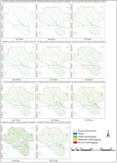
Figure 9.
Grade distribution maps of waterlogging damage from 7–17 June 2021.
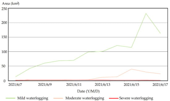
Figure 10.
The area change of three damage grades from 7–17 June 2021.
From the damaged ratio distribution map (Figure 8) and the area of damaged ratio levels (Table 5), it was found that the damaged ratio level in most of the study area was very low, and a small number of medium damaged ratio areas was mixed, which indicates that the difference of spatial distribution in Lixin County is not obvious.
From the grade distribution maps (Figure 9) and the area change of damage grade (Figure 10), it can be found that during the abundant-rain period, the waterlogging damage grade in most of study area was mild waterlogging damage, which indicates that the local drainage conditions were good and the surface ponding water was drained in time.
5. Discussion
5.1. Parameter Optimization Analysis of the DHSVM Model
As shown in Table 2, the vegetation albedo, leaf area index, transverse hydraulic conductivity, and field capacity had high sensitivity in the DHSVM model. In Zhao et al.’s research about a cold alpine basin, the most sensitive parameters in order were the transverse hydraulic conductivity, field capacity, leaf area index, and vegetation albedo [45]. The order of the parameter sensibility was different from that in our study. The reason may be that the climate and the planting structure in our study area were different from Zhao et al.’s. During the crop growth period in Lixin County, crop growth changes greatly, and soil moisture changes little. However, in Zhao et al.’s high cold mountain study area, soil moisture also changed greatly during the crop growth period. Therefore, vegetation parameters are more sensitive than soil parameters in Lixin County.
In Figure 2, when the model had the same parameters and temporal resolution, the model result using DEM data with 90 × 90 m resolution was better than that using DEM data with 30 x 30 m resolution. In a study about the DHSVM, Amorim et al. also found that the simulation accuracy decreases when the spatial resolution is more accurate [46]. Indicators such as NS, PBIAS, and RMSE of the model with a resolution of 100 x 100 m are better than those with a resolution of 45 × 45 m. There is no positive correlation between high spatial resolutions and excellent results. For different environmental factors, the optimal spatial resolution of DEM was different. The DHSVM had no strict requirements for the spatial resolution. DEM with a low spatial resolution does not lead to results with low accuracy.
5.2. Influence Factors Analysis on the Agro-Hydrological Assimilation Model for Winter-Wheat Waterlogging Monitoring
5.2.1. The Model Uncertainty Analysis
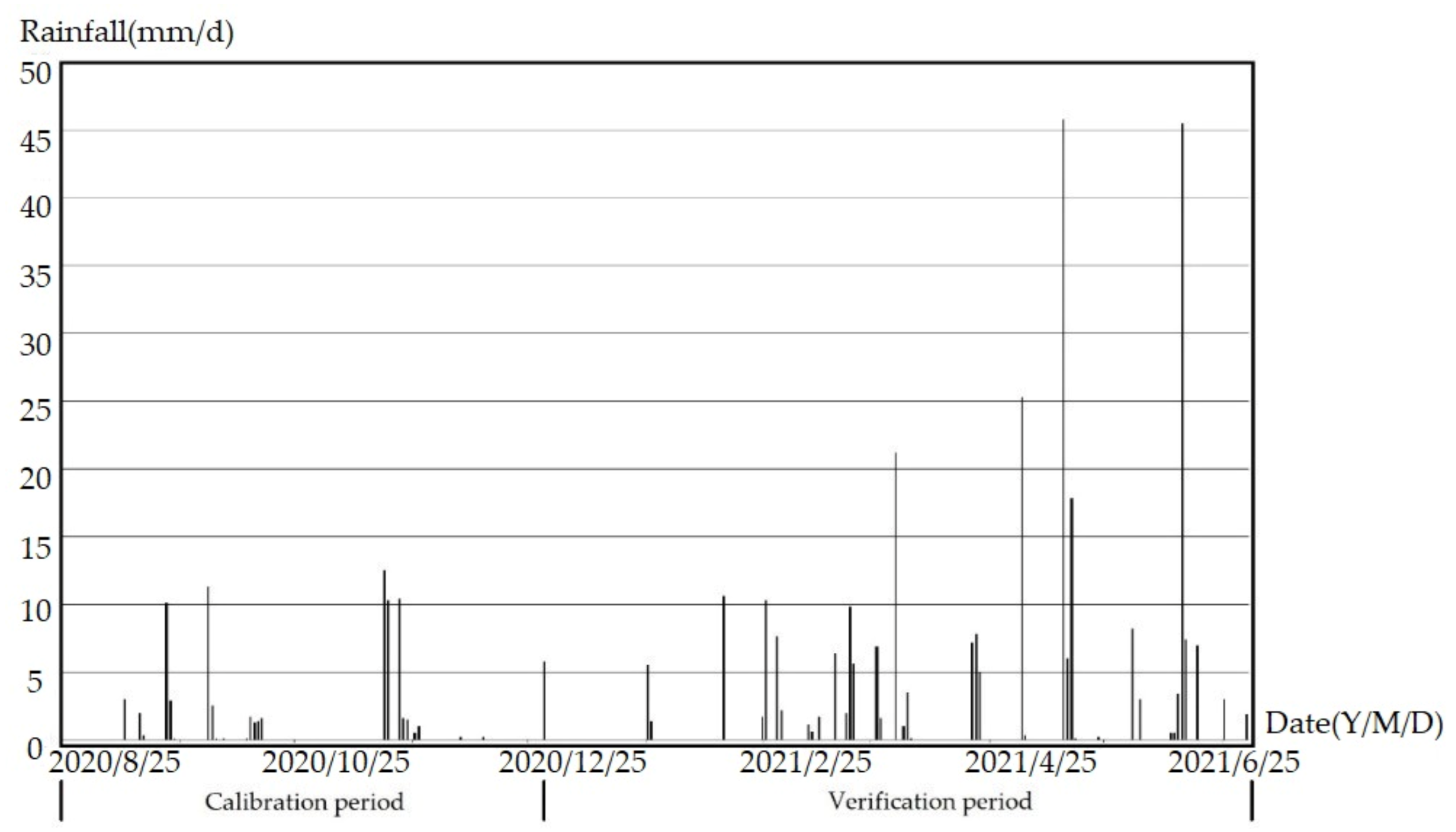
The calibration period for the agro-hydrological assimilation model was from 25 August to 31 December 2020, and the validation period was from 1 January to 31 June 2021. In Figure 6, during the validation period, the simulation accuracy from January 1 to March 31 was better than that from 1 April to 31 June 2021. From Figure 11, the average daily rainfall of the validation period from 1 January to 31 March 2021 did not exceed 0.02 m, and this rainfall intensity was similar to the rainfall data of the calibration period. However, the rainfall increased significantly from 1 April to 31 June 2021, and the average daily rainfall on 14 May and 14 June exceeded 0.045 m. This rainfall intensity was different from that in the calibration period, which led to lower simulation accuracy from 1 April to 31 June than that from 1 January to 31 March 2021, and indicates that excessive rainfall may reduce the simulation accuracy.
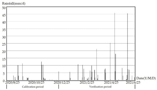
Figure 11.
Daily rainfall during the calibration and verification period.
The terrain in Lixin County, with a gentle slope, leads to difficult water drainage by gravity. The lime-concretion black soil is also not conducive to the infiltration of water. Under these two natural conditions, when a large rainfall event occurs, the soil moisture content is relatively high and this will last for a long time, which may lead to waterlogging disasters in some areas. In recent years, many artificial drainage facilities have been built in Lixin County, which effectively drain water when a surge in rainfall occurs. However, it is difficult to consider all artificial measures when running the agro-hydrological model. Therefore, as shown in Figure 6, the measured soil moisture content is far less than the simulated soil moisture content after heavy rain. Schulz et al. also found that the decrease of soil moisture content using artificial drainage is faster than that under natural drainage conditions [47]. Eekhout et al. [48] indicate that the uncertainty of the DHSVM model increases with extreme precipitation and runoff. These research efforts stress the importance of considering artificial drainage factors when running agro-hydrographic models such as the DHSVM in order to reduce the model uncertainty.
5.2.2. Influence Analysis of Assimilating Remote Sensing Inversion Data
As shown in Figure 3, when RS inversion maps are not assimilated into the DHSVM, the trend of the simulated values is the same as with the measured values, but there is a gap between the simulated and measured values at the SSMMI A location. The initial value for the DHSVM model without assimilation at this location was not coincident with the actual measured value. Yu tries to make the simulated values of soil moisture content more consistent with the measured values based on local DEM and meteorological data [49]. However, irrigation, drainage, and other artificial measures are not included in the model simulation process. The large number of farms and artificial ditches in the study area led to a deviation between the simulation results and the actual soil moisture content. Moreover, the errors accumulated continuously in the model simulation process. Therefore, it is necessary to assimilate remote sensing inversion data reflecting the real-time surface values into the agro-hydrological model.
As shown in Figure 4a, when a RS inversion map was assimilated as the initial value for the model, the simulated value was accurate at the beginning of the model operation. However, after the model was running for a while, with the accumulation of errors, the model simulation accuracy decreased. This phenomenon indicates that one RS inversion map used for the agro-hydrological assimilation model is not sufficient. Therefore, it is necessary to assimilate sufficient RS inversion maps to reduce the model uncertainty.
5.3. Analysis of Waterlogging Damage Results in Lixin County
Lixin County was evaluated as a high waterlogging damaged-ratio area from 2001 to 2010 according to the Huaihe Basin’s research report [4]. Meanwhile, in the report, the vulnerability risk of carriers in Lixin County was also evaluated as a high level, due to the wide cultivated land area and the high planting proportion of dry crops. The local agricultural output value accounted for a large proportion of the Lixin economy and was very vulnerable to waterlogging disasters according to the Huaihe Basin’s research report. However, according to the waterlogging monitoring results from 2020 to 2021 in our research, most of the areas with waterlogging damage had a very low damage ratio. Results from the small number of medium damaged-ratio areas were mixed, and do not show obvious regional distribution differences. It can also be seen from the grade distribution maps of waterlogging damage (Figure 9) that the waterlogging damage in Lixin County was mild during the period of abundant rainfall. By comparing the previous Huaihe Basin research with the present Lixin study, it was found that the local drainage conditions have improved and the local waterlogging damage has been effectively controlled. There are almost no high waterlogging damaged-ratio areas, and no severe waterlogging damage areas. According to our field investigation in June 2021, there was no serious waterlogging in Lixin County in 2021, which is consistent with the simulation results. Moreover, the drainage project construction has been completed, and the above average waterlogging caused by rainstorms has been reduced according to the farmland drainage standard.
6. Conclusions
Waterlogging monitoring needs to consider the continuity of features present in farmland soil affected by waterlogging disasters. We developed an agro-hydrological assimilation model to estimate continuous and accurate soil moisture data for winter-wheat waterlogging monitoring. We conducted parameter optimization on the DHSVM, including sensitivity analysis by the EFAST method, parameter calibration using the PSO algorithm, and optimal spatiotemporal resolution selection. We estimated the daily surface soil moisture data from 25 August 2020 to 1 July 2021 by assimilating RS inversion data into the DHSVM, then we identified the winter-wheat waterlogging disasters in Lixin County based on the simulated time-continuous soil moisture data.
From the model accuracy verification, the agro-hydrological assimilation model has good adaptability in Lixin County and simulates the change process of soil moisture content at a spatial and temporal resolution of 90 m+3 h. During the calibration period, the NSE coefficients of the assimilation model at SSMMI A and B locations were 0.79 and 0.712, respectively. During the verification period, the RMSEs of SSMMI A and B locations were 0.02077 and 0.02383, which were 9.96% and 12.02% of the measured values respectively. From the waterlogging monitoring results, the local waterlogging damage ratio decreased from a high level to a very low damage ratio in Lixin County after ten years, and there was almost no large-scale severe waterlogging during the period of abundant rainfall, indicating that the local waterlogging control technology is beneficial.
Although the assimilation model for waterlogging monitoring in the study has been effectively applied in Lixin County, we should consider artificial irrigation–drainage more comprehensively when running the agro-hydrological assimilation model. In the future, the simulation accuracy of the assimilation model needs to be improved. Moreover, the waterlogging monitoring model in the study should be applied to other regions.
Author Contributions
Conceptualization, X.Z., X.Y. and H.L.; methodology, X.Z., X.Y., H.L. and X.W.; software, X.Y., H.L., X.Z. and H.G.; validation, X.Y., H.L. and X.Z.; formal analysis, X.Z., X.Y. and H.L.; investigation, X.Y., H.L., H.G. and X.Z.; resources, X.Z., X.Y., H.L., H.G. and X.W.; data curation, X.Z., X.Y., H.L. and H.G.; writing—original draft preparation, X.Y., H.L. and X.Z.; writing—review and editing, X.Z., X.Y. and H.L.; visualization, X.Y., H.L. and X.Z.; supervision, X.Z.; project administration, X.Z. and X.W.; funding acquisition, X.Z. and X.W. All authors have read and agreed to the published version of the manuscript.
Funding
This research was funded by the National Key Research and Development Program of China (2018YFC1508302 and 2018YFC1508301), and Hubei Natural Science Foundation (2019CFB507).
Institutional Review Board Statement
Not applicable.
Informed Consent Statement
Not applicable.
Data Availability Statement
Data are not available due to non-disclosure agreements.
Conflicts of Interest
The authors declare no conflict of interest.
References
- Hu, X. Risk Assessment of Water-Logged Disaster Expressed by the LST-EVI Space in Jianghan Plain. Master’s Thesis, Central China Normal University, Wuhan, China, 2016. [Google Scholar]
- Sreenivas, K.; Dwivedi, R.S.; Singh, A.N. Detection of sub-surface waterlogging using Terra-1 MODIS data. J. Indian Soc. Remote Sens. 2010, 38, 119–132. [Google Scholar] [CrossRef]
- Yu, G. Study on the ecological characteristics of waterlogging field in Jianghan Plain. Acta Ecol. Sin. 1993, 3, 252–260. [Google Scholar]
- Wang, Y.; Chu, D.; Hu, T. Research and Application of Key Technologies for Waterlogging Disaster Control in Huaihe Basin; Anhui & Huaihe River Institute of Hydraulic Research: Bengbu, China, 2011. [Google Scholar]
- Yang, F. Research on Monitoring Waterlogging Stress Level of Winter Wheat based on Hyperspectral Remote Sensing. Master’s Thesis, Chinese Academy of Agricultural Sciences, Beijing, China, 2020. [Google Scholar]
- Veena, S.; Abdul, R.; Aimrun, W. Comparison of Field and SAR-Derived Descriptors in the Retrieval of Soil Moisture from Oil Palm Crops Using PALSAR-2. Remote Sens. 2021, 13, 4729. [Google Scholar]
- Zhang, L.; Zeng, Y.; Zhuang, R. In Situ Observation-Constrained Global Surface Soil Moisture Using Random Forest Model. Remote Sens. 2021, 31, 4893. [Google Scholar] [CrossRef]
- Uzair, A.; Arturo, A.; Stefano, M. A Review of Crop Water Stress Assessment Using Remote Sensing. Remote Sens. 2021, 13, 4155. [Google Scholar]
- Zhang, X.; Liu, H.; Yan, Y.; Tang, R.; Zhang, Y. Retrieval of Surface Soil Water Content Using Remote Sensing in Incorporation with Phenological Traits of Crops. J. Irrig. Drain. 2021, 40, 1–9. [Google Scholar]
- Liu, W.; Huang, J.; Wei, C. Mapping water-logging damage on winter wheat at parcel level using high spatial resolution satellite data. ISPRS J. Photogramm. Remote Sens. 2018, 142, 243–256. [Google Scholar] [CrossRef]
- Maurya, A.K.; Singh, D. Optimization of Model Parameters for Sm Estimation using Sentinel-1 Data with Efficient Analysis of Wheat Growth Cycle. In Proceedings of the IEEE International Geoscience and Remote Sensing Symposium, Waikoloa, HI, USA, 26 September–2 October 2020; pp. 4578–4581. [Google Scholar]
- Chatterjee, S.; Huang, J.; Hartemink, A.E. Establishing an Empirical Model for Surface Soil Moisture Retrieval at the U.S. Climate Reference Network Using Sentinel-1 Backscatter and Ancillary Data. Remote Sens. 2020, 12, 1242. [Google Scholar] [CrossRef] [Green Version]
- Montaldo, N.; Fois, L.; Corona, R. Soil Moisture Estimates in a Grass Field Using Sentinel-1 Radar Data and an Assimilation Approach. Remote Sens. 2021, 13, 3293. [Google Scholar] [CrossRef]
- Xiong, Q.; Hu, P.; Ma, Y. Extracting the spatial distribution information of crop sub-surface waterlogging using antecedent precipitation index and sentinel-1A SAR data. Trans. Chin. Soc. Agric. Eng. 2021, 37, 175–183. [Google Scholar]
- Ma, Y.; Xiong, Q.; Zhu, J.; Jiang, S. Early warning indexes determination of the crop injuries caused by waterlogging based on DHSVM model. J. Supercomput. 2020, 76, 2435–2448. [Google Scholar] [CrossRef]
- Singh, A.; Panda, S. Integrated Salt and Water Balance Modeling for the Management of Waterlogging and Salinization. I: Validation of SAHYSMOD. J. Irrig. Drain. Eng. 2012, 138, 955–963. [Google Scholar] [CrossRef]
- Singh, A.; Panda, S. Integrated Salt and Water Balance Modeling for the Management of Waterlogging and Salinization. II: Application of SAHYSMOD. J. Irrig. Drain. Eng. 2012, 138, 964–971. [Google Scholar] [CrossRef]
- Xiong, Q. Risk evaluation of sub-surface waterlogging of summer crops based on DHSVM model on county scale. Trans. Chin. Soc. Agric. Eng. 2015, 31, 177–183. [Google Scholar]
- Yu, F.; Li, H.; Gu, H. Assimilating ASAR Data for Estimating Soil Moisture Profile Using an Ensemble Kalman Filter. Chin. Geogr. Sci. 2013, 23, 666–679. [Google Scholar] [CrossRef] [Green Version]
- Abbott, M.B.; Bathurst, J.C.; Cunge, J.A.; O’Connell, P.E.; Rasmussen, J. An introduction to the European Hydrological System Hydrologique Europeen, “SHE”, 1: History and philosophy of a physically-based, distributed modelling system. J. Hydrol. 1986, 87, 45–59. [Google Scholar] [CrossRef]
- Zhao, R. The Xinanjiang Model Applied in China. J. Hydrol. 1992, 135, 371–381. [Google Scholar]
- Wigmosta, M.S.; Vail, L.W.; Lettenmaier, D.P. A distributed hydrology-vegetation model for complex terrain. Water Resour. Res. 1994, 30, 1665–1679. [Google Scholar] [CrossRef]
- Ferrant, S.; Bustillo, V.; Burel, E.; Salmon-Monviola, J.; Claverie, M.; Jarosz, N.; Yin, T.; Rivalland, V.; Dedieu, G.; Demarez, V.; et al. Extracting Soil Water Holding Capacity Parameters of a Distributed Agro-Hydrological Model from High Resolution Optical Satellite Observations Series. Remote Sens. 2016, 8, 154. [Google Scholar] [CrossRef] [Green Version]
- Brisson, N.; Mary, B.; Ripoche, D.; Jeuffroy, H.; Ruget, F.; Nicollaud, B.; Gate, P.; Devienne-Barret, F.; Antonioletti, R.; Durr, C.; et al. Stics: A generic model for the simulation of crops and their water and nitrogen balances. I. Theory and parameterization applied to wheat and corn. Agronomie 1998, 18, 311–346. [Google Scholar] [CrossRef]
- Ahsan, A.; Yaseen, M.; Yassin, C.; Malik, A.W.; Ghazi, A.R. Use of multispectral and thermal satellite imagery to determine crop water requirements using SEBAL, METRIC, and SWAP models in hot and hyper-arid Oman. Arab. J. Geosci. 2021, 14, 634–655. [Google Scholar]
- Crevoisier, D.; Popova, Z.; Maihol, J.C.; Ruelle, P. Assessment and simulation of water and nitrogen transfer under furrow irrigation. Agric. Water Manag. 2008, 95, 354–366. [Google Scholar] [CrossRef] [Green Version]
- Delphine, J.L.; Thierry, P.; Vischel, T.; Cohard, J.; Gascon, T.; Gibon, F.; Mialon, A.; Galle, S.; Peugeot, C.; Seguis, L. Assimilation of SMOS soil moisture into a distributed hydrological model and impacts on the water cycle variables over the Ouémé catchment in Benin. Hydrol. Earth Syst. Sci. Discuss. 2016, 20, 2827–2840. [Google Scholar]
- Zhu, H. Study and Application of Methods of Soil Moisture Content Data Assimilation Using Multi-Resource Data Serving for Agricultural Water Management Over Irrigation Area. Ph.D. Thesis, China Institute of Water Resources and Hydropower Research, Beijing, China, 3 June 2016. [Google Scholar]
- Yang, A. Study on Soil Moisture at Transitional Region between Oasis and Desert based on Remote Sensing and Hydrological model in the Weigan-Kuqa River Basin, Xinjiang. Ph.D. Thesis, Xinjiang University, Urumqi, China, 2 June 2017. [Google Scholar]
- Li, X.; Ma, H.; Ran, Y.; Wang, X.; Zhu, G.; Liu, F.; He, H.; Zhang, Z.; Huang, C. Terrestrial carbon cycle model-data fusion: Progress and challenges. Sci. China Earth Sci. 2021, 64, 1645–1657. [Google Scholar] [CrossRef]
- Li, X.; Huang, C.; Che, T.; Jin, R.; Wang, S.; Wang, J.; Gao, F.; Zhang, S.; Qiu, C. Progress and prospect of land surface data assimilation system in China. Prog. Nat. Sci. 2007, 17, 163–172. [Google Scholar]
- Rojas, R.W.; Willardson, L.S. Estimation of the allowable flooding time for surface drainage design. In Proceedings of the Twelfth Congress on Irrigation and Drainage Transaction, Fort Collins, CO, USA, 20 May 1984; pp. 493–505. [Google Scholar]
- Attema, E.P.W.; Ulaby, F.T. Vegetation modeled as a water cloud. Radio Sci. 1978, 13, 357–364. [Google Scholar] [CrossRef]
- Cressman, G.P. An operational objective analysis system. Mon. Weather. Rev. 1959, 87, 367–374. [Google Scholar] [CrossRef]
- Chen, D.; Wen, Z. Design of soil moisture sensor based on principle of frequency domain reflectometry. Electron. Meas. Technol. 2016, 39, 106–109. [Google Scholar]
- Matsushita, B.; Xu, M.; Chen, J.; Kameyama, S.; Tamura, M. Estimation of regional net primary productivity (NPP) using a process-based ecosystem model: How important is the accuracy of climate data? Ecol. Model. 2004, 178, 371–388. [Google Scholar] [CrossRef]
- Cuartas, L.A.; Tomasella, J.; Nobre, A.D.; Nobre, C.A.; Hodnett, M.G.; Waterloo, M.J.; Oliveira, S.M.; Randowa, R.C.; Trancoso, R.; Ferreira, M. Distributed hydrological modeling of a micro-scale rainforest watershed in Amazonia: Model evaluation and advances in calibration using the new HAND terrain model. J. Hydrol. 2012, 462, 15–27. [Google Scholar] [CrossRef]
- Yang, W.; Li, Q. Survey on particle swarm optimization algorithm. Strateg. Study CAE 2004, 6, 87–94. [Google Scholar]
- Banerjee, B.P.; Raval, S. A particle swarm optimization based approach to pre-tune programmable hyperspectral sensors. Remote Sens. 2021, 13, 3295. [Google Scholar] [CrossRef]
- Bindlish, R.; Barros, A. Parameterization of vegetation backscatter in radar-based, soil moisture estimation. Remote Sens. Environ. 2001, 76, 130–137. [Google Scholar] [CrossRef]
- Baghdadi, N.; Hajj, M.E.; Zribi, M.; Bousbih, S. Calibration of the Water Cloud Model at C-Band for Winter Crop Fields and Grasslands. Remote Sens. 2017, 9, 969. [Google Scholar] [CrossRef] [Green Version]
- Jackson, T.J.; Schmugge, T.J. Vegetation effects on the microwave emission of soils. Remote Sens. Environ. 1991, 36, 203–212. [Google Scholar] [CrossRef]
- Shi, C. Reasearch of Drought Disaster Risk Map for Anhui Province. Master’s Thesis, Hefei University of Technology, Hefei, China, 1 April 2013. [Google Scholar]
- Barnes, S.L. A technique for maximizing details in numerical weather map analysis. J. Appl. Meteorol. 1964, 3, 396–409. [Google Scholar] [CrossRef] [Green Version]
- Zhao, Y.; Nan, Z.; Yu, W.; Zhang, L. Calibrating a hydrological model by stratifying frozen ground types and seasons in a cold alpine basin. Water 2019, 11, 985. [Google Scholar] [CrossRef] [Green Version]
- Amorim, M.H.; Avelino, C.R.; Sara, Z.S. Influence of soil depth and spatial resolution on the performance of the DHSVM hydrological model in basins with low input data availability. J. S. Am. Earth Sci. 2021, 105, 102993. [Google Scholar]
- Schulz, S.; Rike, B.; Carlos, R.J.; Usman, M.; der Beek, T.; Merz, R.; Schüth, C. Estimating water balance components in irrigated agriculture using a combined approach of soil moisture and energy balance monitoring, and numerical modelling. Hydrol. Processes 2021, 35, 1–14. [Google Scholar] [CrossRef]
- Eekhout, J.; Millares, A.; Salvador, A.M.; García-Lorenzo, R.; Pérez-Cutillas, P.; Conesa-García, C.; de Vente, J. A process-based soil erosion model ensemble to assess model uncertainty in climate-change impact assessments. Land Degrad. Dev. 2021, 32, 2409–2422. [Google Scholar] [CrossRef]
- Yu, L. Study on Performances of Xin’anjiang Model in Forecasting Streamflow. Master’s Thesis, Huazhong University of Science & Technology, Wuhan, China, 2 June 2018. [Google Scholar]
Publisher’s Note: MDPI stays neutral with regard to jurisdictional claims in published maps and institutional affiliations. |
© 2022 by the authors. Licensee MDPI, Basel, Switzerland. This article is an open access article distributed under the terms and conditions of the Creative Commons Attribution (CC BY) license (https://creativecommons.org/licenses/by/4.0/).

