
Assessment of Merged Satellite Precipitation Datasets in Monitoring Meteorological Drought over Pakistan


Abstract
1. Introduction
2. Materials and Methods
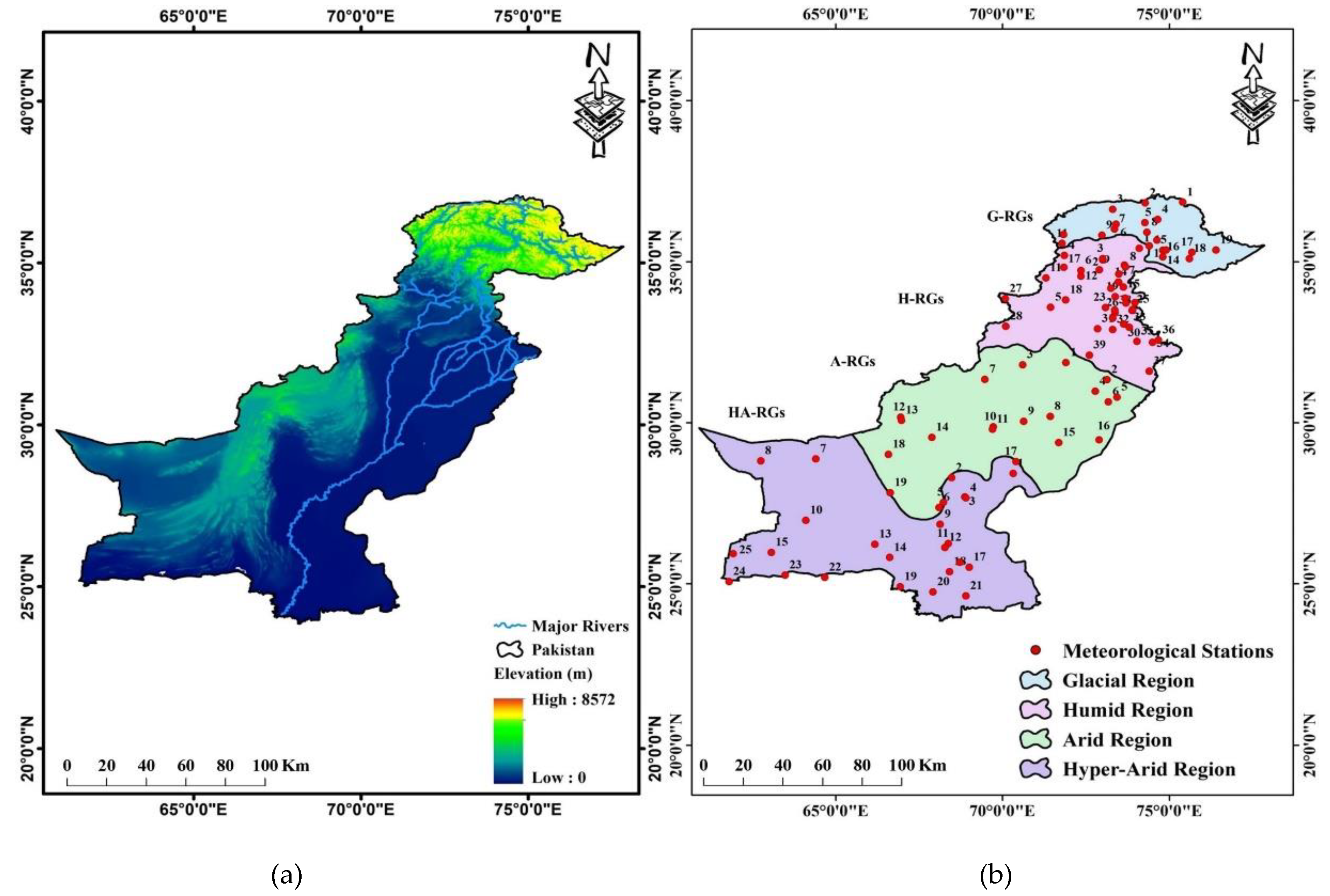
2.1. Study Area
2.2. In Situ Precipitation Data
2.3. Satellite Precipitation and Merged Satellite Precipitation Datasets (SPDs/MSPDs)
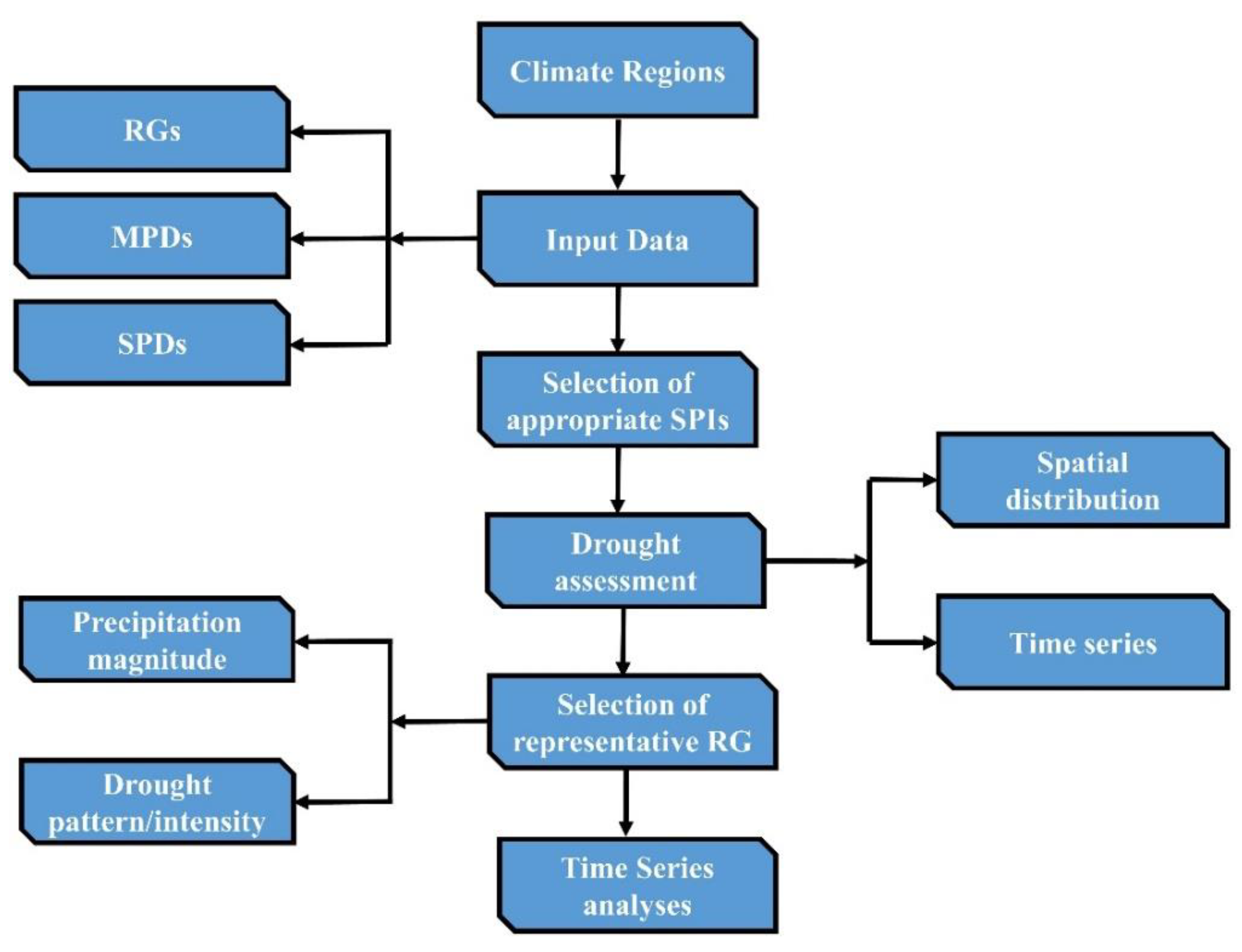
2.4. Methods
2.4.1. Standardized Precipitation Index (SPI)
2.4.2. Mann–Kendall (MK) Test
2.4.3. Sen’s Slope
2.4.4. Performance Evaluation of SPDs and MSPDs against the RGs in Drought Monitoring
3. Results
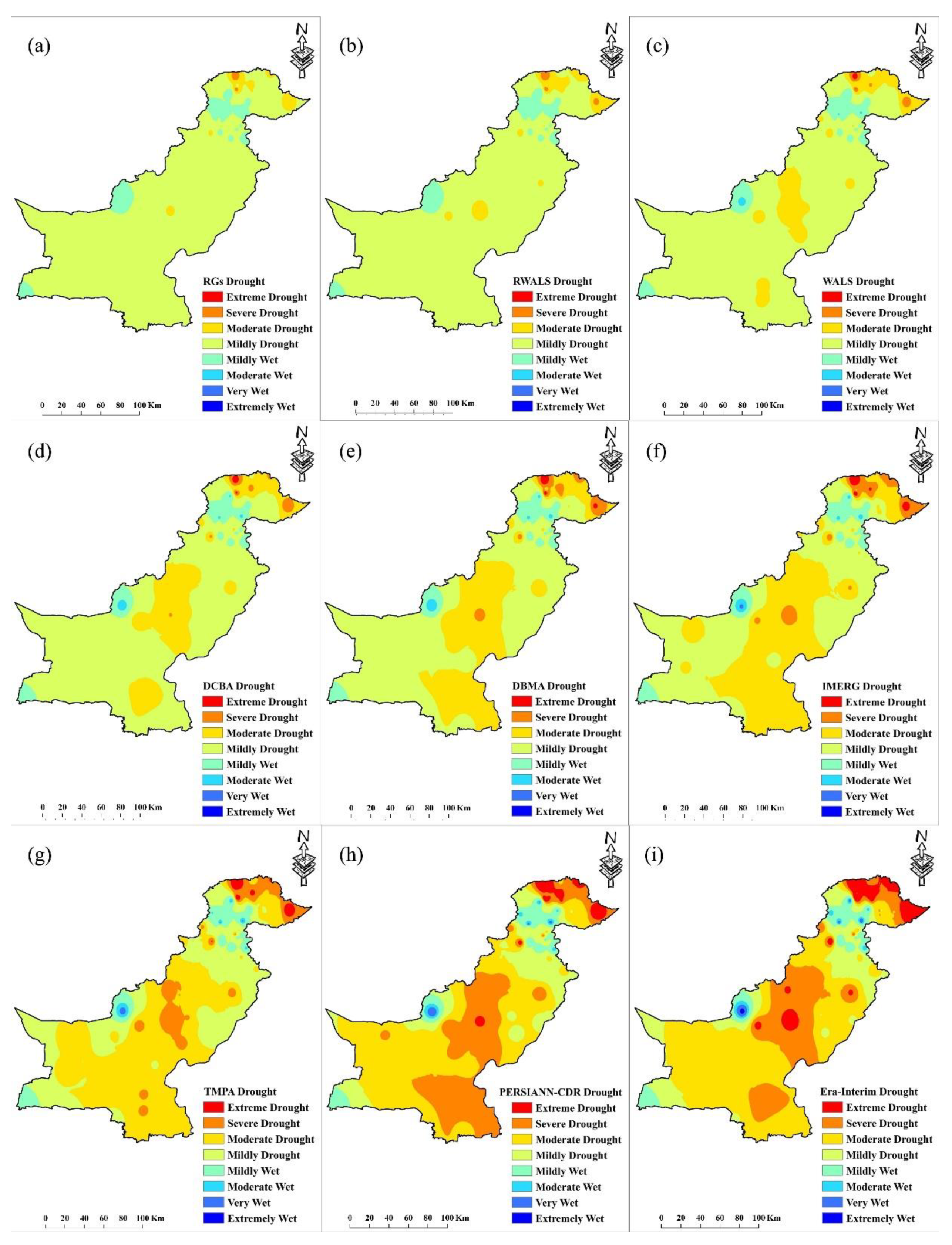
3.1. Performance of MSPDs and SPDs in Drought Assessment for a Representative Drought Year
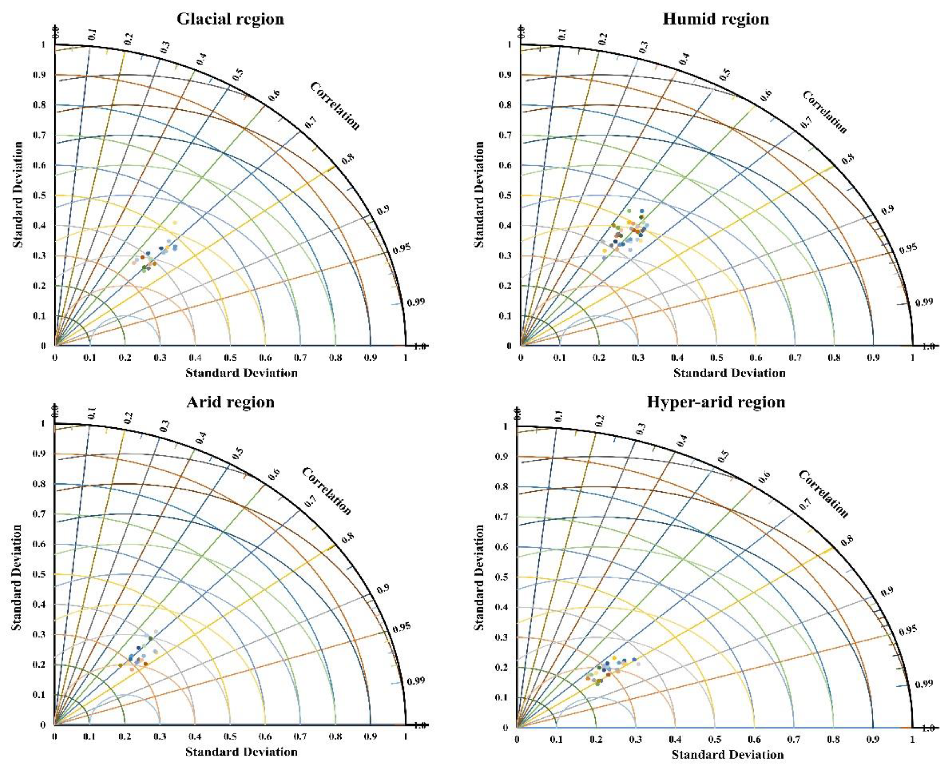
3.2. Regional-Scale Assessment of SPDs/MSPDs in Drought Monitoring
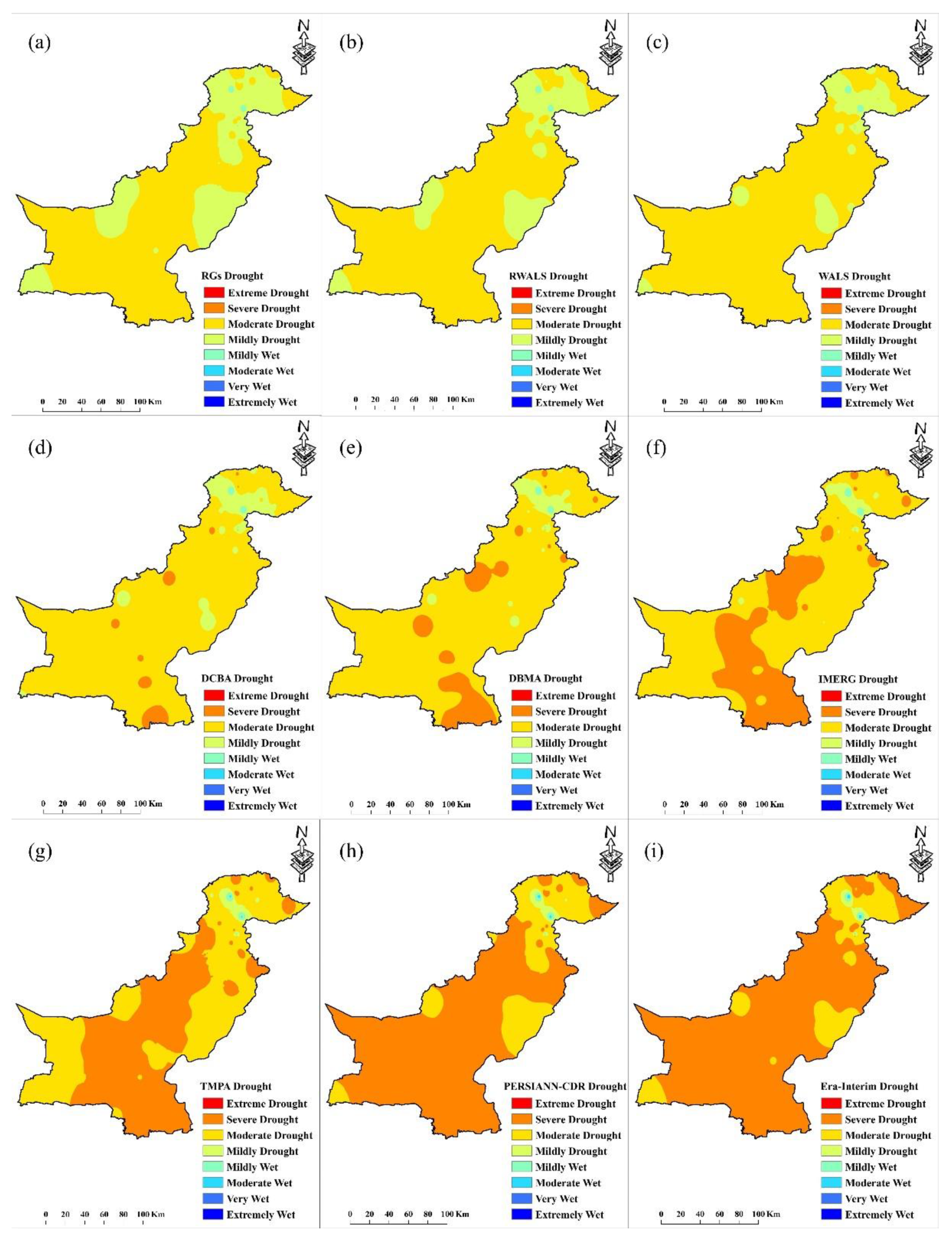
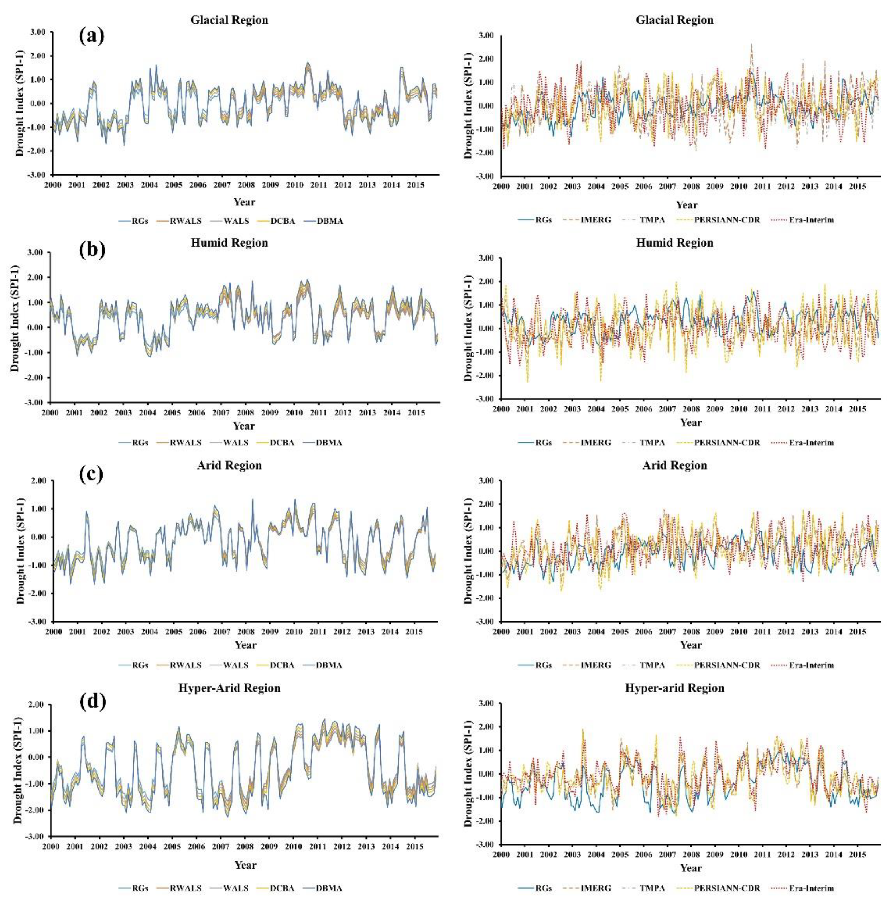
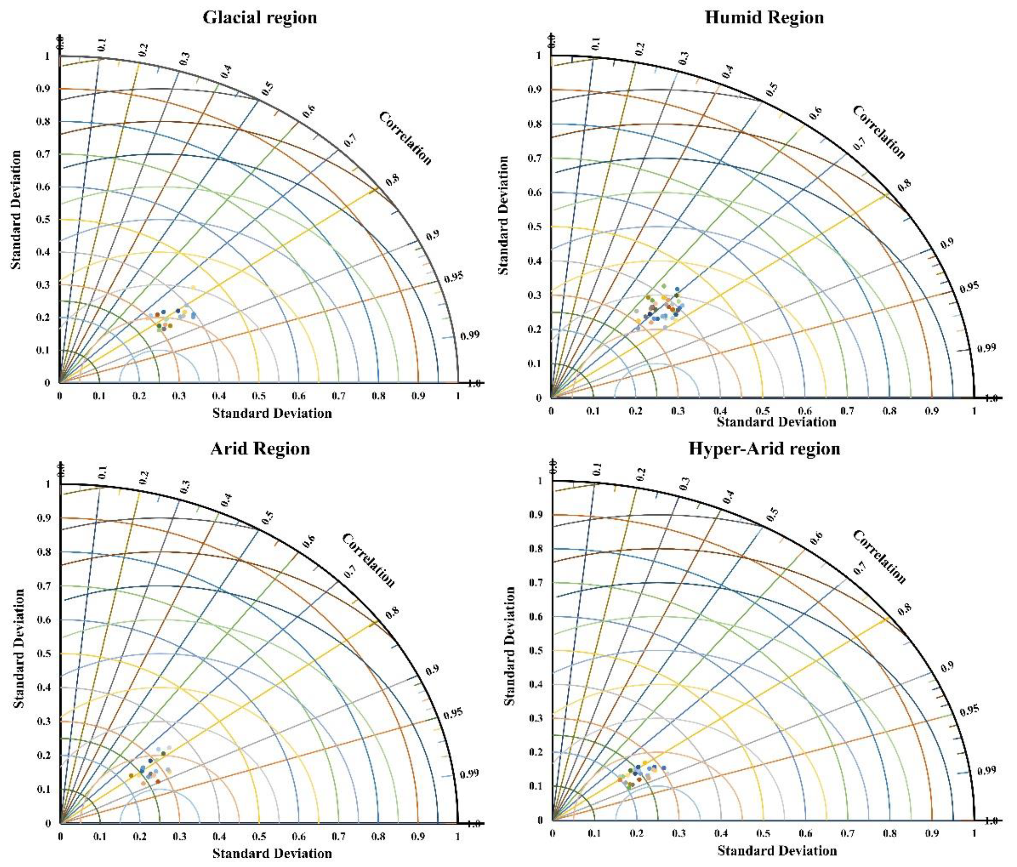
3.2.1. SPI-1
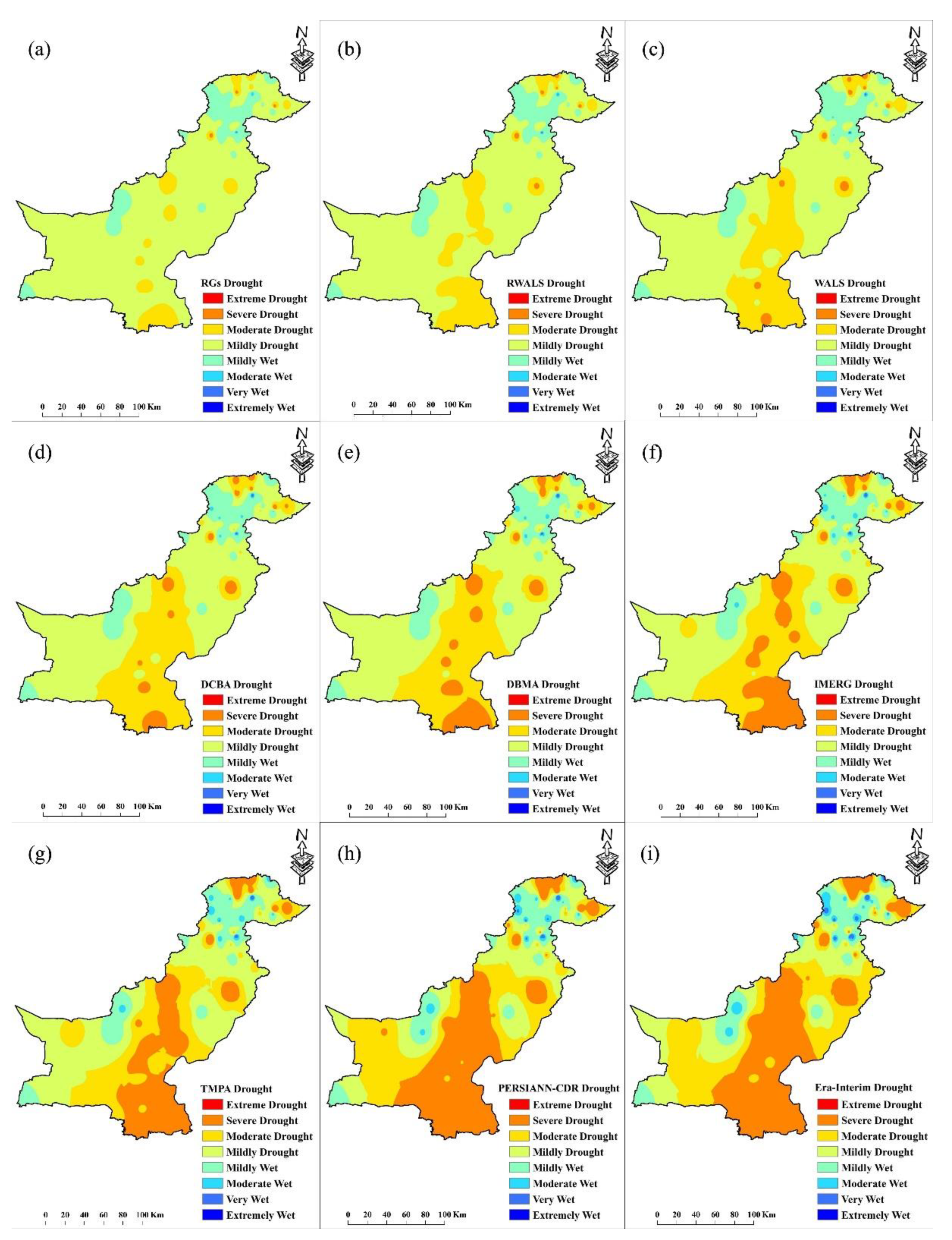
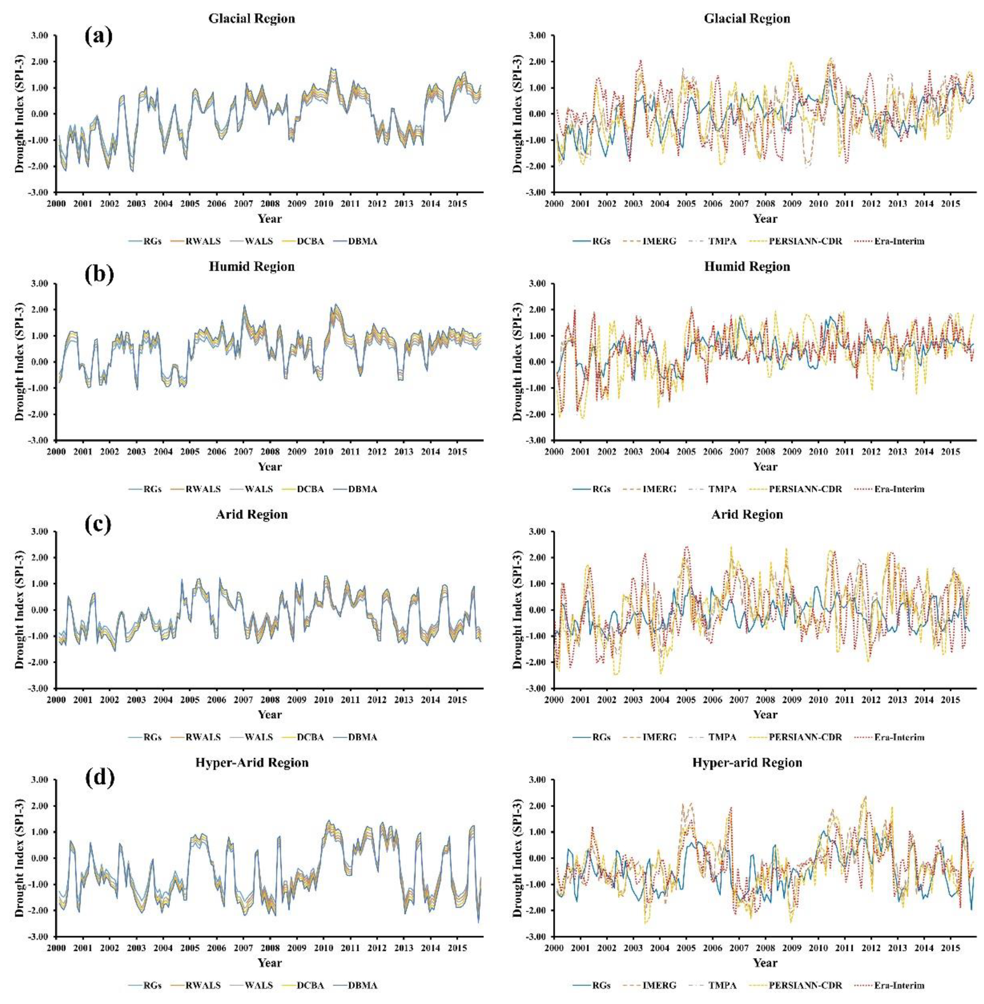
3.2.2. SPI-3
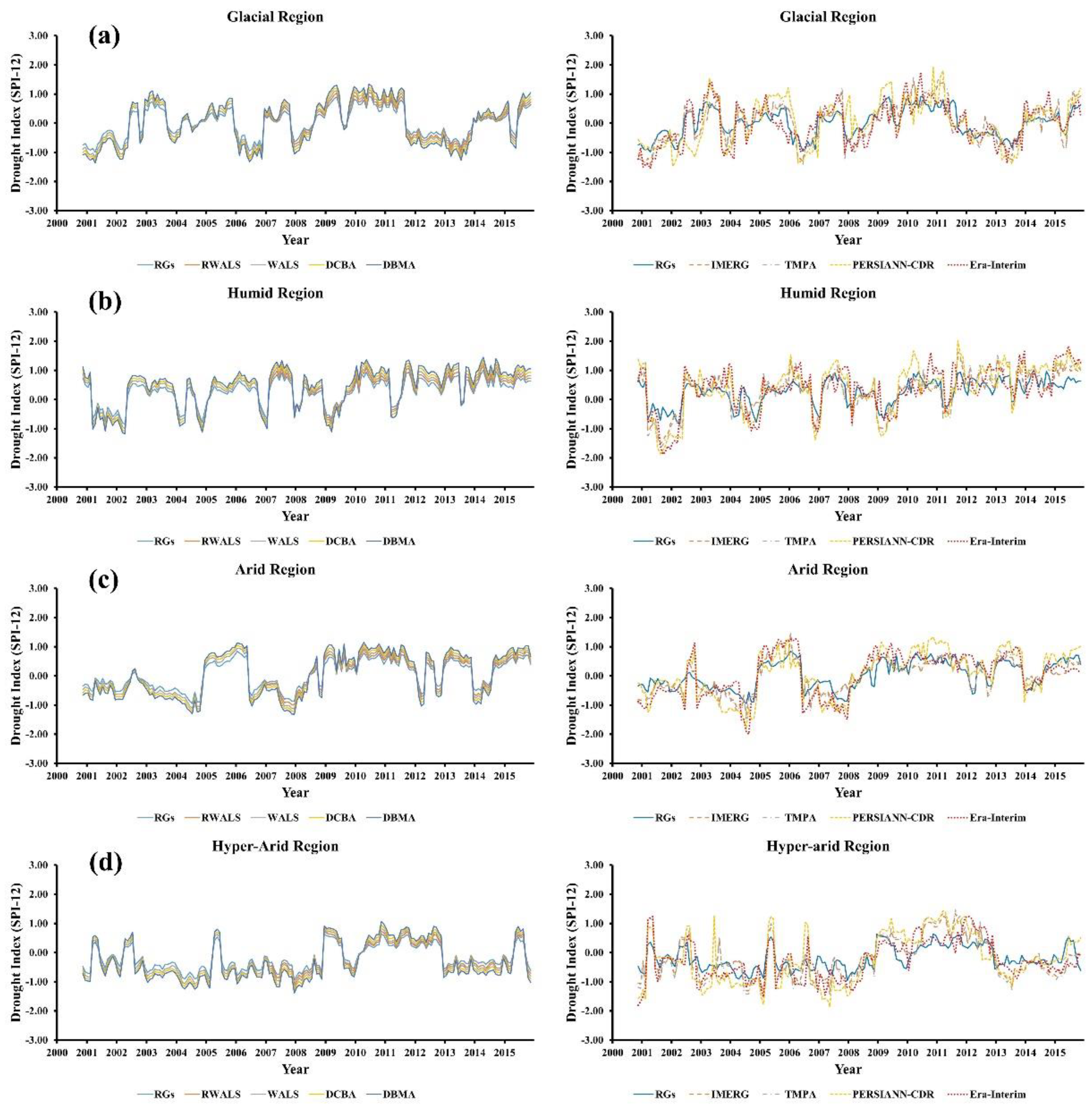
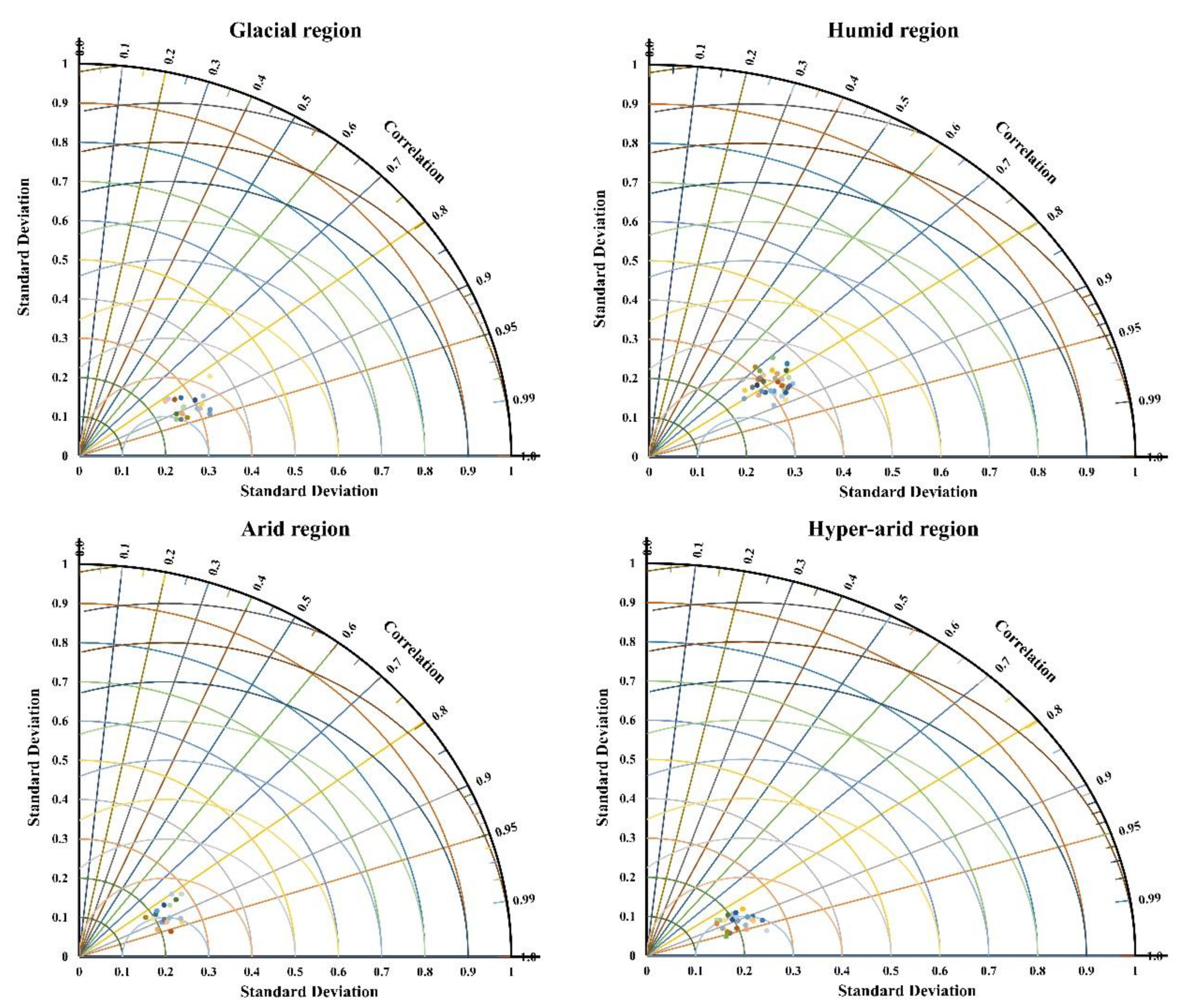
3.2.3. SPI-12
3.3. Trend Analyses of Drought Across Climate Regions of Pakistan
4. Discussion
4.1. Possible Data Sources of Precipitation and Their Limitations
4.2. Spatio-Temporal Pattern of Drought Across Pakistan
4.3. Comparison of Drought (SPI) with Different Time Scales
4.4. Potentials and Limitations of MSPDs
5. Conclusions
Author Contributions
Funding
Data Availability Statement
Acknowledgments
Conflicts of Interest
References
- Zarch, M.A.A.; Sivakumar, B.; Sharma, A. Droughts in a warming climate: A global assessment of Standardized precipitation index (SPI) and Reconnaissance drought index (RDI). J. Hydrol. 2015, 526, 183–195. [Google Scholar] [CrossRef]
- Sivakumar, B. Water crisis: From conflict to cooperation—An overview. Hydrol. Sci. J. 2011, 56, 531–552. [Google Scholar] [CrossRef]
- Haroon, M.A.; Zhang, J.; Yao, F. Drought monitoring and performance evaluation of MODIS-based drought severity index (DSI) over Pakistan. Nat. Hazards 2016, 84, 1349–1366. [Google Scholar] [CrossRef]
- Igbawua, T.; Zhang, J.; Yao, F.; Zhang, D. Assessment of moisture budget over West Africa using MERRA-2′s aerological model and satellite data. Clim. Dyn. 2019, 52, 83–106. [Google Scholar] [CrossRef]
- Yao, N.; Li, Y.; Lei, T.; Peng, L. Drought evolution, severity and trends in mainland China over 1961–2013. Sci. Total Environ. 2018, 616, 73–89. [Google Scholar] [CrossRef]
- Liu, Q.; Zhang, S.; Zhang, H.; Bai, Y.; Zhang, J. Monitoring drought using composite drought indices based on remote sensing. Sci. Total Environ. 2020, 711, 134585. [Google Scholar] [CrossRef]
- Kalisa, W.; Zhang, J.; Igbawua, T.; Ujoh, F.; Ebohon, O.J.; Namugize, J.N.; Yao, F. Spatio-temporal analysis of drought and return periods over the East African region using Standardized Precipitation Index from 1920 to 2016. Agric. Water Manag. 2020, 237, 106195. [Google Scholar] [CrossRef]
- Khan, N.; Sachindra, D.; Shahid, S.; Ahmed, K.; Shiru, M.S.; Nawaz, N. Prediction of droughts over Pakistan using machine learning algorithms. Adv. Water Resour. 2020, 139, 103562. [Google Scholar] [CrossRef]
- Xu, L.; Chen, N.; Zhang, X.; Chen, Z. An evaluation of statistical, NMME and hybrid models for drought prediction in China. J. Hydrol. 2018, 566, 235–249. [Google Scholar] [CrossRef]
- Gocic, M.; Trajkovic, S. Spatiotemporal characteristics of drought in Serbia. J. Hydrol. 2014, 510, 110–123. [Google Scholar] [CrossRef]
- Adnan, S.; Ullah, K.; Shuanglin, L.; Gao, S.; Khan, A.H.; Mahmood, R. Comparison of various drought indices to monitor drought status in Pakistan. Clim. Dyn. 2018, 51, 1885–1899. [Google Scholar] [CrossRef]
- Society, A.M. Meteorological drought-policy statement. Bull. Am. Meteorol. Soc. 1997, 78, 847–849. [Google Scholar]
- Shahid, M.; Rahman, K.U. Identifying the Annual and Seasonal Trends of Hydrological and Climatic Variables in the Indus Basin Pakistan. Asia Pac. J. Atmos. Sci. 2020, 57, 191–205. [Google Scholar] [CrossRef]
- Ahmed, K.; Shahid, S.; bin Harun, S.; Wang, X.-J. Characterization of seasonal droughts in Balochistan Province, Pakistan. Stoch. Environ. Res. Risk Assess. 2016, 30, 747–762. [Google Scholar] [CrossRef]
- Lin, A.; Wang, X.L. An algorithm for blending multiple satellite precipitation estimates with in situ precipitation measurements in Canada. J. Geophys. Res. Atmos. 2011, 116, D21111. [Google Scholar] [CrossRef]
- Lai, C.; Zhong, R.; Wang, Z.; Wu, X.; Chen, X.; Wang, P.; Lian, Y. Monitoring hydrological drought using long-term satellite-based precipitation data. Sci. Total Environ. 2019, 649, 1198–1208. [Google Scholar] [CrossRef] [PubMed]
- Zhong, R.; Chen, X.; Lai, C.; Wang, Z.; Lian, Y.; Yu, H.; Wu, X. Drought monitoring utility of satellite-based precipitation products across mainland China. J. Hydrol. 2019, 568, 343–359. [Google Scholar] [CrossRef]
- Rahman, K.U.; Shang, S.; Shahid, M.; Wen, Y.; Khan, Z. Application of a Dynamic Clustered Bayesian Model Averaging (DCBA) Algorithm for Merging Multisatellite Precipitation Products over Pakistan. J. Hydrometeorol. 2020, 21, 17–37. [Google Scholar] [CrossRef]
- Bai, X.; Wu, X.; Wang, P. Blending long-term satellite-based precipitation data with gauge observations for drought monitoring: Considering effects of different gauge densities. J. Hydrol. 2019, 577, 124007. [Google Scholar] [CrossRef]
- Dai, A. Increasing drought under global warming in observations and models. Nat. Clim. Chang. 2013, 3, 52–58. [Google Scholar] [CrossRef]
- IPCC. The Physical Science Basis of Climate Change; Cambridge University Press: Cambridge, UK, 2007. [Google Scholar]
- Wang, Z.; Zhong, R.; Lai, C.; Zeng, Z.; Lian, Y.; Bai, X. Climate change enhances the severity and variability of drought in the Pearl River Basin in South China in the 21st century. Agric. For. Meteorol. 2018, 249, 149–162. [Google Scholar] [CrossRef]
- Piao, S.; Ciais, P.; Huang, Y.; Shen, Z.; Peng, S.; Li, J.; Zhou, L.; Liu, H.; Ma, Y.; Ding, Y. The impacts of climate change on water resources and agriculture in China. Nature 2010, 467, 43–51. [Google Scholar] [CrossRef]
- Lai, C.; Li, J.; Wang, Z.; Wu, X.; Zeng, Z.; Chen, X.; Lian, Y.; Yu, H.; Wang, P.; Bai, X. Drought-induced reduction in net primary productivity across mainland China from 1982 to 2015. Remote Sens. 2018, 10, 1433. [Google Scholar] [CrossRef]
- Rahman, K.U.; Shang, S.; Shahid, M.; Wen, Y. Performance assessment of SM2RAIN-CCI and SM2RAIN-ASCAT precipitation products over Pakistan. Remote Sens. 2019, 11, 2040. [Google Scholar] [CrossRef]
- Baez-Villanueva, O.M.; Zambrano-Bigiarini, M.; Ribbe, L.; Nauditt, A.; Giraldo-Osorio, J.D.; Thinh, N.X. Temporal and spatial evaluation of satellite rainfall estimates over different regions in Latin-America. Atmos. Res. 2018, 213, 34–50. [Google Scholar] [CrossRef]
- Jin, B.; Wu, Y.; Miao, B.; Wang, X.L.; Guo, P. Bayesian spatiotemporal modeling for blending in situ observations with satellite precipitation estimates. J. Geophys. Res. Atmos. 2014, 119, 1806–1819. [Google Scholar] [CrossRef]
- Wang, Z.; Zhong, R.; Lai, C.; Chen, J. Evaluation of the GPM IMERG satellite-based precipitation products and the hydrological utility. Atmos. Res. 2017, 196, 151–163. [Google Scholar] [CrossRef]
- Sheffield, J.; Wood, E.F.; Roderick, M.L. Little change in global drought over the past 60 years. Nature 2012, 491, 435–438. [Google Scholar] [CrossRef] [PubMed]
- Trenberth, K.E.; Dai, A.; Van Der Schrier, G.; Jones, P.D.; Barichivich, J.; Briffa, K.R.; Sheffield, J. Global warming and changes in drought. Nat. Clim. Chang. 2014, 4, 17–22. [Google Scholar] [CrossRef]
- Sun, R.; Yuan, H.; Liu, X.; Jiang, X. Evaluation of the latest satellite–gauge precipitation products and their hydrologic applications over the Huaihe River basin. J. Hydrol. 2016, 536, 302–319. [Google Scholar] [CrossRef]
- Huffman, G.J.; Bolvin, D.T.; Nelkin, E.J.; Wolff, D.B.; Adler, R.F.; Gu, G.; Hong, Y.; Bowman, K.P.; Stocker, E.F. The TRMM multisatellite precipitation analysis (TMPA): Quasi-global, multiyear, combined-sensor precipitation estimates at fine scales. J. Hydrometeorol. 2007, 8, 38–55. [Google Scholar] [CrossRef]
- Mahmoud, M.T.; Al-Zahrani, M.A.; Sharif, H.O. Assessment of global precipitation measurement satellite products over Saudi Arabia. J. Hydrol. 2018, 559, 1–12. [Google Scholar] [CrossRef]
- Tang, G.; Wen, Y.; Gao, J.; Long, D.; Ma, Y.; Wan, W.; Hong, Y. Similarities and differences between three coexisting spaceborne radars in global rainfall and snowfall estimation. Water Resour. Res. 2017, 53, 3835–3853. [Google Scholar] [CrossRef]
- Hou, A.Y.; Kakar, R.K.; Neeck, S.; Azarbarzin, A.A.; Kummerow, C.D.; Kojima, M.; Oki, R.; Nakamura, K.; Iguchi, T. The global precipitation measurement mission. Bull. Am. Meteorol. Soc. 2014, 95, 701–722. [Google Scholar] [CrossRef]
- Hong, Y.; Hsu, K.-L.; Sorooshian, S.; Gao, X. Precipitation estimation from remotely sensed imagery using an artificial neural network cloud classification system. J. Appl. Meteorol. 2004, 43, 1834–1853. [Google Scholar] [CrossRef]
- Ashouri, H.; Hsu, K.-L.; Sorooshian, S.; Braithwaite, D.K.; Knapp, K.R.; Cecil, L.D.; Nelson, B.R.; Prat, O.P. PERSIANN-CDR: Daily precipitation climate data record from multisatellite observations for hydrological and climate studies. Bull. Am. Meteorol. Soc. 2015, 96, 69–83. [Google Scholar] [CrossRef]
- Joyce, R.J.; Janowiak, J.E.; Arkin, P.A.; Xie, P. CMORPH: A method that produces global precipitation estimates from passive microwave and infrared data at high spatial and temporal resolution. J. Hydrometeorol. 2004, 5, 487–503. [Google Scholar] [CrossRef]
- Dee, D.P.; Uppala, S.M.; Simmons, A.; Berrisford, P.; Poli, P.; Kobayashi, S.; Andrae, U.; Balmaseda, M.; Balsamo, G.; Bauer, D.P. The ERA—Interim reanalysis: Configuration and performance of the data assimilation system. Q. J. R. Meteorol. Soc. 2011, 137, 553–597. [Google Scholar] [CrossRef]
- Ma, Y.; Hong, Y.; Chen, Y.; Yang, Y.; Tang, G.; Yao, Y.; Long, D.; Li, C.; Han, Z.; Liu, R. Performance of optimally merged multisatellite precipitation products using the dynamic Bayesian model averaging scheme over the Tibetan Plateau. J. Geophys. Res. Atmos. 2018, 123, 814–834. [Google Scholar] [CrossRef]
- Rahman, K.U.; Shang, S.; Shahid, M.; Li, J. Developing an ensemble precipitation algorithm from satellite products and its topographical and seasonal evaluations over Pakistan. Remote Sens. 2018, 10, 1835. [Google Scholar] [CrossRef]
- Tang, G.; Ma, Y.; Long, D.; Zhong, L.; Hong, Y. Evaluation of GPM Day-1 IMERG and TMPA Version-7 legacy products over Mainland China at multiple spatiotemporal scales. J. Hydrol. 2016, 533, 152–167. [Google Scholar] [CrossRef]
- Wang, L.; Li, X.; Ma, C.; Bai, Y. Improving the prediction accuracy of monthly streamflow using a data-driven model based on a double-processing strategy. J. Hydrol. 2019, 573, 733–745. [Google Scholar] [CrossRef]
- Lin, P.; Pan, M.; Allen, G.H.; de Frasson, R.P.; Zeng, Z.; Yamazaki, D.; Wood, E.F. Global estimates of reach—Level bankfull river width leveraging big data geospatial analysis. Geophys. Res. Lett. 2020, 47, e2019GL086405. [Google Scholar] [CrossRef]
- Derin, Y.; Bhuiyan, M.A.E.; Anagnostou, E.; Kalogiros, J.; Anagnostou, M.N. Modeling Level 2 Passive Microwave Precipitation Retrieval Error Over Complex Terrain Using a Nonparametric Statistical Technique. IEEE Trans. Geosci. Remote Sens. 2021, in press. [Google Scholar] [CrossRef]
- Bhuiyan, M.A.E.; Yang, F.; Biswas, N.K.; Rahat, S.H.; Neelam, T.J. Machine learning-based error modeling to improve GPM IMERG precipitation product over the brahmaputra river basin. Forecasting 2020, 2, 14. [Google Scholar] [CrossRef]
- Kumar, A.; Ramsankaran, R.; Brocca, L.; Munoz-Arriola, F. A Machine Learning Approach for Improving Near-Real-Time Satellite-Based Rainfall Estimates by Integrating Soil Moisture. Remote Sens. 2019, 11, 2221. [Google Scholar] [CrossRef]
- Zhang, L.; Li, X.; Zheng, D.; Zhang, K.; Ma, Q.; Zhao, Y.; Ge, Y. Merging multiple satellite-based precipitation products and gauge observations using a novel double machine learning approach. J. Hydrol. 2021, 594, 125969. [Google Scholar] [CrossRef]
- Bhuiyan, M.A.E.; Nikolopoulos, E.I.; Anagnostou, E.N.; Quintana-Seguí, P.; Barella-Ortiz, A. A nonparametric statistical technique for combining global precipitation datasets: Development and hydrological evaluation over the Iberian Peninsula. Hydrol. Earth Syst. Sci. 2018, 22, 1371–1389. [Google Scholar] [CrossRef]
- Baez-Villanueva, O.M.; Zambrano-Bigiarini, M.; Beck, H.E.; McNamara, I.; Ribbe, L.; Nauditt, A.; Birkel, C.; Verbist, K.; Giraldo-Osorio, J.D.; Thinh, N.X. RF-MEP: A novel Random Forest method for merging gridded precipitation products and ground-based measurements. Remote Sens. Environ. 2020, 239, 111606. [Google Scholar] [CrossRef]
- Wehbe, Y.; Temimi, M.; Adler, R.F. Enhancing precipitation estimates through the fusion of weather radar, satellite retrievals, and surface parameters. Remote Sens. 2020, 12, 1342. [Google Scholar] [CrossRef]
- Wu, H.; Yang, Q.; Liu, J.; Wang, G. A spatiotemporal deep fusion model for merging satellite and gauge precipitation in China. J. Hydrol. 2020, 584, 124664. [Google Scholar] [CrossRef]
- Yin, J.; Guo, S.; Gu, L.; Zeng, Z.; Liu, D.; Chen, J.; Shen, Y.; Xu, C.-Y. Blending multi-satellite, atmospheric reanalysis and gauge precipitation products to facilitate hydrological modelling. J. Hydrol. 2021, 593, 125878. [Google Scholar] [CrossRef]
- Rahman, K.U.; Shang, S.; Shahid, M.; Wen, Y. An Appraisal of Dynamic Bayesian Model Averaging-based Merged Multi-Satellite Precipitation Datasets Over Complex Topography and the Diverse Climate of Pakistan. Remote Sens. 2020, 12, 10. [Google Scholar] [CrossRef]
- Rahman, K.U.; Shang, S.; Shahid, M.; Wen, Y.; Khan, A.J. Development of a novel weighted average least squares-based ensemble multi-satellite precipitation dataset and its comprehensive evaluation over Pakistan. Atmos. Res. 2020, 246, 105133. [Google Scholar] [CrossRef]
- Rahman, K.U.; Shang, S.; Rahman, K.U.; Shang, S. A Regional Blended Precipitation Dataset over Pakistan Based on Regional Selection of Blending Satellite Precipitation Datasets and the Dynamic Weighted Average Least Squares Algorithm. Remote Sens. 2020, 12, 4009. [Google Scholar] [CrossRef]
- Rahman, K.U.; Shang, S.; Shahid, M.; Wen, Y. Hydrological evaluation of merged satellite precipitation datasets for streamflow simulation using SWAT: A case study of Potohar Plateau, Pakistan. J. Hydrol. 2020, 587, 125040. [Google Scholar] [CrossRef]
- Ma, Y.; Yang, Y.; Han, Z.; Tang, G.; Maguire, L.; Chu, Z.; Hong, Y. Comprehensive evaluation of ensemble multi-satellite precipitation dataset using the dynamic bayesian model averaging scheme over the Tibetan Plateau. J. Hydrol. 2018, 556, 634–644. [Google Scholar] [CrossRef]
- Yong, B.; Ren, L.L.; Hong, Y.; Wang, J.H.; Gourley, J.J.; Jiang, S.H.; Chen, X.; Wang, W. Hydrologic evaluation of Multisatellite Precipitation Analysis standard precipitation products in basins beyond its inclined latitude band: A case study in Laohahe basin, China. Water Resour. Res. 2010, 46, W07542. [Google Scholar] [CrossRef]
- Sahoo, A.K.; Sheffield, J.; Pan, M.; Wood, E.F. Evaluation of the tropical rainfall measuring mission multi-satellite precipitation analysis (TMPA) for assessment of large-scale meteorological drought. Remote Sens. Environ. 2015, 159, 181–193. [Google Scholar] [CrossRef]
- Duan, Z.; Liu, J.; Tuo, Y.; Chiogna, G.; Disse, M. Evaluation of eight high spatial resolution gridded precipitation products in Adige Basin (Italy) at multiple temporal and spatial scales. Sci. Total Environ. 2016, 573, 1536–1553. [Google Scholar] [CrossRef]
- Katsanos, D.; Retalis, A.; Michaelides, S. Validation of a high-resolution precipitation database (CHIRPS) over Cyprus for a 30-year period. Atmos. Res. 2016, 169, 459–464. [Google Scholar] [CrossRef]
- Zambrano, F.; Wardlow, B.; Tadesse, T.; Lillo-Saavedra, M.; Lagos, O. Evaluating satellite-derived long-term historical precipitation datasets for drought monitoring in Chile. Atmos. Res. 2017, 186, 26–42. [Google Scholar] [CrossRef]
- Gao, F.; Zhang, Y.; Chen, Q.; Wang, P.; Yang, H.; Yao, Y.; Cai, W. Comparison of two long-term and high-resolution satellite precipitation datasets in Xinjiang, China. Atmos. Res. 2018, 212, 150–157. [Google Scholar] [CrossRef]
- Guo, H.; Bao, A.; Liu, T.; Chen, S.; Ndayisaba, F. Evaluation of PERSIANN-CDR for meteorological drought monitoring over China. Remote Sens. 2016, 8, 379. [Google Scholar] [CrossRef]
- Hanif, M.; Khan, A.H.; Adnan, S. Latitudinal precipitation characteristics and trends in Pakistan. J. Hydrol. 2013, 492, 266–272. [Google Scholar] [CrossRef]
- Asmat, U.; Athar, H. Run-based multi-model interannual variability assessment of precipitation and temperature over Pakistan using two IPCC AR4-based AOGCMs. Theor. Appl. Climatol. 2017, 127, 1–16. [Google Scholar] [CrossRef]
- Balkhair, K.S.; Rahman, K.U. Sustainable and economical small-scale and low-head hydropower generation: A promising alternative potential solution for energy generation at local and regional scale. Appl. Energy 2017, 188, 378–391. [Google Scholar] [CrossRef]
- Hussain, Y.; Satgé, F.; Hussain, M.B.; Martinez-Carvajal, H.; Bonnet, M.-P.; Cárdenas-Soto, M.; Roig, H.L.; Akhter, G. Performance of CMORPH, TMPA, and PERSIANN rainfall datasets over plain, mountainous, and glacial regions of Pakistan. Theor. Appl. Climatol. 2018, 131, 1119–1132. [Google Scholar] [CrossRef]
- Iqbal, M.F.; Athar, H. Validation of satellite based precipitation over diverse topography of Pakistan. Atmos. Res. 2018, 201, 247–260. [Google Scholar] [CrossRef]
- Khan, N.; Shahid, S.; bin Ismail, T.; Wang, X.-J. Spatial distribution of unidirectional trends in temperature and temperature extremes in Pakistan. Theor. Appl. Climatol. 2019, 136, 899–913. [Google Scholar] [CrossRef]
- Kumar, K.K.; Rajagopalan, B.; Cane, M.A. On the weakening relationship between the Indian monsoon and ENSO. Science 1999, 284, 2156–2159. [Google Scholar] [CrossRef] [PubMed]
- Hunt, K.M.; Turner, A.G.; Shaffrey, L.C. The evolution, seasonality and impacts of western disturbances. Q. J. R. Meteorol. Soc. 2018, 144, 278–290. [Google Scholar] [CrossRef]
- Ahmed, K.; Shahid, S.; Nawaz, N. Impacts of climate variability and change on seasonal drought characteristics of Pakistan. Atmos. Res. 2018, 214, 364–374. [Google Scholar] [CrossRef]
- Dimri, A.; Niyogi, D.; Barros, A.; Ridley, J.; Mohanty, U.; Yasunari, T.; Sikka, D. Western disturbances: A review. Rev. Geophys. 2015, 53, 225–246. [Google Scholar] [CrossRef]
- Huffman, G.J.; Bolvin, D.T.; Braithwaite, D.; Hsu, K.; Joyce, R.; Kidd, C.; Nelkin, E.J.; Sorooshian, S.; Tan, J.; Xie, P. NASA Global Precipitation Measurement (GPM). In Integrated Multi-Satellite Retrievals for GPM (IMERG), Algorithm Theoretical Basis Document (ATBD) Version 5.2; NASA/GSFC: Greenbelt, MD, USA, 2018. [Google Scholar]
- Brocca, L.; Ciabatta, L.; Massari, C.; Moramarco, T.; Hahn, S.; Hasenauer, S.; Kidd, R.; Dorigo, W.; Wagner, W.; Levizzani, V. Soil as a natural rain gauge: Estimating global rainfall from satellite soil moisture data. J. Geophys. Res. Atmos. 2014, 119, 5128–5141. [Google Scholar] [CrossRef]
- Brocca, L.; Filippucci, P.; Hahn, S.; Ciabatta, L.; Massari, C.; Camici, S.; Schüller, L.; Bojkov, B.; Wagner, W. SM2RAIN-ASCAT (2007–2018): Global daily satellite rainfall from ASCAT soil moisture. Earth Syst. Sci. Data 2019, 11, 1583–1601. [Google Scholar] [CrossRef]
- Brocca, L.; Moramarco, T.; Melone, F.; Wagner, W. A new method for rainfall estimation through soil moisture observations. Geophys. Res. Lett. 2013, 40, 853–858. [Google Scholar] [CrossRef]
- Ciabatta, L.; Massari, C.; Brocca, L.; Gruber, A.; Reimer, C.; Hahn, S.; Paulik, C.; Dorigo, W.; Kidd, R.; Wagner, W. SM2RAIN-CCI: A new global long-term rainfall data set derived from ESA CCI soil moisture. Earth Syst. Sci. Data 2018, 10, 267. [Google Scholar] [CrossRef]
- Farahmand, A.; AghaKouchak, A. A generalized framework for deriving nonparametric standardized drought indicators. Adv. Water Resour. 2015, 76, 140–145. [Google Scholar] [CrossRef]
- McKee, T.B.; Doesken, N.J.; Kleist, J. The relationship of drought frequency and duration to time scales. In Proceedings of the 8th Conference on Applied Climatology, Anaheim, CA, USA, 17–22 January 1993; pp. 179–183. [Google Scholar]
- Mann, H.B. Nonparametric tests against trend. Econom. J. Econom. Soc. 1945, 13, 245–259. [Google Scholar] [CrossRef]
- Kendall, M.G. Rank Correlation Methods; Charles Griffin and Co. Ltd.: London, UK, 1948. [Google Scholar]
- Fu, G.; Chen, S.; Liu, C.; Shepard, D. Hydro-climatic trends of the Yellow River basin for the last 50 years. Clim. Chang. 2004, 65, 149–178. [Google Scholar] [CrossRef]
- Sen, P.K. Estimates of the regression coefficient based on Kendall’s tau. J. Am. Stat. Assoc. 1968, 63, 1379–1389. [Google Scholar] [CrossRef]
- West, K.D. Forecast evaluation. In Handbook of Economic Forecasting; Elsevier: Amsterdam, The Netherlands, 2006; Volume 1, pp. 99–134. [Google Scholar]
- Lewis, C.D. Industrial and Business Forecasting Methods: A Practical Guide to Exponential Smoothing and Curve Fitting; Butterworth-Heinemann: Oxford, UK, 1982. [Google Scholar]
- Tapiador, F.; Navarro, A.; Levizzani, V.; García-Ortega, E.; Huffman, G.; Kidd, C.; Kucera, P.; Kummerow, C.; Masunaga, H.; Petersen, W. Global precipitation measurements for validating climate models. Atmos. Res. 2017, 197, 1–20. [Google Scholar] [CrossRef]
- Mastrantonas, N.; Bhattacharya, B.; Shibuo, Y.; Rasmy, M.; Espinoza-Dávalos, G.; Solomatine, D. Evaluating the benefits of merging near-real-time satellite precipitation products: A case study in the Kinu basin region, Japan. J. Hydrometeorol. 2019, 20, 1213–1233. [Google Scholar] [CrossRef]
- Ma, Y.; Sun, X.; Chen, H.; Hong, Y.; Zhang, Y. A two-stage blending approach for merging multiple satellite precipitation estimates and rain gauge observations: An experiment in the northeastern Tibetan Plateau. Hydrol. Earth Syst. Sci. 2021, 25, 359–374. [Google Scholar] [CrossRef]
- Belo-Pereira, M.; Dutra, E.; Viterbo, P. Evaluation of global precipitation data sets over the Iberian Peninsula. J. Geophys. Res. 2011, 116, D20101. [Google Scholar] [CrossRef]
- Thiemig, V.; Rojas, R.; Zambrano-Bigiarini, M.; Levizzani, V.; De Roo, A. Validation of satellite-based precipitation products over sparsely gauged African river basins. J. Hydrometeorol. 2012, 13, 1760–1783. [Google Scholar] [CrossRef]
- Naud, C.M.; Booth, J.F.; Del Genio, A.D. Evaluation of ERA-Interim and MERRA cloudiness in the Southern Ocean. J. Clim. 2014, 27, 2109–2124. [Google Scholar] [CrossRef]
- Dinku, T.; Connor, S.J.; Ceccato, P. Comparison of CMORPH and TRMM-3B42 over mountainous regions of Africa and South America. In Satellite Rainfall Applications for Surface Hydrology; Springer: Dordrecht, The Netherlands, 2010; pp. 193–204. [Google Scholar]
- Hong, Y.; Gochis, D.; Cheng, J.T.; Hsu, K.L.; Sorooshian, S. Evaluation of PERSIANN-CCS rainfall measurement using the NAME event rain gauge network. J. Hydrometeorol. 2007, 8, 469–482. [Google Scholar] [CrossRef]
- Bitew, M.M.; Gebremichael, M. Evaluation through independent measurements: Complex terrain and humid tropical region in Ethiopia. In Satellite Rainfall Applications for Surface Hydrology; Springer: Dordrecht, The Netherlands, 2010; pp. 205–214. [Google Scholar]
- Villarini, G.; Krajewski, W.F. Review of the different sources of uncertainty in single polarization radar-based estimates of rainfall. Surv. Geophys. 2010, 31, 107–129. [Google Scholar] [CrossRef]
- AghaKouchak, A.; Nasrollahi, N.; Habib, E. Accounting for uncertainties of the TRMM satellite estimates. Remote Sens. 2009, 1, 606–619. [Google Scholar] [CrossRef]
- Scheel, M.L.M.; Rohrer, M.; Huggel, C.; Santos Villar, D.; Silvestre, E.; Huffman, G.J. Evaluation of TRMM Multi-satellite Precipitation Analysis (TMPA) performance in the Central Andes region and its dependency on spatial and temporal resolution. Hydrol. Earth Syst. Sci. 2011, 15, 2649–2663. [Google Scholar] [CrossRef]
- Zhang, L.; Li, X.; Cao, Y.; Nan, Z.; Wang, W.; Ge, Y.; Yu, W. Evaluation and integration of the top-down and bottom-up satellite precipitation products over mainland China. J. Hydrol. 2020, 581, 124456. [Google Scholar] [CrossRef]
- Sharifi, E.; Saghafian, B.; Steinacker, R. Downscaling satellite precipitation estimates with multiple linear regression, artificial neural networks, and spline interpolation techniques. J. Geophys. Res. Atmos. 2019, 124, 789–805. [Google Scholar] [CrossRef]


| SPD/MSPD | Spatial Resolution | Temporal Span | Temporal Resolution | Retrieval/Merging Algorithm | References |
|---|---|---|---|---|---|
| IMERG V06 | 0.10° | 2000–2015 | 1-day | Goddard profiling algorithm | [76] |
| TMPA 3B42 V7 | 0.25° | 2000–2015 | 1-day | GPCC monthly gauge observation to correct the bias of 3B42RT | [32] |
| Era-Interim | 0.25° | 2000–2015 | 1-day | 4D-Var analysis | [39] |
| PERSIANN-CDR | 0.25° | 2000–2015 | 1-day | Adaptive artificial neural network | [37] |
| DBMA-MSPD | 0.25° | 2000–2015 | 1-day | Dynamic Bayesian Model Averaging (DBMA) | [54] |
| DCBA-MSPD | 0.25° | 2000–2015 | 1-day | Dynamic Clustered Bayesian Model Averaging (DCBA) | [18] |
| WALS-MSPD | 0.25° | 2000–2015 | 1-day | Dynamic Weighted Average Least Square (WALS) | [55] |
| RWALS-MSP | 0.25° | 2007–2018 | 1-day | Dynamic Regional Weighted Average Least Square (RWALS) | [56] |
| MSPDs | No. | Climate Regions | |||
|---|---|---|---|---|---|
| Glacial | Humid | Arid | Hyper-Arid | ||
| RWALS | 1 | IMERG V06 | IMERG V06 | IMERG V06 | IMERG V06 |
| 2 | TMPA 3B42 V7 | TMPA 3B42 V7 | TMPA 3B42 V7 | SM2RIAN-ASCAT | |
| 3 | SM2RAIN-ASCAT | SM2RAIN-ASCAT | SM2RAIN-ASCAT | SM2RAIN-CCI | |
| 4 | PERSIANN-CDR | SM2RAIN-CCI | SM2RAIN-CCI | Era-Interim | |
| WALS | 1–4 | TMPA 3B42 V7, PERSIANN-CDR, ERA-Interim, and CMORPH | |||
| DCBA | 1–4 | TMPA 3B42 V7, PERSIANN-CDR, ERA-Interim, and CMORPH | |||
| DBMA | 1–4 | TMPA 3B42 V7, PERSIANN-CDR, ERA-Interim, and CMORPH | |||
| SPI Range | Description |
|---|---|
| >2 | Extremely wet |
| 1.5 to 1.99 | Very wet |
| 1.0 to 1.49 | Moderately wet |
| 0 to 1.0 | Mildly wet |
| −1.0 to 0 | Mildly drought |
| −1.5 to −1.0 | Moderately drought |
| −2.0 to −1.5 | Severe drought |
| <−2 | Extreme drought |
| Climate Region | SPDs/MSPDs | MAD | RMSD | MAPD |
|---|---|---|---|---|
| Glacial | RAWALS | 0.683 | 0.972 | 9.311 |
| WALS | 0.853 | 1.157 | 12.365 | |
| DCBA | 1.059 | 1.268 | 19.532 | |
| DBMA | 1.362 | 1.453 | 27.789 | |
| IMERG | 1.439 | 1.632 | 33.985 | |
| TMPA | 1.748 | 1.722 | 39.108 | |
| PERSIANN-CDR | 1.951 | 1.738 | 44.761 | |
| Era-Interim | 2.011 | 1.931 | 47.316 | |
| Humid | RAWALS | 1.038 | 1.117 | 8.186 |
| WALS | 1.158 | 1.258 | 13.586 | |
| DCBA | 1.559 | 1.371 | 21.592 | |
| DBMA | 1.695 | 1.577 | 25.623 | |
| IMERG | 2.018 | 1.675 | 32.771 | |
| TMPA | 2.365 | 1.768 | 37.195 | |
| PERSIANN-CDR | 2.531 | 1.796 | 43.257 | |
| Era-Interim | 2.644 | 1.956 | 47.974 | |
| Arid | RAWALS | 0.569 | 0.891 | 7.126 |
| WALS | 0.648 | 0.921 | 10.012 | |
| DCBA | 0.707 | 1.147 | 16.353 | |
| DBMA | 0.873 | 1.246 | 21.797 | |
| IMERG | 0.985 | 1.344 | 27.829 | |
| TMPA | 1.361 | 1.497 | 32.179 | |
| PERSIANN-CDR | 1.733 | 1.558 | 40.944 | |
| Era-Interim | 1.887 | 1.672 | 42.687 | |
| Hyper-arid | RAWALS | 0.238 | 0.816 | 5.131 |
| WALS | 0.583 | 0.895 | 8.680 | |
| DCBA | 0.730 | 0.985 | 12.004 | |
| DBMA | 0.832 | 1.048 | 17.561 | |
| IMERG | 0.879 | 1.218 | 21.013 | |
| TMPA | 1.135 | 1.332 | 24.392 | |
| PERSIANN-CDR | 1.495 | 1.478 | 32.504 | |
| Era-Interim | 1.363 | 1.652 | 29.853 |
| Climate Region | SPDs/MSPDs | MAD | RMSD | MAPD |
|---|---|---|---|---|
| Glacial | RAWALS | 0.592 | 0.897 | 9.205 |
| WALS | 0.794 | 1.022 | 13.718 | |
| DCBA | 0.966 | 1.193 | 19.887 | |
| DBMA | 1.241 | 1.318 | 25.043 | |
| IMERG | 1.388 | 1.446 | 31.191 | |
| TMPA | 1.623 | 1.566 | 37.411 | |
| PERSIANN-CDR | 1.875 | 1.656 | 43.526 | |
| Era-Interim | 1.976 | 1.746 | 48.667 | |
| Humid | RAWALS | 0.942 | 1.102 | 9.066 |
| WALS | 1.074 | 1.181 | 12.988 | |
| DCBA | 1.410 | 1.272 | 19.700 | |
| DBMA | 1.640 | 1.468 | 24.352 | |
| IMERG | 1.924 | 1.520 | 31.019 | |
| TMPA | 2.229 | 1.622 | 35.793 | |
| PERSIANN-CDR | 2.439 | 1.705 | 41.383 | |
| Era-Interim | 2.561 | 1.799 | 44.287 | |
| Arid | RAWALS | 0.485 | 0.873 | 8.107 |
| WALS | 0.554 | 0.903 | 9.585 | |
| DCBA | 0.671 | 1.034 | 15.824 | |
| DBMA | 0.844 | 1.142 | 20.171 | |
| IMERG | 1.148 | 1.237 | 25.908 | |
| TMPA | 1.280 | 1.384 | 31.483 | |
| PERSIANN-CDR | 1.639 | 1.454 | 39.172 | |
| Era-Interim | 1.705 | 1.597 | 43.187 | |
| Hyper-arid | RAWALS | 0.209 | 0.761 | 6.394 |
| WALS | 0.484 | 0.790 | 9.569 | |
| DCBA | 0.602 | 0.859 | 11.861 | |
| DBMA | 0.813 | 0.990 | 16.503 | |
| IMERG | 0.837 | 1.125 | 19.897 | |
| TMPA | 1.063 | 1.219 | 22.962 | |
| PERSIANN-CDR | 1.386 | 1.400 | 29.878 | |
| Era-Interim | 1.296 | 1.322 | 28.974 |
| Climate Region | SPDs/MSPDs | MAD | RMSD | MAPD |
|---|---|---|---|---|
| Glacial | RAWALS | 0.378 | 0.680 | 6.713 |
| WALS | 0.467 | 0.851 | 9.479 | |
| DCBA | 0.670 | 0.942 | 13.496 | |
| DBMA | 0.859 | 1.132 | 18.786 | |
| IMERG | 0.977 | 1.244 | 23.448 | |
| TMPA | 1.206 | 1.353 | 29.732 | |
| PERSIANN-CDR | 1.399 | 1.452 | 34.562 | |
| Era-Interim | 1.698 | 1.579 | 38.882 | |
| Humid | RAWALS | 0.607 | 0.892 | 5.309 |
| WALS | 0.815 | 0.916 | 8.085 | |
| DCBA | 0.942 | 1.152 | 13.096 | |
| DBMA | 1.253 | 1.304 | 17.506 | |
| IMERG | 1.574 | 1.406 | 23.814 | |
| TMPA | 1.803 | 1.455 | 28.744 | |
| PERSIANN-CDR | 1.866 | 1.579 | 34.592 | |
| Era-Interim | 2.179 | 1.628 | 38.935 | |
| Arid | RAWALS | 0.275 | 0.736 | 5.143 |
| WALS | 0.194 | 0.786 | 7.851 | |
| DCBA | 0.524 | 0.896 | 11.395 | |
| DBMA | 0.678 | 0.987 | 16.356 | |
| IMERG | 0.915 | 1.085 | 21.689 | |
| TMPA | 1.096 | 1.274 | 27.216 | |
| PERSIANN-CDR | 1.486 | 1.386 | 32.057 | |
| Era-Interim | 1.532 | 1.487 | 38.975 | |
| Hyper-arid | RAWALS | 0.145 | 0.624 | 3.921 |
| WALS | 0.312 | 0.638 | 6.897 | |
| DCBA | 0.403 | 0.746 | 9.882 | |
| DBMA | 0.607 | 0.887 | 12.547 | |
| IMERG | 0.719 | 0.995 | 16.355 | |
| TMPA | 0.885 | 1.105 | 19.615 | |
| PERSIANN-CDR | 1.196 | 1.291 | 28.198 | |
| Era-Interim | 1.120 | 1.214 | 23.478 |
| SPDs/MSPDs | Parameters | Glacial | Humid | Arid | Hyper-Arid |
|---|---|---|---|---|---|
| RGs | Kendal | 0.307 | 0.254 | 0.352 | −0.346 |
| Sen’s Slope | 3.664 | 4.127 | 3.852 | −4.556 | |
| p-value | 0.007 *** | 0.010 *** | 0.024 ** | 0.009 *** | |
| RWALS | Kendal | 0.296 | 0.365 | 0.363 | −0.317 |
| Sen’s Slope | 2.333 | 3.883 | 3.789 | −4.256 | |
| p-value | 0.007 *** | 0.010 *** | 0.024 ** | 0.010 *** | |
| WALS | Kendal | 0.199 | 0.317 | 0.358 | −0.283 |
| Sen’s Slope | 2.917 | 3.813 | 3.913 | −4.059 | |
| p-value | 0.010 *** | 0.024 ** | 0.028 ** | 0.010 *** | |
| DCBA | Kendal | 0.193 | 0.359 | 0.217 | −0.238 |
| Sen’s Slope | 2.214 | 3.717 | 3.597 | −3.807 | |
| p-value | 0.010 *** | 0.050 ** | 0.042 ** | 0.010 *** | |
| DBMA | Kendal | 0.191 | 0.257 | 0.2 | −0.238 |
| Sen’s Slope | 2.159 | 3.125 | 3.581 | −3.766 | |
| p-value | 0.040 ** | 0.059 * | 0.042 ** | 0.010 *** | |
| IMERG | Kendal | 0.217 | 0.25 | 0.188 | −0.200 |
| Sen’s Slope | 2.183 | 3.328 | 2.775 | −3.688 | |
| p-value | 0.050 ** | 0.059 * | 0.059 * | 0.024 ** | |
| TMPA | Kendal | 0.185 | 0.217 | 0.188 | −0.183 |
| Sen’s Slope | 1.801 | 3.175 | 2.832 | −3.634 | |
| p-value | 0.050 ** | 0.059 * | 0.070 * | 0.024 ** | |
| PERSIANN-CDR | Kendal | 0.144 | 0.183 | 0.153 | −0.108 |
| Sen’s Slope | 1.722 | 3.524 | 2.469 | −2.618 | |
| p-value | 0.090 * | 0.070 * | 0.072 * | 0.050 ** | |
| Era-Interim | Kendal | 0.153 | 0.183 | 0.167 | −0.150 |
| Sen’s Slope | 1.811 | 2.935 | 2.432 | −2.667 | |
| p-value | 0.090 * | 0.090 * | 0.077 * | 0.028 ** |
| SPDs/MSPDs | Parameters | Glacial | Humid | Arid | Hyper-Arid |
|---|---|---|---|---|---|
| RGs | Kendal | 0.35 | 0.383 | 0.433 | −0.317 |
| Sen’s Slope | 2.101 | 4.267 | 2.916 | −4.709 | |
| p-value | 0.005 *** | 0.007 *** | 0.010 *** | 0.005 *** | |
| RWALS | Kendal | 0.333 | 0.317 | 0.433 | −0.350 |
| Sen’s Slope | 2.211 | 4.152 | 2.896 | −4.538 | |
| p-value | 0.005 *** | 0.007 *** | 0.010 *** | 0.005 *** | |
| WALS | Kendal | 0.323 | 0.3 | 0.333 | −0.273 |
| Sen’s Slope | 1.998 | 4.003 | 2.515 | −4.316 | |
| p-value | 0.007 *** | 0.012 *** | 0.024 ** | 0.005 *** | |
| DCBA | Kendal | 0.283 | 0.3 | 0.3 | −0.237 |
| Sen’s Slope | 1.781 | 3.749 | 2.128 | −4.578 | |
| p-value | 0.009 *** | 0.024 ** | 0.028 ** | 0.007 *** | |
| DBMA | Kendal | 0.253 | 0.28 | 0.3 | −0.217 |
| Sen’s Slope | 2.036 | 3.866 | 1.853 | −4.351 | |
| p-value | 0.024 *** | 0.048 ** | 0.050 ** | 0.010 *** | |
| IMERG | Kendal | 0.232 | 0.253 | 0.255 | −0.183 |
| Sen’s Slope | 1.954 | 3.812 | 1.807 | −3.541 | |
| p-value | 0.050 *** | 0.059 ** | 0.077 ** | 0.024 *** | |
| TMPA | Kendal | 0.217 | 0.253 | 0.233 | −0.150 |
| Sen’s Slope | 1.762 | 3.382 | 1.821 | −3.266 | |
| p-value | 0.050 ** | 0.059 * | 0.077 * | 0.024 ** | |
| PERSIANN-CDR | Kendal | 0.207 | 0.223 | 0.217 | −0.117 |
| Sen’s Slope | 1.294 | 3.125 | 1.76 | −3.592 | |
| p-value | 0.072 ** | 0.090 * | 0.090 * | 0.050 ** | |
| Era-Interim | Kendal | 0.207 | 0.213 | 0.217 | −0.100 |
| Sen’s Slope | 1.208 | 2.807 | 1.531 | −4.465 | |
| p-value | 0.072 * | 0.090 * | 0.100 * | 0.050 ** |
| SPDs/MSPDs | Parameters | Glacial | Humid | Arid | Hyper-Arid |
|---|---|---|---|---|---|
| RGs | Kendal | 0.517 | 0.55 | 0.5 | −0.450 |
| Sen’s Slope | 4.682 | 4.924 | 5.506 | −3.804 | |
| p-value | 0.009 *** | 0.007 *** | 0.003 *** | 0.000 *** | |
| RWALS | Kendal | 0.517 | 0.533 | 0.483 | −0.450 |
| Sen’s Slope | 4.384 | 4.739 | 4.682 | −3.719 | |
| p-value | 0.010 *** | 0.007 *** | 0.003 *** | 0.000 *** | |
| WALS | Kendal | 0.5 | 0.517 | 0.467 | −0.450 |
| Sen’s Slope | 3.486 | 4.984 | 3.315 | −3.685 | |
| p-value | 0.012 *** | 0.010 *** | 0.005 *** | 0.005 *** | |
| DCBA | Kendal | 0.483 | 0.4 | 0.45 | −0.417 |
| Sen’s Slope | 3.342 | 4.714 | 3.111 | −3.535 | |
| p-value | 0.015 *** | 0.024 *** | 0.015 *** | 0.009 *** | |
| DBMA | Kendal | 0.482 | 0.467 | 0.417 | −0.400 |
| Sen’s Slope | 2.949 | 4.452 | 2.312 | −2.596 | |
| p-value | 0.024 ** | 0.048 ** | 0.024 ** | 0.009 *** | |
| IMERG | Kendal | 0.383 | 0.383 | 0.383 | −0.333 |
| Sen’s Slope | 2.61 | 4.122 | 2.247 | −1.344 | |
| p-value | 0.024 ** | 0.059 * | 0.024 ** | 0.015 *** | |
| TMPA | Kendal | 0.383 | 0.367 | 0.35 | −0.333 |
| Sen’s Slope | 2.404 | 3.693 | 2.011 | −3.359 | |
| p-value | 0.028 ** | 0.059 * | 0.048 * | 0.019 ** | |
| PERSIANN-CDR | Kendal | 0.317 | 0.3 | 0.3 | −0.300 |
| Sen’s Slope | 2.481 | 3.328 | 1.993 | −2.165 | |
| p-value | 0.050 * | 0.078 * | 0.059 * | 0.050 ** | |
| Era-Interim | Kendal | 0.3 | 0.3 | 0.283 | −0.283 |
| Sen’s Slope | 2.376 | 3.134 | 1.602 | −2.907 | |
| p-value | 0.050 * | 0.078 * | 0.059 * | 0.038 ** |
Publisher’s Note: MDPI stays neutral with regard to jurisdictional claims in published maps and institutional affiliations. |
© 2021 by the authors. Licensee MDPI, Basel, Switzerland. This article is an open access article distributed under the terms and conditions of the Creative Commons Attribution (CC BY) license (https://creativecommons.org/licenses/by/4.0/).
Share and Cite
Rahman, K.U.; Shang, S.; Zohaib, M. Assessment of Merged Satellite Precipitation Datasets in Monitoring Meteorological Drought over Pakistan. Remote Sens. 2021, 13, 1662. https://doi.org/10.3390/rs13091662
Rahman KU, Shang S, Zohaib M. Assessment of Merged Satellite Precipitation Datasets in Monitoring Meteorological Drought over Pakistan. Remote Sensing. 2021; 13(9):1662. https://doi.org/10.3390/rs13091662
Chicago/Turabian StyleRahman, Khalil Ur, Songhao Shang, and Muhammad Zohaib. 2021. "Assessment of Merged Satellite Precipitation Datasets in Monitoring Meteorological Drought over Pakistan" Remote Sensing 13, no. 9: 1662. https://doi.org/10.3390/rs13091662
APA StyleRahman, K. U., Shang, S., & Zohaib, M. (2021). Assessment of Merged Satellite Precipitation Datasets in Monitoring Meteorological Drought over Pakistan. Remote Sensing, 13(9), 1662. https://doi.org/10.3390/rs13091662