
Assessing Variations in Water Use Efficiency and Linkages with Land-Use Changes Using Three Different Data Sources: A Case Study of the Yellow River, China

 , , ,
, , ,
Abstract
:1. Introduction
2. Materials and Methods
2.1. Methodology
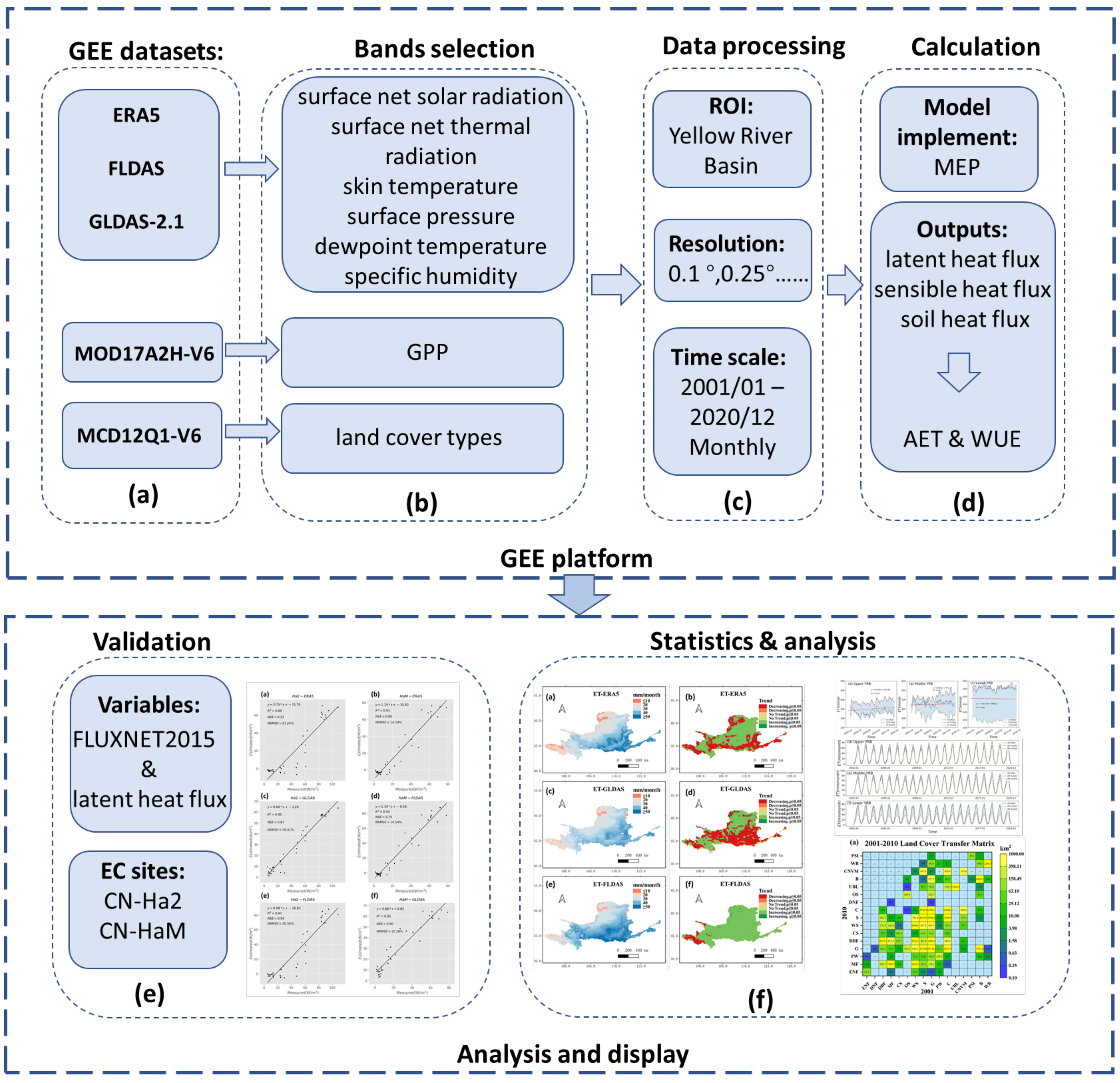
2.1.1. The Proposed Framework
2.1.2. Maximum Entropy Production Method
2.1.3. Statistical Analysis and Post-Processing
Model Performances
Trend Analysis
2.2. Study Area and Data
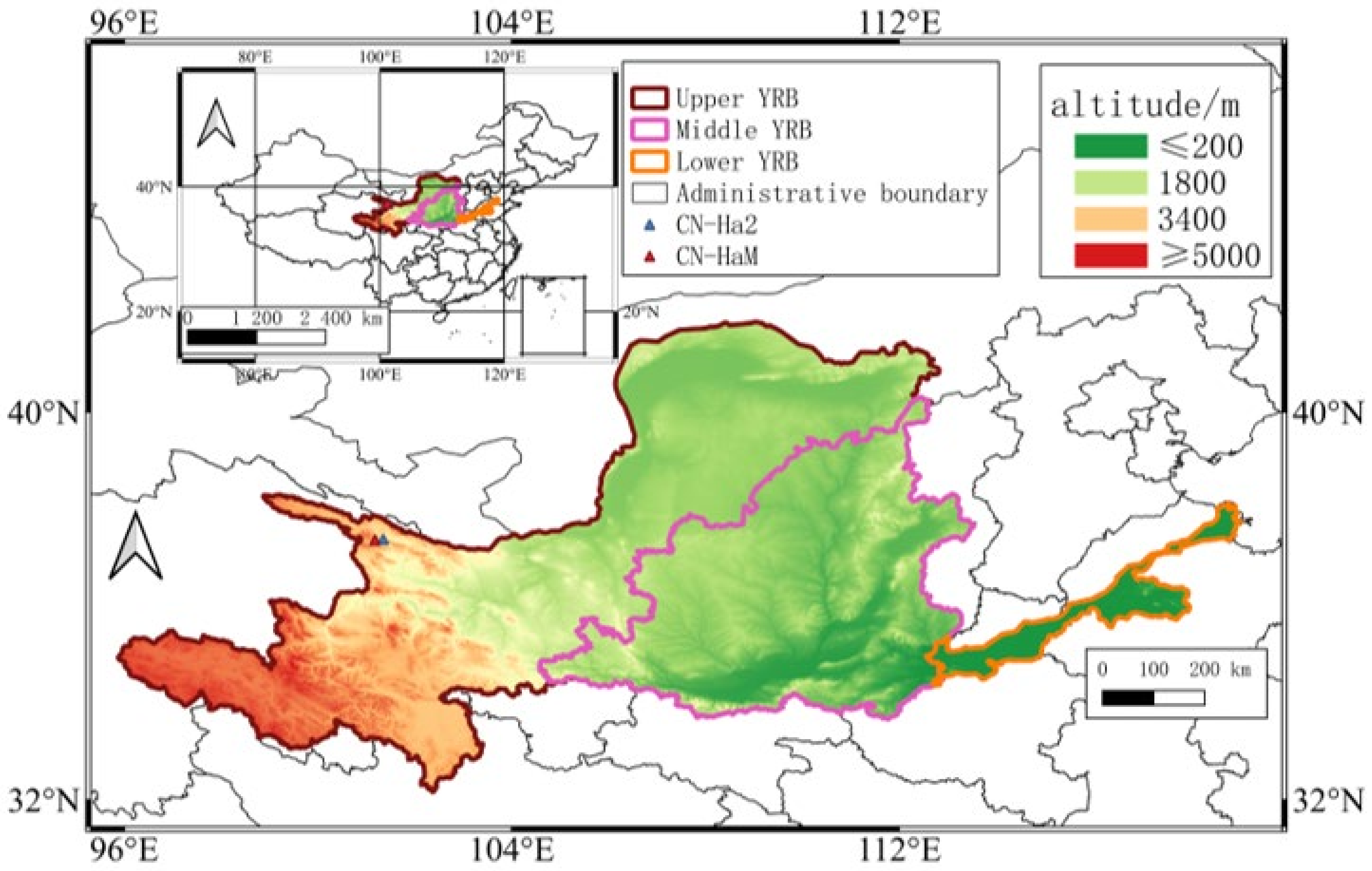
2.2.1. Study Area
2.2.2. Data Sources
Meteorological Variables from Different Datasets
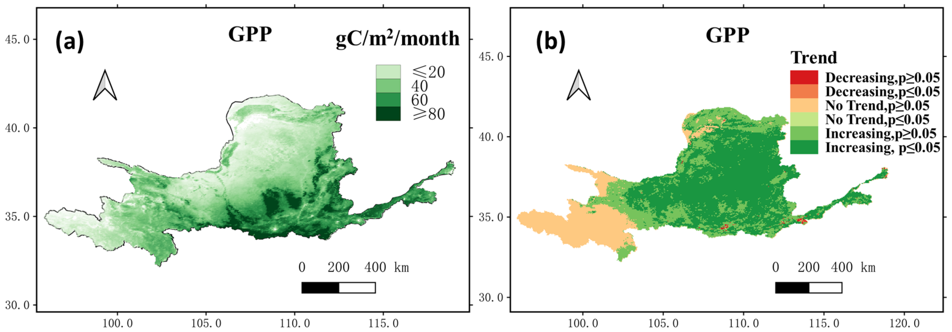
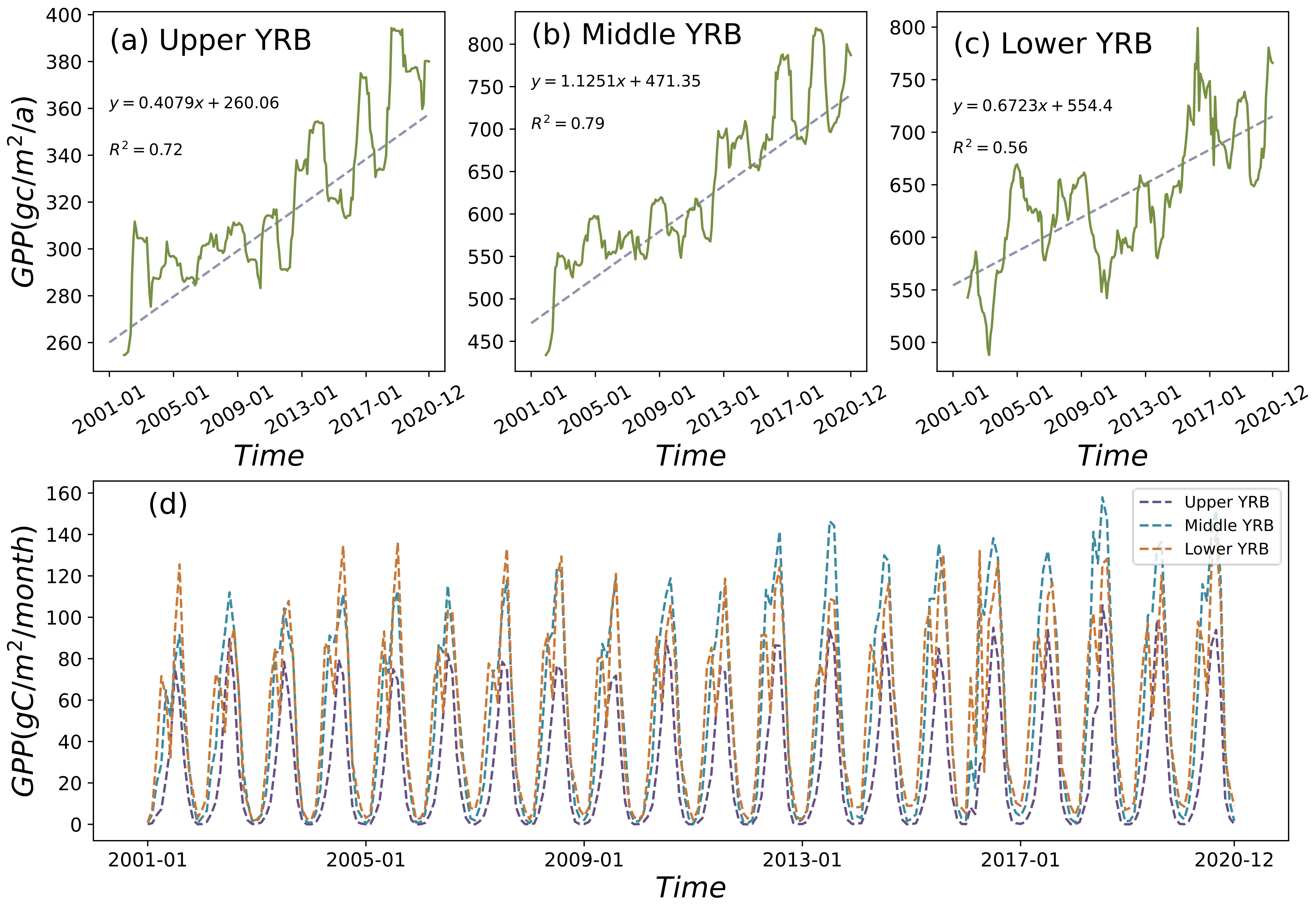
Gross Primary Productivity
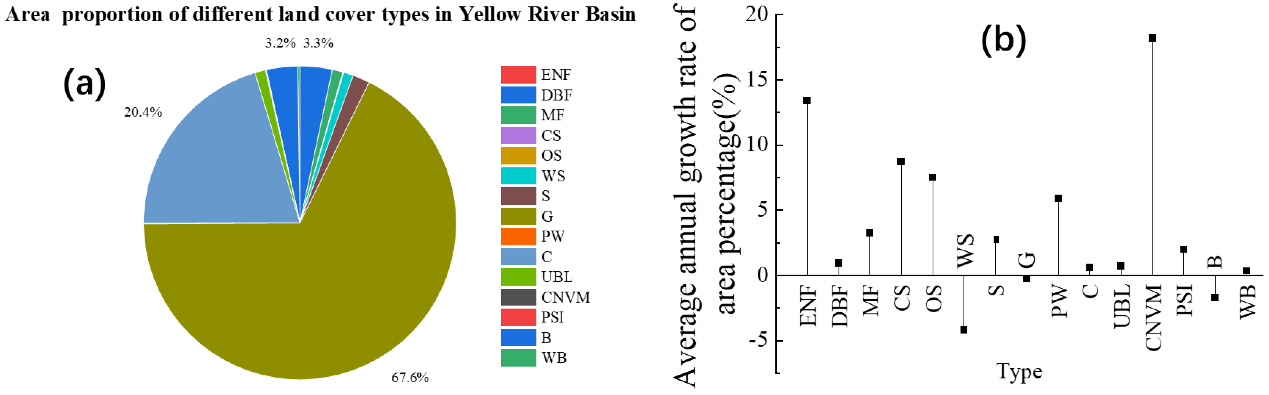
The Landcover Dataset
FLUXNET 2015
3. Results
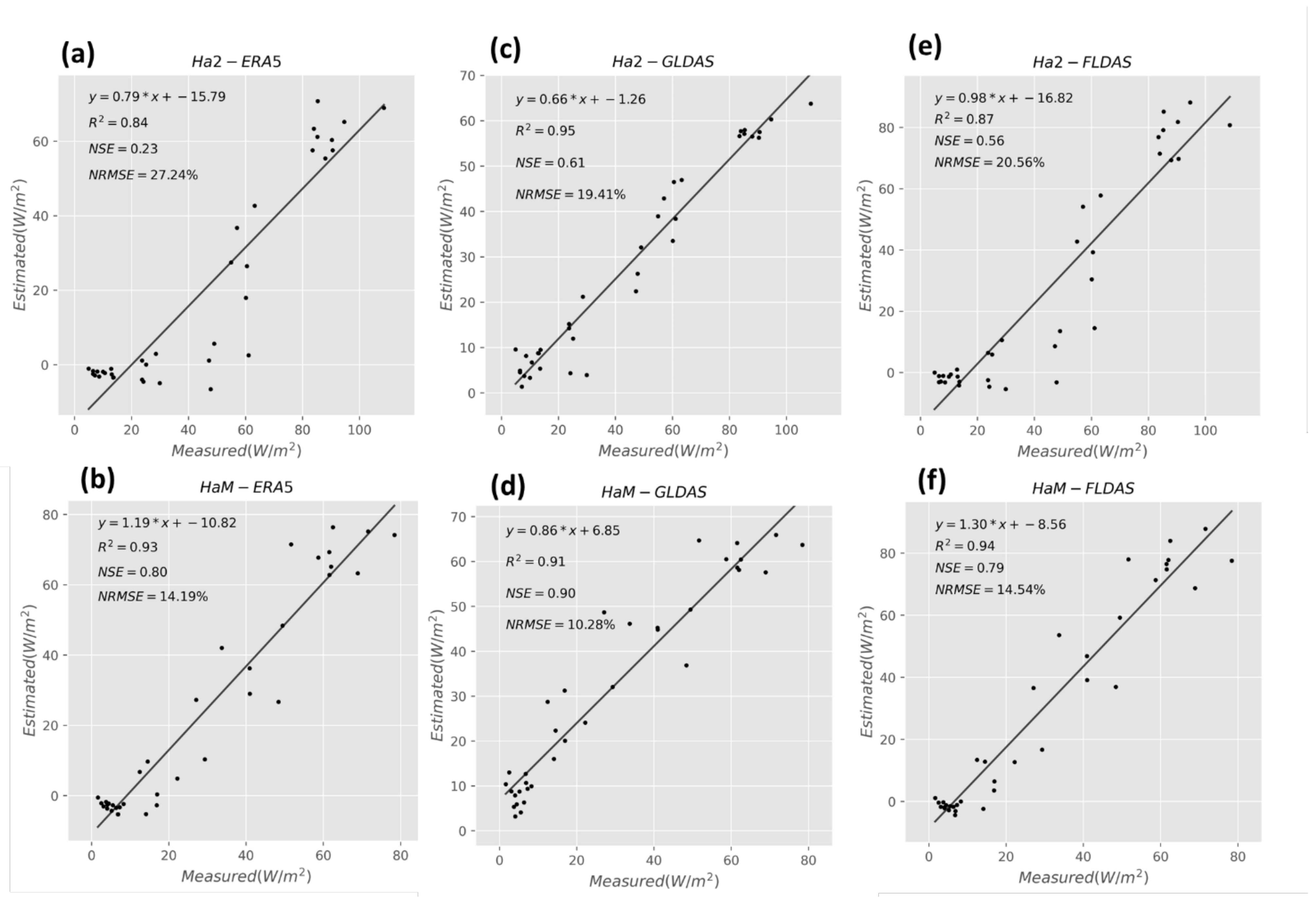
3.1. Validation of Framework for Actual ET
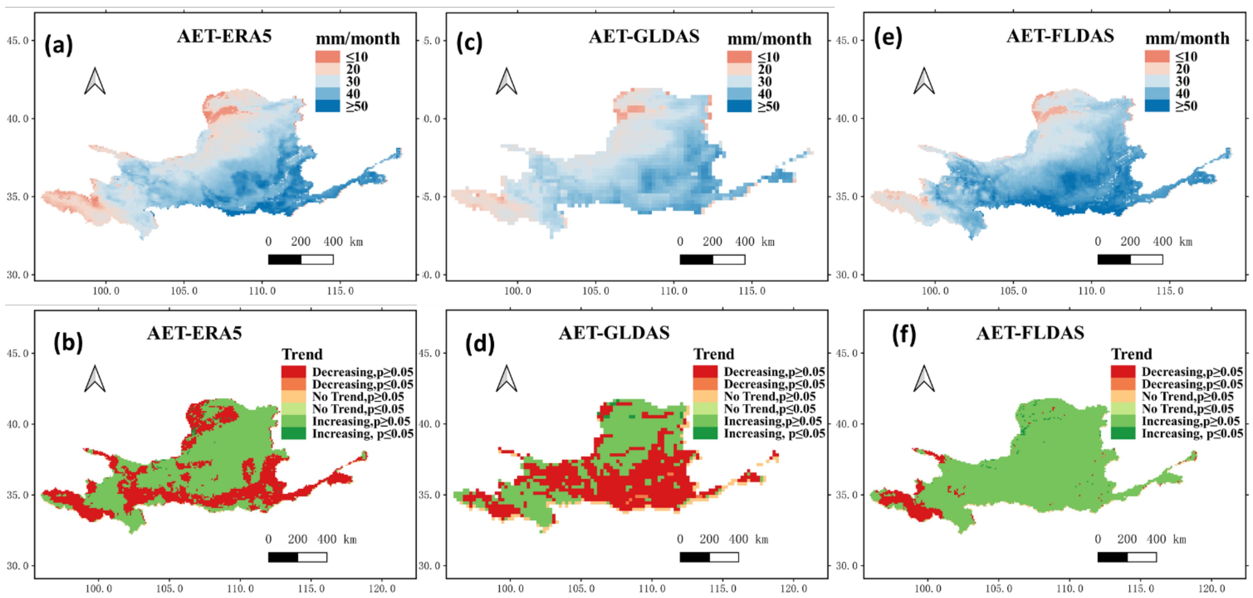
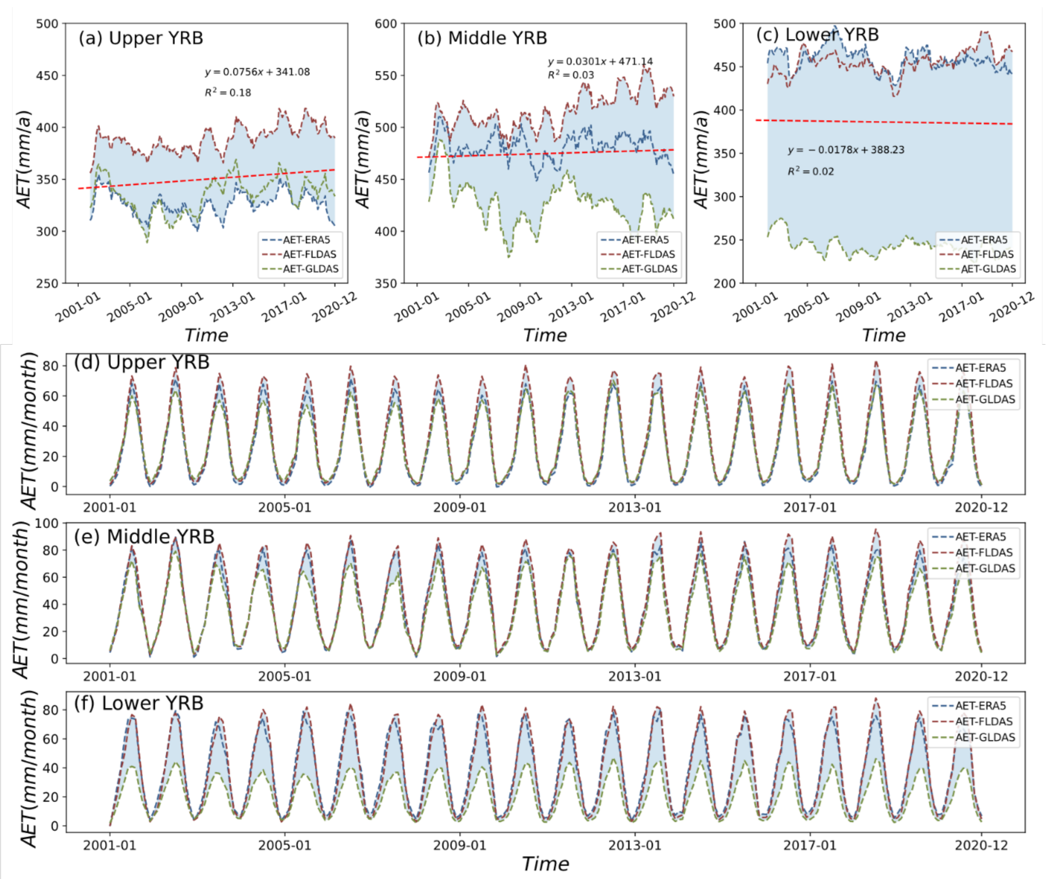
3.2. Spatial–Temporal Variations of Actual ET in the YRB
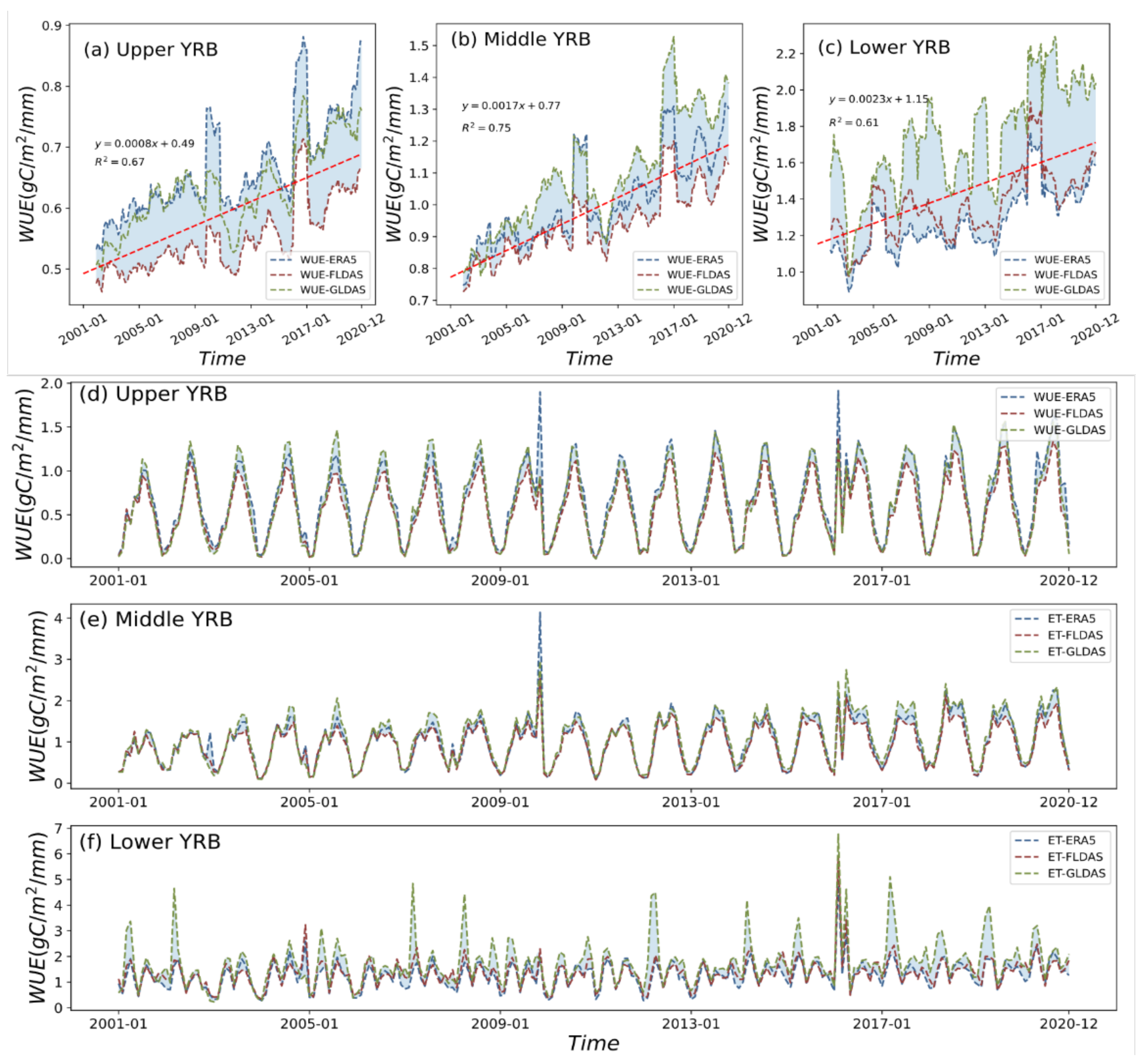
3.3. Spatial–Temporal Variations of WUE in the YRB
3.4. Linkage of WUE Variations and Land-Use Changes
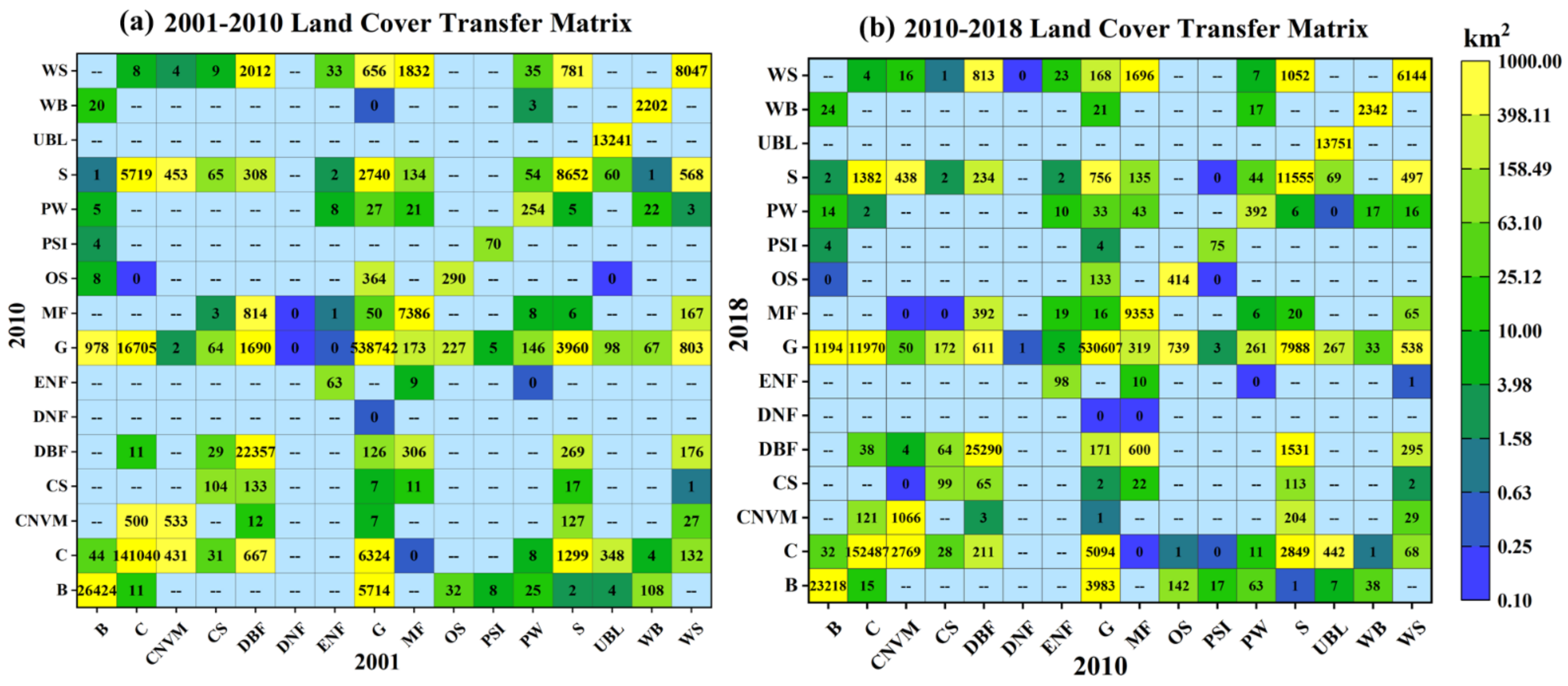
3.4.1. Land-Use Changes in the YRB
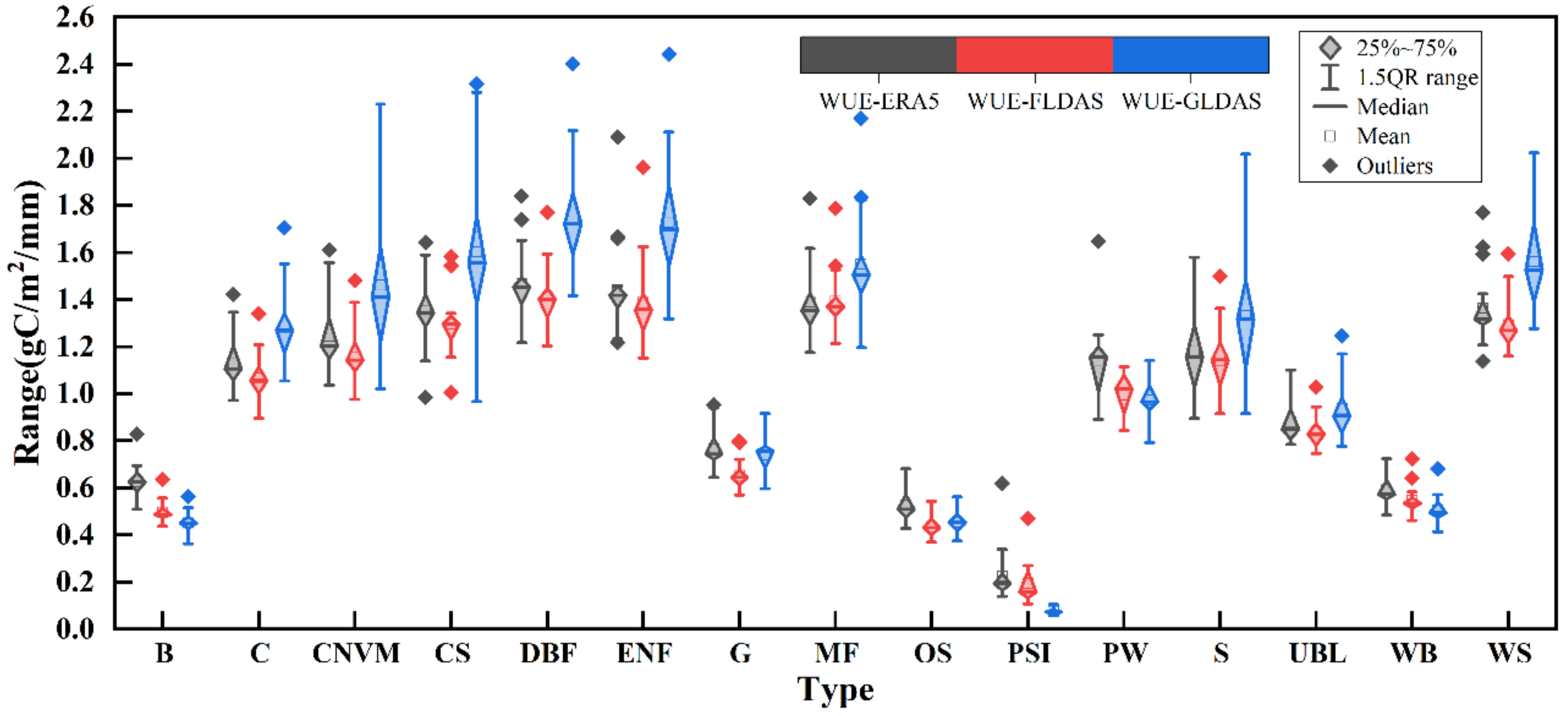
3.4.2. Linkage of WUE Variations and Land-Use Changes
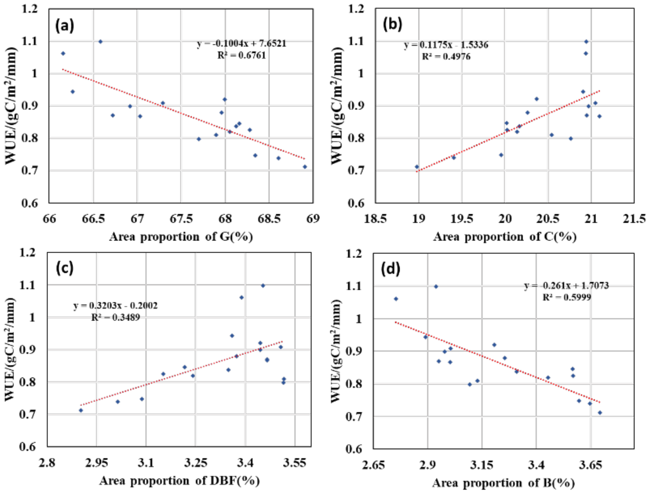
3.4.3. Relationship between WUE Variations and Land-Use Changes
4. Discussion
4.1. Application of the Proposed Framework
4.2. Accuracy Assessment of WUE
4.3. Implications
5. Conclusions
Supplementary Materials
Author Contributions
Funding
Institutional Review Board Statement
Informed Consent Statement
Data Availability Statement
Acknowledgments
Conflicts of Interest
Abbreviations
| WUE | Water use efficiency |
| ET | Evapotranspiration |
| AET | Actual evapotranspiration |
| MEP | Maximum Entropy Production |
| GEE | Google Earth Engine |
| YRB | Yellow River Basin |
| EC | Eddy Covariance |
| SEB | Surface energy balance |
| GEEMEP | Coupling the MEP method and utilizing GEE |
| GDP | Gross Domestic Product |
| GPP | Gross Primary Production |
| ERA5 | ERA5-Land Monthly Averaged—ECMWF Climate Reanalysis |
| FLDAS | Famine Early Warning Systems Network (FEWS NET) Land Data Assimilation System |
| GLDAS-2.1 | Global Land Data Assimilation System |
| MOD17A2H-V6 | Terra Gross Primary Productivity 8-Day Global 500M |
| MCD12Q1-V6 | MODIS Land Cover Type Yearly Global 500m |
| QTP | Qinghai Tibet Plateau |
| IMP | Inner Mongolia Plateau |
| LP | Loess Plateau |
| NCP | North China Plain |
| YRCC | Yellow River Conservancy Commission |
| FEWS NET | The Famine Early Warning Systems Network |
| IGBP | International Geosphere-Biosphere Programmer |
| CN-Ha2 | Haibei Shrubland |
| CN-HaM | Haibei Alpine Tibet Site |
| NSE | Nash–Sutcliffe efficiency |
| NRMSE | Normalized Root Mean Squared Error |
Appendix A


| Value | Description | Abbreviation |
|---|---|---|
| 1 | Evergreen Needleleaf Forests: dominated by evergreen conifer trees (canopy > 2 m). Tree cover > 60%. | ENF |
| 2 | Evergreen Broadleaf Forests: dominated by evergreen broadleaf and palmate trees (canopy > 2 m). Tree cover > 60%. | EBF |
| 3 | Deciduous Needleleaf Forests: dominated by deciduous needleleaf (larch) trees (canopy > 2 m). Tree cover > 60%. | DNF |
| 4 | Deciduous Broadleaf Forests: dominated by deciduous broadleaf trees (canopy > 2 m). Tree cover > 60%. | DBF |
| 5 | Mixed Forests: dominated by neither deciduous nor evergreen (40–60% of each) tree type (canopy > 2 m). Tree cover > 60%. | MF |
| 6 | Closed Shrublands: dominated by woody perennials (1–2 m height) > 60% cover. | CS |
| 7 | Open Shrublands: dominated by woody perennials (1–2 m height) 10–60% cover. | OS |
| 8 | Woody Savannas: tree cover 30–60% (canopy > 2 m). | WS |
| 9 | Savannas: tree cover 10–30% (canopy > 2 m). | S |
| 10 | Grasslands: dominated by herbaceous annuals (<2 m). | G |
| 11 | Permanent Wetlands: permanently inundated lands with 30–60% water cover and > 10% vegetated cover. | PW |
| 12 | Croplands: at least 60% of the area is cultivated cropland. | C |
| 13 | Urban and Built-up Lands: at least 30% impervious surface area including building materials, asphalt and vehicles. | UBL |
| 14 | Cropland/Natural Vegetation Mosaics: mosaics of small-scale cultivation 40–60% with natural tree, shrub, or herbaceous vegetation. | CNVM |
| 15 | Permanent Snow and Ice: at least 60% of the area is covered by snow and ice for at least ten months of the year. | PSI |
| 16 | Barren: at least 60% of the area is non-vegetated barren (sand, rock, soil) areas with less than 10% vegetation. | B |
| 17 | Water Bodies: at least 60% of the area is covered by permanent water bodies. | WB |
References
- Gu, C.; Tang, Q.; Zhu, G.; Ma, J.; Gu, C.; Zhang, K.; Sun, S.; Yu, Q.; Niu, S. Discrepant responses between evapotranspiration-and transpiration-based ecosystem water use efficiency to interannual precipitation fluctuations. Agric. For. Meteorol. 2021, 303, 108385. [Google Scholar] [CrossRef]
- Zhang, L.; Xiao, J.; Zheng, Y.; Li, S.; Zhou, Y. Increased carbon uptake and water use efficiency in global semi-arid ecosystems. Environ. Res. Lett. 2020, 15, 034022. [Google Scholar] [CrossRef]
- Niu, S.; Xing, X.; Zhang, Z.; Xia, J.; Zhou, X.; Song, B.; Li, L.; Wan, S. Water-use efficiency in response to climate change: From leaf to ecosystem in a temperate steppe. Glob. Change Biol. 2011, 17, 1073–1082. [Google Scholar] [CrossRef]
- Beer, C.; Ciais, P.; Reichstein, M.; Baldocchi, D.; Law, B.E.; Papale, D.; Soussana, J.F.; Ammann, C.; Buchmann, N.; Frank, D.; et al. Temporal and among-site variability of inherent water use efficiency at the ecosystem level. Glob. Biogeochem. Cycles 2009, 23, e2008GB003233. [Google Scholar] [CrossRef]
- Chapin, F.S.; Matson, P.A.; Vitousek, P. Principles of Terrestrial Ecosystem Ecology; Springer: New York, NY, USA, 2011. [Google Scholar]
- DeLucia, E.H.; Heckathorn, S.A. The effect of soil drought on water-use efficiency in a contrasting Great Basin desert and Sierran montane species. Plant Cell Environ. 1989, 12, 935–940. [Google Scholar] [CrossRef]
- Lasch, P.; Lindner, M.; Erhard, M.; Suckow, F.; Wenzel, A. Regional impact assessment on forest structure and functions under climate change—The Brandenburg case study. For. Ecol. Manag. 2002, 162, 73–86. [Google Scholar] [CrossRef]
- Zhu, Q.; Jiang, H.; Peng, C.; Liu, J.; Wei, X.; Fang, X.; Liu, S.; Zhou, G.; Yu, S. Evaluating the effects of future climate change and elevated CO2 on the water use efficiency in terrestrial ecosystems of China. Ecol. Model. 2011, 222, 2414–2429. [Google Scholar] [CrossRef]
- Jing, Z.; Cheng, L.; Zhang, L.; Wang, Y.-P.; Liu, P.; Zhang, X.; Wang, Q. The dependence of ecosystem water use partitioning on vegetation productivity at the inter-annual time scale. J. Geophys. Res. Atmos. 2021, 126, e2020JD033756. [Google Scholar] [CrossRef]
- Katul, G.G.; Oren, R.; Manzoni, S.; Higgins, C.; Parlange, M.B. Evapotranspiration: A process driving mass transport and energy exchange in the soil-plant-atmosphere-climate system. Rev. Geophys. 2012, 50, e2011rg000366. [Google Scholar] [CrossRef] [Green Version]
- Duan, Z.; Bastiaanssen, W. Evaluation of three energy balance-based evaporation models for estimating monthly evaporation for five lakes using derived heat storage changes from a hysteresis model. Environ. Res. Lett. 2017, 12, 024005. [Google Scholar] [CrossRef] [Green Version]
- Cao, M.; Wang, W.; Xing, W.; Wei, J.; Chen, X.; Li, J.; Shao, Q. Multiple sources of uncertainties in satellite retrieval of terrestrial actual evapotranspiration. J. Hydrol. 2021, 601, 126642. [Google Scholar] [CrossRef]
- Cook, D.R. Energy Balance Bowen Ratio (EBBR) Handbook. 2005. Available online: https://www.osti.gov/biblio/1020562-energy-balance-bowen-ratio-station-ebbr-instrument-handbook (accessed on 9 December 2021).
- Goss, M.J.; Ehlers, W. The role of lysimeters in the development of our understanding of soil water and nutrient dynamics in ecosystems. Soil Use Manag. 2009, 25, 213–223. [Google Scholar] [CrossRef]
- Su, Z. The Surface Energy Balance System (SEBS) for estimation of turbulent heat fluxes. Hydrol. Earth Syst. Sci. 2002, 6, 85–100. [Google Scholar] [CrossRef]
- Wang, W.; Li, J.; Yu, Z.; Ding, Y.; Xing, W.; Lu, W. Satellite retrieval of actual evapotranspiration in the Tibetan Plateau: Components partitioning, multidecadal trends and dominated factors identifying. J. Hydrol. 2018, 559, 471–485. [Google Scholar] [CrossRef]
- Wang, K.; Dickinson, R.E. A review of global terrestrial evapotranspiration: Observation, modeling, climatology, and climatic variability. Rev. Geophys. 2012, 50, e2011rg000373. [Google Scholar] [CrossRef]
- Wilson, K.; Goldstein, A.; Falge, E.; Aubinet, M.; Baldocchi, D.; Berbigier, P.; Bernhofer, C.; Ceulemans, R.; Dolman, H.; Field, C.; et al. Energy balance closure at FLUXNET sites. Agric. For. Meteorol. 2002, 113, 223–243. [Google Scholar] [CrossRef] [Green Version]
- Elnashar, A.; Wang, L.; Wu, B.; Zhu, W.; Zeng, H. Synthesis of global actual evapotranspiration from 1982 to 2019. Earth Syst. Sci. Data 2021, 13, 447–480. [Google Scholar] [CrossRef]
- Oki, T.; Kanae, S. Global hydrological cycles and world water resources. Science 2006, 313, 1068–1072. [Google Scholar] [CrossRef] [Green Version]
- Rodell, M.; Beaudoing, H.K.; L’Ecuyer, T.S.; Olson, W.S.; Famiglietti, J.S.; Houser, P.R.; Adler, R.; Bosilovich, M.G.; Clayson, C.A.; Chambers, D.; et al. The observed state of the water cycle in the early twenty-first century. J. Clim. 2015, 28, 8289–8318. [Google Scholar] [CrossRef]
- Trenberth, K.E.; Smith, L.; Qian, T.; Dai, A.; Fasullo, J. Estimates of the global water budget and its annual cycle using observational and model data. J. Hydrometeorol. 2007, 8, 758–769. [Google Scholar] [CrossRef]
- Jepsen, S.; Harmon, T.C.; Guan, B. Analyzing the Suitability of Remotely Sensed ET for Calibrating a Watershed Model of a Mediterranean Montane Forest. Remote Sens. 2021, 13, 1258. [Google Scholar] [CrossRef]
- Zhang, K.; Zhu, G.; Ma, J.; Yang, Y.; Shang, S.; Gu, C. Parameter analysis and estimates for the MODIS evapotranspiration algorithm and multiscale verification. Water Resour. Res. 2019, 55, 2211–2231. [Google Scholar] [CrossRef]
- Sun, H.; Yang, Y.; Wu, R.; Gui, D.; Xue, J.; Liu, Y.; Yan, D. Improving estimation of cropland evapotranspiration by the Bayesian model averaging method with surface energy balance models. Atmosphere 2019, 10, 188. [Google Scholar] [CrossRef] [Green Version]
- Yang, Z.; Tian, J.; Li, W.; Su, W.; Guo, R.; Liu, W. Spatio-temporal pattern and evolution trend of ecological environment quality in the Yellow River Basin. Acta Ecol. Sin. 2021, 41, 7627–7636. [Google Scholar]
- Wang, J.; Bras, R.L. A model of evapotranspiration based on the theory of maximum entropy production. Water Resour. Res. 2011, 47, e2010wr009392. [Google Scholar] [CrossRef]
- Hajji, I.; Nadeau, D.F.; Music, B.; Anctil, F.; Wang, J. Application of the maximum entropy production model of evapotranspiration over partially vegetated water-limited land surfaces. J. Hydrometeorol. 2018, 19, 989–1005. [Google Scholar] [CrossRef]
- El Sharif, H.; Zhou, W.; Ivanov, V.; Sheshukov, A.; Mazepa, V.; Wang, J. Surface energy budgets of Arctic tundra during growing season. J. Geophys. Res. Atmos. 2019, 124, 6999–7017. [Google Scholar] [CrossRef]
- Xu, D.; Agee, E.; Wang, J.; Ivanov, V.Y. Estimation of evapotranspiration of Amazon rainforest using the maximum entropy production method. Geophys. Res. Lett. 2019, 46, 1402–1412. [Google Scholar] [CrossRef]
- Timmermans, W.J.; Kustas, W.P.; Anderson, M.C.; French, A.N. An intercomparison of the surface energy balance algorithm for land (SEBAL) and the two-source energy balance (TSEB) modeling schemes. Remote Sens. Environ. 2007, 108, 369–384. [Google Scholar] [CrossRef]
- Bastiaanssen, W.G.M.; Menenti, M.; Feddes, R.A.; Holtslag, A.A.M. A remote sensing surface energy balance algorithm for land (SEBAL). 1. Formulation. J. Hydrol. 1998, 212–213, 198–212. [Google Scholar] [CrossRef]
- Khan, M.S.; Liaqat, U.W.; Baik, J.; Choi, M. Stand-alone uncertainty characterization of GLEAM, GLDAS and MOD16 evapotranspiration products using an extended triple collocation approach. Agric. For. Meteorol. 2018, 252, 256–268. [Google Scholar] [CrossRef]
- Vinukollu, R.K.; Wood, E.F.; Ferguson, C.R.; Fisher, J.B. Global estimates of evapotranspiration for climate studies using multi-sensor remote sensing data: Evaluation of three process-based approaches. Remote Sens. Environ. 2011, 115, 801–823. [Google Scholar] [CrossRef]
- Yao, Y.; Liang, S.; Cheng, J.; Liu, S.; Fisher, J.B.; Zhang, X.; Jia, K.; Zhao, X.; Qin, Q.; Zhao, B.; et al. MODIS-driven estimation of terrestrial latent heat flux in China based on a modified Priestley–Taylor algorithm. Agric. For. Meteorol. 2013, 171–172, 187–202. [Google Scholar] [CrossRef]
- Kumar, L.; Mutanga, O. Google Earth Engine applications since inception: Usage, trends, and potential. Remote Sens. 2018, 10, 1509. [Google Scholar] [CrossRef] [Green Version]
- Gorelick, N.; Hancher, M.; Dixon, M.; Ilyushchenko, S.; Thau, D.; Moore, R. Google Earth Engine: Planetary-scale geospatial analysis for everyone. Remote Sens. Environ. 2017, 202, 18–27. [Google Scholar] [CrossRef]
- Li, C.C.; Zhang, Y.Q.; Shen, Y.J.; Yu, Q. Decadal water storage decrease driven by vegetation changes in the Yellow River Basin. Sci. Bull. 2020, 65, 1859–1861. [Google Scholar] [CrossRef]
- Tang, Q.; Oki, T.; Kanae, S.; Hu, H. A spatial analysis of hydro-climatic and vegetation condition trends in the Yellow River basin. Hydrol. Process. 2008, 22, 451–458. [Google Scholar] [CrossRef]
- Tang, Q.; Vivoni, E.R.; Muñoz-Arriola, F.; Lettenmaier, D.P. Predictability of evapotranspiration patterns using remotely sensed vegetation dynamics during the North American monsoon. J. Hydrometeorol. 2012, 13, 103–121. [Google Scholar] [CrossRef]
- Sun, H.; Bai, Y.; Lu, M.; Wang, J.; Tuo, Y.; Yan, D.; Zhang, W. Drivers of the water use efficiency changes in China during 1982–2015. Sci. Total Environ. 2021, 799, 149145. [Google Scholar] [CrossRef]
- Hu, Z.M.; Yu, G.R.; Wang, Q.F.; Zhao, F.H. Ecosystem level water use efficiency: A review. Acta Ecol. Sin. 2009, 29, 1498–1507. [Google Scholar]
- Tang, Y.; Shahnaz, S.; Wang, J. A Non-gradient Model of Turbulent Gas Fluxes over Land Surfaces. J. Geophys. Res. Atmos. 2021, 126, e2021JD034605. [Google Scholar] [CrossRef]
- Wang, J.; Bras, R.L. An extremum solution of the Monin–Obukhov similarity equations. J. Atmos. Sci. 2010, 67, 485–499. [Google Scholar] [CrossRef]
- Amani, M.; Ghorbanian, A.; Ahmadi, S.A.; Kakooei, M.; Moghimi, A.; Mirmazloumi, S.M.; Moghaddam, S.H.A.; Mahdavi, S.; Ghahremanloo, M.; Parsian, S.; et al. Google earth engine cloud computing platform for remote sensing big data applications: A comprehensive review. IEEE J. Sel. Top. Appl. Earth Obs. Remote Sens. 2020, 13, 5326–5350. [Google Scholar] [CrossRef]
- Wang, J.; Bras, R.L. A model of surface heat fluxes based on the theory of maximum entropy production. Water Resour. Res. 2009, 45, e2009WR007900. [Google Scholar] [CrossRef] [Green Version]
- Chen, Y.; Yang, K.; He, J.; Qin, J.; Shi, J.; Du, J.; He, Q. Improving land surface temperature modeling for dry land of China. J. Geophys. Res. Atmos. 2011, 116, e2011jd015921. [Google Scholar] [CrossRef]
- Bolton, D. The computation of equivalent potential temperature. Mon. Weather Rev. 1980, 108, 1046–1053. [Google Scholar] [CrossRef] [Green Version]
- Gupta, H.V.; Kling, H.; Yilmaz, K.K.; Martinez, G.F. Decomposition of the mean squared error and NSE performance criteria: Implications for improving hydrological modelling. J. Hydrol. 2009, 377, 80–91. [Google Scholar] [CrossRef] [Green Version]
- Yang, Y.; Sun, H.; Luo, H. Application of maximum entropy production model for estimation of evapotranspiration in China. Agric. Res. Arid. Areas 2020, 38, 184–191. [Google Scholar]
- Helsel, D.R.; Hirsch, R.M. Statistical Methods in Water Resources. Techniques of Water-Resources Investigations of the United States Geological Survey; United States Geological Survey: Reston, VA, USA, 2002; p. 522.
- Mann, H.B. Nonparametric tests against trend. Econometrica 1945, 13, 245–259. [Google Scholar] [CrossRef]
- Azizzadeh, M.; Javan, K. Analyzing trends in reference evapotranspiration in northwest part of Iran. J. Ecol. Eng. 2015, 16, 1–12. [Google Scholar] [CrossRef]
- Shadmani, M.; Marofi, S.; Roknian, M. Trend analysis in reference evapotranspiration using Mann-Kendall and Spearman’s Rho tests in arid regions of Iran. Water Resour. Manag. 2012, 26, 211–224. [Google Scholar] [CrossRef] [Green Version]
- Omer, A.; Zhuguo, M.; Zheng, Z.; Saleem, F. Natural and anthropogenic influences on the recent droughts in Yellow River Basin, China. Sci. Total Environ. 2020, 704, 135428. [Google Scholar] [CrossRef]
- Muñoz Sabater, J. ERA5-Land Monthly Averaged Data from 1981 to Present; Copernicus Climate Change Service (C3S), Climate Data Store (CDS) [Data Set]. 2019. Available online: https://cds.climate.copernicus.eu/cdsapp#!/dataset/10.24381/cds.68d2bb30?tab=overview (accessed on 9 December 2021).
- Rodell, M.; Houser, P.R.; Jambor, U.; Gottschalck, J.; Mitchell, K.; Meng, C.; Arsenault, K.; Cosgrove, B.; Radakovich, J.; Bosilovich, M. The global land data assimilation system. Bull. Am. Meteorol. Soc. 2004, 85, 381–394. [Google Scholar] [CrossRef] [Green Version]
- McNally, A. FLDAS noah land surface model L4 global monthly 0.1 × 0.1 degree (MERRA-2 and CHIRPS). Atmos. Compos. Water Energy Cycles Clim. Var. 2018. [Google Scholar] [CrossRef]
- Sulla-Menashe, D.; Friedl, M. MCD12Q1 MODIS/Terra+Aqua Land Cover Type Yearly L3 Llobal 500 m SIN Grid v006; NASA EOSDIS Land Processes DAAC: Sioux Falls, SD, USA, 2019. [Google Scholar]
- Pastorello, G.; Trotta, C.; Canfora, E.; Chu, H.; Christianson, D.; Cheah, Y.-W.; Poindexter, C.; Chen, J.; Elbashandy, A.; Humphrey, M.; et al. The FLUXNET2015 dataset and the ONEFlux processing pipeline for eddy covariance data. Sci. Data 2020, 7, 225. [Google Scholar] [CrossRef] [PubMed]
- Reba, M.L.; Link, T.E.; Marks, D.; Pomeroy, J. An assessment of corrections for eddy covariance measured turbulent fluxes over snow in mountain environments. Water Resour. Res. 2009, 45, e2008WR007045. [Google Scholar] [CrossRef]
- Junttila, S.; Kelly, J.; Kljun, N.; Aurela, M.; Klemedtsson, L.; Lohila, A.; Nilsson, M.B.; Rinne, J.; Tuittila, E.; Vestin, P.; et al. Upscaling northern peatland CO2 fluxes using satellite remote sensing data. Remote Sens. 2021, 13, 818. [Google Scholar] [CrossRef]

| Dataset | Spatial Resolution | Time Resolution | Index in GEE | Bands Selected in Datasets | Units |
|---|---|---|---|---|---|
| GPP | 500m | 8-day | MODIS/006/MOD17A2H | Gpp | kg·C/m2 |
| Land cover | 500m | yearly | MODIS/006/MCD12Q1 | LC_Type1 | |
| ERA5 | 0.1° | monthly | ECMWF/ERA5_LAND/MONTHLY | surface_net_solar_radiation surface_net_thermal_radiation skin_temperature surface_pressure dewpoint_temperature_2m | J/m2 J/m2 K K K |
| FLDAS | 0.1° | monthly | NASA/FLDAS/NOAH01/C/GL/M/V001 | Qair_f_tavg Swnet_tavg Lwnet_tavg RadT_tavg Psurf_f_tavg | kg/kg W/m2 W/m2 K Pa |
| GLDAS | 0.25° | 3-hourly | NASA/GLDAS/V021/NOAH/G025/T3H | Qair_f_inst Swnet_tavg Lwnet_tavg AvgSurfT_inst | kg/kg W/m2 W/m2 K |
| Sub-Basin | AET | GPP | WUE | |||
|---|---|---|---|---|---|---|
| Multi-Years Mean (mm/a) | Slope (mm/a2) | Multi-Years Mean (gC/m2.a) | Slope (gC/m2.a2) | Multi-Years Mean (gC/m2/mm) | Slope (gC/m2.mm1.a) | |
| Upper | 350.13 | 0.08 | 321.03 | 0.41 | 0.62 | 0.0008 |
| Middle | 474.52 | 0.03 | 635.06 | 1.13 | 1.02 | 0.0017 |
| Lower | 385.73 | −0.02 | 637.34 | 0.67 | 1.46 | 0.0023 |
Publisher’s Note: MDPI stays neutral with regard to jurisdictional claims in published maps and institutional affiliations. |
© 2022 by the authors. Licensee MDPI, Basel, Switzerland. This article is an open access article distributed under the terms and conditions of the Creative Commons Attribution (CC BY) license (https://creativecommons.org/licenses/by/4.0/).
Share and Cite
Sun, H.; Chen, L.; Yang, Y.; Lu, M.; Qin, H.; Zhao, B.; Lu, M.; Xue, J.; Yan, D. Assessing Variations in Water Use Efficiency and Linkages with Land-Use Changes Using Three Different Data Sources: A Case Study of the Yellow River, China. Remote Sens. 2022, 14, 1065. https://doi.org/10.3390/rs14051065
Sun H, Chen L, Yang Y, Lu M, Qin H, Zhao B, Lu M, Xue J, Yan D. Assessing Variations in Water Use Efficiency and Linkages with Land-Use Changes Using Three Different Data Sources: A Case Study of the Yellow River, China. Remote Sensing. 2022; 14(5):1065. https://doi.org/10.3390/rs14051065
Chicago/Turabian StyleSun, Huaiwei, Lin Chen, Yong Yang, Mengge Lu, Hui Qin, Bingqian Zhao, Mengtian Lu, Jie Xue, and Dong Yan. 2022. "Assessing Variations in Water Use Efficiency and Linkages with Land-Use Changes Using Three Different Data Sources: A Case Study of the Yellow River, China" Remote Sensing 14, no. 5: 1065. https://doi.org/10.3390/rs14051065
APA StyleSun, H., Chen, L., Yang, Y., Lu, M., Qin, H., Zhao, B., Lu, M., Xue, J., & Yan, D. (2022). Assessing Variations in Water Use Efficiency and Linkages with Land-Use Changes Using Three Different Data Sources: A Case Study of the Yellow River, China. Remote Sensing, 14(5), 1065. https://doi.org/10.3390/rs14051065