
A Maritime Cloud-Detection Method Using Visible and Near-Infrared Bands over the Yellow Sea and Bohai Sea


Abstract
:1. Introduction
2. Methods
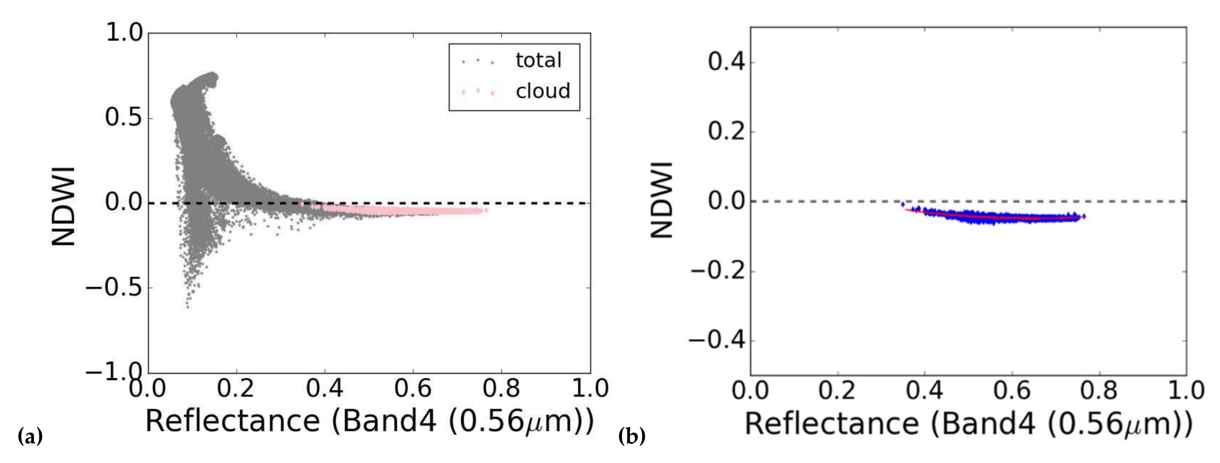
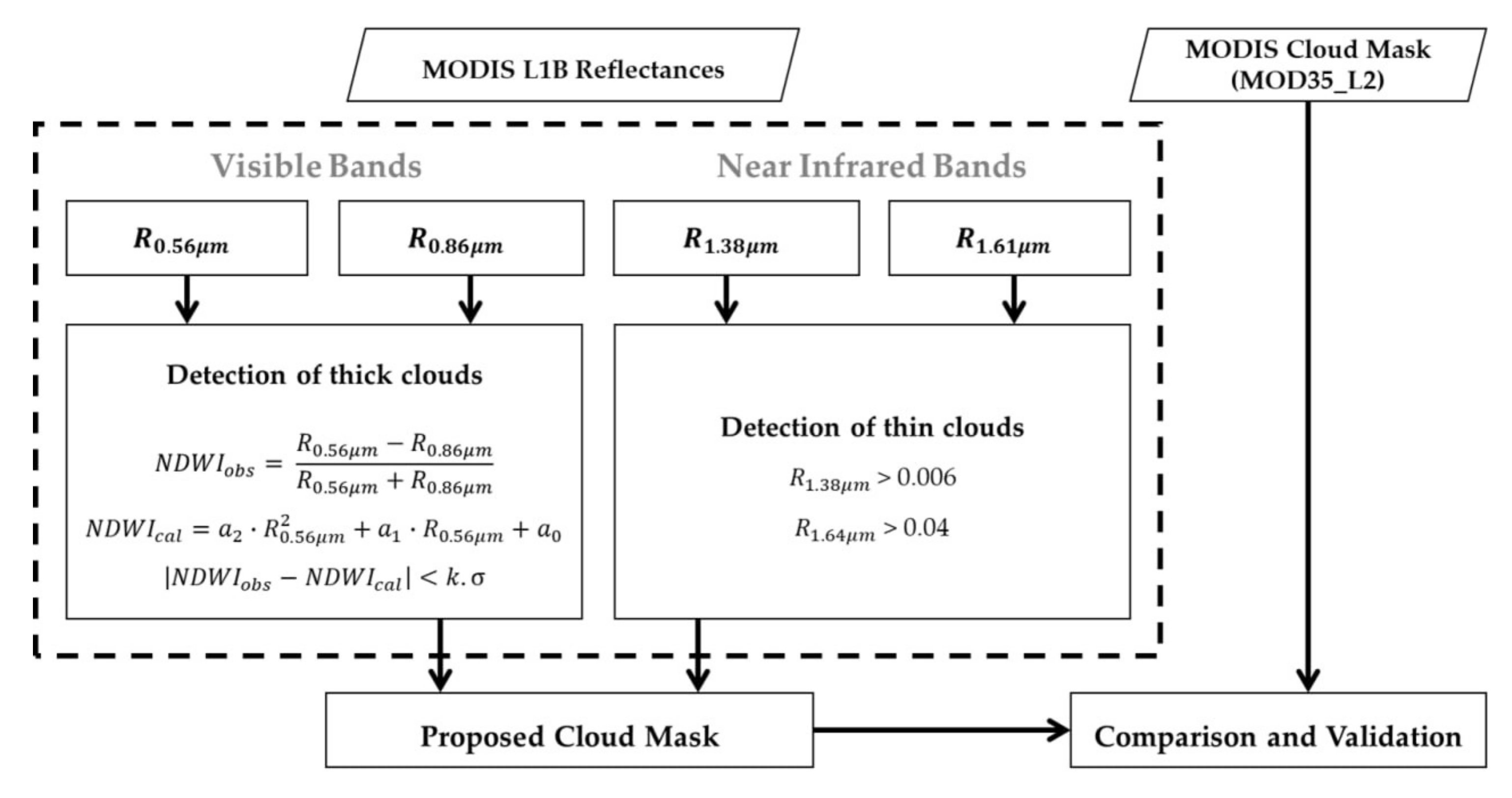
2.1. Cloud Detection Method
2.2. Comparison
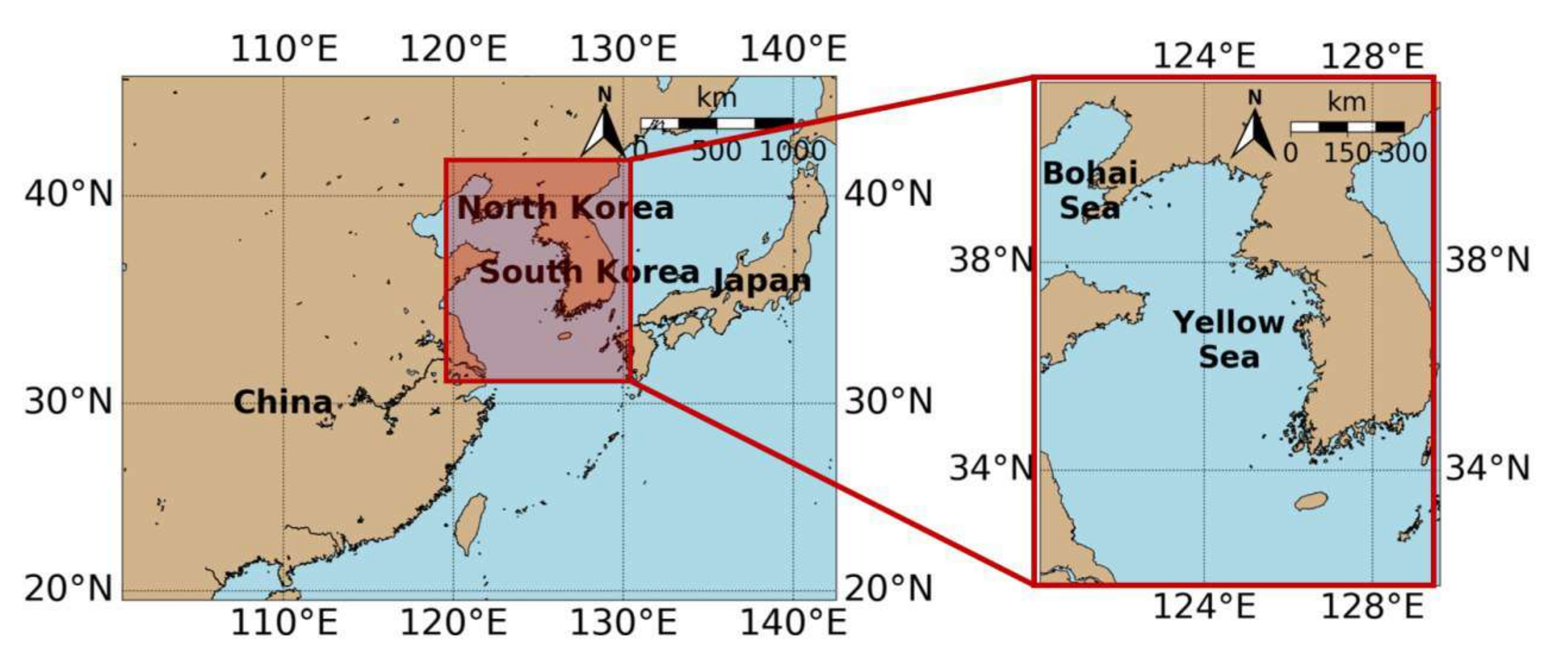
3. Study Area and Data
3.1. MODIS
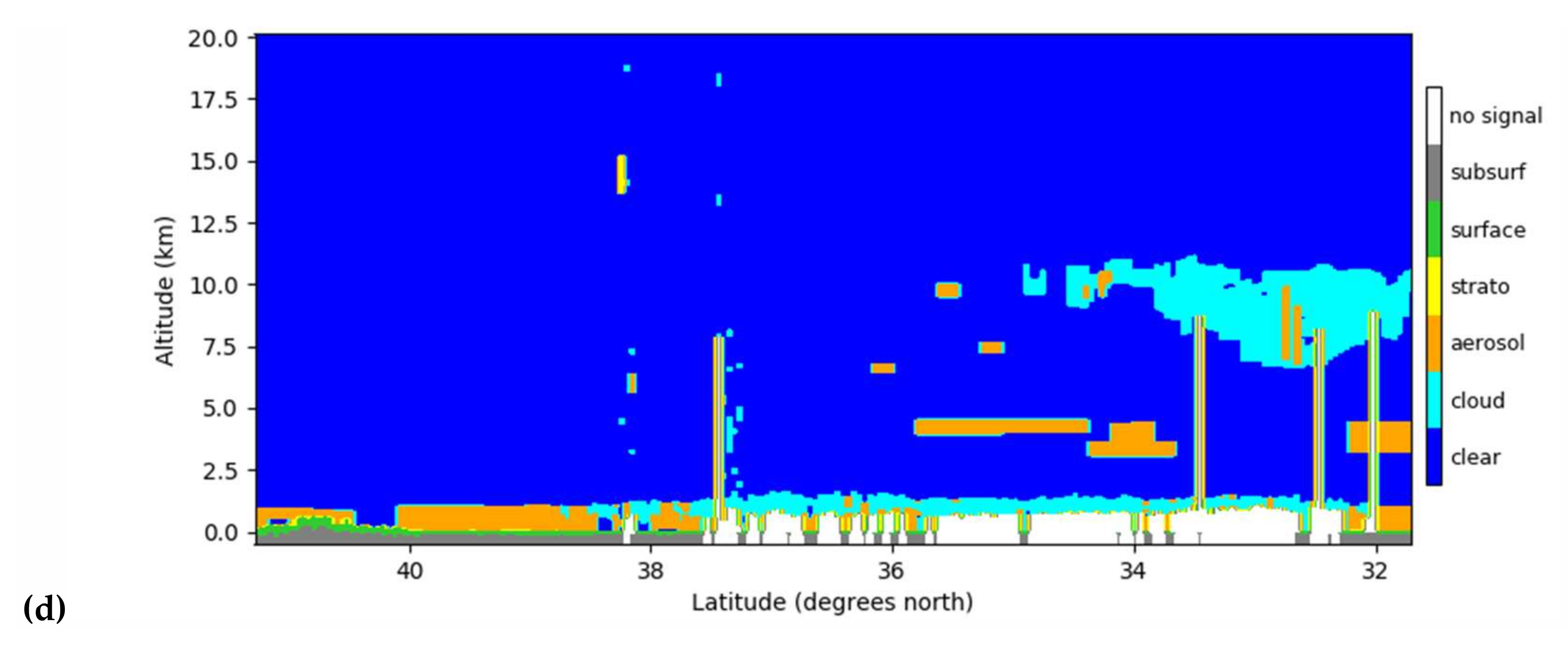
3.2. CALIPSO
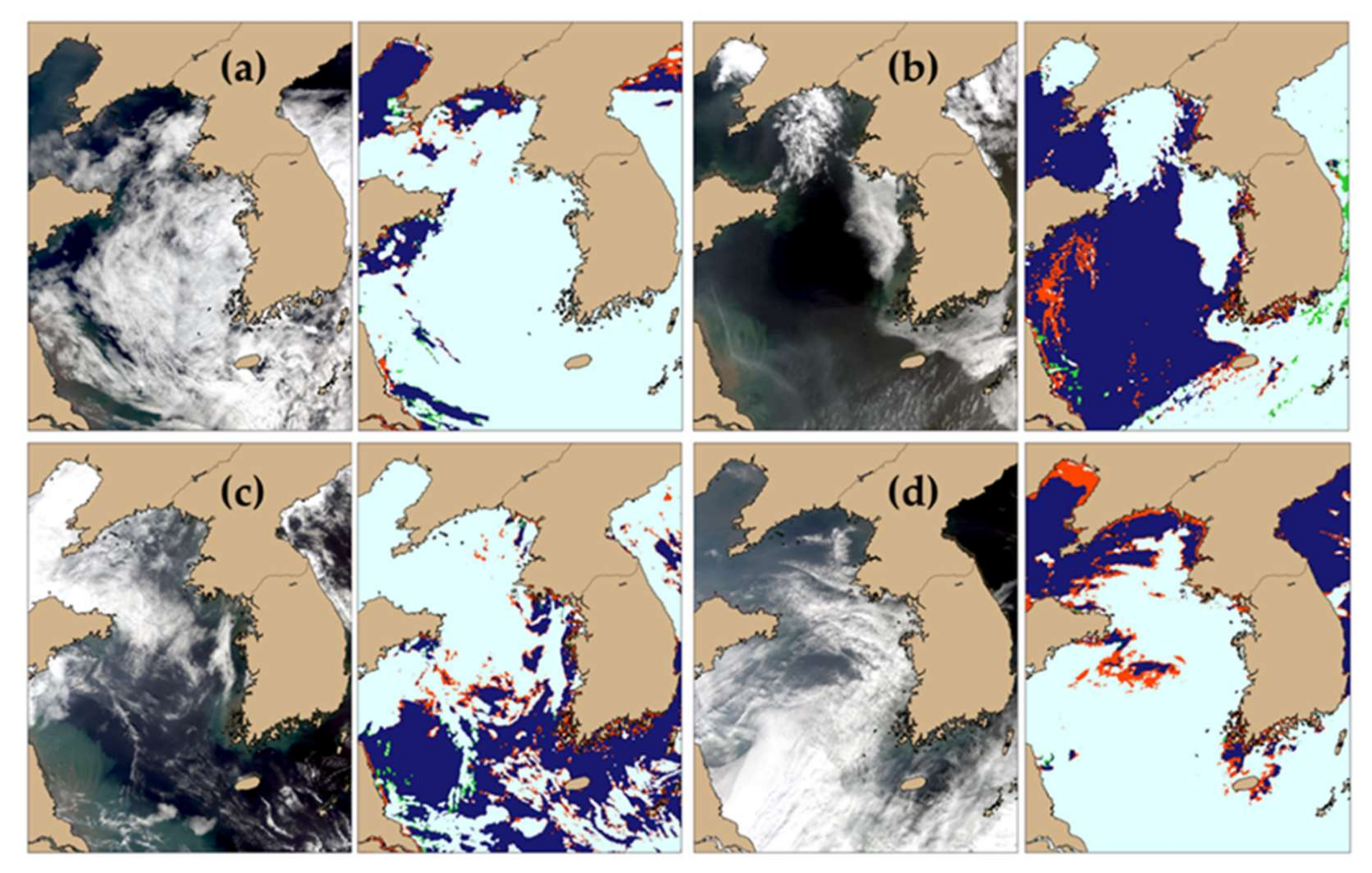
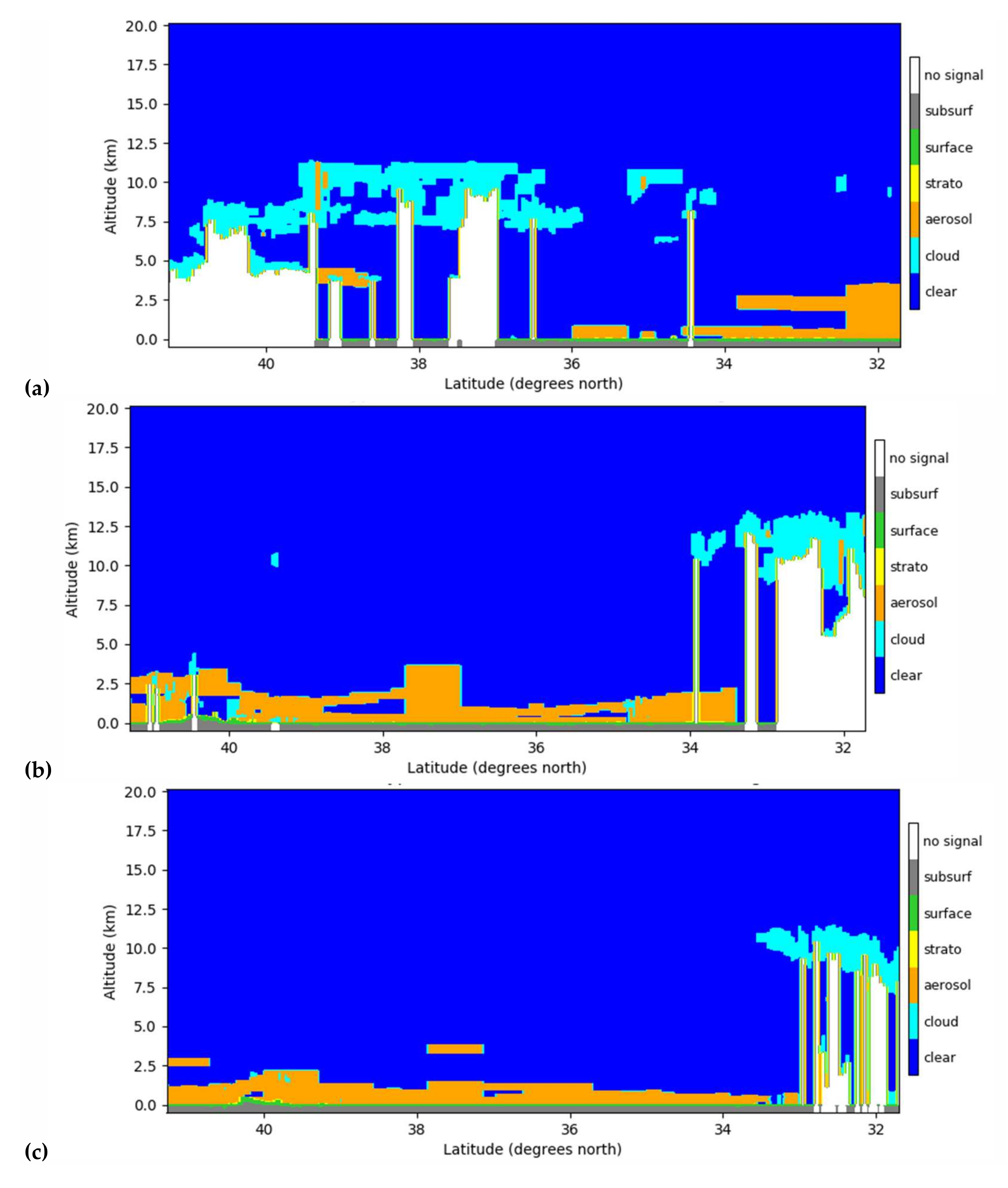
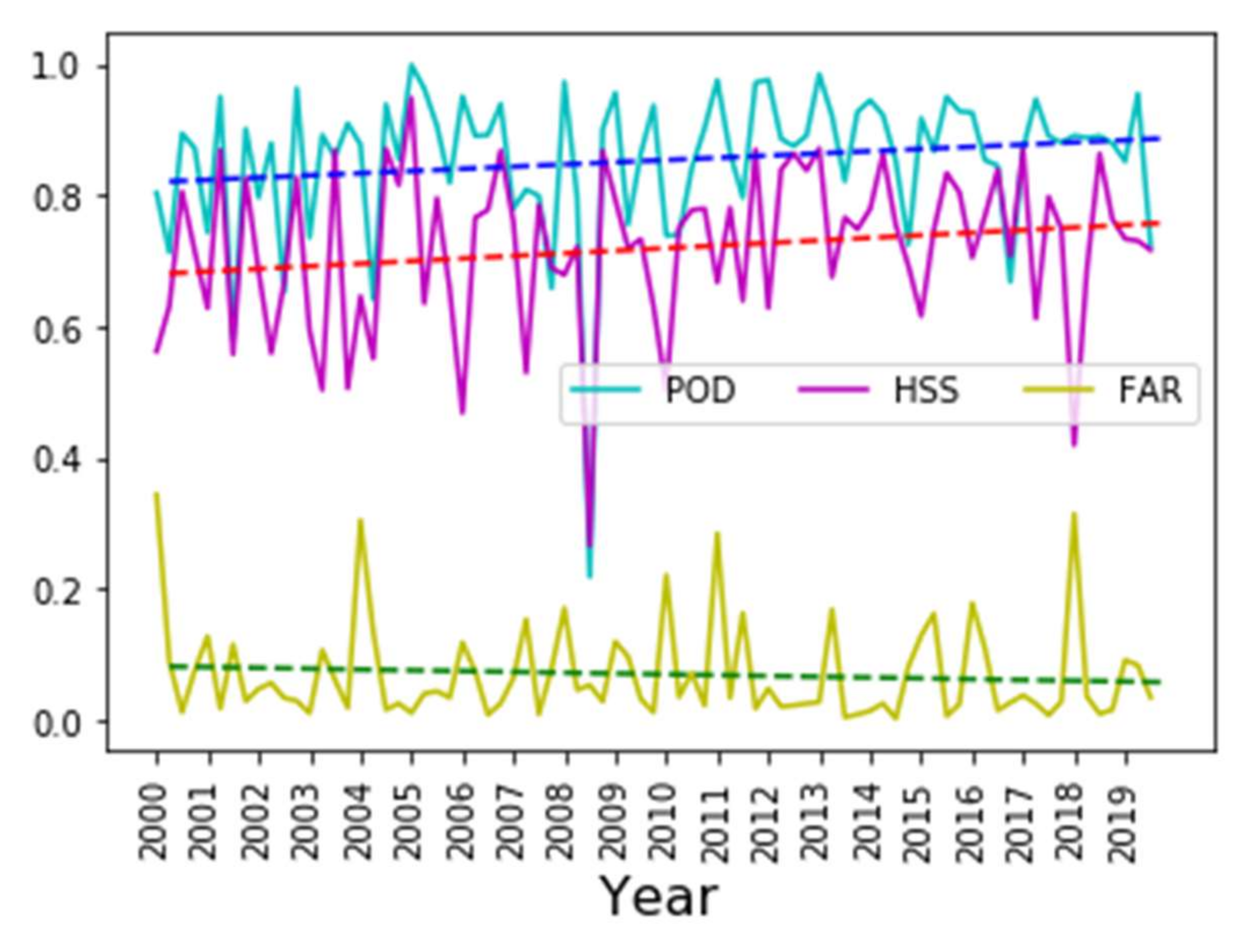
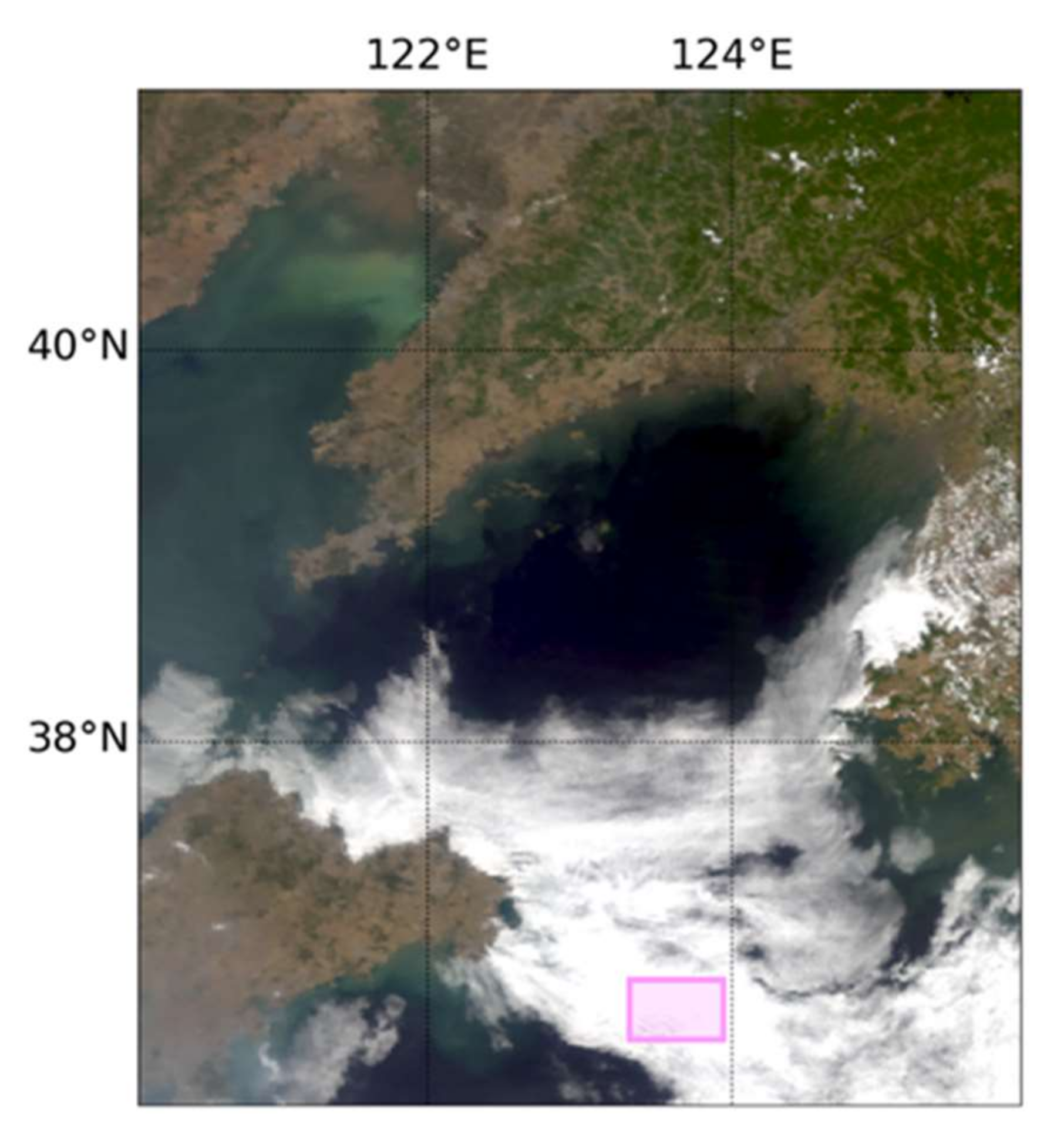
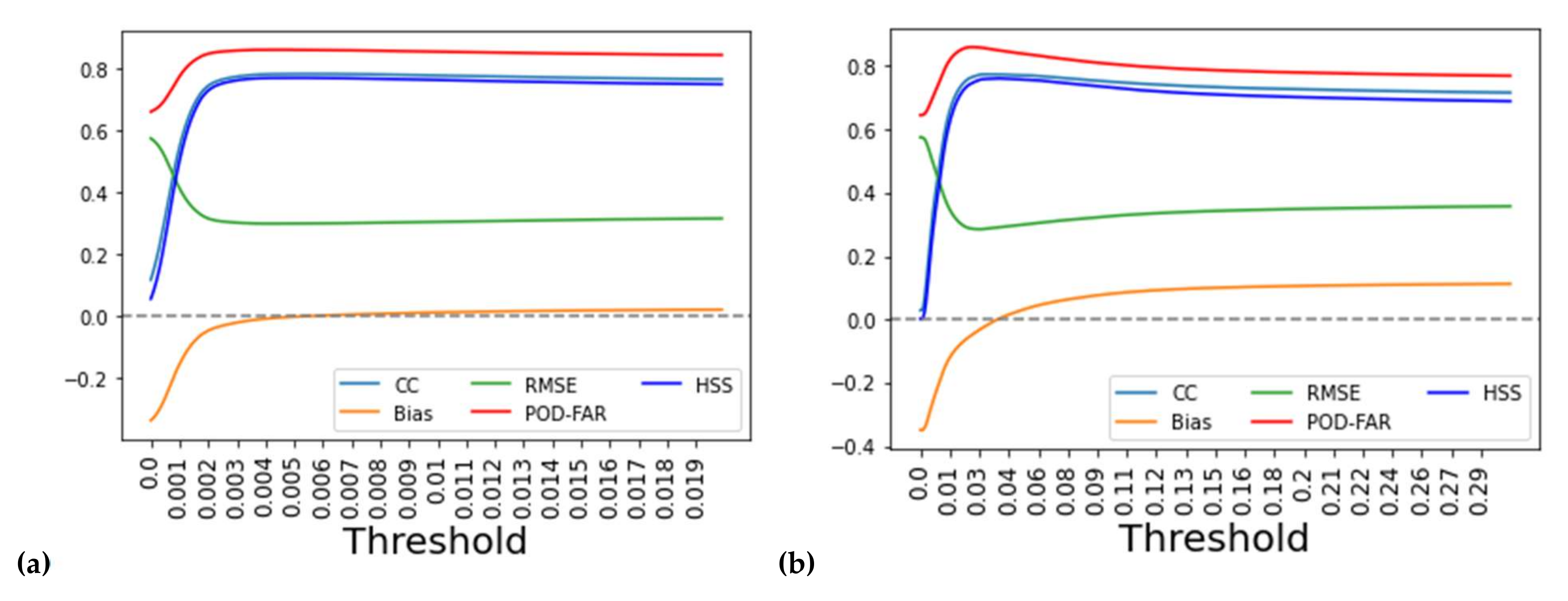
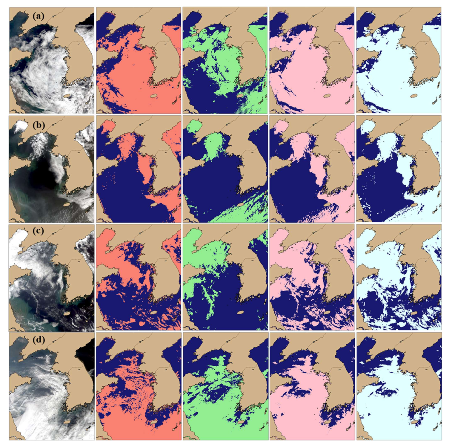
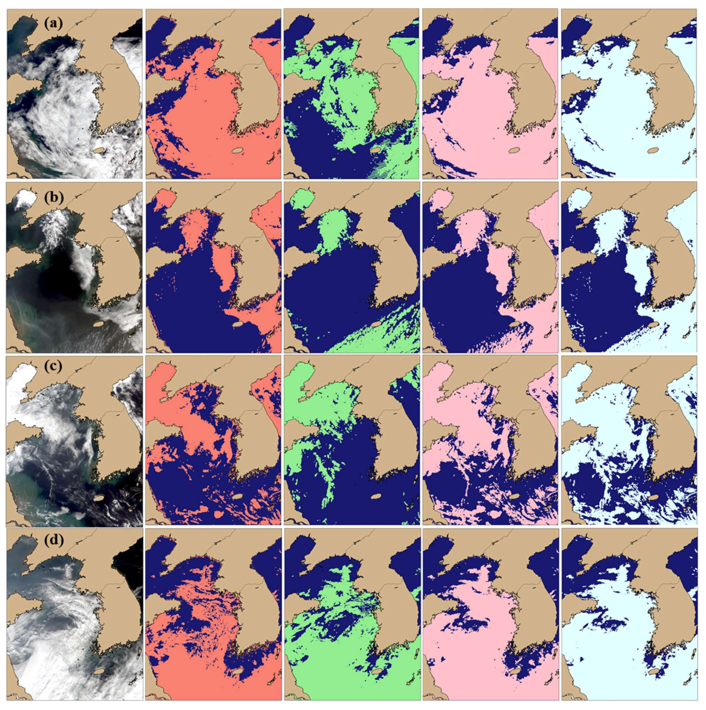
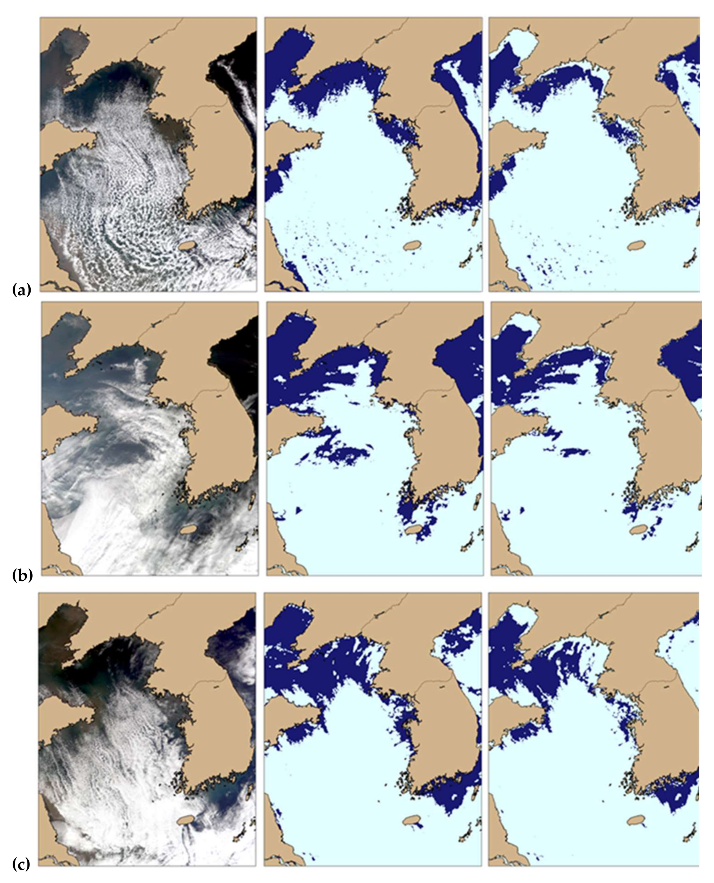
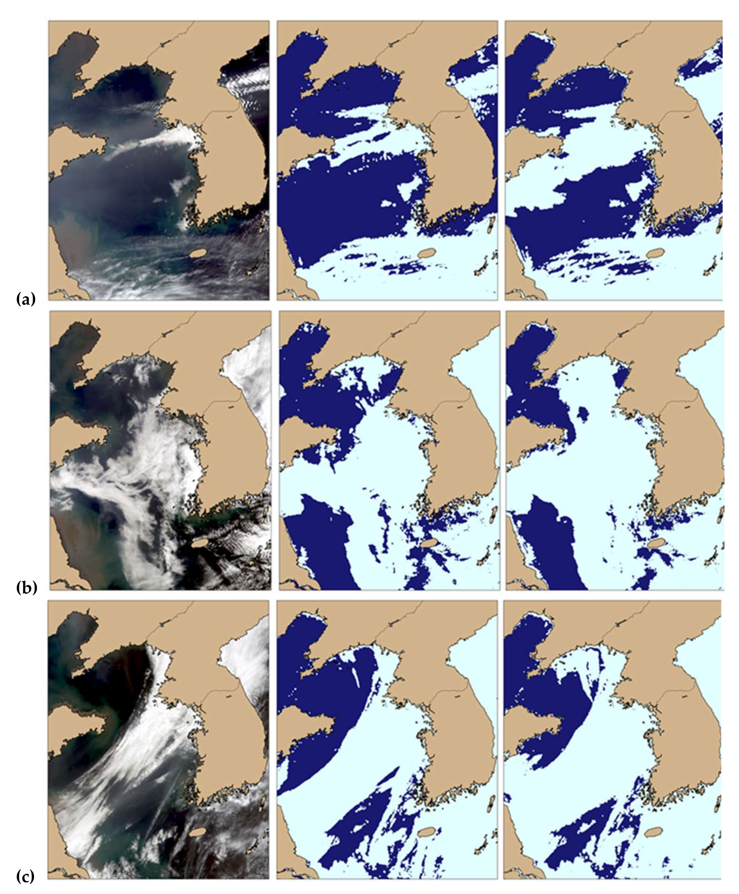
4. Results
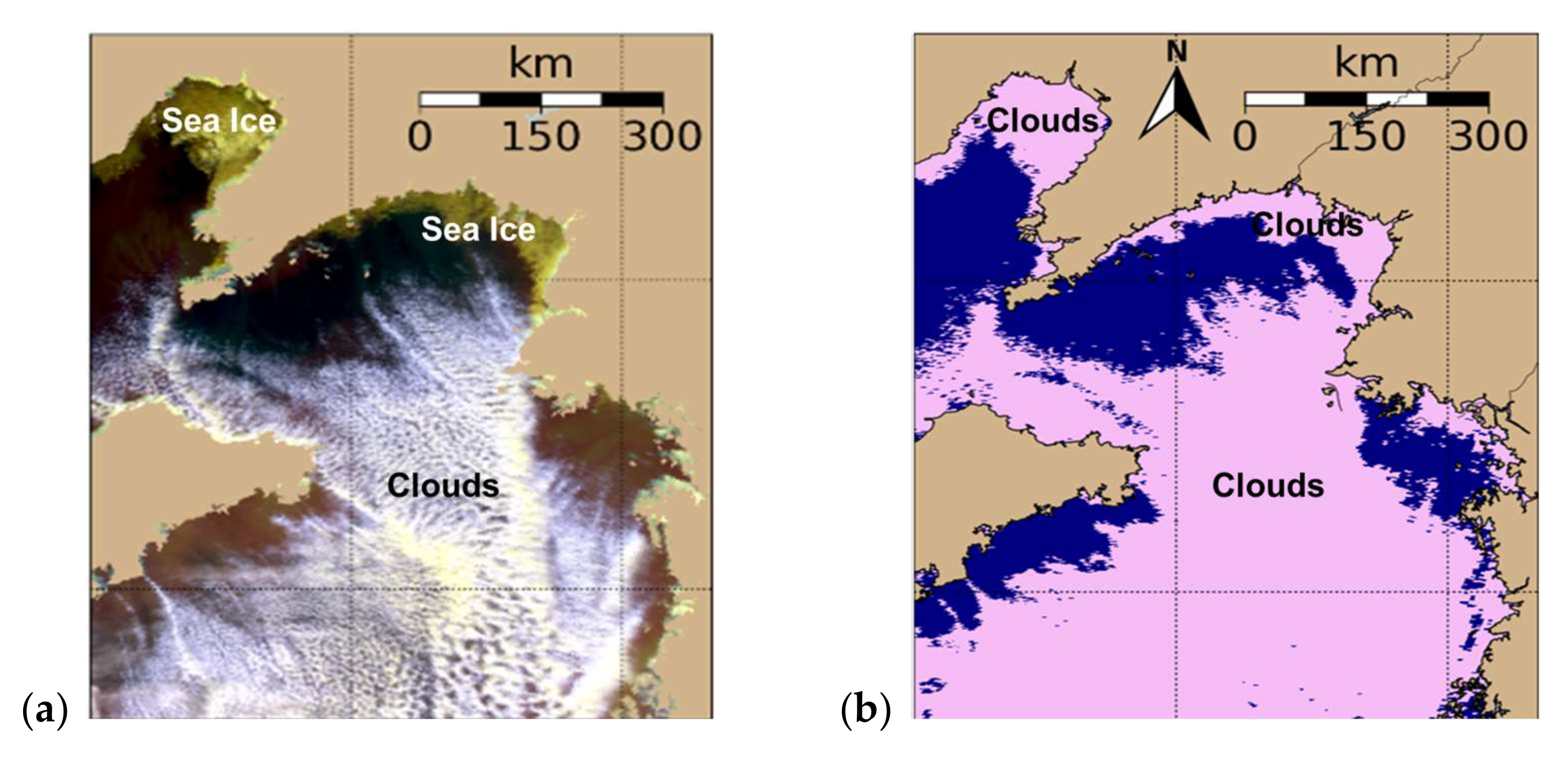
5. Discussion
6. Conclusions
Author Contributions
Funding
Data Availability Statement
Acknowledgments
Conflicts of Interest
References
- Stowe, L.; Vemury, S.; Rao, A. AVHRR clear-sky radiation data sets at NOAA/NESDIS. Adv. Space Res. 1994, 14, 113–116. [Google Scholar] [CrossRef]
- Xiang, H.-B.; Liu, J.-S.; Cao, C.-X.; Xuet, M. Algorithms for Moderate Resolution Imaging Spectroradiometer cloud-free image compositing. J. Appl. Remote Sens. 2013, 7, 073486. [Google Scholar] [CrossRef] [Green Version]
- Qiu, B.; Li, W.; Zhong, M.; Tang, Z.; Chen, C. Spatiotemporal analysis of vegetation variability and its relationship with climate change in China. Geo-Spat. Inform. Sci. 2014, 17, 170–180. [Google Scholar] [CrossRef] [Green Version]
- Zeng, Y.; Huang, W.; Zhan, F.B.; Zhang, H.; Liu, H. Study on the urban heat island effects and its relationship with surface biophysical characteristics using MODIS imageries. Geo-Spat. Inform. Sci. 2010, 13, 1–7. [Google Scholar] [CrossRef] [Green Version]
- Robinson, W.; Franz, B.A.; Frederick, S.P.; Bailey, S.; Werdell, J. Masks and flags updates. Algorithm updates for the fourth Sea-WiFS data reprocessing. NASA Tech. Memoran. 2003, 206892, 34–40. [Google Scholar]
- Wang, M.; Shi, W. Estimation of ocean contribution at the MODIS near-infrared wavelengths along the east coast of the US: Two case studies. Geophys. Res. Lett. 2005, 32, L13606. [Google Scholar] [CrossRef] [Green Version]
- Song, X.; Liu, Z.; Zhao, Y. Cloud detection and analysis of MODIS image. In Proceedings of the 2004 IEEE International Geoscience and Remote Sensing Symposium, Anchorage, AL, USA, 20–24 September 2004. [Google Scholar]
- Saunders, R.W.; Kriebel, K.T. An improved method for detecting clear sky and cloudy radiances from AVHRR data. Int. J. Remote Sens. 1988, 9, 123–150. [Google Scholar] [CrossRef]
- Zhu, Z.; Woodcock, C.E. Automated cloud, cloud shadow, and snow detection in multitemporal Landsat data: An algorithm designed specifically for monitoring land cover change. Remote Sens. Environ. 2014, 152, 217–234. [Google Scholar] [CrossRef]
- Ackerman, S.A.; Frey, R. MODIS Atmosphere L2 Cloud Mask Product (35_L2). NASA MODIS Adaptive Processing System, Goddard Space Flight Center, USA, 2015. Available online: https://modaps.modaps.eosdis.nasa.gov/services/about/products/c6/MOD35_L2.html (accessed on 23 September 2019). [CrossRef]
- Kraatz, S.; Khanbilvardi, R.; Romanov, P. A Comparison of MODIS/VIIRS Cloud Masks over Ice-Bearing River: On achieving consistent cloud masking and improved river ice mapping. Remote Sens. 2017, 9, 229. [Google Scholar] [CrossRef] [Green Version]
- Dorofy, P.; Nazari, R.; And, P.R.; Key, J. Development of a Mid-Infrared Sea and Lake Ice Index (MISI) using the GOES imager. Remote Sens. 2016, 8, 1015. [Google Scholar] [CrossRef] [Green Version]
- Chaouch, N.; Temimi, M.; Romanov, P.; Cabrera, R.; McKillop, G.; Khanbilvardi, R. An automated algorithm for river ice monitoring over the Susquehanna River using the MODIS data. Hydrol. Process. 2014, 28, 62–73. [Google Scholar] [CrossRef]
- Liu, H.; Zeng, D.; Tian, Q. Super-pixel cloud detection using hierarchical fusion CNN. In Proceedings of the 2018 IEEE Fourth International Conference on Multimedia Big Data (BigMM), Xi’an, China, 13–16 September 2018. [Google Scholar]
- Bulgin, C.E.; Mittaz, J.P.; Embury, O.; Eastwood, S.; Merchant, C.J. Bayesian cloud detection for 37 years of advanced very high resolution radiometer (AVHRR) global area coverage (GAC) data. Remote Sens. 2018, 10, 97. [Google Scholar] [CrossRef] [Green Version]
- Tan, K.; Zhang, Y.; Tong, X. Cloud extraction from Chinese high resolution satellite imagery by probabilistic latent semantic analysis and object-based machine learning. Remote Sens. 2016, 8, 963. [Google Scholar] [CrossRef] [Green Version]
- Fu, H.; Shen, Y.; Liu, J.; He, G.; Chen, J.; Liu, P.; Qian, J.; Li, J. Cloud detection for FY meteorology satellite based on ensemble thresholds and random forests approach. Remote Sens. 2019, 11, 44. [Google Scholar] [CrossRef] [Green Version]
- Ghosh, R.R.; Ali, M.S.; Hena, A.; Rahman, H. A simple cloud detection algorithm using NOAA-AVHRR satellite data. Int. J. Sci. Eng. Res. 2012, 3, 1–5. [Google Scholar]
- Li, C.; Ma, J.; Yang, P.; Li, Z. Detection of cloud cover using dynamic thresholds and radiative transfer models from the polarization satellite image. J. Quant. Spectrosc. Radiat. Transf. 2019, 222, 196–214. [Google Scholar] [CrossRef]
- Hagolle, O.; Huc, M.; Pascual, D.V.; Dedieu, G. A multi-temporal method for cloud detection, applied to FORMOSAT-2, VENµS, LANDSAT and SENTINEL-2 images. Remote Sens. Environ. 2010, 114, 1747–1755. [Google Scholar] [CrossRef] [Green Version]
- Zhu, Z.; Wang, S.; Woodcock, C.E. Improvement and expansion of the Fmask algorithm: Cloud, cloud shadow, and snow detection for Landsats 4–7, 8, and Sentinel 2 images. Remote Sens. Environ. 2015, 159, 269–277. [Google Scholar] [CrossRef]
- Murino, L.; Amato, U.; Carfora, M.F. Cloud detection of MODIS multispectral images. J. Atmos. Ocean. Technol. 2014, 31, 347–365. [Google Scholar] [CrossRef]
- Sun, L.; Mi, X.; Wei, J.; Wang, J.; Tian, X.; Yu, H.; Gan, P. A cloud detection algorithm-generating method for remote sensing data at visible to short-wave infrared wavelengths. ISPRS J. Photogramm. Remote Sens. 2017, 124, 70–88. [Google Scholar] [CrossRef]
- Stephens, G.L.; Vane, D.G.; Boain, R.J.; Mace, G.G.; Sassen, K.; Wang, Z.; Illingworth, A.J.; O’Connor, E.J.; Rossow, W.B.; Durden, S.L.; et al. The CloudSat mission and the A-Train: A new dimension of space-based observations of clouds and precipitation. Bull. Amer. Meteor. Soc. 2002, 83, 1771–1790. [Google Scholar] [CrossRef] [Green Version]
- Mao, F.; Duan, M.; Min, Q.; Gong, W.; Pan, Z.; Liu, G. Investigating the impact of haze on MODIS cloud detection. J. Geophy. Res. 2015, 120, 12237–12247. [Google Scholar] [CrossRef]
- Lee, K.H. 3-D perspectives of atmospheric aerosol optical properties over Northeast Asia using LIDAR on-board the CALIPSO satellite. Korean J. Remote Sens. 2014, 30, 559–570. [Google Scholar] [CrossRef]
- Platnick, S.; King, M.D.; Ackerman, S.A.; Menzel, W.P.; Baum, B.A.; Riédi, J.C.; Frey, R.A. The MODIS cloud products: Algorithms and examples from Terra. IEEE Trans. Geosci. Remote Sens. 2003, 41, 459–473. [Google Scholar] [CrossRef] [Green Version]
- Remer, L.A.; Kaufman, Y.; Tanré, D.; Mattoo, S.; Chu, D.; Martins, J.V.; Li, R.-R.; Ichoku, C.; Levy, R.C.; Kleidman, R.G.; et al. The MODIS aerosol algorithm, products, and validation. J. Atmos. Sci. 2005, 62, 947–973. [Google Scholar] [CrossRef] [Green Version]
- Ackerman, S.; Frey, R.; Strabala, K.; Liu, Y.; Gumley, L.; Baum, B.; Menzel, P. Discriminating Clear-Sky from Cloud with MODIS—Algorithm Theoretical Basis Document (MOD35). Products (MOD35). ATBD-MOD-06, 2010, 6.1, 121. Available online: http://modis-atmos.gsfc.nasa.gov/_docs/MOD35_ATBD_Collection6.pdf (accessed on 23 September 2019).
- Strabala, K. MODIS Cloud Mask User’s Guide. Available online: http://cimss.ssec.wisc.edu/modis/CMUSERSGUIDE.PDF (accessed on 23 August 2019).
- Frey, R.A.; Ackerman, S.A.; Liu, Y.; Strabala, K.I.; Zhang, H.; Key, J.R.; Wang, X. Cloud detection with MODIS. Part I: Improvements in the MODIS cloud mask for collection 5. J. Atmos. Ocean. Technol. 2008, 25, 1057–1072. [Google Scholar] [CrossRef]
- Ackerman, S.A.; Strabala, K.I.; Menzel, W.P.; Frey, R.A.; Moeller, C.C.; Gumley, L.E. Discriminating clear sky from clouds with MODIS. J. Geophys. Res. 1998, 103, 32141–32157. [Google Scholar] [CrossRef]
- Ackerman, S.; Holz, R.; Frey, R.; Eloranta, E.; Maddux, B.; McGill, M. Cloud detection with MODIS. Part II: Validation. J. Atmos. Ocean. Technol. 2008, 25, 1073–1086. [Google Scholar] [CrossRef] [Green Version]
- Thompson, J.A.; Paull, D.J.; Lees, B.G. An improved liberal cloud-mask for addressing snow/cloud confusion with MODIS. Photogramm. Eng. Remote Sens. 2015, 81, 119–129. [Google Scholar]
- Muhammad, P.; Duguay, C.; Kang, K.K. Monitoring ice break-up on the Mackenzie River using MODIS data. Cryosphere 2016, 10, 569. [Google Scholar] [CrossRef] [Green Version]
- Riggs, G.A.; Hall, D.K.; Ackerman, S.A. Sea ice extent and classification mapping with the Moderate Resolution Imaging Spectroradiometer Airborne Simulator. Remote Sens. Environ. 1999, 68, 152–163. [Google Scholar] [CrossRef]
- McFeeters, S.K. The use of the Normalized Difference Water Index (NDWI) in the delineation of open water features. Int. J. Remote Sens. 1996, 17, 1425–1432. [Google Scholar] [CrossRef]
- Gao, B.-C. NDWI—A normalized difference water index for remote sensing of vegetation liquid water from space. Remote Sens. Environ. 1996, 58, 257–266. [Google Scholar] [CrossRef]
- Rogers, A.; Kearney, M. Reducing signature variability in unmixing coastal marsh Thematic Mapper scenes using spectral indices. Int. J. Remote Sens. 2004, 25, 2317–2335. [Google Scholar] [CrossRef]
- Gao, B.-C.; Kaufman, Y.J. Selection of the 1.375-µm MODIS channel for remote sensing of cirrus clouds and stratospheric aerosols from space. J. Atmos. Sci. 1995, 52, 4231–4237. [Google Scholar] [CrossRef]
- Gao, B.-C.; Li, R.-R. Removal of thin cirrus scattering effects in Landsat 8 OLI images using the cirrus detecting channel. Remote Sens. 2017, 9, 834. [Google Scholar] [CrossRef] [Green Version]
- Meyer, K.; Yang, P.; Gao, B.-C. Optical thickness of tropical cirrus clouds derived from the MODIS 0.66 and 1.375-/spl mu/m channels. IEEE Trans. Geosci. Remote Sens. 2004, 42, 833–841. [Google Scholar] [CrossRef]
- Meyer, K.; Yang, P.; Gao, B.-C. Ice cloud optical depth from MODIS cirrus reflectance. IEEE Geosci. Remote Sen. Lett. 2007, 4, 471–474. [Google Scholar] [CrossRef]
- Gao, B.C.; Kaufman, Y.J.; Han, W.; Wiscombe, W.J. Corection of thin cirrus path radiances in the 0.4–1.0 μm spectral region using the sensitive 1.375 μm cirrus detecting channel. J. Geophys. Res. 1998, 103, 32169–32176. [Google Scholar] [CrossRef]
- Gao, B.-C.; Yang, P.; Han, W.; Li, R.-R.; Wiscombe, W.J. An algorithm using visible and 1.38-/spl mu/m channels to retrieve cirrus cloud reflectances from aircraft and satellite data. IEEE Trans. Geosci. Remote Sens. 2002, 40, 1659–1668. [Google Scholar]
- Meyer, K.; Platnick, S. Utilizing the MODIS 1.38 μm channel for cirrus cloud optical thickness retrievals: Algorithm and retrieval uncertainties. J. Geophys. Res. 2010, 115, D24209. [Google Scholar] [CrossRef]
- Wilks, D.S. Statistical Methods in the Atmospheric Sciences; Academic Press: Oxford, UK, 2011. [Google Scholar]
- Frey, R.A.; Ackerman, S.A.; Holz, R.E.; Dutcher, S.; Griffith, Z. The continuity MODIS-VIIRS cloud mask. Remote Sens. 2020, 12, 3334. [Google Scholar] [CrossRef]


| CMs | MODIS CM = 1 (Yes) | MODIS CM = 0 (No) |
|---|---|---|
| Proposed CM = 1 (Yes) | A | B |
| Proposed CM = 0 (No) | C | D |
| Year | Date | Purpose |
|---|---|---|
| 2000 | May 20 (03:00 UTC), July 27 (02:35 UTC), October 02 (03:05 UTC) | Test, Comparison |
| 2001 | January 01 (02:45 UTC), April 02 (02:25 UTC), July 05 (02:35 UTC), October 11 (02:20 UTC) | Test, Comparison |
| 2002 | January 08 (02:10 UTC), April 21 (02:15 UTC), July 03 (02:10 UTC), October 07 (02:10 UTC) | Test, Comparison |
| 2003 | January 02 (02:15 UTC), April 08 (02:15 UTC), July 07 (02:50 UTC), October 08 (02:20 UTC) | Test, Comparison |
| 2004 | January 01 (02:40 UTC), May 22 (02:50 UTC), July 22 (02:20 UTC), October 01 (02:25 UTC) | Test, Comparison |
| 2005 | January 01 (02:50 UTC), May 06 (02:20 UTC), July 09 (02:20 UTC), October 29 (02:20 UTC) | Test, Comparison |
| 2006 | January 15 (02:30 UTC), April 19 (02:45 UTC), July 15 (02:50 UTC), October 23 (02:25 UTC) | Test, Comparison |
| 2007 | January 04 (02:20 UTC), April 13 (02:50 UTC), June 25 (02:45 UTC), October 06 (02:50 UTC) | Test, Comparison |
| 2008 | January 03 (02:45 UTC), April 15 (02:50 UTC), July 26 (02:15 UTC), October 17 (02:45 UTC) | Test, Comparison |
| 2009 | January 02 (02:15 UTC), March 03 (02:40 UTC), July 29 (02:15 UTC), October 11 (02:50 UTC) | Test, Comparison |
| 2010 | January 05 (02:15 UTC), April 27 (02:15 UTC), August 11 (02:50 UTC), October 07 (02:45 UTC) | Test, Comparison |
| 2011 | January 06 (02:25 UTC), April 17 (02:45 UTC), August 27 (20:20 UTC), September 15 (02:50 UTC) | Test, Comparison |
| 2012 | January 02 (02:20 UTC), April 19 (02:45 UTC), August 25 (02:45 UTC), October 16 (02:20 UTC) | Test, Comparison |
| 2013 | January 04 (02:20 UTC), April 06 (02:45 UTC), June 06 (02:15 UTC), September 29 (02:45 UTC) | Test, Comparison |
| 2014 | January 07 (02:20 UTC), April 29 (02:20 UTC), July 11 (02:15 UTC), October 02 (02:45 UTC) | Test, Comparison |
| 2015 | January 06 (02:45 UTC), April 16 (02:20 UTC), June 12 (02:20 UTC), September 12 (02:40 UTC) | Test, Comparison |
| 2016 | January 06 (02:15 UTC), April 18 (02:20 UTC), August 08 (02:20 UTC), October 04 (02:15 UTC) | Test, Comparison |
| 2017 | June 01 (02:15 UTC) | Method development |
| January 11 (02:45 UTC), April 14 (02:15 UTC), July 10 (02:20 UTC), October 10 (02:45 UTC) | Test, Comparison | |
| 2018 | January 05 (02:50 UTC), April 04 (02:45 UTC), August 19 (02:40 UTC), October 06 (02:40 UTC) | Test, Comparison |
| 2019 | January 01 (02:45 UTC), April 07 (02:45 UTC), July 03 (02:50 UTC), October 04 (02:20 UTC) | Test, Comparison |
| Case | POD | FAR | HSS |
|---|---|---|---|
| 29 April 2014, 02:20 UTC | 0.984 | 0.010 | 0.903 |
| 12 June 2015, 02:15 UTC | 0.935 | 0.091 | 0.850 |
| 4 October 2019, 02:15 UTC | 0.950 | 0.010 | 0.943 |
| 6 January 2016, 02:15 UTC | 0.923 | 0.002 | 0.835 |
| Dates | CALIPSO vs. MODIS CM | CALIPSO vs. Proposed CM | ||||
|---|---|---|---|---|---|---|
| POD | FAR | HSS | POD | FAR | HSS | |
| Spring (25 March 2020) | 0.72 | 0.00 | 0.64 | 0.85 | 0.01 | 0.78 |
| Summer (15 July 2020) | 0.79 | 0.09 | 0.77 | 0.76 | 0.08 | 0.75 |
| Autumn (26 September 2020) | 0.91 | 0.05 | 0.91 | 0.89 | 0.03 | 0.91 |
| Winter (16 January 2021) | 0.97 | 0.06 | 0.70 | 0.97 | 0.02 | 0.84 |
Publisher’s Note: MDPI stays neutral with regard to jurisdictional claims in published maps and institutional affiliations. |
© 2022 by the authors. Licensee MDPI, Basel, Switzerland. This article is an open access article distributed under the terms and conditions of the Creative Commons Attribution (CC BY) license (https://creativecommons.org/licenses/by/4.0/).
Share and Cite
Choi, Y.-J.; Ban, H.-J.; Han, H.-J.; Hong, S. A Maritime Cloud-Detection Method Using Visible and Near-Infrared Bands over the Yellow Sea and Bohai Sea. Remote Sens. 2022, 14, 793. https://doi.org/10.3390/rs14030793
Choi Y-J, Ban H-J, Han H-J, Hong S. A Maritime Cloud-Detection Method Using Visible and Near-Infrared Bands over the Yellow Sea and Bohai Sea. Remote Sensing. 2022; 14(3):793. https://doi.org/10.3390/rs14030793
Chicago/Turabian StyleChoi, Yun-Jeong, Hyun-Ju Ban, Hee-Jeong Han, and Sungwook Hong. 2022. "A Maritime Cloud-Detection Method Using Visible and Near-Infrared Bands over the Yellow Sea and Bohai Sea" Remote Sensing 14, no. 3: 793. https://doi.org/10.3390/rs14030793
APA StyleChoi, Y.-J., Ban, H.-J., Han, H.-J., & Hong, S. (2022). A Maritime Cloud-Detection Method Using Visible and Near-Infrared Bands over the Yellow Sea and Bohai Sea. Remote Sensing, 14(3), 793. https://doi.org/10.3390/rs14030793