Abstract
Salinity in the Bering Sea is vital for the physical environment that is tied to the productive ecosystem and the properties of Pacific waters transported to the Arctic Ocean. Its salinity variability reflects many fundamental processes, including sea ice formation/melting and river runoff, but its spatial and temporal characteristics require better documentation. This study utilizes remote sensing products and in situ observations collected by saildrone missions to investigate Sea Surface Salinity (SSS) variability. All Satellite products resolve the large-scale pattern set up by the relatively salty deep basin and the fresh coastal region, but they can be inaccurate near the ice edge and near land. The SSS annual cycle exhibits seasonal maxima in winter to spring, and minima in summer to fall. The amplitude and timing of the seasonal cycle are variable, especially on the eastern Bering Sea shelf. SSS variability recorded by both saildrone, and satellite instruments provide unprecedented insights into short-term oceanic processes including sea ice melting, wind-driven currents during weather events, and river plumes etc. In particular, the Soil Moisture Active Passive (SMAP) satellite demonstrates encouraging skills in capturing the freshening signals induced by spring sea ice melting. The Yukon River plume is another source of intense SSS variability. Surface wind forcing plays an essential role in controlling the horizontal movement of plume water and thereby shaping the SSS seasonal cycle in local regions.
1. Introduction
The Bering Sea is a semi-enclosed, sub-arctic marginal sea in the North Pacific. Its bathymetry is almost equally divided by a deep basin and continental shelves. The eastern shelf is broad and stretches more than 500 km zonally and 1200 km meridionally (Figure 1). This contrasts with the narrow shelf (<100 km) in the west [1]. The eastern shelf has received considerable attention as it hosts intense interactions among ocean, ice, and atmosphere. The changing physical environment is capable of modulating the local ecosystem, which supports abundant seabirds and marine mammals as well as some of the United States’ most productive and commercially important fish species [2,3].

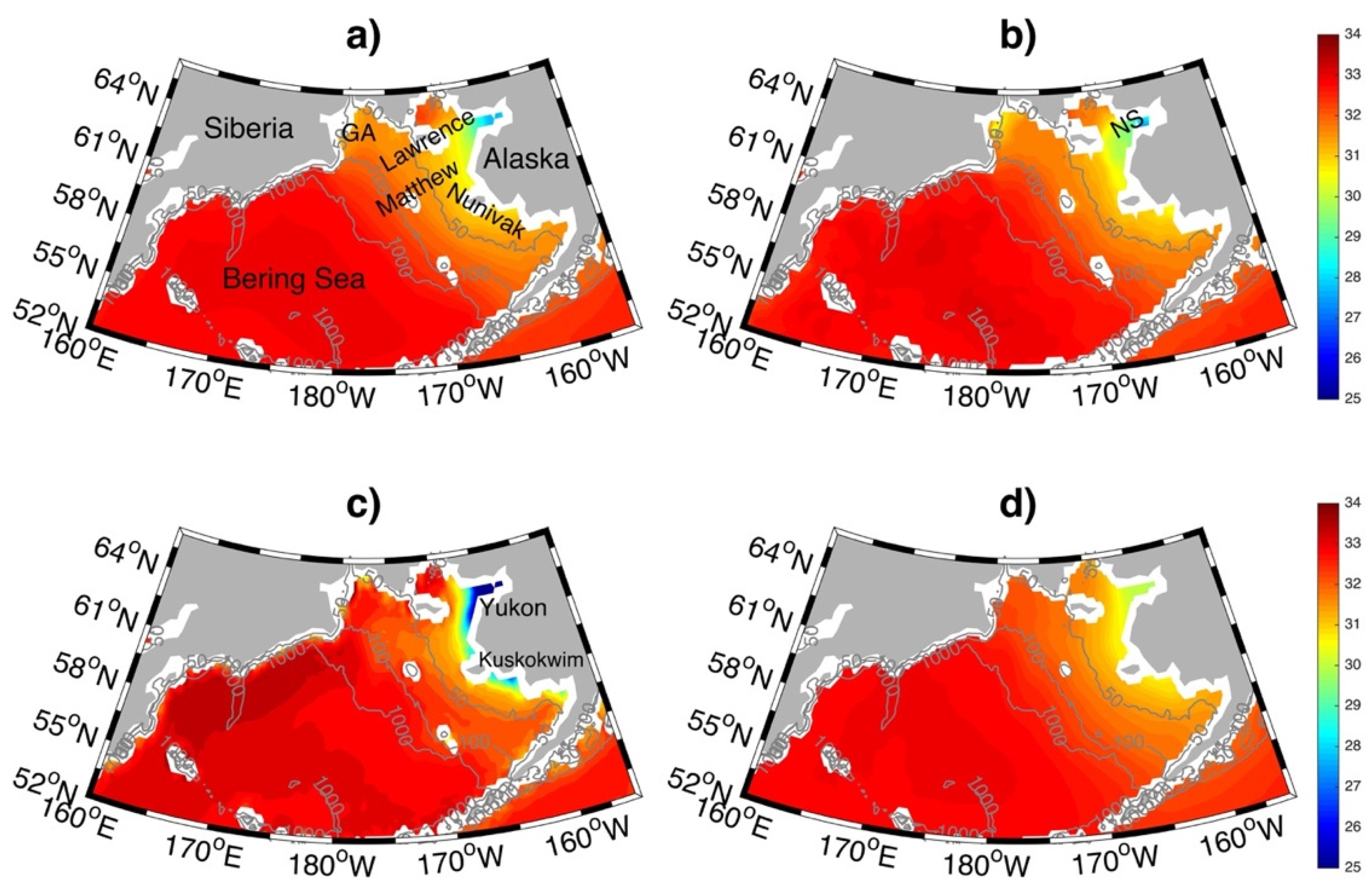
Figure 1.
Averaged Sea Surface Salinity in the Bering Sea in July 2015–June 2020 for CORA_OA (a), SMOS (b), SMAP (c) and OISSS (d). The isobaths of 50 m, 100 m and 1000 m are denoted in grey lines. Several important geographic locations are marked in panel (a): Gulf of Anadyr (GA); St. Lawrence Island (Lawrence); St. Matthew Island (Matthew); Nunivak Island (Nunivak). Panel (b) includes Norton Sound (NS). The locations for the mouths of the Yukon River and the Kuskokwim River are labelled in panel (c).
Salinity is an essential parameter in controlling the seawater properties over the eastern Bering Sea shelf, which directly mediates the transport of Pacific Water to the Arctic via the Bering Strait [4,5]. A freshening signal in the Bering Strait is expected to modify the vertical extent of Pacific Water in the Arctic [6]. Salinity also plays a key role in setting up the stratification and mixed layer depth in the shelf region. In the northern shelf (north of 60° N), salinity stratification is often as important as temperature stratification. On the southern shelf in summer, salinity can dominate stratification at sites on the inner shelf (≤50 m depth) and in regions of substantial prior ice-melt on the middle shelf (50–100 m depth), but temperature dominates at most middle-shelf locations [7,8].
The fundamental processes modulating salinity variability in the shelf region include seasonal ice formation-melting cycle and river runoff. Sea-ice cover is a defining characteristic for the Bering Sea. Despite the strong year-to-year fluctuations, sea ice normally starts to develop in the northern Bering Sea in November when the temperature drops to the freezing point (approximately −1.7 °C). Sea ice formed in the northern shelf advances southward under prevailing north-north-easterly winds [9,10]. Melting near the ice edge provides sizable freshwater to reduce the local salinity [11]. The maximum ice extent typically occurs in March and can cover almost the entire eastern shelf [12]. There are dramatic changes for the ice duration in the southern shelf where the seawater is often warmer than its freezing point. The spring melting and northward retreat of ice induce substantial salinity variability in the upper ocean [13,14]. In parallel, coastal river discharge becomes important in summer. The Yukon River and the Kuskokwim River are the major sources for freshwater, and their plumes create sharp salinity gradients [15,16,17,18]. With the breakdown of the inner front in late summer, this low-salinity signature spreads out over the shelf [19].
Our knowledge about the hydrography and salinity in the Bering Sea were mostly derived from shipboard samplings and moored measurements at single-point sites. However, the remoteness, ice coverage and harsh stormy weather limit the availability of in situ observations in winter and early spring. It is therefore difficult to construct a complete annual cycle for salinity over the vast shelf region. While moored instruments recorded temporal salinity changes associated with sea ice development [20,21], the corresponding spatial characteristics remain largely unknown. Moreover, the low salinity water near the ice edge has rarely been observed. These fresh lenses are expected to pose significant impacts on the air-sea exchanges of momentum and heat [22,23].
Remote sensing Sea Surface Salinity (SSS) observations became available since 2010 and offered unprecedented capability of mapping global SSS [24,25]. Current satellite missions, including Soil Moisture and Ocean Salinity (SMOS), Aquarius/SAC−D (Aquarius), and Soil Moisture Active Passive (SMAP), make use of L-band (1.4 GHz) microwave radiometry whose sensitivity is significantly reduced in cold temperatures. According to [26,27,28], the root-mean-square difference (RMSD) between SSS satellite data and in situ observation is about 1 PSS-78 [29] north of 50° N, which is much larger than the overall RMSD of 0.2 PSS-78 between 40° S and 40° N. Despite the uncertainties, remote sensing salinity was found to capture successfully the large salinity changes in the Arctic [30,31,32]. SSS averaged over the Arctic basin usually obtain encouraging results and the basin mean SSS displayed consistent annual and interannual variability with in situ products [32,33]. In addition, satellite salinity was also combined with ocean color data to quantify the river plume and infer a different freshwater source in the Arctic Ocean [34,35].
To evaluate remote sensing SSS in the Arctic Ocean and adjacent subpolar regions, it is necessary to pay attention to the intense near surface vertical salinity stratification [36]. Some in situ salinity observations might not be close enough to the surface and often yield large biases when validating L-band radiometric SSS, which are representative of the first top centimeter. Recently, Saildrone, Inc. uncrewed surface vehicles (USVs) have been widely deployed to make near-surface measurements in the Bering Sea, Chukchi Sea and Arctic Ocean [37,38]. The authors in [39] analyzed saildrone data in 2019 and the simultaneous remote sensing salinity products and concluded that many of the mesoscale-submesoscale variability were captured. Most importantly, they also pointed out SMAP products can resolve the marked salinity gradient near the Yukon River plume.
Many saildrone vehicles were launched from Dutch Harbor, AK and navigated through the eastern Bering Sea shelf. Some saildrones were designed to measure the eastern Bering Sea shelf [16,40,41]. These new observations augment traditional shipborne hydrographic casts and provide critical near-surface information. It is worth mentioning that the analysis of measurements in 2019 only covered a small part of the Bering Sea shelf [39]. This study presents saildrone observations in 2015–2017 when the shelf region is well sampled, aiming to document the synoptic variability of SSS. For the Bering Sea, winter sea ice had record-breaking low extent in recent years, exposing many regions to be sampled by satellite sensors. This study will take advantage of those winter surface salinity information in those usually ice-covered regions and derive a mean annual cycle in the Bering Sea.
2. Materials and Methods
2.1. In Situ Gridded Data
The gridded in situ salinity observations utilized in this study is the Coriolis Ocean dataset for ReAnalysis (CORA) created by the French Coriolis team. It is produced by a statistical objective analysis method developed and maintained at LOPS (Laboratoire d’Océanographie Physique et Spatial): the In Situ Analysis System (ISAS). The inputs are quality controlled in situ hydrographic profiles from different types of instruments: mainly Argo floats (including Ice Tethered Profiler), CTD, XBT and XCTD, sea mammals, moorings, drifting buoys, Thermosalinographs, and surface drifters, etc. [42,43]. This product is referred to as CORA_OA. Its salinity at 1 m depth is taken as SSS in this study. It is available on a monthly basis with horizontal grid spacing of 0.5°.
2.2. In Situ Saildrone Measurements
Several saildrones missions have been carried out in the Bering Sea and the Arctic since 2015 [16,40,41]. Some vehicles targeted the Arctic region and therefore did not spend much time in the Bering Sea. This study selected the vehicles and missions that mostly surveyed the eastern Bering Sea shelf in 2015, 2016 and 2017. Different types of instruments were installed to collect variables required to quantify air-sea fluxes, including air temperature, humidity, wind speed and direction, ocean temperature and salinity, etc. While both temperature and salinity reflect ocean properties, most saildrones missions began in spring and finished in summer. The overwhelming signal in the observed temperature data is gradual warming from spring to summer with an increase of about 6–10 °C. Surface heating in summer is widely distributed and yield warming signals in the entire Bering Sea shelf. Consequently, it is very challenging to infer water mass distributions based on near surface temperature only. In contrast, salinity demonstrate more regionally dependent variations, making it a good indicator for ocean dynamics. Thus, our analysis only involves salinity recorded by the Teledyne RDI Citadel CTD. The nominal measurement depth is 0.5 m or 1 m.
In 2015, saildrone vehicle sd-128 rendezvoused with the NOAA ship, Oscar Dyson, three times between 1 and 10 May 2015 for instrument comparisons [16,40]. The ship data were collected at 2.5 m depth and saildrone measurements were at 0.5 m. Their maximum difference was less than 0.1 PSS-78 and the rms difference was about 0.01 PSS-78 [16]. No inter-comparison was carried out in other years. However, there were at least two vehicles deployed in each year and they had crossovers or approached each other (less than 1 km). Salinity records during those crossing periods were selected. Their comparisons display good agreement with difference ranging from 0.03 PSS-78 to 0.1 PSS-78 and rms difference of 0.02 PSS-78. Thus, salinity observations from saildrones were assumed to be of good quality. We also notice that some saildrone vehicles had CTDs installed in keel tunnel where the flow was unpumped, relying on the speed of saildrone through the water to push water through the tunnel. Our quality control analysis indicates that this likely induces salinity bias of about 0.02 PSS-78 and also as large as 0.3 PSS-78 at few moments. However, those errors have little impact on our analysis as we mostly spatially average the saildrone measurements over more than 10-km to match with satellite data.
2.3. Satellite SSS Products
Three remote sensing SSS products were analyzed, which were created by different quality control processes. The first one is SMAP product from Remote Sensing Systems Version 4.0 (referred as SMAP hereafter). SMAP dataset is a level 3 product with 8-day running mean [44]. Its processing produces gridded data with feature resolution at both 40 km (RSS40 km) and 70 km (RSS70 km). It is available from May 2015 to present on a 0.25° × 0.25° daily grid. Both are utilized for comparison with the saildrone data, which yield quite similar statistical results including mean difference and standard deviation of difference. However, RSS40 km often displays nosier spatial pattern near the 50 m isobath and coastline. Here only the RSS70 km is presented.
The second one is SMOS level 3 debiased version-5 dataset produced by LOCEAN/IPSL (UMR CNRS/UPMC/IRD/MNHN) laboratory and ACRI-st company that participate in the Ocean Salinity Expertise Center (CECOS) of Centre Aval de Traitement des Donnees SMOS (referred as SMOS hereafter). It is provided by 9-day running mean maps on an Equal-Area Scalable Earth (EASE) 25-km grid. It spans from January 2010 to November 2020 every four days [45].
The third is Multi-Mission Optimally Interpolated Sea Surface Salinity (OISSS) Level 4 V1.0 dataset (referred as OISSS hereafter). This dataset maps the Level-2 orbital swath data from the AQUARIUS/SAC-D mission (25 August 2011 to 7 June 2015), the Soil Moisture Active Passive (SMAP) mission (April 2015-present) and Soil Moisture and Ocean Salinity (SMOS) mission onto a 0.25° spatial and 4-day temporal grid using Optimal Interpolation (OI). The two-month overlap between Aquarius and SMAP was used to ensure consistency and continuity in the data record. SMOS data were used only to fill the SMAP data gap during 19 June–24 July 2019, when SMAP satellite was in a safe mode [46].
Monthly average fields are also constructed for the three satellite products. For each individual grid point, its monthly mean is calculated only when the valid data points within that month cover at least 20 days in the original time series. The resulting monthly data are further used to construct 12 climatological fields to study the annual cycle.
2.4. Surface Wind
Winds are extracted from the National Center for Environmental Prediction (NCEP) North American Regional Reanalysis (NARR) model hindcasts [47]. The NARR reanalysis dataset includes surface pressure, wind, temperature and ocean-atmosphere heat fluxes every three hours. Here, only the daily mean winds are utilized to match the satellite maps. Its spatial resolution is about 32-km. This wind field was selected to examine the relationship between wind and ocean velocity in the eastern Bering Sea shelf [48].
3. Results
3.1. SSS in Gridded Datasets
3.1.1. Mean SSS Fields
The mean states of SSS are obtained by averaging the available data from CORA_OA, SMOS, SMAP and OISSS between July 2015 and June 2020. The four products agree broadly in the overall SSS spatial structure in the deep basin of the Bering Sea (Figure 1). SSS in the deep ocean is around 33 PSS-78 with maximum values in the central basin. Their similarity is also confirmed by the relatively small differences (less than 0.2 PSS-78) in regions deeper than 1000 m (Figure 2). Notable discrepancy occurs in the north-western Bering Sea, where SMAP is larger than CORA_OA by more than 1 PSS-78 off the east coast of Siberia. This is likely due to land contamination as differences arise near the land.
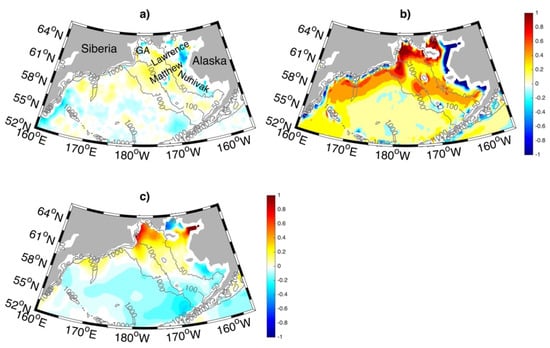
Figure 2.
Difference of mean Sea Surface Salinity between CORA_OA and the other three satellite products: SMOS minus CORA_OA (a); SMAP minus CORA_OA (b); OISSS minus CORA_OA (c). The isobaths of 50 m, 100 m and 1000 m are in grey lines.
The most striking feature in the eastern Bering Sea shelf is the low salinity water in the Norton Sound that receives the Yukon River discharge (Figure 1). Along 165°W near the center of Norton Sound, the lowest value in mean SSS is about 25–26 PSS-78 in SMAP, 28–29 PSS-78 in CORA_OA and SMOS, and 30 PSS-78 in OISSS. Those numbers are in line with their differences shown in Figure 2. Note that there is intense salinity front associated with the river plume [39]; it is not a surprise to find significant biases in gridded datasets.
SMAP data also reveals that low salinity waters extend southward along the coast of Alaska (Figure 1c). This feature seems to be reasonable considering the freshwater input from the Kuskokwim River. However, none of the other three datasets capture these coastal low salinity values. The Gulf of Anadyr is another region with high disparity among the datasets, with SSS in SMAP and OISSS higher than CORA_OA by more than 1 PSS-78.
The overall SSS variations are quantified by standard deviation (STD). Gulf of Anadyr and Norton Sound are hotspots for the elevated variability (STD > 1) due to sea ice formation/melting and river discharges (Figure 3). OISSS displays much lower STD over there, suggesting that more realistic signals are excluded in its quality control process. There are also remarkable variabilities around St. Lawrence Island and Nunivak Island, but they are only pronounced in SMAP. They are not necessarily bias as dramatic salinity changes were documented in this area [8,17,21]. In contrast, SMAP also includes high STD along the east coast of Siberia, which is very likely to be uncertainties/errors near the land.
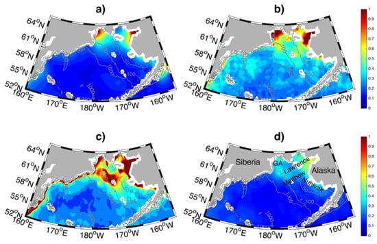
Figure 3.
Standard deviation fields for CORA_OA (a), SMOS (b), SMAP (c) and OISSS (d). The isobaths of 50 m, 100 m and 1000 m are in grey lines.
3.1.2. Annual Cycle
To illustrate the annual cycle, monthly mean SSS fields in March, June, September, and December are extracted from the four datasets over the period of July 2015 to June 2020 (Figure 4). These four months are selected to represent the typical maximum sea ice extent (March), early summer (June), fall (prior to ice formation, September) and early winter (developing stage of ice formation, December) in the eastern Bering Sea shelf. Because of sea ice, remote sensing SSS in winter are usually inaccessible over a large proportion of the eastern Bering Sea shelf. However, the record-breaking low sea ice extent in 2018 and 2019 enabled much more ice-free regions to be recorded in satellite data [12]. To obtain more robust results, the monthly fields in Figure 4 include at least two valid data points at each grid. Note that SSS from satellites are the salinity in the uppermost skin layers and they should be different from the near surface salinity in the presence of sea ice.
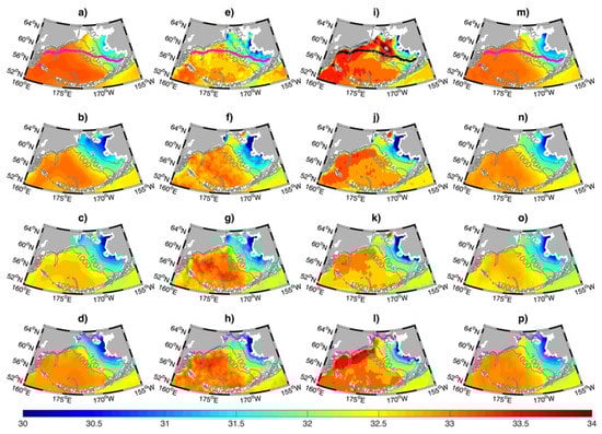
Figure 4.
Monthly mean SSS produced from CORA_OA (a–d), SMOS (e–h), SMAP (i–l) and OISSS (m–p) in March (first row), June (second row), September (third row), and December (bottom row). The isobaths of 50 m, 100 m and 1000 m are marked by grey lines. Magenta and black (in panel i) lines are the maximum sea ice edge during 2015–2020. Note, white area in the top row (a,e,i,m) is missing data due to ice.
The region north of St. Lawrence Island is mostly masked by sea ice in March (Figure 4). Fresher waters are found along the Alaskan coast and serve to maintain large-scale horizontal gradients between the eastern shelf and deep ocean. Inter-comparisons between the four datasets reveal their distinct characteristics. The coastal salinity in CORA_OA is apparently higher than those from the other three products (Figure 4a). SMOS displays lower SSS in the Gulf of Anadyr (Figure 4e). SSS near St. Matthew Island are much higher (by more than 1 PSS-78) in SMAP (Figure 4i). By June low salinity waters spread to the central shelf. They mainly stay in the inner shelf (<50 m isobath) in SMOS, SMAP and OISSS (Figure 4f,j,n). In contrast, they also extend to Gulf of Anadyr in CORA_OA (Figure 4b). SSS patterns in September are similar to those in June. The most noticeable changes exist in Gulf of Anadyr where SSS increases in CORA_OA (Figure 4c) and decreases in SMOS (Figure 4g). The coastal freshwater retreats in December but remains fresher than March in the four products.
One distinct feature for SSS over the shelf region is the parallel between isohalines and isobaths. This applies to all products and all seasons. Such behavior results from the fact that their spatial patterns are largely shaped by oceanic advective salinity changes. Any salinity anomalies, either due to sea ice melting or river discharge, are spread by ocean currents whose directions are mostly guided by isobaths [1,4].
SSS changes in the deep ocean are relatively weaker. They are visually lower in September than March for CORA_OA, SMAP and OISSS. In contrast, SMOS displays an opposite trend, in which deep-basin SSS is lower in March than in September (Figure 4e,g). The positive biases off the east coast of Siberia in SMAP persist throughout the year, suggesting that they are affecting the entire dataset rather than certain periods (Figure 4i–l).
The maximum and minimum of the annual cycle are taken as average of the topmost 5% and lowest 5% values, respectively, over 2015–2020 from the four products. This approach is to reduce the uncertainty due to noises in satellite data and some accidental influencing factors. The difference between maximum and minimum are defined as the amplitude for the seasonal SSS variability. The overall patterns for the amplitudes are similar to the STD fields in Figure 3, indicating that substantial variability takes place on the seasonal time scale. Gulf of Anadyr carries the largest amplitude (Figure 5). It is more than 2 PSS-78 for CORA_OA, SMOS and SMAP, but is only about 0.8 PSS-78 in OISSS. Large values are also found around St. Matthew Island in SMOS and SMAP. The peak-to-peak ranges in deep ocean are quite weak (~0.2–0.3 PSS-78) in CORA_OA and OISSS. SMOS and SMAP, however, exhibit much noise in the deep ocean and their amplitude can reach up to 0.7–0.8 PSS-78 in some regions.
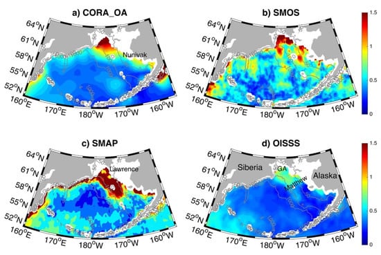
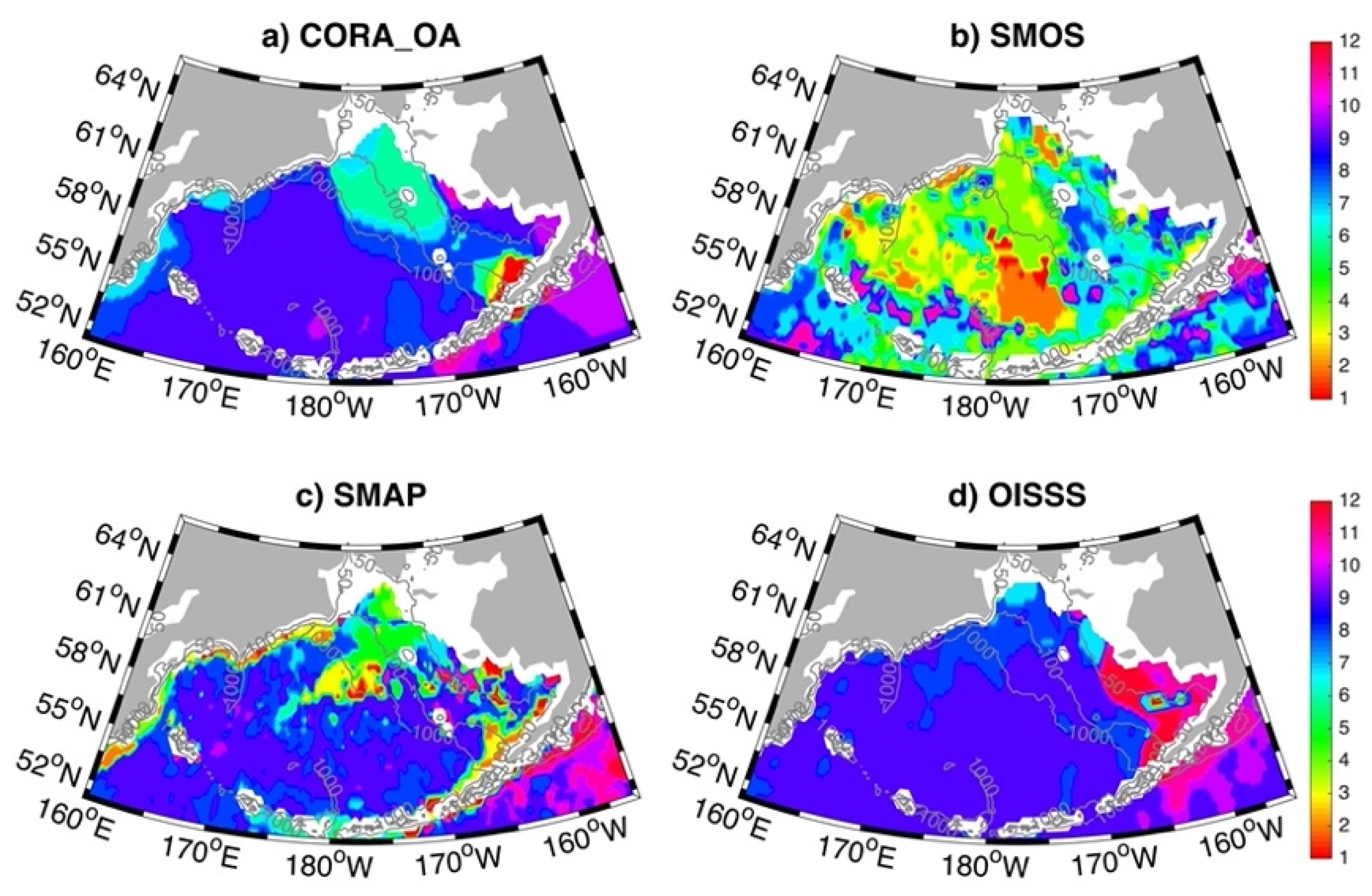
Figure 5.
Amplitude (maximum minus minimum) for the sea surface salinity annual cycle in CORA_OA (a); SMOS (b); SMAP (c) and OISSS (d). The annual cycle is extracted using monthly data in July 2015–June 2020. Grey lines indicate isobaths of 50 m, 100 m, and 1000 m. Note, white area is missing data.
Timings for the maximum and minimum of SSS are also extracted for the annual cycle. The maximum mostly arises in winter for CORA_OA, SMAP and OISSS (Figure 6). For instance, it is either March or April in the eastern Bering Sea shelf (<100 m). Though appearing patchy in the deep ocean, it mainly ranges from January to April. SMOS, on the contrary, has its maximum in October and November in both the eastern shelf and deep ocean. The minimum in the four datasets is frequently identified from June to September, which is likely associated with sea ice melting and river discharge (Figure 7). There are a few exceptions, including November–December in the inner shelf in OISSS, and January–March in the deep ocean in SMOS. Such localized patterns in the particular timings of seasonal maximum and minimum indicate that there are considerable variabilities imposed upon the annual cycle. The following section will demonstrate that SSS synoptic changes are rich in the eastern Bering Sea shelf.
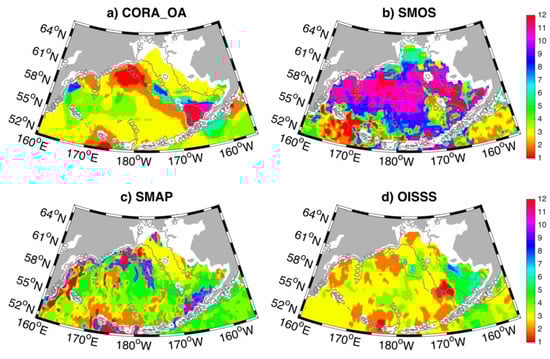
Figure 6.
The maximum value of the sea surface salinity annual cycle in CORA_OA (a); SMOS (b); SMAP (c) and OISSS (d). The annual cycle is extracted using monthly data in July 2015–June 2020. Grey lines indicate isobaths of 50 m, 100 m, and 1000 m. Note, white area is missing data.
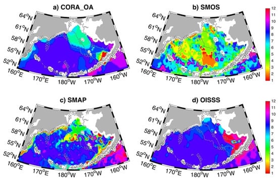
Figure 7.
Similar to Figure 6, but for the minimum value of the sea surface salinity annual cycle in CORA_OA (a); SMOS (b); SMAP (c) and OISSS (d). Note, white area is missing data.
3.2. SSS during Saildrone Missions
Saildrone observations are time series along the trajectories of vehicles. To match them with gridded satellite data, we adopted the collocation method by Vazquez-Cuervo et al. [39] to interpolate the one-minute saildrone measurements to the nearest grids in each satellite dataset. For each unique gridded satellite data point, all matched saildrone data were averaged within that grid cell, providing a single matchup saildrone data point for each single satellite retrieval. CORA_OA, SMAP and OISSS share the same 0.25° grid and their matchups procedures are thus identical. SMOS has different grid and spatial resolution of 25 km, which is about 1/3° in the Bering Sea region. However, each selected grid cell in satellite products usually has hundreds of matched data points from saildrone data and their average shows negligible difference between 0.25° and 1/3° resolution datasets.
More than one saildrone was deployed in each year. They operated simultaneously but did not necessarily follow identical tracks. Statistical comparisons between each individual saildrone mission and three satellite products were evaluated using three metrics: correlation, bias (satellite minus saildrone) and Root Mean Square of the Difference (RMSD). The correlation reflects how well satellite data resolve the spatial gradients of SSS. Its confidence level was performed assuming Student’s t test at 95%. Most satellite products are significantly correlated with paired saildrone data (Table 1). The only exception is SMOS and OISSS data in 2016. As shown below, saildrone vehicles, SD126 and SD128, in 2016 mostly stayed in the southern shelf where salinity spatial gradients were quite weak. All satellite datasets exhibit positive biases with respect to saildrone data. Higher biases are normally accompanied with larger values of RMSD, indicating that satellite products have better performance in some area, but evidently degrades in other regions. Their detailed performance is discussed in the following.

Table 1.
Statistical comparison between saildrone data and satellite products. Saildrone missions are listed in the first column where vehicle name begins with SD and the survey year is underneath. Metrics for evaluation include correlation (95% confidence level in parentheses), Bias and Root Mean Square of the Difference (RMSD).
3.2.1. Saildrone Missions in 2015
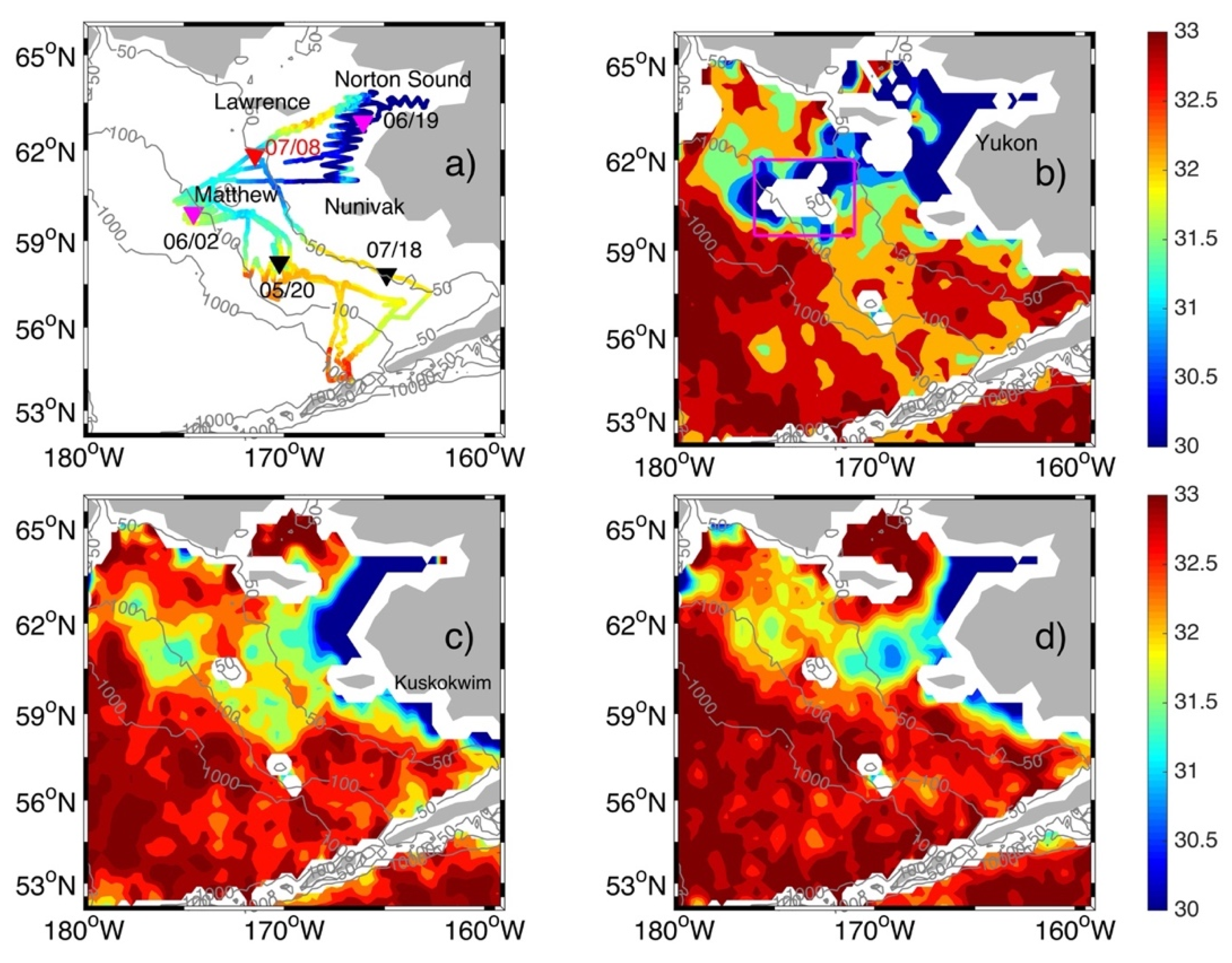
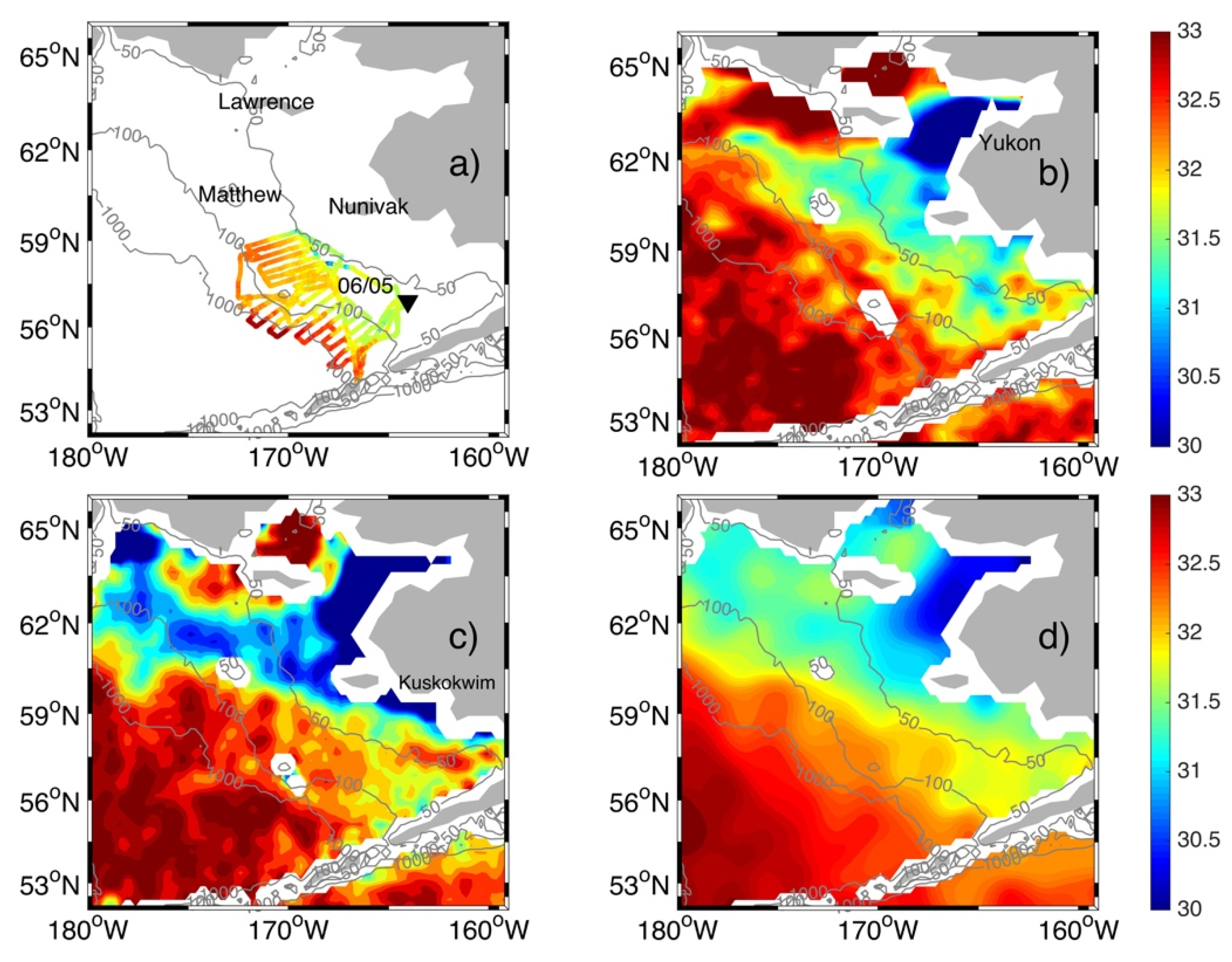
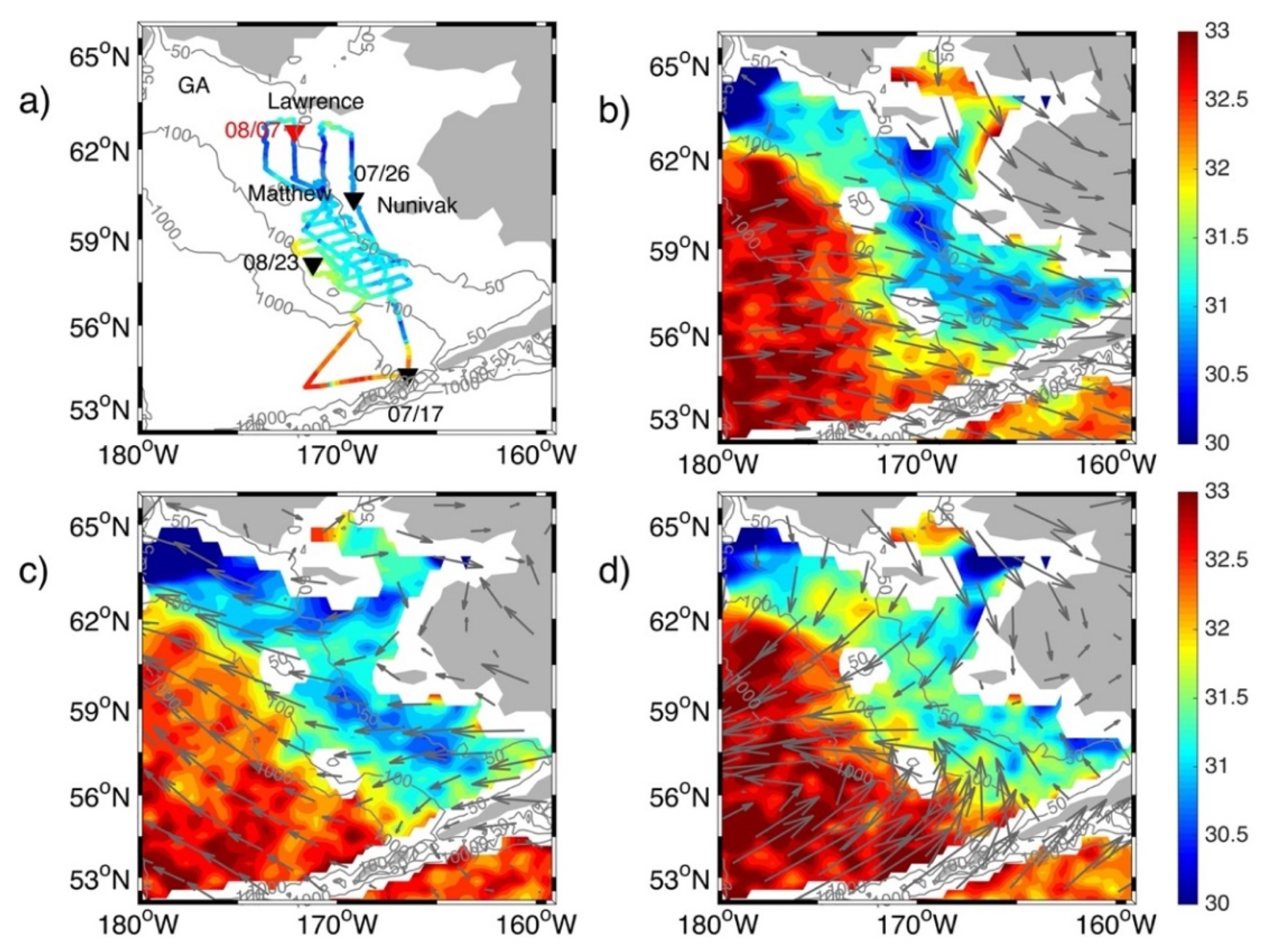
Two saildrone vehicles SD126 and SD128 were launched at Dutch Harbor, AK in April 2015 to survey the eastern Bering Sea shelf [16,40]. They navigated northward near the isobaths of 70 m and 100 m (Figure 8a). They were programmed to sample the oceanographic fields following sea ice melting near St. Matthew Island and also observe the Yukon River plume. On 20 May 2015 when both vehicles were still south of 59°N, SMAP data displayed freshwater encircling the sea ice margin near St. Matthew Island (Figure 8b). The observed freshwater was a typical feature for the melt water. Saildrones approached the Island in early June when the surrounding SSS increased to about 31–31.5 PSS-78. Such an increase likely resulted from vertical mixing induced by winds. The 31.5 isohaline is usually taken as an indicator for the melt-water edge [8]. Both saildrone and SMAP data captured this lens of freshwater in the vicinity of St. Matthew Island (Figure 8a,c).
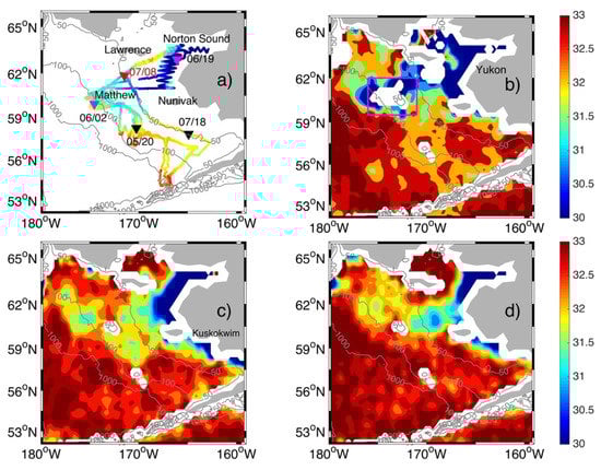
Figure 8.
(a) In situ salinity (color shading) from saildrone vehicles 126 and 128 along their trajectories. The launch site is the southern end of their tracks and time span is 26 April to 28 July 2015. Passing time (month/day) for a few spots (triangles) are provided as reference. Snapshots for SSS are extracted from SMAP products on 20 May (b), 2 June (c) and 12 July (d). Note, white area is missing data.
The vehicles reached the Yukon River plume in mid-June and followed a sawtooth course near the salinity front. During this period, coastal freshwater widely was distributed from the Yukon River mouth (Norton Sound) to 56°N (about Bristol Bay). These waters mostly stay in shallow regions (less than 30 m or 20 m). The saildrones started to return in early July along the isobath of 50 m. The Yukon River plume retreated, but a lens of freshwater resided east of St. Matthew Island and near the 50 m isobath (Figure 8d).
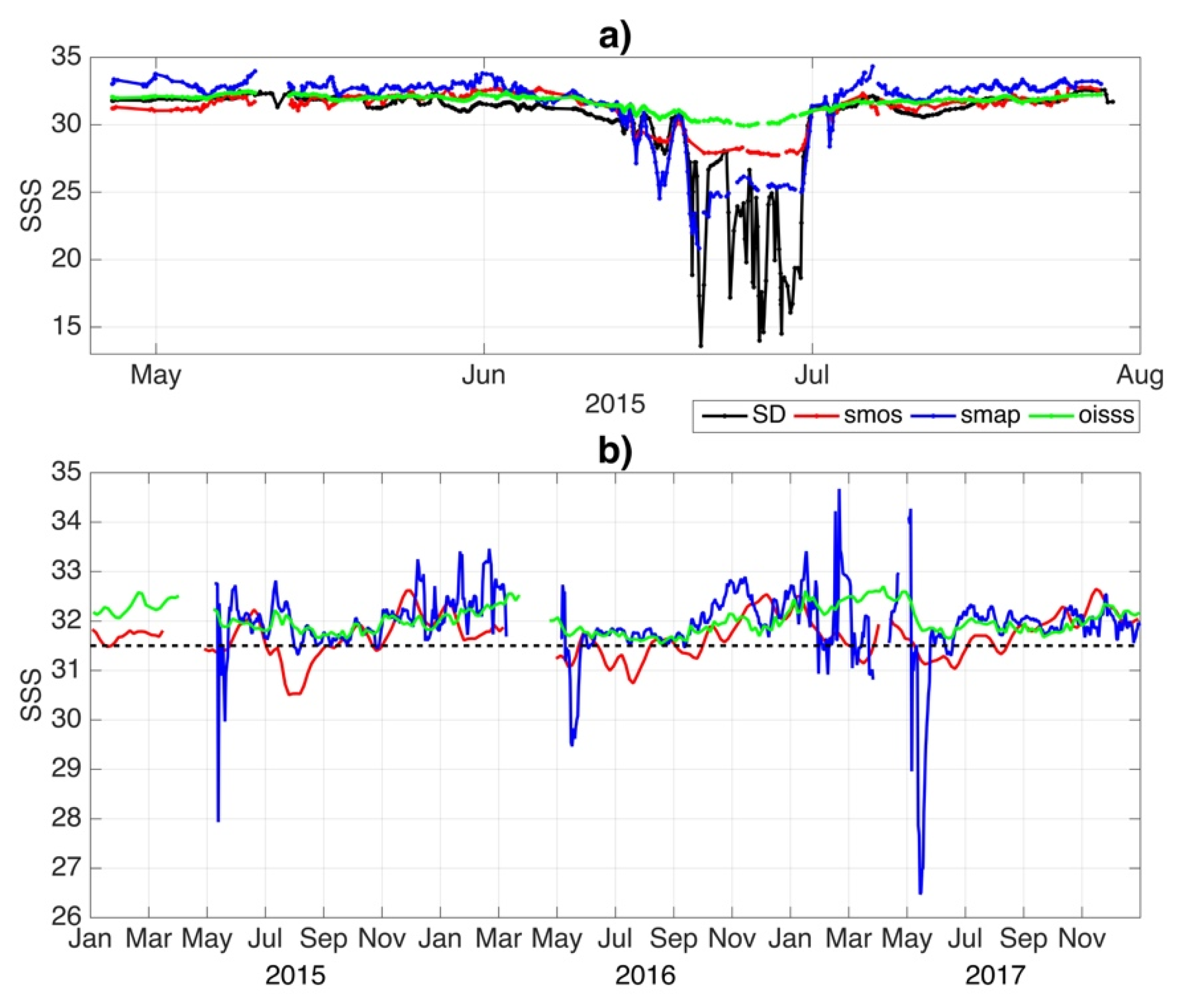
The point-to-point comparison between satellite data and saildrone SD128 measurements reveal both temporal and spatial SSS variability along saildrone’s track (Figure 9a). SSS from all datasets is relatively stable in May although SMAP displays general overestimation. They start to decrease in early June when the vehicle approached St. Matthew Island. Saildrone recorded further lower SSS values (less than 25 PSS-78) in mid-June when it was near the Yukon River plume. The large amplitude fluctuations in SSS clearly demonstrate the sharp SSS spatial gradient when the vehicle moved back-and-forth near the plume. SMAP exhibits the best performance as it exactly captures the initial transition from high SSS (>30 PSS-78) to low SSS (<25 PSS-78). SMAP data is quite stable thereafter because its temporal resolution is much coarser than the rapidly moving saildrone vehicles. Nevertheless, SMAP still shows a statistically high correlation with saildrone data (Table 1). In contrast, OISSS completely fails to resolve the plume regime. SMOS seems to capture the salinity front, but its SSS in the near coast is much higher than that recorded by saildrone. This is likely due to an issue of resolvability near land. SSS in all datasets increase to about 30 PSS-78 in early July when saildrone left the Yukon River plume and sampled along the 50-m isobath. Similar to the behavior in May, SMAP has larger positive biases in July than SMOS and OISSS.
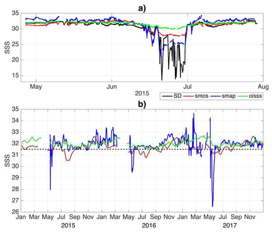
Figure 9.
(a), Time series of salinity measured by CTD on saildrone 128 (black) and collocated SSS from SMOS (red), SMAP (blue) and OISSS (green). (b), Time series for averaged SSS within a box near St. Matthew Island. The box location is marked in Figure 8b.
To evaluate the capabilities of satellite data in capturing the spring sea ice melting near St. Matthew Island, SSS time series within a boxed region near the island (Figure 8b) are constructed. Freshening events occur in May for year 2015 to 2017 in SMAP data (Figure 9b). The lowest SSS is well below the criterion of 31.5 isohaline. SSS in SMOS also drops below 31.5 PSS-78 in May, but its minimum is considerably larger than that in SMAP. In contrast, OISSS has high salinity (>31.5 PSS-78) over the entire period of 2015–2017. Interestingly, OISSS does show reduction in every May. It is speculated that the processing of OISSS eliminates the low SSS near sea ice edge but keeps the values near the boundary of fresh lens associated with sea ice melting.
3.2.2. Saildrone Missions in 2016
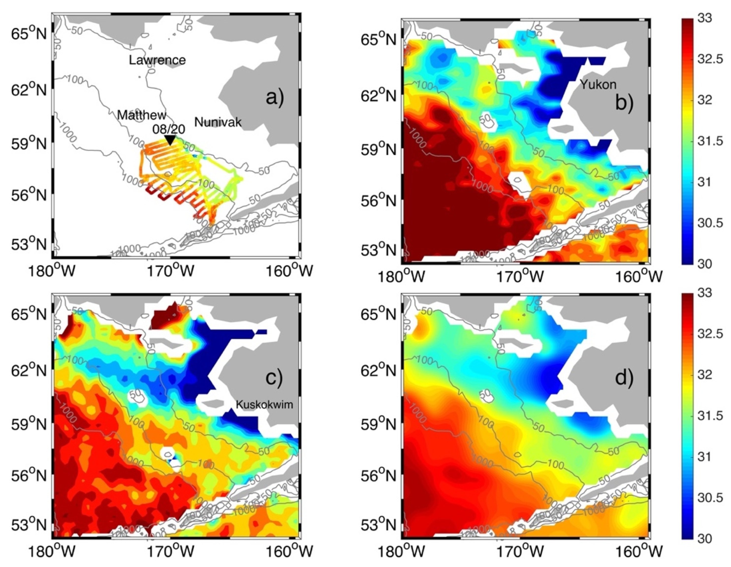
Saildrone vehicles SD126 and SD128 were deployed again on 23 May 2016 and recovered on 3 September. They stayed in the southern part of the shelf (south of 59° N). SD128 approached a mooring M2 (black triangle in Figure 10a) in early June. It recorded salinity values around 31.6 PSS-78. Satellite maps also exhibit relatively low SSS near the mooring during this period (Figure 10). Another striking feature captured by satellite data is a large area of coastal freshwater north of 59° N. Despite different values in SSS, all three satellite products reveal that a freshwater belt connects the Yukon River plume and the low SSS possibly induced by sea ice melting north of St. Matthew Island. This was formed under offshore winds. A similar event also took place in 2017, which will be discussed in the following section.
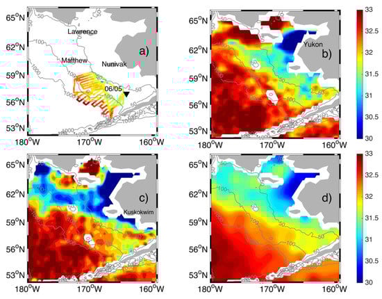
Figure 10.
(a) Salinity (color shading) from CTD on saildrone vehicles 126 and 128 along their trajectories. The launch site is the southern end of their tracks and time span is 23 May to 3 September 2016. Location (triangle) and passing time (month/day) for SD 128 are marked. The performance of three satellite products in early June is illustrated by snapshots extracted from SMOS (b), SMAP (c) and OISSS (d). Note, white area is missing data.
Saildrones spent the rest of June in the region south of 56°N and between the outer shelf (about 100 m water depth) and deep ocean (about 1000 m water depth) (Figure 11). Following their sawtooth pathway, the observed SSS displays larger values (about 32.5 PSS-78) over the deep ocean and fresher values (less than 32 PSS-78) in the shelf region. As shown in Figure 12a, the SSS fluctuations from mid-June to July largely reflect the spatial SSS gradient between deep ocean and shelf. They further navigated to north of 56° N in mid-July. Their survey was mostly confined between the 100-m and 50-m isobaths where SSS spatial difference is weaker. Consequently, the peak-to-peak range for SSS variability during this period is smaller than those in mid-June (Figure 12a).
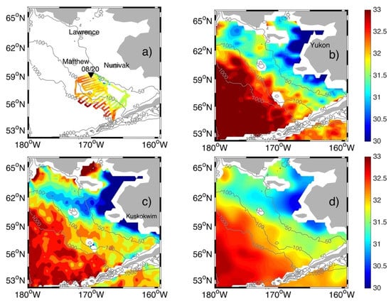
Figure 11.
Similar to Figure 10, but for the location of SD128 on 20 August 2016 (a), and SSS snapshots in middle August from SMOS (b), SMAP (c) and OISSS (d). Note, white area is missing data.
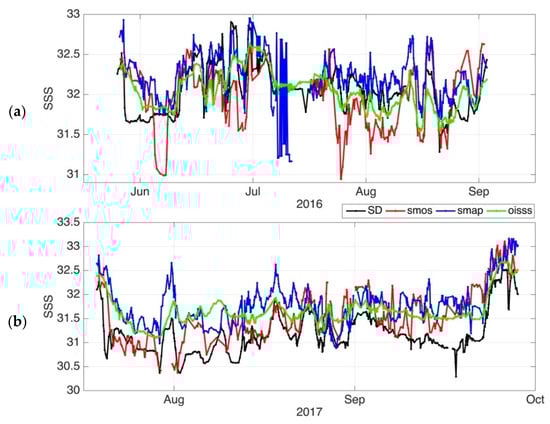
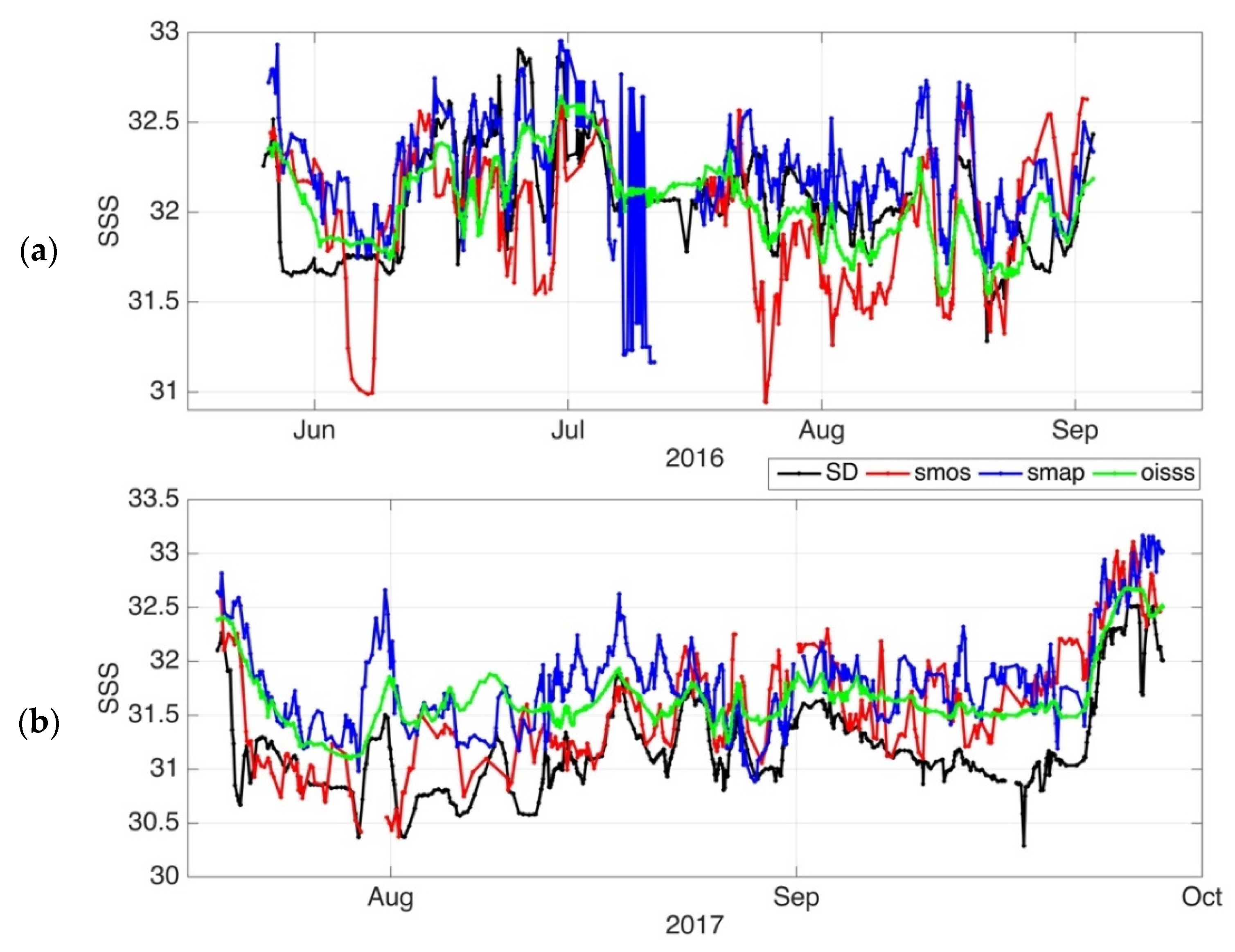
Figure 12.
Time series of salinity measured by CTD on saildrone (black) and collocated SSS from SMOS (red), SMAP (blue) and OISSS (green). Measurement from SD128 in 2016 and SD1001 in 2017 are displayed in (a,b), respectively.
Satellite maps in late August indicate that the freshwater discharge from the Kuskokwim River was intensified and advanced offshore. As a result, SSS in the middle shelf is lower than that in early June. Saildrone data also confirm the low SSS values near the 50 m isobath in late August (Figure 12a). This is in line with the SSS seasonal minimum in August-September for this region (Figure 7). SSS variations along the SD128 track are generally captured by satellite products.
Satellite products generally follows Saildrone records. However, SMOS and SMAP are much noisier than saildrone data (Figure 12a). OISSS tends to underestimate the high SSS peaks, but its performance is better than the other three satellite products based on the overall correlations with and mean biases against saildrone records (Table 1).
3.2.3. Saildrone Missions in 2017
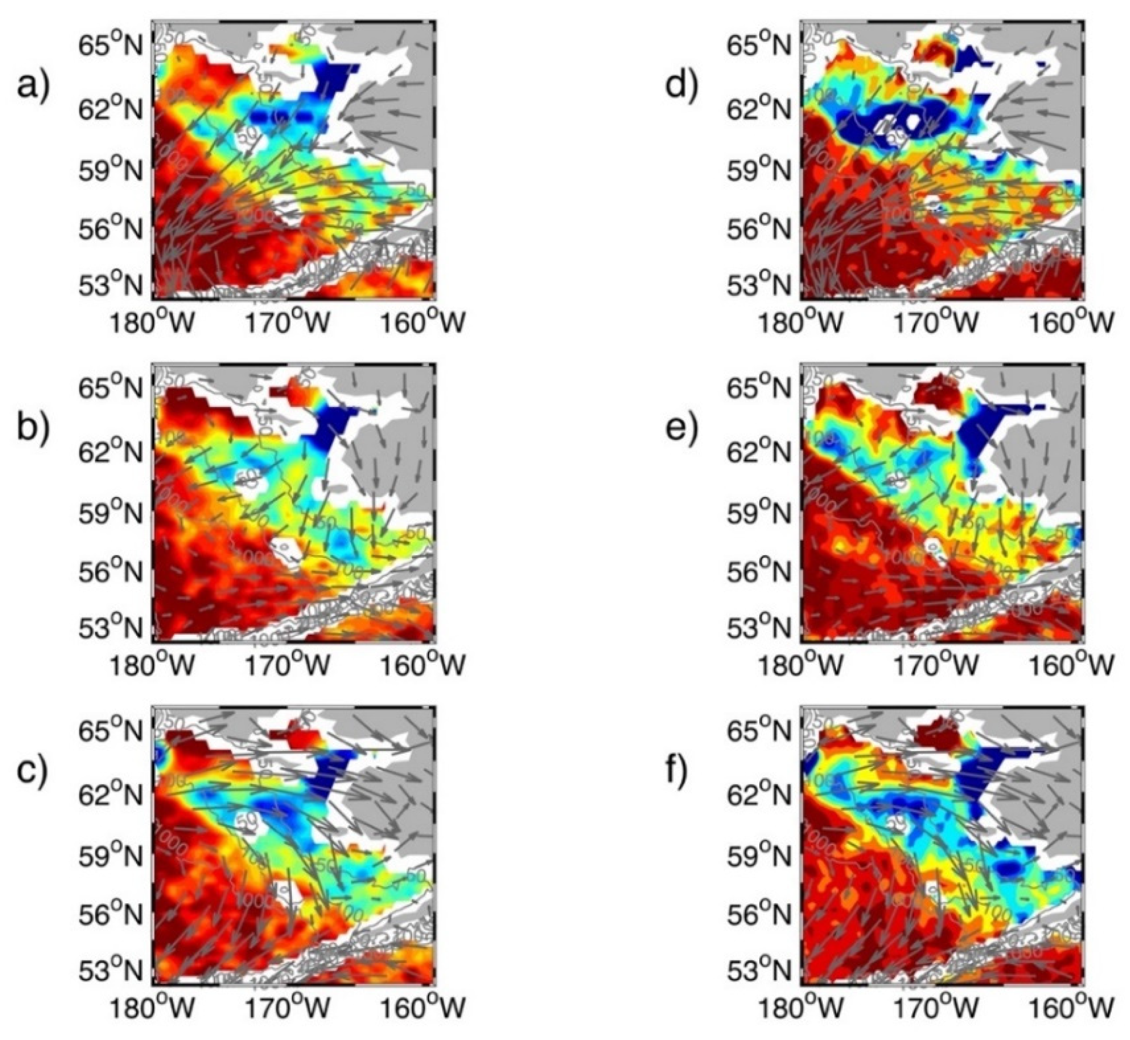
Three saildrone vehicles SD1001, SD1002, SD1003 were launched at Dutch Harbor, AK on 17 July 2017. Our analysis mostly focuses on the SD1001 data as both SD1002 and SD1003 navigated directly to the Arctic Ocean. Before their deployment, satellite maps capture the low SSS pattern on the northern shelf, which was induced by sea ice melting and river discharges (Figure 13a,d). The north-easterly wind provided favorable conditions (owing to Ekman transport) to push the river plume offshore, so that the plume was connected with the ice melting fresh water encircling St. Matthew Island. A similar freshwater belt was found in 2016 (Figure 10), indicating that it is not a rare event. The lens of low salinity is also mixed downward with subsurface higher salinity, which can account for the increased SSS in early June (Figure 13b,e). At the same time, the prevailing wind flipped to westerly and north-westerly and persisted until middle June. This promoted an offshore and southward ocean current to deliver more freshwater to the southern shelf (Figure 13c,f). South-easterly winds prevail from late June to middle July, during which the southward spread of low SSS is almost halted.
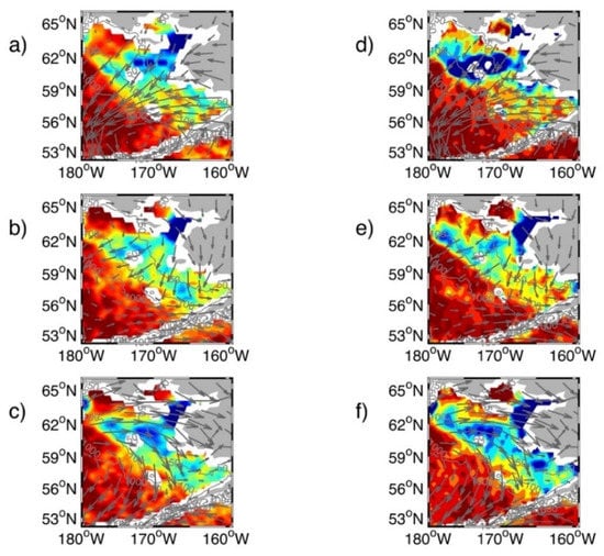
Figure 13.
Snapshots of SSS (color shading) from SMOS (left column) and SMAP (right column) in 15 May 2017 (a,d), 5 June 2017 (b,e) and 16 June 2017 (c,f). The color bar range is similar to Figure 11. The corresponding wind patterns are displayed in grey vectors. Note, white area is missing data.
From about 20 July, a few days after SD1001 was launched, surface wind force switched to westerly and north-westerly again. This then triggered the southward expansion of low salinity near the Yukon River and the Kuskokwim River. The SMOS map and SD1001 data both confirmed that the southern shelf was widely occupied by low SSS waters (Figure 14a,b). The wind became adverse for southward transport in August but supported the westward water movement north of St. Matthew Island (Figure 14c). Surface salinity in the southern shelf on 23 August was larger than in early August, likely resulting from horizontal and vertical mixing processes (Figure 14d).
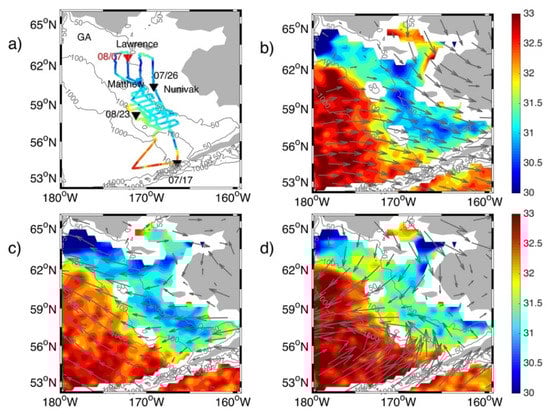
Figure 14.
(a) Salinity (color shading) from CTD on saildrone vehicles 1001. The launch site is the southern end of its track and time span is 17 July to 29 September 2017. Location (triangle) and passing time (month/day) for a few spots are marked. SSS snapshots from SMOS are shown on 26 July (b); 7 August (c); 23 August (d). The corresponding wind are in grey vectors. Note, white area is missing data.
SSS time series along the saildrone trajectories are consistent with the spatial patterns described above. It quickly reduced from 32.5 PSS-78 north of Dutch Harbor to 30.5–31 PSS-78 south of St. Lawrence (Figure 12b). When SD1001 surveyed between the 100-m and 50-m isobath in mid-August, the recorded SSS fluctuated between 32 PSS-78 and 31 PSS-78. Thus, SSS has a horizontal gradient of about 1 PSS-78 in this region. SSS increased to 32.5 PSS-78 after mid-September when the vehicle navigated to deeper water. All satellite products display rich fluctuations, but SMAP and OISSS apparently overestimate the surface salinity throughout the mission. In contrast, SMOS demonstrates overall agreement with saildrone data.
4. Discussion and Conclusions
The characteristics for SSS in the Bering Sea are extracted from an in situ observation-based dataset and three remote sensing satellite products. All of them capture the large-scale salinity front set up by salty water in the deep basin and freshwater along the coast of Alaska. The mean pattern of SSS is broadly consistent among different datasets, except for the substantial biases in SMAP off the coast of Siberia. Significant divergence between those products also exists on the eastern Bering Sea shelf. It should be stressed that CORA_OA might include dramatic uncertainties near the shallow waters and ice edge. Accordingly, discrepancies between satellite products and CORA_OA in those regions do not necessarily mean biases.
High SSS variability is found on the northern Bering Sea shelf, in particular in Norton Sound, the Gulf of Anadyr, and around St. Matthew Island. Such variability is pronounced in SMOS and SMAP but attenuated in OISSS. Not surprisingly, CORA_OA somewhat underestimates the standard deviation of SSS in those regions, indicating that its in situ measurements are insufficient in space and time to resolve the salinity variations. This also highlights the benefits of remote sensing data in understanding the salinity changes in the shelf region.
Thanks to lessened ice coverage in recent years, satellite data allows for the depiction of the SSS annual cycle over the entire Bering Sea. Both the deep ocean and eastern shelf are characterized by higher surface salinity in winter and lower values in summer months. The offshore expansion of coastal freshwater in summer and onshore retreat in winter are captured by all datasets. The peak-to-peak amplitude over a climatological annual cycle is only about 0.2–0.3 PSS-78 in the basin interior but exceeds 2 PSS-78 near the Gulf of Anadyr and St. Matthew Island. Its overall pattern resembles the structure of the standard deviations, suggesting that a large proportion of surface salinity changes take place on the seasonal time scale.
SSS normally reaches its seasonal maximum in winter and spring (from December to April) and minimum in summer (June-September). The timing or phase of the annual cycle is generally homogeneous in the deep ocean but displays patchy structures in the eastern Bering Sea shelf. Despite divergent behaviors in different datasets, consistency is found within each individual product. For instance, peak/trough times on the northern shelf (north of St. Matthew Island) and central shelf (50–100 m depths) are almost identical. This suggests that SSS fluctuates in phase across these regions. Previous analysis of hydrographic profiles pointed out that such coherence also applies to near-bottom salinity changes [17].
We also emphasize that remote sensing SSS in winter is valid in ice free or low-concentration areas. However, the early-stage sea ice formation is not monotonic, largely due to the variable surface wind fields. Periods of northerly or north-easterly winds result in ice advancing, while periods of southerly winds cause ice retreat. Multiple instances of ice advance and retreat were not uncommon in the eastern Bering Sea shelf [21]. The intermittent sea ice coverage and ice melting during those periods were widely documented [3,20,21,49]. Those short-term interruptions certainly modulate the specific SSS values and timing of the seasonal maximum. Even during stable and widely distributed sea ice extent periods, low salinity follows the ice edge where melting is frequent. However, the processing algorithms for different satellite products yield intrinsically varying skills in resolving the ice-ocean boundary. This is another source of uncertainty in the particular shape of the annual cycle over the southern part of the shelf.
SSS synoptic variability during the ice-free period is also dramatic over the shelf. The combination of saildrone measurements and satellite maps reveals the complexity of those SSS changes. Spring sea ice melting induces fresh layers encircling St. Matthew Island. Active vertical mixing prevents the persistence of that low SSS. Such rapid events of SSS reduction are successfully captured by SMAP, indicating that SMAP has promising applicability near the ice edge. On the other hand, the disappearance of sea ice also allows the low salinity water in Norton Sound and the Yukon River plume to be directly influenced by surface wind. As a frequently occurring wind pattern, northeasterlies drive freshwater westward and sometimes promote the formation of a long freshwater belt north of St. Matthew Island. According to satellite data, this phenomenon arose in both 2016 and 2017, suggesting that it is a typical process on the northern shelf. This also explains the enhanced SSS standard deviation in the vicinity of St. Matthew Island.
When the wind shifts to north-westerly, it provides a favorable condition for the spreading of the Yukon River plume to the southern shelf. Freshwater is visible on the central shelf, primarily in parallel with the 50 and 100-m isobaths. Another source of freshwater are the Kuskokwim River and other freshwater streams on the southwest coast of Alaska. Their signals are detectable in satellite maps in summer and early fall. When the southward transport of the Yukon River plume co-occurs with the discharge of Kuskokwim River or when one occurs after another, low SSS signals on the southern shelf can be sustained for longer time. It is true that SSS reaches its seasonal minimum from June to September, but the direction of the prevailing wind plays a critical role in controlling the detailed structure and timing of SSS minima over the shelf.
Both saildrone in situ observation and satellite maps provide unprecedented knowledge about the SSS variability in the seasonally ice-covered eastern Bering Sea shelf. Climate projections suggest that ice would retreat earlier and arrive later, which would allow for extended ice-free periods [50]. This further underscores the values of satellite data in monitoring winter and spring conditions in the future. In addition, a previous study has demonstrated that remote sensing salinity can reflect the SSS variability near major rivers in lower and middle latitudes [51]. Our assessment of satellite products near the Yukon River further confirms its robustness and benefits in understanding the intense salinity changes near such a high-latitude river. This has important implications in determining the most reliable dataset to study the salinity field in the Bering Sea and Arctic Ocean. While reanalysis products constructed from in situ measurements can serve as baseline for long-term mean features in these regions, remote sensing salinity is essential to understand both the time scale and spatial structure for their rapidly changing oceanic processes.
It should be admitted that uncertainties associated with satellite products are apparent, especially on the eastern Bering Sea shelf. The OISSS product is designed to correct satellite SSS biases using in situ SSS fields [52], but it missed much realistic variability near the coastal region and sea ice edge owing to a lack of in situ measurements there. During the three saildrone missions in 2015–2017, neither SMOS nor SMAP showed overwhelmingly better performance than the other. One particular issue is the resolvability near land and ice. The inconsistence between SMOS and SMAP near the Yukon River plume and ice-melting water around St. Matthew Island are very good examples. Their comparisons with individual Saildrone missions in 2015 demonstrate that SMOS tends to carry much larger positive biases than SMAP in these regions (Figure 9). Such overestimation in SMOS should be very common in other periods, as its long-term mean is higher near the Yukon River plume (Figure 1 and Figure 4). This problem also significantly affects its capability to record the SSS variability associated with sea ice melting. This is an important reason for the weaker standard deviations and lower peak-to-peak amplitude seasonal cycle in SMOS near St. Matthew Island (Figure 3 and Figure 5). Thus, more work should be carried out to further improve its performance near the land and ice.
Author Contributions
All the authors played a critical part in the preparation of the manuscript. Conceptualization, J.Z.; methodology, J.Z.; software, J.Z. and W.L.; validation, J.Z., Y.W., W.L. and H.B.; formal analysis, J.Z. and W.L.; investigation, J.Z., Y.W. and H.B..; resources, J.Z.; data curation, J.Z., E.D.C., C.W.M., N.L.-S., C.M.; writing—original draft preparation, J.Z.; writing—review and editing, Y.W., H.B., E.D.C.; visualization, J.Z.; supervision, J.Z.; project administration, J.Z.; funding acquisition, J.Z. All authors have read and agreed to the published version of the manuscript.
Funding
Y.W. is supported by Research Grants Council of Hong Kong (ECS26307720, GRF16305321). The Saildrone was developed through a public-private partnership between NOAA/PMEL and Saildrone Inc. Support for E.D.C., C.W.M., N.L.-S. and C.M. was through the Innovative Technology for Arctic Exploration (ITAE) program, a collaborative research effort between PMEL and the University of Washington (CICOES) that is funded by NOAA Research and PMEL.
Data Availability Statement
CORA dataset used in this research is publicly available (https://marine.copernicus.eu (accessed on 15 July 2021), the satellite salinity data is from https://podaac.jpl.nasa.gov (accessed on 16 July 2021). Saildrone data in 2015 and 2016 can be downloaded from https://www.ncei.noaa.gov/archive/archive-management-system/OAS/bin/prd/jquery/accession/details/187987 (accessed on 16 July 2021). Saildrone mission in 2017 is accessible at https://data.pmel.noaa.gov/pmel/erddap/index.html (accessed on 16 July 2021).
Acknowledgments
This is NOAA PMEL contribution number 5337, EcoFOCI contribution number 1021, and is a contribution to the Cooperative Institute for Climate, Ocean, & Ecosystem Studies (CIOCES) at the University of Washington under NOAA Cooperative Agreement NA20OAR4320271. Constructive comments from reviewers helped to improve the manuscript.
Conflicts of Interest
The authors declare no conflict of interest.
References
- Stabeno, P.J.; Schumacher, J.D.; Ohtani, K. The physical oceanography of the Bering Sea. In Dynamics of the Bering Sea: A Summary of Physical, Chemical, and Biological Characteristics, and a Synopsis of Research on the Bering Sea, North Pacific Marine Science Organization (PICES); Loughlin, T.R., Ohtani, K., Eds.; University of Alaska Sea Grant: Fairbanks, AK, USA, 1999; pp. 1–28. [Google Scholar]
- Hunt, G.L., Jr.; Stabeno, P.J.; Walters, G.; Sinclair, E.; Brodeur, R.D.; Napp, J.M.; Bond, N.A. Climate change and control of the southeastern Bering Sea pelagic ecosystem. Deep. Sea Res. II 2002, 49, 5821–5853. [Google Scholar] [CrossRef] [Green Version]
- Hunt, G.L., Jr.; Stabeno, P.J. Climate change and the control of energy flow in the southeastern Bering Sea. Prog. Oceanogr. 2002, 55, 5–22. [Google Scholar] [CrossRef] [Green Version]
- Aagaard, K.; Weingartner, T.J.; Danielson, S.L.; Woodgate, R.A.; Johnson, G.C.; Whitledge, T.E. Some controls on flow and salinity in Bering Strait. Geophys. Res. Lett. 2006, 33. [Google Scholar] [CrossRef]
- Danielson, S.L.; Weingartner, T.J.; Hedstrom, K.S.; Aagaard, K.; Woodgate, R.; Curchitser, E.; Stabeno, P.J. Coupled wind-forced controls of the Bering-Chukchi Shelf circulation and the Bering Strait throughflow: Ekman transport, continental shelf waves, and variations of the Pacific-Arctic sea surface height gradient. Prog. Oceanogr. 2014, 125, 40–61. [Google Scholar] [CrossRef] [Green Version]
- Woodgate, R.A.; Peralta-Ferriz, C. Warming and Freshening of the Pacific Inflow to the Arctic From 1990–2019 Implying Dramatic Shoaling in Pacific Winter Water Ventilation of the Arctic Water Column. Geophys Res Lett. 2021, 48, e2021GL092528. [Google Scholar] [CrossRef]
- Overland, J.E.; Salo, S.A.; Kantha, L.H.; Clayson, C.A. Thermal stratification and mixing on the Bering Sea shelf. In Dynamics of the Bering Sea: A summary of physical, chemical, and biological characteristics, and a synopsis of research on the Bering Sea; Loughlin, T.R., Ohtani, K., Eds.; University of Alaska Sea Grant: Fairbanks, AK, USA, 1999; pp. 129–146. [Google Scholar]
- Cokelet, E.D. 3-D water properties and geostrophic circulation on the eastern Bering Sea shelf. Deep Sea Res. Part II Top. Stud. Oceanogr. 2016, 134, 65–85. [Google Scholar] [CrossRef] [Green Version]
- Mysak, L.A.; Manak, D.K. Arctic sea-ice extent and anomalies, 1953–1984. Atmos. Ocean. 1989, 27, 376–405. [Google Scholar] [CrossRef]
- Francis, J.A.; Hunter, E. Drivers of declining sea ice in the Arctic winter: A tale of two seas. Geophys. Res. Lett. 2007, 34, 1–5. [Google Scholar] [CrossRef] [Green Version]
- Zhang, J.L.; Woodgate, R.; Moritz, R. Sea ice response to atmospheric and oceanic forcing in the Bering Sea. J. Phys. Oceanogr. 2010, 40, 1729–1747. [Google Scholar] [CrossRef]
- Stabeno, P.J.; Bell, S.W. Extreme Conditions in the Bering Sea (2017–2018): Record-Breaking Low Sea-Ice Extent. Geophys. Res. Lett. 2019, 46, 8952–8959. [Google Scholar] [CrossRef]
- Danielson, S.; Weingartner, T.; Aagaard, K.; Zhang, J.; Woodgate, R. Circulation on the central Bering Sea shelf, July 2008 to July 2010. J. Geophys. Res. 2012, 117, C10003. [Google Scholar] [CrossRef] [Green Version]
- Kachel, N.B.; Hunt, G.L., Jr.; Salo, S.A.; Schumacher, J.D.; Stabeno, P.J.; Whitledge, T.E. Characteristics and variability of the inner front of the southeastern Bering Sea. Deep Sea Res. Part II Top. Stud. Oceanogr. 2002, 49, 5889–5909. [Google Scholar] [CrossRef] [Green Version]
- Dean, K.G.; McRoy, C.P.; Ahlnas, K.; Springer, A. The plume of the Yukon River in relation to the oceanography of the Bering Sea. Remote Sens. Environ. 1989, 28, 75–84. [Google Scholar] [CrossRef]
- Cokelet, E.D.; Meinig, C.; Lawrence-Slavas, N.; Stabeno, P.J.; Mordy, C.W.; Tabisola, H.M.; Jenkins, R.; Cross, J.N. The use of Saildrones to examine spring conditions in the Bering Sea. In Proceedings of the OCEANS’15 MTS/IEEE Washington, Washington, DC, USA, 19–22 October 2015. [Google Scholar]
- Danielson, S.; Eisner, L.; Weingartner, T.; Aagaard, K. Thermal and haline variability over the central Bering Sea shelf: Seasonal and inter-annual perspectives. Cont. Shelf Res. 2011, 31, 539–554. [Google Scholar] [CrossRef]
- Chikita, K.A.; Wada, T.; Kudo, I.; Saitoh, S.-I.; Hirawake, T.; Toratani, M. Behaviors of the Yukon River Sediment Plume in the Bering Sea: Relations to Glacier-Melt Discharge and Sediment Load. Water 2021, 13, 2646. [Google Scholar] [CrossRef]
- Ladd, C.; Stabeno, P.J. Stratification on the Eastern Bering Sea shelf revisited. Deep Sea Res. II 2012, 65, 72–83. [Google Scholar] [CrossRef]
- Stabeno, P.J.; Schumacher, D.J.; Davis, F.R.; Napp, M.J. Under-ice observations of water column temperature, salinity and spring phytoplankton dynamics: Eastern Bering Sea shelf. J. Mar. Res. 1998, 56, 239–255. [Google Scholar] [CrossRef]
- Sullivan, M.; Kachel, N.B.; Mordy, C.W.; Salo, S.A.; Stabeno, P.J. Sea ice and water column structure on the eastern Bering Sea shelf. Deep Sea Res. Part II Top. Stud. Oceanogr. 2014, 109, 39–56. [Google Scholar] [CrossRef]
- Andreas, E.L.; Horst, T.; Grachev, A.; Persson, P.; Fairall, C.; Guest, P.; Jordan, R. Parametrizing turbulent exchange over summer sea ice and the marginal ice zone. Quart. J. Roy. Meteor. Soc. 2010, 136, 927–943. [Google Scholar] [CrossRef] [Green Version]
- Randelhoff, A.; Fer, I.; Sundfjord, A. Turbulent upper-ocean mixing affected by meltwater layers during Arctic summer. J. Phys. Oceanogr. 2017, 47, 835–853. [Google Scholar] [CrossRef] [Green Version]
- Vinogradova, N.; Lee, T.; Boutin, J.; Drushka, K.; Fournier, S.; Sabia, R.; Stammer, D.; Bayler, E.; Reul, N.; Gordon, A.; et al. Satellite salinity observing system: Recent discoveries and the way forward. Front. Mar. Sci. 2019, 6, 243. [Google Scholar] [CrossRef]
- Yu, L.; Bingham, F.M.; Lee, T.; Dinnat, E.P.; Fournier, S.; Melnichenko, O.; Tang, W.; Yueh, S.H. Revisiting the Global Patterns of Seasonal Cycle in Sea Surface Salinity. J. Geophys. Res. Ocean. 2021, 126, e2020JC016789. [Google Scholar] [CrossRef]
- Köhler, J.; Martins, M.S.; Serra, N.; Stammer, D. Quality assessment of spaceborne sea surface salinity observations over the northern North Atlantic. J. Geophys. Res. Oceans 2015, 120, 94–112. [Google Scholar] [CrossRef] [Green Version]
- Garcia-Eidell, C.; Comiso, J.C.; Dinnat, E.; Brucker, L. Satellite observed salinity distributions at high latitudes in the Northern Hemisphere: A comparison of four products. J. Geophys. Res. Ocean 2017, 122, 7717–7736. [Google Scholar] [CrossRef] [PubMed] [Green Version]
- Tang, W.; Yueh, S.; Yang, D.; Fore, A.; Hayashi, A.; Lee, T.; Fournier, S.; Holt, B. The potential and challenges of using SMAP SSS to monitor Arctic Ocean freshwater changes. Remote Sens. 2018, 10, 869. [Google Scholar] [CrossRef] [Green Version]
- UNESCO. The Practical Salinity Scale 1978 and the International Equation of State of Sea water 1980. UNESCO Tech. Pap. Mar. Sci. 1981, 25, 68. [Google Scholar]
- Olmedo, E.; Gabarró, C.; González-Gambau, V.; Martínez, J.; Ballabrera-Poy, J.; Turiel, A.; Portabella, M.; Fournier, S.; Lee, T. Seven years of SMOS sea surface salinity at high latitudes: Variability in Arctic and Sub-Arctic regions. Remote Sens. 2018, 10, 1772. [Google Scholar] [CrossRef] [Green Version]
- Reul, N.; Grodsky, S.A.; Arias, M.; Boutin, J.; Catany, R.; Chapron, B.; D’Amico, F.; Dinnat, E.; Donlon, C.; Fore, A.; et al. Sea surface salinity estimates from spaceborne L-band radiometers: An overview of the first decade of observation (2010–2019). Remote Sens. Environ. 2020, 242, 111769. [Google Scholar] [CrossRef]
- Fournier, S.; Lee, T.; Tang, W.; Steele, M.; Olmedo, E. Evaluation and Intercomparison of SMOS, Aquarius, and SMAP Sea Surface Salinity Products in the Arctic Ocean. Remote Sens. 2019, 11, 3043. [Google Scholar] [CrossRef] [Green Version]
- Fournier, S.; Lee, T.; Wang, X.; Armitage, T.W.K.; Wang, O.; Fukumori, I.; Kwok, R. Sea surface salinity as a proxy for Arctic Ocean freshwater changes. J. Geophys. Res. Ocean. 2020, 125, e2020JC016110. [Google Scholar] [CrossRef]
- Kubryakov, A.; Stanichny, S.; Zatsepin, A. River plume dynamics in the Kara Sea from altimetry-based lagrangian model, satellite salinity and chlorophyll data. Remote Sens. Environ. 2016, 176, 177–187. [Google Scholar] [CrossRef]
- Matsuoka, A.; Babin, M.; Devred, E.C. A new algorithm for discriminating water sources from space: A case study for the southern Beaufort Sea using MODIS ocean color and SMOS salinity data. Remote Sens. Environ. 2016, 184, 124–138. [Google Scholar] [CrossRef]
- Supply, A.; Boutin, J.; Vergely, J.-L.; Kolodziejczyk, N.; Reverdin, G.; Reul, N.; Tarasenko, A. New insights into SMOS sea surface salinity retrievals in the Arctic Ocean. Remote Sens. Environ. 2020, 249, 112027. [Google Scholar] [CrossRef]
- Chiodi, A.M.; Zhang, C.; Cokelet, E.D.; Yang, Q.; Mordy, C.W.; Gentemann, C.L.; Cross, J.N.; Lawrence-Slavas, N.; Meinig, C.; Steele, M.; et al. Exploring the Pacific Arctic Seasonal Ice Zone with Saildrone USVs. Front. Mar. Sci. 2021, 8, 640690. [Google Scholar] [CrossRef]
- Levine, R.M.; de Robertis, A.; Grünbaum, D.; Woodgate, R.; Mordy, C.W.; Mueter, F.; Cokelet, E.; Lawrence-Slavas, N.; Tabisola, H. Autonomous vehicle surveys indicate that flow reversals retain juvenile fishes in a highly advective high-latitude ecosystem. Limnol. Oceanogr. 2021, 66, 1139–1154. [Google Scholar] [CrossRef]
- Vazquez-Cuervo, J.; Gentemann, C.; Tang, W.; Carroll, D.; Zhang, H.; Menemenlis, D.; Gomez-Valdes, J.; Bouali, M.; Steele, M. Using Saildrones to Validate Arctic Sea-Surface Salinity from the SMAP Satellite and from Ocean Models. Remote Sens. 2021, 13, 831. [Google Scholar] [CrossRef]
- Meinig, C.; Lawrence-Slavas, N.; Jenkins, R.; Tabisola, H.M. The use of Saildrones to examine spring conditions in the Bering Sea: Vehicle specification and mission performance. In Proceedings of the OCEANS 2015-MTS/IEEE Washington, Washington, DC, USA, 19–22 October 2015. [Google Scholar]
- Mordy, C.W.; Cokelet, E.D.; De Robertis, A.; Jenkins, R.; Kuhn, C.E.; Lawrence-Slavas, N.; Berchok, C.L.; Crance, J.L.; Sterling, J.T.; Cross, J.N.; et al. Advances in Ecosystem Research Saildrone Surveys of Oceanography, Fish, and Marine Mammals in the Bering Sea. Oceanography 2017, 30, 113–115. [Google Scholar] [CrossRef]
- Cabanes, C.; Grouazel, A.; von Schuckmann, K.; Hamon, M.; Turpin, V.; Coatanoan, C.; Paris, F.; Guinehut, S.; Boone, C.; Ferry, N.; et al. The CORA dataset: Validation and diagnostics of in-situ ocean temperature and salinity measurements. Ocean. Sci. 2013, 9, 1–18. [Google Scholar] [CrossRef] [Green Version]
- Szekely, T.; Gourrion, J.; Pouliquen, S.; Reverdin, G. The CORA 5.2 dataset for global in situ temperature and salinity measurements: Data description and validation. Ocean Sci. 2019, 15, 1601–1614. [Google Scholar] [CrossRef] [Green Version]
- Meissner, T.; Wentz, F.; Le Vine, D. The salinity retrieval algorithms for the NASA Aquarius version 5 and SMAP version 3 releases. Remote Sens. 2018, 10, 1121. [Google Scholar] [CrossRef] [Green Version]
- Boutin, J.; Vergely, J.L.; Khvorostyanov, D. SMOS SSS L3 Maps Generated by CATDS CEC LOCEAN Debias V5.0. Available online: https://www.seanoe.org/data/00417/52804/ (accessed on 8 September 2021).
- Melnichenko, O. Multi-Mission L4 Optimally Interpoated Sea Surface Salinity. Ver. 1.0. PO.DAAC, CA, USA. Available online: https://doi.org/10.5067/SMP10-4U7CS (accessed on 30 September 2021).
- Mesinger, F.; DiMego, G.; Kalnay, E.; Mitchell, K.; Shafran, P.C.; Ebisuzaki, W.; Jović, D.; Woollen, J.; Rogers, E.; Berbery, E.H.; et al. North American Regional Reanalysis. Bull. Am. Meteorol. Soc. 2006, 87, 343–360. [Google Scholar] [CrossRef] [Green Version]
- Danielson, S.; Hedstrom, K.; Aagaard, K.; Weingartner, T.; Curchitser, E. Wind-induced reorganization of the Bering shelf circulation. Geophys. Res. Lett. 2012, 39, L08601. [Google Scholar] [CrossRef]
- Alexander, V.; Niebauer, H.J. Oceanography of the eastern Bering Sea ice-edge zone in spring. Limnol. Oceanogr. 1981, 26, 1111–1125. [Google Scholar] [CrossRef]
- Wang, M.; Yang, Q.; Overland, J.E.; Stabeno, P.J. Sea-ice cover timing in the Pacific Arctic: The present and projections to mid-century by selected CMIP5 models. Deep. Sea Res. Part II Top. Stud. Oceanogr. 2018, 152, 22–34. [Google Scholar] [CrossRef] [Green Version]
- Fournier, S.; Lee, T. Seasonal and Interannual Variability of Sea Surface Salinity Near Major River Mouths of the World Ocean Inferred from Gridded Satellite and In-Situ Salinity Products. Remote Sens. 2021, 13, 728. [Google Scholar] [CrossRef]
- Melnichenko, O.; Hacker, P.; Maximenko, N.; Lagerloef, G.; Potemra, J. Optimal interpolation of Aquarius sea surface salinity. J. Geophys. Res. Oceans 2016, 121, 602–616. [Google Scholar] [CrossRef] [Green Version]


Publisher’s Note: MDPI stays neutral with regard to jurisdictional claims in published maps and institutional affiliations. |
© 2022 by the authors. Licensee MDPI, Basel, Switzerland. This article is an open access article distributed under the terms and conditions of the Creative Commons Attribution (CC BY) license (https://creativecommons.org/licenses/by/4.0/).