Communication

Remote Sensing Monitoring of Winter Wheat Stripe Rust Based on mRMR-XGBoost Algorithm

1
College of Geometrics, Xi’an University of Science and Technology, Xi’an 710054, China
2
Key Laboratory of Digital Earth Science, Aerospace Information Research Institute, Chinese Academy of Sciences, Beijing 100094, China
*
Author to whom correspondence should be addressed.
Remote Sens. 2022, 14(3), 756; https://doi.org/10.3390/rs14030756
Submission received: 15 December 2021 / Revised: 26 January 2022 / Accepted: 3 February 2022 / Published: 6 February 2022
(This article belongs to the Special Issue Recent Progress in UAV-AI Remote Sensing)

Abstract

:
For the problem of multi-dimensional feature redundancy in remote sensing detection of wheat stripe rust using reflectance spectrum and solar-induced chlorophyll fluorescence (SIF), a feature selection and disease index (DI) monitoring model combining mRMR and XGBoost algorithm was proposed in this study. Firstly, characteristic wavelengths selected by successive projections algorithm (SPA) were combined with the vegetation indices, trilateral parameters, and canopy SIF parameters to constitute the initial feature set. Then, the max-relevance and min-redundancy (mRMR) algorithm and correlation coefficient (CC) analysis were used to reduce the dimensionality of the initial feature set, respectively. Features selected by mRMR and CC were input as independent variables into the extreme gradient boosting regression (XGBoost) and gradient boosting regression tree (GBRT) to monitor the severity of stripe rust. The experimental results show that, compared with CC analysis, the monitoring accuracy of the features selected by mRMR in the XGBoost and GBRT models increased by 12% and 17% on average, respectively. Meanwhile, the mRMR-XGBoost model achieved the best monitoring accuracy (R2 = 0.8894, RMSE = 0.1135). The R2 between the measured DI and predicted DI of mRMR-XGBoost was improved by an average of 5%, 12%, and 22% compared with mRMR-GBRT, CC-XGBoost, and CC-GBRT models. These results suggested that XGBoost is more suitable for the remote sensing monitoring of wheat stripe rust, and mRMR has more advantages than the commonly used CC analysis in feature selection. Field survey data validation results also confirm that the mRMR-XGBoost algorithm has excellent monitoring applicability and scalability. The proposed model could provide a reference for data dimensionality reduction and crop disease index monitoring based on hyperspectral data.

1. Introduction

Wheat stripe rust is a pandemic disease caused by Puccinia striiformis f. sp. tritici that can achieve cross-regional initial and re-infection through airflow. It is one of the most important disease types for wheat prevention and control in China [1]. Due to the lack of precise remote sensing monitoring technology for crop diseases, the production is generally based on undifferentiated regional control. This increases the cost of wheat planting and pesticide residues in the cultivated land. With the advancement of agricultural informatization, hyperspectral data is widely used in remote sensing monitoring of crop diseases. However, the high-dimensional and small sample data characteristics of hyperspectral data make their direct application ineffective. Extracting disease-sensitive features in hyperspectral data is the most potential method to solve feature redundancy.
In the VIS-NIR spectrum, various symptoms and physiological changes of diseases show specific responses in spectral reflectance [2]. The identification of crop diseases and prediction of disease severity can be realized by using the sensitive wavelengths of spectral response and the variation of the abnormal spectrum. On this basis, the spectral vegetation index constructed by sensitive spectrum combinations in hyperspectral data shows a clear relation to the physiological and biochemical processes of crops that are infected by pathogens. Several researches have shown that the spectral vegetation indices have additionally the potential to detect and differentiate plant diseases [3,4]. Meanwhile, specific form changes of the original hyperspectral data can enhance the difference in spectral characteristics [5]. These methods mainly extract and construct relevant spectral features by searching for hyperspectral bands that are more sensitive to disease severity. But a quantitative statement or the identification of a specific disease is impossible so far since these methods lack disease specificity. Therefore, choosing a suitable model construction method is the key to realizing the crop diseases remote sensing monitoring research in recent years [6,7]. The combination of hyperspectral feature selection and machine learning model has been applied to the research of some crop diseases identification and detection [8]. However, these researches are mostly based on reflectance spectrum data, which is greatly affected by background noise. Moreover, the reflectance spectrum mainly reflects the concentration information of biochemical components, which cannot directly reveal the photosynthetic physiological state of vegetation [9]. Solar-induced chlorophyll fluorescence (SIF) can non-destructively detect the photosynthetic physiology and stress status of plants [10]. More importantly, the SIF signal comes entirely from the measured crop, which is purer than the reflectance data. Comprehensive utilization of the advantages of reflectance spectroscopy in the detection of crop biochemical parameters and the advantages of SIF in the diagnosis of photosynthetic physiology, which can objectively reflect the real condition of crops under disease stress and improve the accuracy of remote sensing detection [11]. Jing et al. used the GA-SVR model to optimize the initial feature set and model parameters composed of reflectance features and SIF parameters, which achieved high-precision prediction of the severity of stripe rust [12]. However, as a random search method, genetic algorithm takes a long time to get a more accurate solution, and its efficiency still needs improvement. Compared with the current popular machine learning models, the extreme gradient boosting regression (XGBoost) has the appealing properties of limited sample learning, fast model training, strong mathematical explanation ability, and data feature invariance [13].
These researches only pay attention to the influence of the selected feature parameters as the input factors of the machine learning model on the prediction accuracy of crop disease severity and ignore the redundancy between the selected feature parameters. According to the above statement, the initial feature set of this study consisted of the selected reflectance indices and canopy SIF parameters. Then, the feature combination was selected from the initial set by the max-relevance and min-redundancy (mRMR) algorithm, which had the maximal relevance with the stripe rust disease index and the minimal redundancy among the selected features. These features were input as independent variables into the XGBoost model to construct a remote sensing monitoring model for the severity of wheat stripe rust disease.

2. Materials and Methods

2.1. Field Experimental Data Acquirement

The experiment was conducted at China Agricultural Science Experimental Station, Langfang City, Hebei Province (39°30′40″N, 116°36′20″E). The wheat cultivar in the study area is Mingxian 169, which is more sensitive to stripe rust. On 9 April 2018 (wheat rising period), a spore solution with a concentration of 0.09 mg/mL was used to inoculate wheat stripe rust by spraying. The study area was divided into healthy groups and infected groups. A 5-m isolation zone was set up between the healthy groups and the infected groups, and the healthy groups were sprayed with pesticides. Canopy spectrum data of wheat stripe rust in different severity were measured on May 18 (226 d after sowing), May 24 (232 d after sowing), and May 30 (232 d after sowing) by ASD Field Spec 4 surface spectrometer. Measurements were carried out between 11:00 and 12:30 Beijing time to reduce the influence of observation angle and solar zenith angle. In addition, the canopy radiance data were corrected by the standard BsSO4 board before data collection. The disease index (DI) of wheat stripe rust was investigated using a 5-point sampling method [14]. On each inspection, the plants were grouped into one of nine classifications of disease incidence (0, 1%, 10%, 20%, 30%, 45%, 60%, 80%, and 100%). According to Equation (1), DI can be calculated based on the number of wheat leaves recorded at each severity level.
DI = ( m × f ) n × f
where, DI is the disease index, m is the value of each gradient, n is the highest gradient level value, and the f is the number of leaves in each gradient.

2.2. Extraction of Canopy SIF Parameters

Solar-induced chlorophyll fluorescence (SIF) has a filling effect at the Fraunhofer dark line. Based on this, scholars have proposed single-band SIF extraction methods such as FLD, 3FLD, and iFLD [15,16]. Existing studies have shown that 3FLD is more robust, which provides a more accurate estimation of SIF signal under different signal-to-noise ratios conditions [17]. Therefore, the 3FLD method was chosen to extract the canopy SIF radiation in the O2-A and O2-B bands, which can be estimated according to Equation (2). Moreover, to eliminate the influence of external factors at different time periods on canopy SIF, this study adopted relative SIF as the canopy SIF [18]. Its calculation is shown in Equation (3).
F   ¯ in = ( ω left I left + ω right I right ) L in I in ( ω left L left + ω right L right ) ( ω left I left + ω right I right ) I in
F relative = F   ¯ in / I in
where F   ¯ in is the canopy SIF radiation. ωleft and ωright represent the weight of the left and right bands. Lin, Lleft, and Lright represent the canopy reflectance radiance inside, left, and right of the absorption band. Iin, Ileft, and Iright represent the solar irradiance inside, left, and right of the absorption band. In addition to calculating the canopy SIF directly by radiance, the reflectance band at 650–800 nm, which is greatly affected by chlorophyll fluorescence, can be used to obtain a reflectance index that can reflect the intensity of fluorescence as well. Therefore, this study also elects the reflectance ratio index [19] and the reflectance first derivative index [20] as the fluorescence feature input of the model. The definitions of selected canopy SIF parameters are listed in Table 1.

2.3. Calculation of Hyperspectral Vegetation Indices

Varieties in physiological, biochemical characteristics and apparent morphology of crops under disease stress cause changes in spectral characteristics. Its spectral response could be seen as a function of changes in pigments, water, morphology, and structure [21]. Spectral index constructed by the sensitive bands can reflect the change of spectral response, so as to realize the monitoring of the disease from the perspective of the pathological mechanism. According to the above statement, this paper selects vegetation indices related to pigments such as GI, PRI, SIPI, PSRI, and MCARI [22,23,24,25,26], and water-related indices WI and NDWI [27,28], as well as the TVI and RTVI that characterizes the morphology and structure of the plant canopy and the HI that indicates whether the vegetation is healthy or not [3,29,30]. Differential spectrum has an advantage in eliminating or reducing the influence of background and noise spectrum. When the canopy coverage reaches more than 20%, the soil background has little effect on the first-order differential [31]. Combined with the existing research on wheat stripe rust monitoring with hyperspectral trilateral parameters [32], this study also selects Db, SDb, Dy, SDy, Dr, and SDr. And their definitions are listed in Table 2.

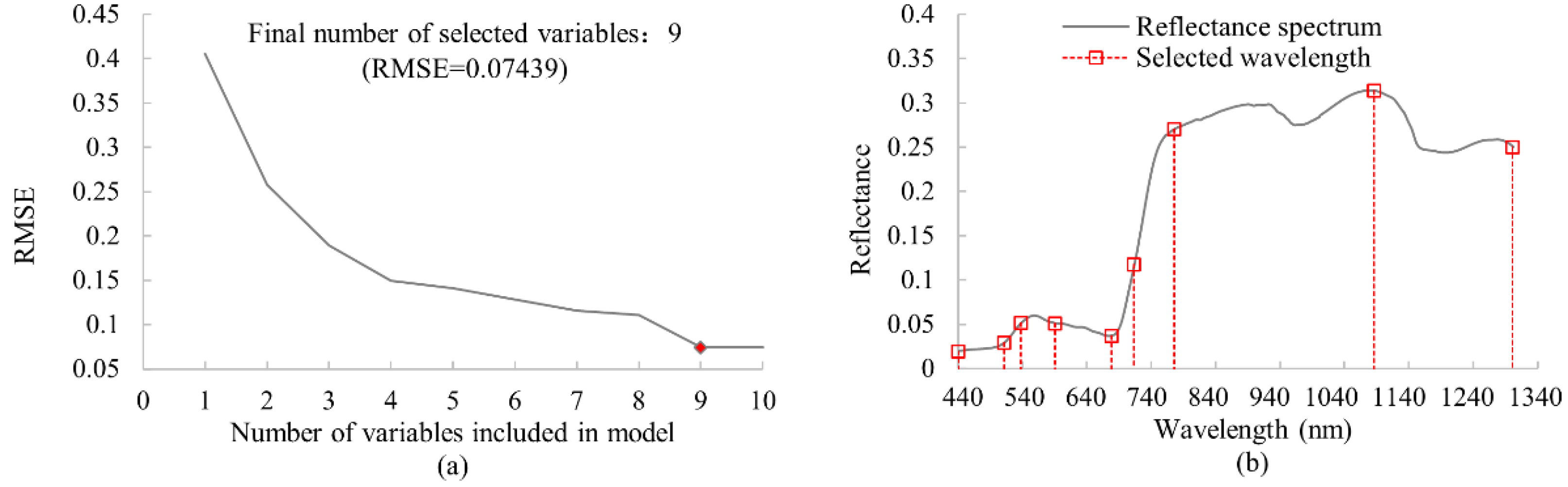
2.4. Extraction of Characteristic Band
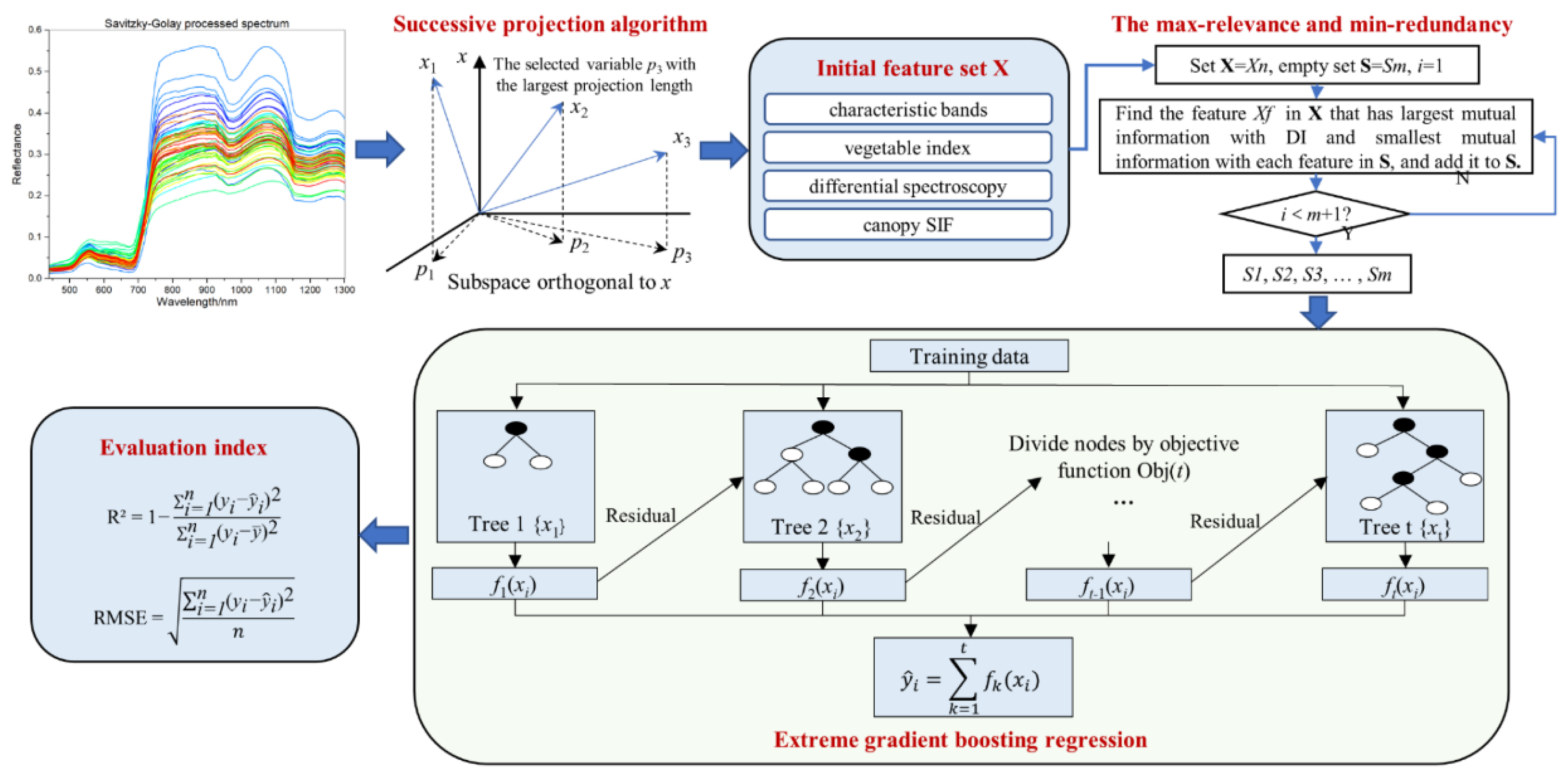
As a deterministic search methodology, successive projections algorithm (SPA) has reproducible results. It is more reliable in the selection of the verification set. It can find the variable group with the lowest redundant information from the spectral information, while retaining most of the features of the original spectrum [33]. The selected waveband has a clear physical meaning, which can better explain the response of the spectral shape and intensity changes to crop diseases. Based on SPA, the characteristic bands were selected from the hyperspectral data after Savitzky-Golay smoothing. The pros and cons of the algorithm are measured by the root mean square error (RMSE). According to the internal cross-validation RMSE of the training set, nine characteristic bands (RMSE = 0.074) are obtained, and the selected wavelength positions are shown in Figure 1. Since SPA is greatly affected by the first band, this study only selects the first six important bands as the model feature input (R539, R513, R1086, R776, R713, R678). These wavelengths are located in the absorption peaks (R776, R1086), absorption valleys (R678, R513), and relatively large slopes (R539, R713) of the spectral curve, which are typical disease response intervals and can sensitively reflect stripe rust stress.

2.5. Methods

2.5.1. The Max-Relevance and Min-Redundancy Feature Selection

With mRMR, which is one of the feature selection methods, a subset is created in which the related properties of the data are retrieved and the unrelated features are discarded [34]. To measure the similarity among elements in the initial set X, the algorithm accepts each feature as a discrete variable and uses the mutual information. Suppose the probability density and joint probability density of feature a and b are p(a), p(b), and p(a, b), respectively. The calculation formula of mutual information F between two features can be defined as Equation (4).
F ( x , y ) = a b p ( a , b ) log ( p ( a , b ) p ( a ) p ( b ) ) d a d b
Then, the mutual information between each feature and DI is calculated in turn according to Equation (5), and the feature with the maximum value is input into the subset S. In this way, a subset S with j features Xf can be found from the initial feature set X. That is, the features in the subset all have high relevance with DI.
m a x R 1 ( S , D I ) ,   R 1 = 1 | S | X f F ( X f , D I )
Theoretically, the relevance between the first j features and the DI value is maximal. But the correlation between these features may also be large, which means that the redundancy is high. Therefore, the principle of least redundancy can be used to filter out redundant features.
m i n R 2 ( S ) , R 2 = 1 | S | 2 X f , X l S F ( X f , X l )
where Xf and Xl are features in subset S. The combination of Equations (5) and (6) is the mutual information quotient (MIQ) criteria, the selected features have maximal relevance with the disease index and minimal redundancy with each other.
MIQ = m a x X f Ω S [ F ( X f , DI ) / 1 | S | X f , X l S F ( X f , X l ) ]

2.5.2. Extreme Gradient Boosting Regression

In this study, features selected by the mRMR algorithm were inputted as independent variables into XGBoost regression to construct a remote sensing monitoring model for stripe rust. XGBoost integrates weak classifiers into strong classifiers and iteratively generates new trees to fit the residuals of the previous trees [35]. As the number of iterations increases, the accuracy continues to improve. For a given training set consisting of n samples and m feature groups, D = (xi, yi), where | D | = n , x i R m , y i R . The mathematical model of the XGBoost algorithm can be regarded as an additive model composed of t regression trees. The predicted value of the model can be calculated by the following formula.
y ^ i = k = 1 t f k ( x i )
where t is the number of trees, y i and y ^ i are measured and predicted values, respectively, fk is the function represented by the kth independent tree, and fk(xi) is the space of the CART regression tree. The objective function of the XGBoost algorithm can be constructed as the Equation (9).
O b j ( k ) = i = 1 n l [ ( y i , y ^ ( k 1 ) ) + f k ( x i ) ] + Ω ( f k ) + c o n s
Ω ( f k ) = γ T k + 1 2 λ || ω k || 2
where Ω ( f k ) is the regularization term, that is, the sum of the complexity of each tree. It can control the complexity of the model and prevent overfitting. γ and λ are the model’s penalty coefficient and L2 regular term coefficient, T is the number of leaf nodes, and ω represents the leaf score. Compared with the traditional gradient boosting trees, the XGBoost regression incorporates initial derivative information into the optimization process, performs secondary Taylor expansion of the loss function, and adjusts the complexity of model fitting to prevent overfitting together with loss function regularization.
O b j ( k ) i = 1 n l [ ( y i , y ^ ( k 1 ) ) + g i f k ( x i ) + 1 2 h i f k 2 ( x i ) ] + Ω ( f k )
where g i = ( l ( y i , y ^ ( k 1 ) ) ) y ^ ( k 1 ) , h i = 2 ( l ( y i , y ^ ( k 1 ) ) ) y ^ ( k 1 ) , which are the first derivative and second derivative of the loss function to the current model, respectively. Therefore, the objective function can be expressed as Equation (12).
O b j ( k ) = j = 1 T [ j I j g j ω j + 1 2 ( j I j h j + λ ) ω j 2 ] + γ T
where Ij represents the set of samples on the leaf node whose sequence number is j. Find the optimal solution to equation (8) and bring it back to the equation to obtain the minimized objective function of the XGBoost model.
O b j ( k ) = 1 2 j = 1 T ( j I j g j ) 2 j I j h j + λ + + γ T
The smaller Obj(k), the better the structure of the tree. During the training process, the XGBoost algorithm corrects the previous tree model through iterative residuals to optimize the specified loss function. XGBoost with the CART booster has more than 20 parameters, but the number of estimators, learning rate, minimum child weight, maximum tree depth, subsample ratio of training samples and alpha are the most important parameters. In this research, the optimal values of the above six parameters were obtained through the grid parameter optimization method. After obtaining the model parameters that best fit the train data, combining the mRMR algorithm and XGBoost regression could quickly achieve an accurate predictive disease index value with as few features as possible. The process framework of this research method is shown in the Figure 2.

3. Results and Analysis

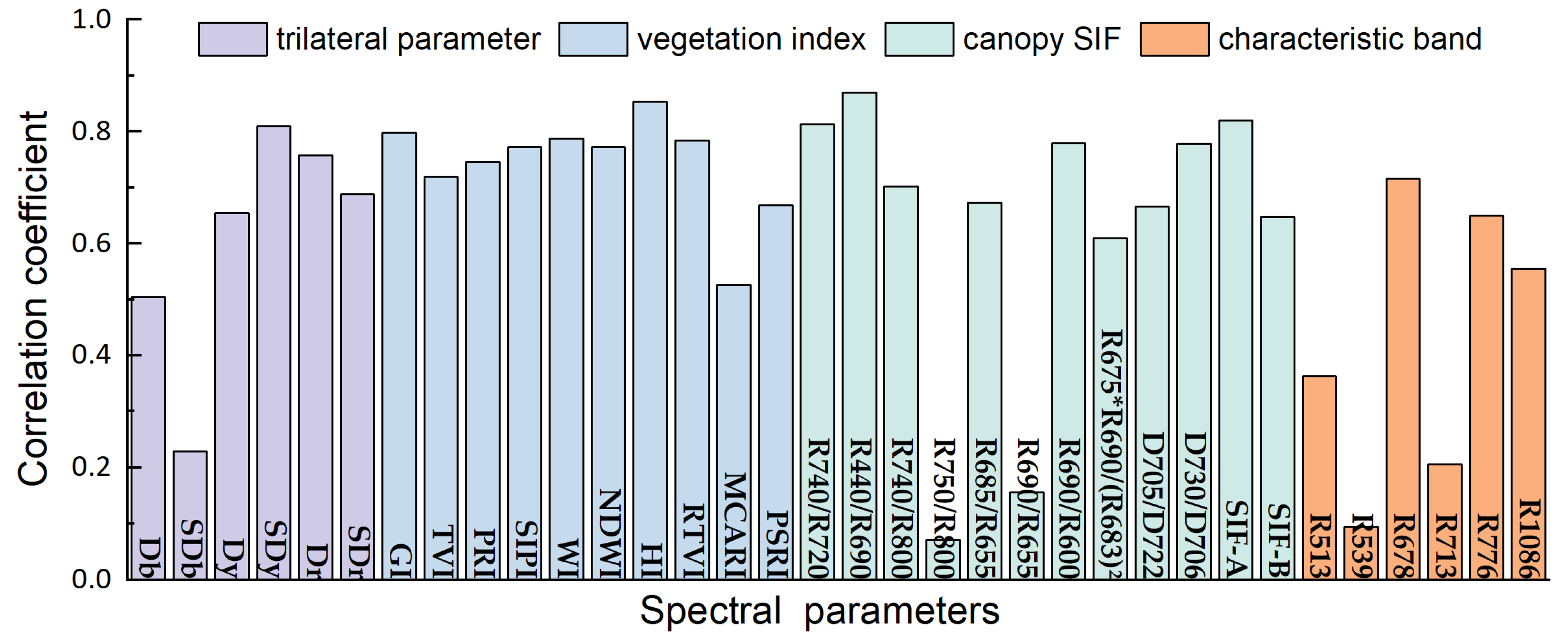
3.1. Features Selected by CC

The initial feature set is composed of 12 canopy SIF parameters, 10 vegetation indices, 6 trilateral parameters, and 6 characteristic bands. Parameters in the feature set are analysed with DI one by one, the correlation coefficient between each feature parameter and DI is shown in Figure 3. It can be seen from Figure 3 that the overall selected vegetation indices have high correlations with the DI. The winter wheat which has been affected by stripe rust has obvious responses in terms of pigment, water content, and canopy structure. In addition, canopy chlorophyll fluorescence parameters are sensitive to stripe rust stress. In the trilateral parameters, the area and amplitude of the red and yellow edges are more obvious in response to wheat stripe rust. Since SPA selects the wavelength combination with the least collinearity, and the combination contains the majority information of total spectral reflectance. Therefore, the correlation coefficient between each wavelength and the DI shows non-uniformity. According to Figure 3, this study selected 6 parameters that are extremely significantly related to DI (p < 0.01), including SIF-A, R440/R690, R740/R720, HI, GI and SDy.

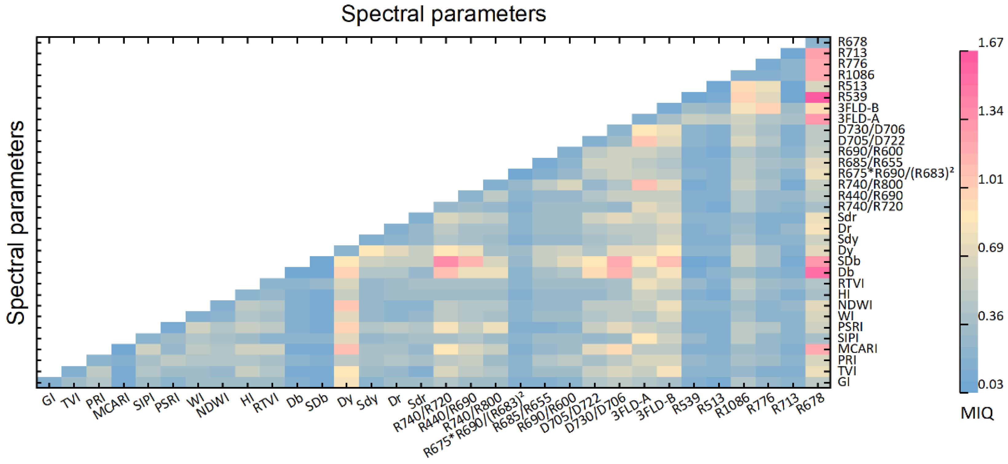
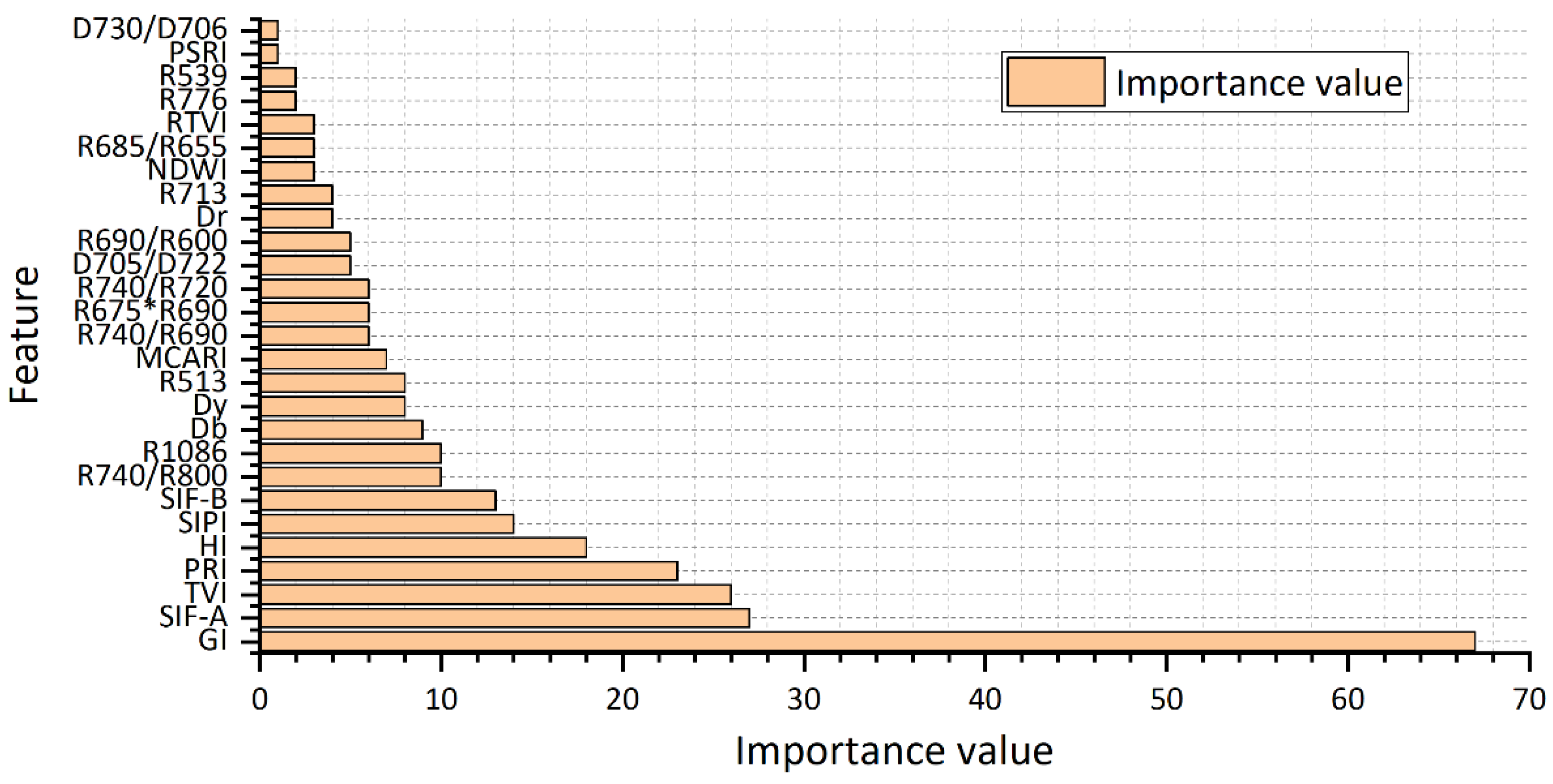
3.2. Features Selected by mRMR

The mRMR feature selection algorithm is used to filter the initial feature set, so that related features are concentrated, and irrelevant features are minimized. The MIQ of each spectral parameter and DI is shown in Figure 4. The warmer the grid color, the higher the MIQ, that is, the feature in the grid has a high correlation with DI and low redundancy with other features. It can be seen from Figure 4, there are eight parameters (Dy, R740/R720, R440/R690, D705/D722, D730/D706, SIF-A, SIF-B, R1086, and R678) with higher MIQ values. Corresponding to the CC analysis, six features were selected according to grid color as input parameters for the remote sensing monitoring of the wheat stripe rust severity (R740/R720, SIF-A, Dy, R678, R1086, and R440/R690), including three SIF parameters, two characteristic bands, and one trilateral spectral index. Selected features had the maximum MIQ with each other compared to the others. In addition, although those vegetation indices had an obvious correlation with DI, their MIQ values were extremely low as seen in Figure 4. It was proved that vegetation indices have high redundancy among each other. Thus, mRMR feature selection did not choose any vegetation index.

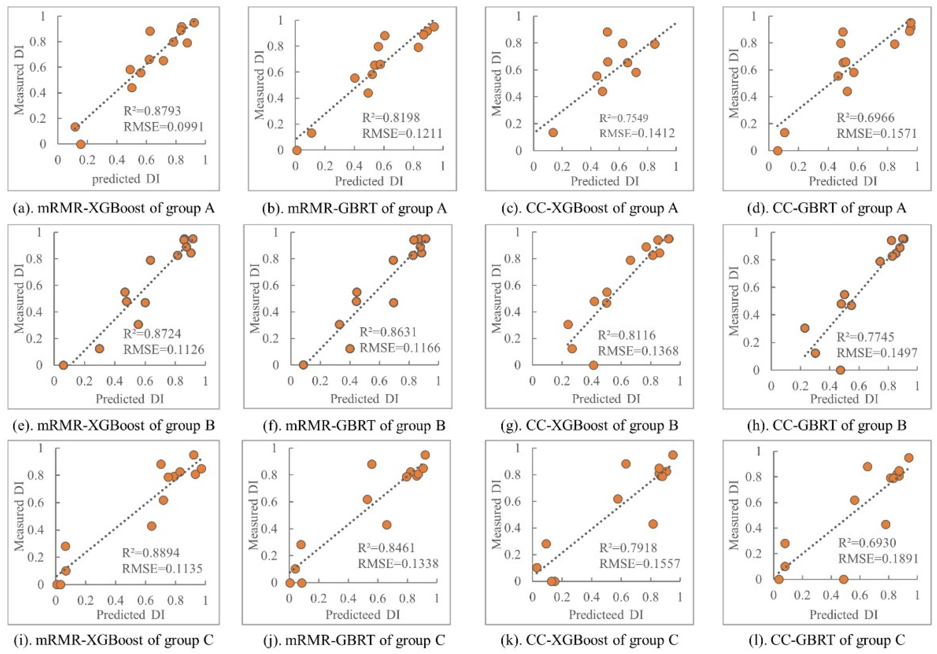
3.3. Remote Sensing Monitoring Model of Wheat Stripe Rust

In order to ensure the stability and reliability of the evaluation results, improve the generalization ability of the model, and reduce the impact of a random grouping of sample data on the accuracy of the model. In this study, 52 samples (47 infected samples, 5 healthy samples) were grouped repeatedly for three times (A, B, C). Each group is randomly divided into training set and validation set according to a ratio of 3:1, including 39 samples in the training set and 13 samples in the validation set. The determination coefficient (R2) and Root Mean Square Error (RMSE) between the predicted value and the measured value are selected as the model accuracy evaluation indicators.
Based on the given step size and optimization accuracy range, the parameters of the training set were continuously iteratively adjusted through grid parameter optimization. Figure 5 illustrates the RMSE values versus the combination of these four parameters based on train data. Since the n_estimators and learning_rate have the greatest impact on the model, these two parameters were optimized first. It is worth noting that when these two parameters were configured, the remaining parameters took the default values. On the basis of the optimal learning_rate and n_estimators, the subsample and reg_alpha were optimized. Repeat this process until the optimal values of the six parameters were found.
According to Figure 5, grid parameter optimization selects the two parameters corresponding to the grid at the minimum RMSE. It can be seen from Figure 5a that the learning rate has a stable RMSE value between 0.2 and 0.4. Beyond this interval, the algorithm becomes more conservative, and the RMSE increases with the increase of the learning rate. For the number of iterations, around 20 iterations can achieve a sufficiently low error, more iterations did not improve the model accuracy. Furthermore, according to the results of the sampling rate parameter, as shown in Figure 5b, the model error decreases as the sampling ratio increases. To prevent possible overfitting, especially in the case of limited training samples, the optimal range of sampling ratios should be between 0.5 and 1. In addition, changes in the L1 regularization term have no obvious effect on the accuracy. Tree depth and minimum child weights always exhibit a synergistic change (see Figure 3c), as the function of both parameters is to prevent the model from overfitting. In terms of the above optimization process and criteria, the best parameter combination is selected. The optimal values of the six parameters are listed in Table 3.

3.4. Model Evaluation

Based on optimal values of the above parameters, the characteristic parameters selected by the CC analysis and the mRMR algorithm in the test set samples are input as independent variables into the XGBoost regression model and the GBRT regression model. Four stripe rust disease index prediction models were constructed, namely mRMR-XGBoost, mRMR-GBRT, CC-XGBoost, and CC-GBRT models, and their prediction accuracy is shown in Figure 6. Regardless of whether the features selected by the mRMR algorithm or the CC analysis are used as model-independent variables to estimate the severity of wheat stripe rust disease, the prediction accuracy of the XGBoost model is better than that of the GBRT model. This is because XGBoost performs a second-order Taylor expansion on the objective function, which can achieve faster and more accurate gradient descent. In addition, iterative parameter adjustment of L2 regularization items was carried out during model construction, and the decision tree structure was constrained to prevent the model from overfitting. The model prediction accuracy of wheat stripe rust test samples was improved in this way. As a consequence, XGBoost has a better performance than GBRT.
Comparing the prediction accuracy of the two feature selection algorithms in the same model, it is found that in the three sets of XGBoost prediction models, the prediction accuracy based on mRMR-optimized features is improved by an average of 12% compared with the CC analysis. Correspondingly, the prediction accuracy in the GBRT model is improved by an average of 17%. The features selected by the mRMR algorithm have high relevance and low redundancy, which maximizes the information contained in the features under the condition that the number of features is equal to that of the CC analysis.
In addition, the features selected by the two methods both contain canopy SIF parameters. It shows that SIF parameters are sensitive to the changes of photosynthetic physiology and spectral reflectance of winter wheat caused by stripe rust stress. SIF has great potential application in crop disease monitoring. In three groups of random experiments, the mRMR-XGBoost model achieved the best prediction accuracy. Compared with the mRMR-GBRT, CC-XGBoost, and CC-GBRT models, the average R2 between the predicted DI and the measured DI is increased by an average of 5%, 12%, and 22%, and the RMSE is reduced by an average of 14%, 33%, and 52%.

3.5. Field Survey Data Validation

In order to verify the applicability of the mRMR-XGBoost model in the field, this study carried out further research on the stripe rust survey data obtained in the field planting area of Ningqiang County, Hanzhong City, Shaanxi Province on 12 May 2018. The severity of stripe rust was monitored by the four models constructed above based on the obtained 34 field survey samples, and the accuracy evaluations were summarized in Table 4. From the verification accuracy of the three random sample groups in Table 4, compared with mRMR-GBRT, CC-XGBoost, and CC-GBRT, the R2 between the predicted DI and the measured DI value in the mRMR-XGBoost model were improved by 44%, 32%, and 82% on average. It shows the highest monitoring accuracy among the four models in this study, which is consistent with the above result, indicating that the mRMR-XGBoost algorithm has excellent monitoring universality and scalability.

4. Discussion

In some research, XGBooost is also used to select features [36]. In this study, we also tried to use the XGBoost to perform feature selection on the initial feature set, and the result is shown in Figure 7. It can be seen from the picture that GI has the highest importance, and the importance of SIF-A, TVI, and PRI exceed 20. Wheat stripe rust mainly occurs on the leaves. Small chlorotic spots (variegated spots) are formed at the affected parts, and then yellow or bright yellow piles of Puccinia striiformis appear quickly. GI and PRI, which characterize plant pigments, can capture the slight changes in leaf pigments and realize stripe rust detection. When wheat plants are continuously parasitized and infected by Puccinia striiformis, their cell viability and biochemical components will change, which will further cause changes in leaf morphology, leaf inclination distribution, and canopy structure. Therefore, the index TVI, which characterizes canopy structure, has a clear response to stripe rust. In addition, a previous study has demonstrated that the canopy structure is the dominant factor responsible for variation in far-red fluorescence under the saturation conditions [37]. The canopy-leaving broadband (641–800 nm) SIF variability is determined mainly by leaf optical properties and canopy structural variables [38]. As a consequence, SIF can reflect the severity of wheat stripe rust according to the changes in leaf and canopy structure.
Take the sorted features as independent variables and input them into the XGBoost model and GBRT model. In each modeling, add the most important feature to the feature combination, and the stripe rust remote sensing monitoring model is constructed based on the test samples. Model accuracy is checked by R2 between predicted DI and measured DI, and the accuracy of the XGBoost and GBRT models are listed in Table 5. When the number of features is less than 6, both models showed low accuracy. After exceeding 6, the accuracies of the two models continued to improve and stabilize as the feature increased. But they are still lower than the mRMR-XGBoost model. The reason may be that the features selected by the XGBoost algorithm were overfitted in train samples, so after transferred them into test samples, the model accuracy decreased.
Combining the feature selection results of CC analysis and the mRMR algorithm, it is found that SIF-A is selected for all three methods. SIF-A is an indicative factor in monitoring wheat stripe rust. Chlorophyll fluorescence is closely related to plant photosynthetic physiology and participates in the energy distribution of crops. When crops are under stress such as diseases, chlorophyll fluorescence changes before chlorophyll content. Therefore, chlorophyll fluorescence has distinctive advantages in crop disease monitoring [39]. In this study, the mRMR algorithm selected three SIF parameters, indicating that chlorophyll fluorescence can be applied in wheat stripe rust monitoring. Our results were consistent with previously reported conclusions [40,41]. At the same time, the cooperative characteristic wavelength and trilateral parameter information can effectively avoid the omission of spectral information. The prediction accuracy based on the mRMR-XGBoost model provided better performance than the other three models, with a prediction accuracy of 87.2–88.9%. The reason may be that the mRMR algorithm selects feature factors by mutual information, which ensures the maximum relevance between features and DI and minimum redundancy among features and effectively reduces feature dimensionality. In addition, the XGBoost algorithm contains an L2 regularization term that can avoid overfitting, making it more suitable for the prediction of small sample data.
Although this study provided satisfactory results in predicting wheat stripe rust, some limitations must be addressed in future studies. First, in this study, although the XGBoost regression was successfully applied to monitor the stripe rust, the parameters of the XGBoost algorithm need to be further optimized. In the next research, the XGBoost model will be updated based on the spectrum and habitat parameters, to integrate information on the disease mechanism and model, as well as to improve the accuracy of the prediction model. Then, the main content of this paper is the compression of near-ground hyperspectral data and the extraction of stripe rust sensitive factors. Due to weather and manpower constraints, the obtained samples were few and the coverage was limited. Therefore, this study did not involve large-scale disease monitoring and early warning. In the following work, the meteorological information (e.g., temperature, precipitation, humidity, etc.) and remote sensing data will be integrated. After the meteorological factors and index features are jointly screened based on the mRMR algorithm, weights are assigned to the selected features through XGBoost. A remote sensing prediction model of stripe rust can be constructed by taking the weighted features as independent variables, so as to realize disease monitoring and prediction in large areas.

5. Conclusions

This study presents an optimized method for predicting the disease index of wheat stripe rust by using mRMR-XGBoost. The method not only reduces the dimension of characteristic parameters that are used to detect the disease index of winter wheat stripe rust by remote sensing but also improves the regression speed and prediction accuracy of the disease index of wheat stripe rust. For the two feature selection algorithms in this study, the features selected by mRMR contain more information about the severity of stripe rust disease under the circumstance of equal number than that of CC analysis. What’s more, compared with mRMR-GBRT, CC-XGBoost, and CC-GBRT, the mRMR-XGBoost severity prediction model has better R2 and RMSE performance parameter values. The R2 between prediction DI and measured DI of the three random groups in test samples are all above 0.87, and the RMSE is reduced by an average of 14%, 33%, and 52%. The field survey data validation experiment also confirmed the applicability of the mRMR-XGBoost algorithm. The high accuracy and regional accurate monitoring value justified the feasibility of using the mRMR-XGBoost model for monitoring wheat stripe rust, which is promising for this technology to be applied in practical wheat production management.

Author Contributions

Conceptualization, X.J. and Q.Z.; methodology, X.J. and Q.Z.; software, Q.Z.; validation, X.J. and J.Y.; formal analysis, Q.Z. and B.L.; investigation, X.J., Q.Z, J.Y., Y.D. and B.L.; resources, X.J. and Y.D.; data curation, X.J., Y.D., Q.Z., J.Y. and B.L.; writing—original draft preparation, Q.Z.; writing—review and editing, X.J. and J.Y.; visualization, Q.Z.; supervision, Y.D.; project administration, X.J.; funding acquisition, X.J. All authors have read and agreed to the published version of the manuscript.

Funding

This research was funded by the National Natural Science Foundation of China under [Grant NO.42171394] and [Grant NO.41601467], in part by the Natural Science Foundation of Tibet Autonomous Region under [Grant NO.XZ202101ZR0085G].

Institutional Review Board Statement

Not applicable.

Informed Consent Statement

Not applicable.

Data Availability Statement

Due to the nature of this research, participants of this study did not agree for their data to be shared publicly, so supporting data is not available.

Acknowledgments

This research was funded by the National Science Foundation of China under Grant NO.42171394 and Grant NO.41601467 and Natural Science Foundation of Tibet Autonomous Region under Grant NO.XZ202101ZR0085G. The financial support is highly appreciated. We are grateful for the experimental site provided by the Langfang Research Pilot Base of the Chinese Academy of Agricultural Sciences. We are also thankful for the insightful comments raised by anonymous reviewers and the associate editor, who helped to improve this paper.

Conflicts of Interest

The authors declare no conflict of interest.

References

  1. Lihua, C.; Shichang, X.; Ruiming, L.; Taiguo, L.; Wanquan, C. Early molecular diagnosis and detection of puccinia striiformis f. sp. tritici in China. Lett. Appl. Microbiol. 2008, 46, 501–506. [Google Scholar] [CrossRef] [PubMed]
  2. Zhang, J.; Huang, Y.; Pu, R.; Gonzalez-Moreno, P.; Yuan, L.; Wu, K.; Huang, W. Monitoring plant diseases and pests through remote sensing technology: A review. Comput. Electron. Agric. 2019, 165, 104943. [Google Scholar] [CrossRef]
  3. Mahlein, A.K.; Rumpf, T.; Welke, P.; Dehne, H.W.; Plümer, L.; Steiner, U.; Oerke, E.C. Development of spectral indices for detecting and identifying plant diseases. Remote Sens. Environ. 2013, 128, 21–30. [Google Scholar] [CrossRef]
  4. Graeff, S.; Link, J.; Claupein, W. Identification of powdery mildew (Erysiphe graminis sp. tritici) and take-all disease (Gaeumannomyces graminis sp. tritici) in wheat (Triticum aestivum L.) by means of leaf reflectance measurements. Cent. Eur. J. Biol. 2006, 1, 275–288. [Google Scholar] [CrossRef]
  5. Liu, Z.Y.; Wu, H.F.; Huang, J.F. Application of neural networks to discriminate fungal infection levels in rice panicles using hyperspectral reflectance and principal components analysis. Comput. Electron. Agric. 2010, 72, 99–106. [Google Scholar] [CrossRef]
  6. Li, X.; Yang, C.; Huang, W.; Tang, J.; Tian, Y.; Zhang, Q. Identification of cotton root rot by multifeature selection from Sentinel-2 images using Random Forest. Remote Sens. 2020, 21, 3054. [Google Scholar] [CrossRef]
  7. Huang, L.; Wu, Z.; Huang, W.; Ma, H.; Zhao, J. Identification of Fusarium Head Blight in winter wheat ears based on Fisher’s Linear Discriminant Analysis and a Support Vector Machine. Appl. Sci. 2019, 18, 3894. [Google Scholar] [CrossRef] [Green Version]
  8. Yuan, D.; Jiang, J.; Qi, X.; Xie, Z.; Zhang, G. Selecting key wavelengths of hyperspectral imagine for nondestructive classification of moldy peanuts using ensemble classifier. Infrared Phys. Technol. 2020, 111, 103518. [Google Scholar] [CrossRef]
  9. Davoud, A.; Mohammad, M.; Alfredo, H. Developing two spectral disease indices for detection of wheat leaf rust (pucciniatriticina). Remote Sens. 2014, 6, 4723–4740. [Google Scholar]
  10. Poblete, T.; Navas-Cortes, J.A.; Camino, C.; Calderon, R.; Hornero, A.; Gonzalez-Dugo, V.; Landa, B.B.; Zarco-Tejada, P.J. Discriminating xylella fastidiosa from verticillium dahliae infections in olive trees using thermal- and hyperspectral-based plant traits. ISPRS J. Photogramm. 2021, 179, 133–144. [Google Scholar] [CrossRef]
  11. Sankaran, S.; Mishra, A.; Ehsani, R.; Davis, C. A review of advanced techniques for detecting plant diseases. Comput. Electron. Agric. 2010, 72, 1–13. [Google Scholar] [CrossRef]
  12. Jing, X.; Zhang, T.; Bai, Z.; Huang, W. Feature Selection and Model Construction of Wheat Stripe Rust Based on GA and SVR Algorithm. Trans. Chin. Soc. Agric. Mach. 2020, 51, 253–263. [Google Scholar]
  13. Samat, A.; Li, E.; Wang, W.; Liu, S.; Lin, C.; Abuduwaili, J. Meta-XGBoost for hyperspectral image classification using extended MSER-guided morphological profiles. Remote Sens. 2020, 12, 1973. [Google Scholar] [CrossRef]
  14. Wenjiang, H.; David, W.L.; Zheng, N.; Yongjiang, Z.; Liangyun, L.; Jihua, W. Identification of yellow rust in wheat using in-situ spectral reflectance measurements and airborne hyperspectral imaging. Precis. Agric. 2007, 8, 187–197. [Google Scholar]
  15. Plascyk, J.A.; Gabriel, F.C. Fraunhofer line discriminator MK II—airborne instrument for precise and standardized ecological luminescence measurement. IEEE Trans. Instrum. Meas. 1975, 24, 306–313. [Google Scholar] [CrossRef]
  16. Maier, S.W.; Günther, K.P.; Stellmes, M. Sun-induced fluorescence: A new tool for precision farming. In Digital Imaging and Spectral Techniques: Applications to Precision Agriculture and Crop Physiology; Mcdonald, M., Schepers, J., Tartly, L., Eds.; American Society of Agronomy Special Publication: Madison, WI, USA, 2003; pp. 209–222. [Google Scholar]
  17. Damm, A.; Erler, A.; Hillen, W.; Meroni, M.; Schaepman, M.E.; Verhoef, W.; Rascher, U. Modeling the impact of spectral sensor configurations on the FLD retrieval accuracy of sun-induced chlorophyll fluorescence. Remote Sen. Environ. 2011, 115, 1882–1892. [Google Scholar] [CrossRef]
  18. Liu, L.; Cheng, Z. Detection of vegetation light-use efficiency based on solar-induced chlorophyll fluorescence separated from canopy radiance spectrum. IEEE J. Sel. Top. Appl. Earth Obs. Remote Sens. 2010, 3, 306–312. [Google Scholar] [CrossRef]
  19. Dobrowski, S.Z.; Pushnik, J.C.; Zarco-Tejada, P.J.; Ustin, S.L. Simple reflectance indices track heat and water stress-induced changes in steady-state chlorophyll fluorescence at the canopy scale. Remote Sens. Environ. 2005, 97, 403–414. [Google Scholar] [CrossRef]
  20. Zarco-Tejada, P.J.; Pushnik, J.C.; Dobrowski, S.; Ustin, S.L. Steady-state chlorophyll a fluorescence detection from canopy derivative reflectance and double-peak red-edge effects. Remote Sens. Environ. 2003, 84, 283–294. [Google Scholar] [CrossRef]
  21. Zhang, J.; Yuan, L.; Wang, J.; Luo, J.; Du, S.; Huang, W. Research progress of crop diseases and pests monitoring based on remote sensing. Trans. Chin. Soc. Agric. Eng. 2012, 28, 1–11. [Google Scholar]
  22. Zarco-Tejada, P.J.; Berjón, A.; López-Lozano, R.; Miller, J.R.; Martín, P.; Cachorro, V.; González, M.R.; de Frutos, A. Assessing vineyard condition with hyperspectral indices: Leaf and canopy reflectance simulation in a row-structured discontinuous canopy. Remote Sens. Environ. 2005, 99, 271–287. [Google Scholar] [CrossRef]
  23. Gamon, J.A.; Peñuelas, J.; Field, C.B. A narrow-waveband spectral index that tracks diurnal changes in photosynthetic efficiency. Remote Sens. Environ. 1992, 41, 35–44. [Google Scholar] [CrossRef]
  24. Peñuelas, J.; Baret, F.; Filella, I. Semi-empirical indices to assess carotenoids/chlorophyll a ratio from leaf spectral reflectance. Photosynthetica 1995, 31, 221–230. [Google Scholar]
  25. Merzlyak, M.N.; Gitelson, A.A.; Chivkunova, O.B.; Rakitin, V.Y. Non-destructive optical detection of pigment changes during leaf senescence and fruit ripening. Physiol. Plant. 1999, 106, 135–141. [Google Scholar] [CrossRef] [Green Version]
  26. Daughtry, C.S.T.; Walthall, C.L.; Kim, M.S.; Brown de Colstoun, E.; McMurtrey, J.E., III. Estimating Corn Leaf Chlorophyll Concentration from Leaf and Canopy Reflectance. Remote Sens. Environ. 2000, 74, 229–239. [Google Scholar] [CrossRef]
  27. Peñuelas, J.; Pinol, J.; Ogaya, R.; Filella, I. Estimation of plant water concentration by the reflectance water index wi (r900/r970). Int. J. Remote Sens. 1997, 18, 2869–2875. [Google Scholar] [CrossRef]
  28. Gao, B.C. NDWI—A normalized difference water index for remote sensing of vegetation liquid water from space. Remote Sens. Environ. 1996, 58, 257–266. [Google Scholar] [CrossRef]
  29. Broge, N.H.; Leblanc, E. Comparing prediction power and stability of broadband and hyperspectral vegetation indices for estimation of green leaf area index and canopy chlorophyll density. Remote Sens. Environ. 2001, 76, 156–172. [Google Scholar] [CrossRef]
  30. Verstraete, M.M.; Pinty, B.; Myneni, R.B. Potential and limitations of information extraction on the terrestrial biosphere from satellite remote sensing. Remote Sens. Environ. 1996, 58, 201–214. [Google Scholar] [CrossRef]
  31. Smith, K.L.; Steven, M.D.; Colls, J.J. Use of hyperspectral derivative ratios in the red-edge region to identify plant stress responses to gas leaks. Remote Sens. Environ. 2004, 92, 207–217. [Google Scholar] [CrossRef]
  32. Jiang, J.B.; Chen, Y.H.; Huang, W.J. Using hyperspectral derivative indices to diagnose severity of winter wheat stripe rust. Opt. Tech. 2007, 4, 620–623. [Google Scholar]
  33. Wu, D.; Nie, P.; He, Y.; Bao, Y. Determination of calcium content in powdered milk using near and mid-infrared spectroscopy with variable selection and chemometrics. Food Bioprocess Technol. 2012, 5, 1402–1410. [Google Scholar] [CrossRef]
  34. Peng, H.C.; Long, F.H.; Ding, C. Feature selection based on mutual information: Criteria of max-dependency, max-relevance, and min-redundancy. IEEE Trans. Pattern Anal. Mach. Intell. 2005, 27, 31507–31518. [Google Scholar]
  35. Chen, T.; Guestrin, C. XGBoost: A Scalable Tree Boosting System. In Proceedings of the 22nd ACM SIGKDD International Conference on Knowledge Discovery and Data Mining, San Francisco, CA, USA, 13–17 August 2016. [Google Scholar]
  36. Bhagat, S.K.; Tiyasha, T.; Awadh, S.M.; Tung, T.M.; Jawad, A.H.; Yaseen, Z.M. Prediction of sediment heavy metal at the Australian Bays using newly developed hybrid artificial intelligence models. Environ. Pollut. 2021, 268, 115663. [Google Scholar] [CrossRef]
  37. Knyazikhin, Y.; Schull, M.A.; Stenberg, P.; Moettus, M.; Rautiainen, M.; Yang, Y.; Marshak, A.; Carmona, P.L.; Kaufmann, R.K.; Lewis, P. Hyperspectral remote sensing of foliar nitrogen content. Proc. Natl. Acad. Sci. USA 2012, 110, E185–E192. [Google Scholar] [CrossRef] [PubMed] [Green Version]
  38. Verrelst, J.; Rivera, J.P.; Van der Tol, C.; Magnani, F.; Mohammed, G.; Moreno, J. Global sensitivity analysis of the SCOPE model: What drives simulated canopy-leaving sun-induced fluorescence? Remote Sens. Environ. 2015, 166, 8–21. [Google Scholar] [CrossRef]
  39. Liu, L.; Zhang, Y.; Jiao, Q.; Peng, D. Assessing photosynthetic light-use efficiency using a solar-induced chlorophyll fluorescence and photochemical reflectance index. Int. J. Remote Sens. 2013, 34, 4264–4280. [Google Scholar] [CrossRef]
  40. Atta, B.M.; Saleem, M.; Ali, H.; Bilal, M.; Fayyaz, M. Application of fluorescence spectroscopy in wheat crop: Early disease detection and associated molecular changes. J. Fluoresc. 2020, 30, 801–810. [Google Scholar] [CrossRef]
  41. Jing, X.; Bai, Z.F.; Gao, Y.; Liu, L.Y. Wheat stripe rust monitoring by random forest algorithm combined with SIF and reflectance spectrum. Trans. Chin. Soc. Agric. Mach. 2019, 35, 154–161. [Google Scholar]
Figure 1. The number (a) and index (b) of characteristic wavelengths selected by SPA algorithm.
Remotesensing 14 00756 g001
Figure 2. Schematic diagram of the algorithm flow in this study.
Remotesensing 14 00756 g002
Figure 3. Correlation coefficient of each characteristic parameter and disease index.
Remotesensing 14 00756 g003
Figure 4. Mutual information quotient of each characteristic parameter and disease index.
Remotesensing 14 00756 g004
Figure 5. Root Mean Square Error (RMSE) values versus critical parameter combinations in grid parameters optimal process. (a) learning_rate with n_estimators; (b) subsample with reg_alpha; (c) min_child_weight with max_depth.
Remotesensing 14 00756 g005
Figure 6. Accuracy comparison of validation set models based on mRMR-XGBoost, mRMR-GBRT, CC-XGBoost and CC-GBRT algorithms. (ad), (eh) and (il) represent the prediction results of the three groups, respectively.
Remotesensing 14 00756 g006
Figure 7. Ranking of features calculated by XGBoost.
Remotesensing 14 00756 g007
Table 1. Definition of canopy SIF parameters.
TypeDefinitionTypeDefinitionTypeDefinition
Frelative of O2-A bandSIF-AReflectance ratio indexR740/R720Reflectance ratio indexR685/R655
Frelative of O2-B bandSIF-BR440/R690R690/R655
Reflectance first derivative index D705/D722R740/R800R690/R600
D730/D706R750/R800R675*R690/(R683)2
Table 2. Definition of vegetation indices and trilateral parameters.
TypeIndexDefinitionReference
Vegetation indexGreenness index (GI)R554/R677[22]
Photochemical reflectance index (PRI)(R570 − R531)/(R570 + R531)[23]
Structural independent pigment index (SIPI)(R800 − R445)/(R800 + R680)[24]
Plant senescence reflectance index (PSRI)(R678 − R550)/R750[25]
Modified chlorophyll absorbtion reflectance index (MCARI)[(R700 − R670) − 0.2*(R700 − R550)]*(R700/R670)[26]
Water index (WI)R900/R970[27]
Normalized difference water index (NDWI)(R860 − R1240)/(R860 + R1240)[28]
Triangular vegetation index (TVI)0.5*[120*(R750 − R550) − 200*(R670 − R550)][29]
Ration triangular vegetation index (RTVI)[55*(R750 − R550) − 90(R680 − R550)]/[90(R750 + R550)][30]
Healthy index (HI)(R534 − R698)/(R534 + R698) − 0.5 R704[3]
Trilateral ParametersDbThe maximum value of the 1st order differential in 490–539 nm[32]
SDbThe sum of 1st order differential in 490–539 nm[32]
DyThe maximum value of the 1st order differential in 550–582 nm[32]
SDyThe sum of 1st order differential in 550–582 nm[32]
DrThe maximum value of the 1st order differential in 670–737nm[32]
SDrThe sum of 1st order differential in 670–737 nm[32]
Table 3. The parameter settings of the XGBoost regression.
Parameter TypeParameterAdjustment RangeStepOptimal Value
learning_rate[0, 1]0.010.21
Boostermax_depth[3, 10]13
parametersmin_split_weight[1, 6]15
subsample[0, 1]0.10.5
reg_alpha[0, 0.5]0.010.02
Learning task parametersn_estimators[0, 800]111
Table 4. Validation results of field survey data (m = 34).
Sample GroupmRMR-XGBoostmRMR-GBRTCC-XGBoostCC-GBRT
R2RMSER2RMSER2RMSER2RMSE
A0.9150.1810.7210.1570.8900.1610.7690.166
B0.8300.2010.3460.1250.6950.1650.3590.127
C0.6760.1310.6080.1190.2450.1370.2000.162
Table 5. The effect of the features’ number selected based on the XGBoost algorithm on the accuracy.
NumbersFeature CombinationR2 of XGBoostR2 of GBRT
1GI0.120.16
2GI, SIF-A0.170.28
3GI, SIF-A, TVI0.250.18
4GI, SIF-A, TVI, PRI0.230.27
5GI, SIF-A, TVI, PRI, HI0.230.29
6GI, SIF-A, TVI, PRI, HI, SIPI0.640.62
7GI, SIF-A, TVI, PRI, HI, SIPI, SIF-B0.780.74
8GI, SIF-A, TVI, PRI, HI, SIPI, SIF-B, R740/R8000.830.87
9GI, SIF-A, TVI, PRI, HI, SIPI, SIF-B, R740/R800, R10860.830.84
10GI, SIF-A, TVI, PRI, HI, SIPI, SIF-B, R740/R800, R1086, Db0.840.88
11GI, SIF-A, TVI, PRI, HI, SIPI, SIF-B, R740/R800, R1086, Db, Dy0.810.81
Publisher’s Note: MDPI stays neutral with regard to jurisdictional claims in published maps and institutional affiliations.

