
A Coupled BRDF CO2 Retrieval Method for the GF-5 GMI and Improvements in the Correction of Atmospheric Scattering

 ,
, 
Abstract
:
1. Introduction
2. Instrumentation and Data
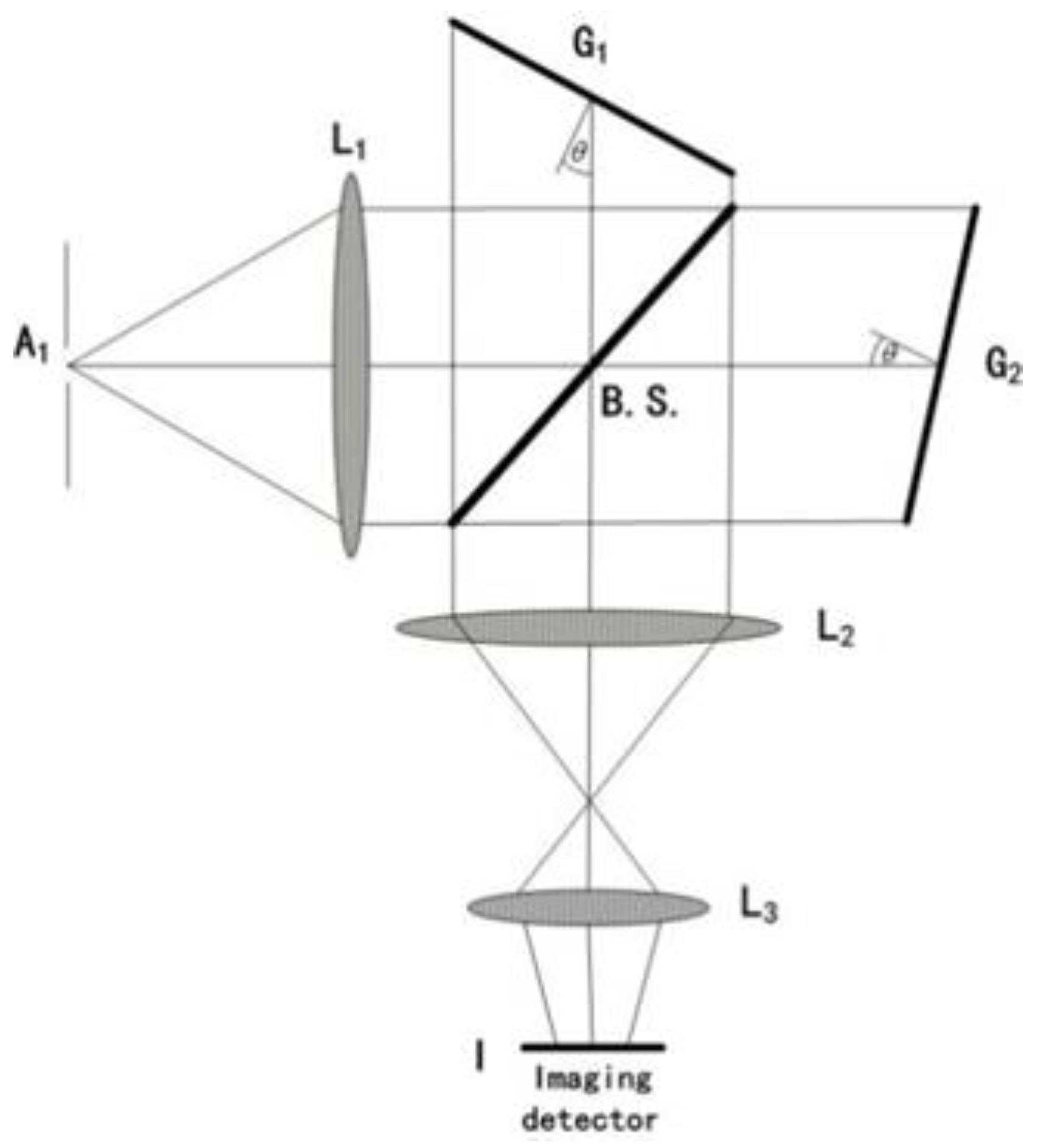
2.1. SHS Technology
2.2. GMI Specifications
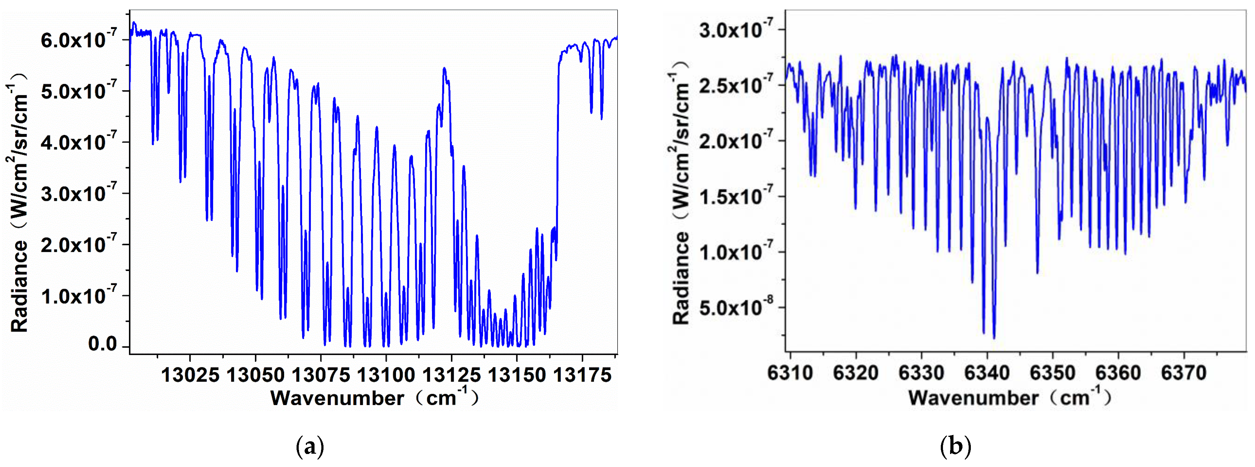
2.3. Recovery of Spectral Interferograms
3. Retrieval Method
3.1. Forward Model
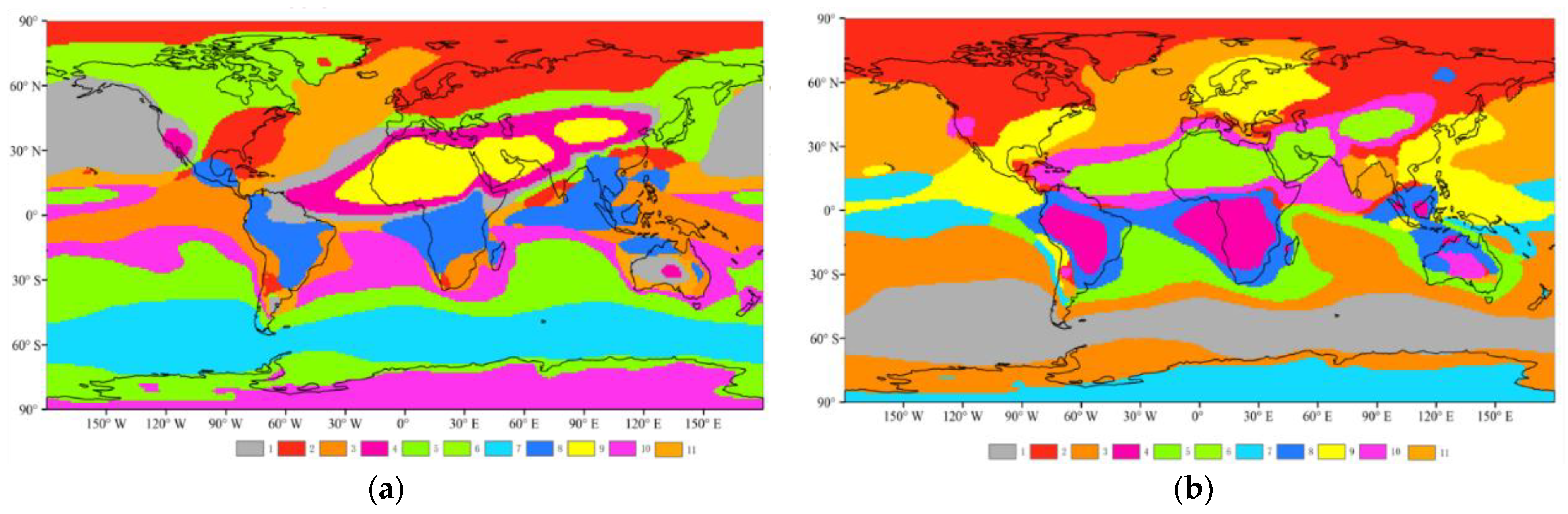
3.2. State Vectors and Auxiliary Parameters
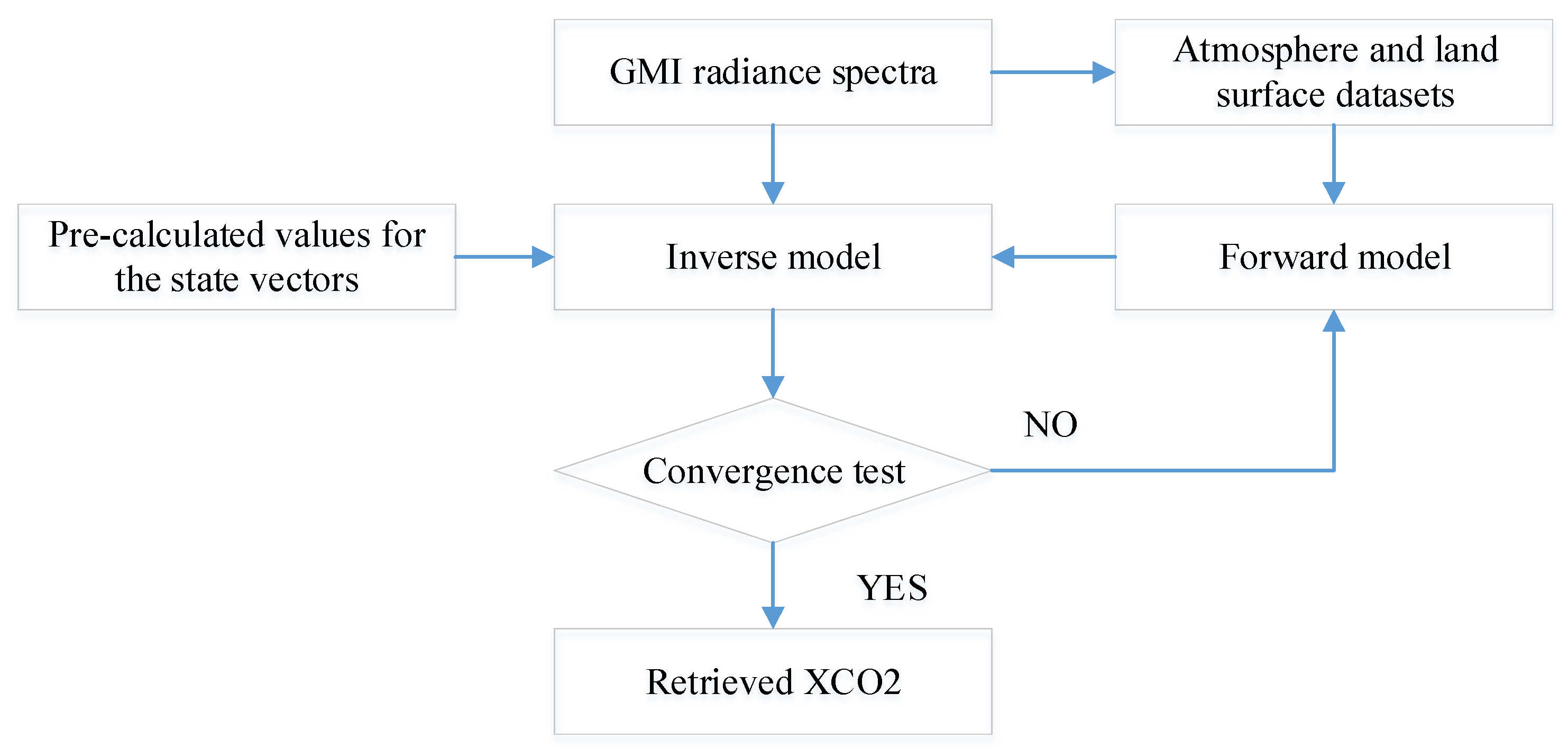
3.3. Retrieval Algorithm
4. Simulated Analyses
4.1. Simulations of GMI Observations
4.2. Retrieval Results
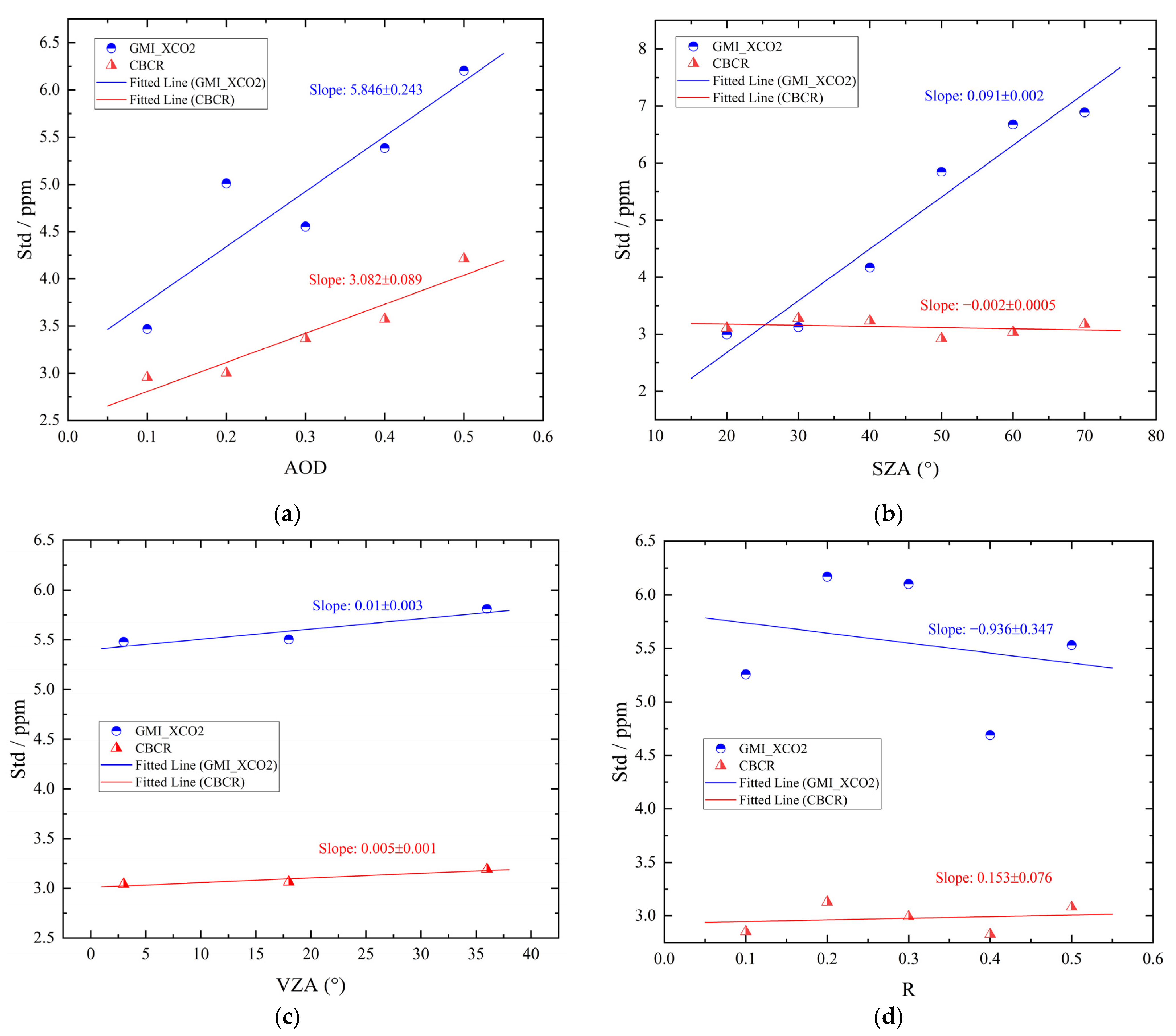
5. Validation
5.1. Data Preparation
5.2. Retrieval Results and Validation
6. Conclusions
Author Contributions
Funding
Institutional Review Board Statement
Informed Consent Statement
Data Availability Statement
Acknowledgments
Conflicts of Interest
References
- Eldering, A.; Wennberg, P.O.; Crisp, D.; Schimel, D.S.; Gunson, M.R.; Chatterjee, A.; Liu, J.; Schwandner, F.M.; Sun, Y.; O’Dell, C.W.; et al. The Orbiting Carbon Observatory-2 early science investigations of regional carbon dioxide fluxes. Science 2017, 358. [Google Scholar] [CrossRef] [Green Version]
- Boesch, H.; Baker, D.; Connor, B.; Crisp, D.; Miller, C. Global characterization of CO2 column retrievals from shortwave-infrared satellite observations of the Orbiting Carbon Observatory-2 mission. Remote Sens. 2011, 3, 270–304. [Google Scholar] [CrossRef] [Green Version]
- Zhang, X.; Wang, F.; Wang, W.; Huang, F.; Chen, B.; Gao, L.; Wang, S.; Yan, H.; Ye, H.; Si, F.; et al. The development and application of satellite remote sensing for atmospheric compositions in China. Atmos. Res. 2020, 245, 105056. [Google Scholar] [CrossRef]
- Rayner, P.J.; O’Brien, D.M. The utility of remotely sensed CO2 concentration data in surface source inversions. Geophys. Res. Lett. 2001, 28, 175–178. [Google Scholar] [CrossRef] [Green Version]
- Houweling, S.; Breon, F.-M.; Aben, I.; Rödenbeck, C.; Gloor, M.; Heimann, M.; Ciais, P. Inverse modeling of CO 2 sources and sinks using satellite data: A synthetic inter-comparison of measurement techniques and their performance as a function of space and time. Atmos. Chem. Phys. 2004, 4, 523–538. [Google Scholar] [CrossRef] [Green Version]
- Buchwitz, M.; Reuter, M.; Noël, S.; Bramstedt, K.; Schneising, O.; Hilker, M.; Fuentes Andrade, B.; Bovensmann, H.; Burrows, J.P.; Di Noia, A. Can a regional-scale reduction of atmospheric CO2 during the COVID-19 pandemic be detected from space? A case study for East China using satellite XCO2 retrievals. Atmos. Meas. Tech. 2021, 14, 2141–2166. [Google Scholar] [CrossRef]
- Eldering, A.; O’Dell, C.W.; Wennberg, P.O.; Crisp, D.; Gunson, M.R.; Viatte, C.; Avis, C.; Braverman, A.; Castano, R.; Chang, A. The Orbiting Carbon Observatory-2: First 18 months of science data products. Atmos. Meas. Tech. 2017, 10, 549–563. [Google Scholar] [CrossRef] [Green Version]
- Liang, A.; Gong, W.; Han, G.; Xiang, C. Comparison of satellite-observed XCO2 from GOSAT, OCO-2, and ground-based TCCON. Remote Sens. 2017, 9, 1033. [Google Scholar] [CrossRef] [Green Version]
- Shi, H.; Li, Z.; Ye, H.; Luo, H.; Xiong, W.; Wang, X. First level 1 product results of the greenhouse gas monitoring instrument on the GaoFen-5 satellite. IEEE Trans. Geosci. Remote Sens. 2020, 59, 899–914. [Google Scholar] [CrossRef]
- Wu, H. Error analysis of the greenhouse-gases monitor instrument short wave infrared XCO2 retrieval algorithm. J. Appl. Remote Sens. 2018, 12, 1. [Google Scholar] [CrossRef]
- Aben, I.; Hasekamp, O.; Hartmann, W. Uncertainties in the space-based measurements of CO2 columns due to scattering in the Earth’s atmosphere. J. Quant. Spectrosc. Radiat. Transf. 2007, 104, 450–459. [Google Scholar] [CrossRef]
- Maksyutov, S.; Valsala, V. Algorithms for Carbon Flux Estimation Using GOSAT Observational Data; Center for Global Environmental Research, National Institute for Environmental Studies: Tsukuba, Japan, 2010; Volume 15, pp. 1–112. [Google Scholar]
- Meister, G. Bidirectional Reflectance of Urban Surfaces. Ph.D. Thesis, Staats-und Universitätsbibliothek Hamburg Carl von Ossietzky, Hamburg, Germany, 2000. [Google Scholar]
- Gastellu-Etchegorry, J.P.; Martin, E.; Gascon, F. DART: A 3D model for simulating satellite images and studying surface radiation budget. Int. J. Remote Sens. 2004, 25, 73–96. [Google Scholar] [CrossRef]
- Xu, F.; Sun, L. The BRDF Model Construction and Application in Urban Areas. In Advances in Computer Science and Engineering; Springer: Berlin/Heidelberg, Germany, 2012; pp. 379–386. [Google Scholar]
- O’dell, C.W.; Eldering, A.; Wennberg, P.O.; Crisp, D.; Gunson, M.R.; Fisher, B.; Frankenberg, C.; Kiel, M.; Lindqvist, H.; Mandrake, L. Improved retrievals of carbon dioxide from Orbiting Carbon Observatory-2 with the version 8 ACOS algorithm. Atmos. Meas. Tech. 2018, 11, 6539–6576. [Google Scholar] [CrossRef] [Green Version]
- Connor, B.; Bösch, H.; McDuffie, J.; Taylor, T.; Fu, D.; Frankenberg, C.; O’Dell, C.; Payne, V.H.; Gunson, M.; Pollock, R. Quantification of uncertainties in OCO-2 measurements of XCO 2: Simulations and linear error analysis. Atmos. Meas. Tech. 2016, 9, 5227–5238. [Google Scholar] [CrossRef] [Green Version]
- Yoshida, Y.; Ota, Y.; Eguchi, N.; Kikuchi, N.; Nobuta, K.; Tran, H.; Morino, I.; Yokota, T. Retrieval algorithm for CO 2 and CH 4 column abundances from short-wavelength infrared spectral observations by the Greenhouse gases observing satellite. Atmos. Meas. Tech. 2011, 4, 717–734. [Google Scholar] [CrossRef] [Green Version]
- O’Dell, C.W.; Connor, B.; Bösch, H.; O’Brien, D.; Frankenberg, C.; Castano, R.; Christi, M.; Eldering, D.; Fisher, B.; Gunson, M. The ACOS CO 2 retrieval algorithm–Part 1: Description and validation against synthetic observations. Atmos. Meas. Tech. 2012, 5, 99–121. [Google Scholar] [CrossRef] [Green Version]
- Roesler, F.L.; Harlander, J.M. Spatial heterodyne spectroscopy: Interferometric performance at any wavelength without scanning. In Proceedings of the Optical Spectroscopic Instrumentation and Techniques for the 1990s: Applications in Astronomy, Chemistry, and Physics; International Society for Optics and Photonics: Bellingham, WA, USA, 1990; Volume 1318, pp. 234–243. [Google Scholar]
- Rozanov, V.V.; Dinter, T.; Rozanov, A.V.; Wolanin, A.; Bracher, A.; Burrows, J.P. Radiative transfer modeling through terrestrial atmosphere and ocean accounting for inelastic processes: Software package SCIATRAN. J. Quant. Spectrosc. Radiat. Transf. 2017, 194, 65–85. [Google Scholar] [CrossRef] [Green Version]
- Thuillier, G.; Hersé, M.; Foujols, T.; Peetermans, W.; Gillotay, D.; Simon, P.C.; Mandel, H. The solar spectral irradiance from 200 to 2400 nm as measured by the SOLSPEC spectrometer from the ATLAS and EURECA missions. Sol. Phys. 2003, 214, 1–22. [Google Scholar] [CrossRef]
- Toon, G.C. Solar Line List for GGG2014, TCCON Data Archive; Solar. R0/1221658; The Carbon Dioxide Information Analysis Center, Oak Ridge National Laboratory: Oak Ridge, TN, USA, 2014. [Google Scholar] [CrossRef]
- Schaaf, C.B.; Gao, F.; Strahler, A.H.; Lucht, W.; Li, X.; Tsang, T.; Strugnell, N.C.; Zhang, X.; Jin, Y.; Muller, J.P.; et al. First operational BRDF, albedo nadir reflectance products from MODIS. Remote Sens. Environ. 2002, 83, 135–148. [Google Scholar] [CrossRef] [Green Version]
- Taylor, M.; Kazadzis, S.; Amiridis, V.; Kahn, R.A. Global aerosol mixtures and their multiyear and seasonal characteristics. Atmos. Environ. 2015, 116, 112–129. [Google Scholar] [CrossRef]
- Ginoux, P.; Chin, M.; Tegen, I.; Prospero, J.M.; Holben, B.; Dubovik, O.; Lin, S. Sources and distributions of dust aerosols simulated with the GOCART model. J. Geophys. Res. Atmos. 2001, 106, 20255–20273. [Google Scholar] [CrossRef]
- Bey, I.; Jacob, D.J.; Yantosca, R.M.; Logan, J.A.; Field, B.D.; Fiore, A.M.; Li, Q.; Liu, H.Y.; Mickley, L.J.; Schultz, M.G. Global modeling of tropospheric chemistry with assimilated meteorology: Model description and evaluation. J. Geophys. Res. Atmos. 2001, 106, 23073–23095. [Google Scholar] [CrossRef]
- Chan, K.L. Aerosol optical depths and their contributing sources in Taiwan. Atmos. Environ. 2017, 148, 364–375. [Google Scholar] [CrossRef]
- Eguchi, N.; Saito, R.; Saeki, T.; Nakatsuka, Y.; Belikov, D.; Maksyutov, S. A priori covariance estimation for CO2 and CH4 retrievals. J. Geophys. Res. Atmos. 2010, 115. [Google Scholar] [CrossRef]
- Ye, H.; Wang, X.; Wu, J.; Jiang, Y. A priori estimation for spectral shift of atmospheric carbon dioxide satellite measurement. Optik (Stuttg) 2018, 158, 283–290. [Google Scholar] [CrossRef]
- Gorokhovich, Y.; Voustianiouk, A. Accuracy assessment of the processed SRTM-based elevation data by CGIAR using field data from USA and Thailand and its relation to the terrain characteristics. Remote Sens. Environ. 2006, 104, 409–415. [Google Scholar] [CrossRef]
- Rodgers, C.D. Inverse Methods for Atmospheric Sounding: Theory and Practice; World Scientific: Singapore, 2000; Volume 2, ISBN 9814498688. [Google Scholar]
- Li, C.; Ma, J.; Yang, P.; Li, Z. Detection of cloud cover using dynamic thresholds and radiative transfer models from the polarization satellite image. J. Quant. Spectrosc. Radiat. Transf. 2019, 222–223, 196–214. [Google Scholar] [CrossRef]
- Wunch, D.; Toon, G.C.; Wennberg, P.O.; Wofsy, S.C.; Stephens, B.B.; Fischer, M.L.; Uchino, O.; Abshire, J.B.; Bernath, P.; Biraud, S.C. Calibration of the Total Carbon Column Observing Network using aircraft profile data. Atmos. Meas. Tech. 2010, 3, 1351–1362. [Google Scholar] [CrossRef] [Green Version]
- Wunch, D.; Toon, G.C.; Blavier, J.-F.L.; Washenfelder, R.A.; Notholt, J.; Connor, B.J.; Griffith, D.W.T.; Sherlock, V.; Wennberg, P.O. The total carbon column observing network. Philos. Trans. R. Soc. A Math. Phys. Eng. Sci. 2011, 369, 2087–2112. [Google Scholar] [CrossRef] [PubMed] [Green Version]


| Parameter | Spectral Band | |||
|---|---|---|---|---|
| NIR | SWIR-1 | SWIR-2 | SWIR-3 | |
| Spectral range (nm) | 759–769 | 1568–1583 | 1642–1658 | 2043–2058 |
| Spectral resolution at FWHM (nm) | 0.035 | 0.067 | 0.067 | 0.113 |
| Signal-to-noise ratio (SNR) | 300 | 300 | 250 | 250 |
| Spatial resolution | 10.5 km × 10.5 km | |||
| Data coverage | August 2018 to April 2020 | |||
| Spring | Component | Case1 | Case2 | Case3 | Case4 | Case5 | Case6 | Case7 | Case8 | Case9 | Case 10 | Case 11 |
| Biomass burning (%) | 12.3 | 9.5 | 16.4 | 9.6 | 6.5 | 10.1 | 3.5 | 40.1 | 4.2 | 9.2 | 12.4 | |
| Sulfate (%) | 34.7 | 55.8 | 66.5 | 24.7 | 39.3 | 47 | 24.8 | 45.1 | 9.5 | 49.8 | 43.3 | |
| Dust (%) | 41.5 | 28.7 | 4.3 | 62.5 | 4.1 | 38 | 2.8 | 9.1 | 85.6 | 4.1 | 26.4 | |
| Sea salt (%) | 11.5 | 6.1 | 12.8 | 3.2 | 50.1 | 5 | 68.9 | 5.6 | 0.7 | 36.9 | 17.9 | |
| Black carbon (%) | 3.2 | 2.7 | 3.5 | 2.6 | 1.7 | 2.9 | 0.9 | 6.9 | 1.3 | 2.3 | 3.5 | |
| Organic carbon (%) | 9.1 | 6.8 | 12.9 | 7 | 4.8 | 7.2 | 2.6 | 33.2 | 2.9 | 6.9 | 8.9 | |
| Summer | Component | Case1 | Case2 | Case3 | Case4 | Case5 | Case6 | Case7 | Case8 | Case9 | Case 10 | Case 11 |
| Biomass burning (%) | 7.6 | 21 | 11.8 | 72 | 24.4 | 5 | 8.9 | 41.6 | 14.7 | 14.7 | 12.7 | |
| Sulfate (%) | 20.3 | 50.7 | 32 | 22.8 | 35.4 | 16.5 | 49 | 37 | 67 | 32.9 | 52.1 | |
| Dust (%) | 2.2 | 26.5 | 2.8 | 2.7 | 5.8 | 76.7 | 2.8 | 11.2 | 11.1 | 46.6 | 25.1 | |
| Sea salt (%) | 69.9 | 1.8 | 53.4 | 2.5 | 34.4 | 1.8 | 39.2 | 10.1 | 7.3 | 5.8 | 10.1 | |
| Black carbon (%) | 1.4 | 4.3 | 2.7 | 11.4 | 4.9 | 1.7 | 2.1 | 7.3 | 3.6 | 3.6 | 3.8 | |
| Organic carbon (%) | 6.2 | 16.7 | 9.1 | 60.6 | 19.4 | 3.3 | 6.8 | 34.3 | 11 | 11.1 | 9 | |
| Autumn | Component | Case1 | Case2 | Case3 | Case4 | Case5 | Case6 | Case7 | Case8 | Case9 | Case 10 | Case11 |
| Biomass burning (%) | 15.2 | 9.1 | 11.4 | 21.9 | 13.4 | 61.4 | 37.8 | 13.2 | 14.2 | 17.6 | 5.2 | |
| Sulfate (%) | 24.2 | 43.9 | 62.1 | 35.6 | 52.2 | 28.7 | 37 | 57.2 | 30.5 | 71 | 13.3 | |
| Dust (%) | 4.4 | 21.4 | 19.2 | 5.4 | 26.9 | 6.1 | 7.8 | 2.8 | 51.2 | 4.6 | 80.3 | |
| Sea salt (%) | 56.2 | 25.6 | 7.3 | 37.1 | 7.5 | 3.8 | 17.3 | 26.7 | 4.1 | 6.8 | 1.1 | |
| Black carbon (%) | 2.4 | 3.4 | 3.5 | 4 | 4.1 | 10 | 7.2 | 3.3 | 3.8 | 4.4 | 1.7 | |
| Organic carbon (%) | 12.7 | 5.8 | 7.9 | 17.9 | 9.2 | 51.4 | 30.6 | 9.9 | 10.4 | 13.2 | 3.6 | |
| Winter | Component | Case1 | Case2 | Case3 | Case4 | Case5 | Case6 | Case7 | Case8 | Case9 | Case10 | |
| Biomass burning (%) | 53.9 | 10.9 | 7.5 | 6.5 | 15 | 12.6 | 14.4 | 9 | 31.2 | 7.8 | ||
| Sulfate (%) | 25.9 | 50.9 | 58 | 37.9 | 24.5 | 64.7 | 42.8 | 42 | 53.9 | 10.5 | ||
| Dust (%) | 16.5 | 5.9 | 18.2 | 6.4 | 56.1 | 5.7 | 35.8 | 18.1 | 6.8 | 80.7 | ||
| Sea salt (%) | 3.7 | 32.3 | 16.3 | 49.2 | 4.5 | 16.9 | 7.1 | 30.9 | 8.1 | 1.1 | ||
| Black carbon (%) | 7.5 | 2.6 | 3 | 1.6 | 3.7 | 2.9 | 4.5 | 3 | 6.4 | 2 | ||
| Organic carbon (%) | 46.4 | 8.3 | 4.5 | 4.9 | 11.2 | 9.8 | 9.9 | 6 | 24.8 | 5.8 |
| State Vectors | Auxiliary Parameters |
|---|---|
| CO2 Profile (ppm) | Aerosol Type |
| SWIR-1 band kernel parameters | Surface Height (km) |
| NIR and SWIR-3 Band Albedo | Pressure Profile (hPa) |
| AOD @550nm | H2O Profile (ppm) |
| Wavenumber Correction Factors | Temperature Profile (K) |
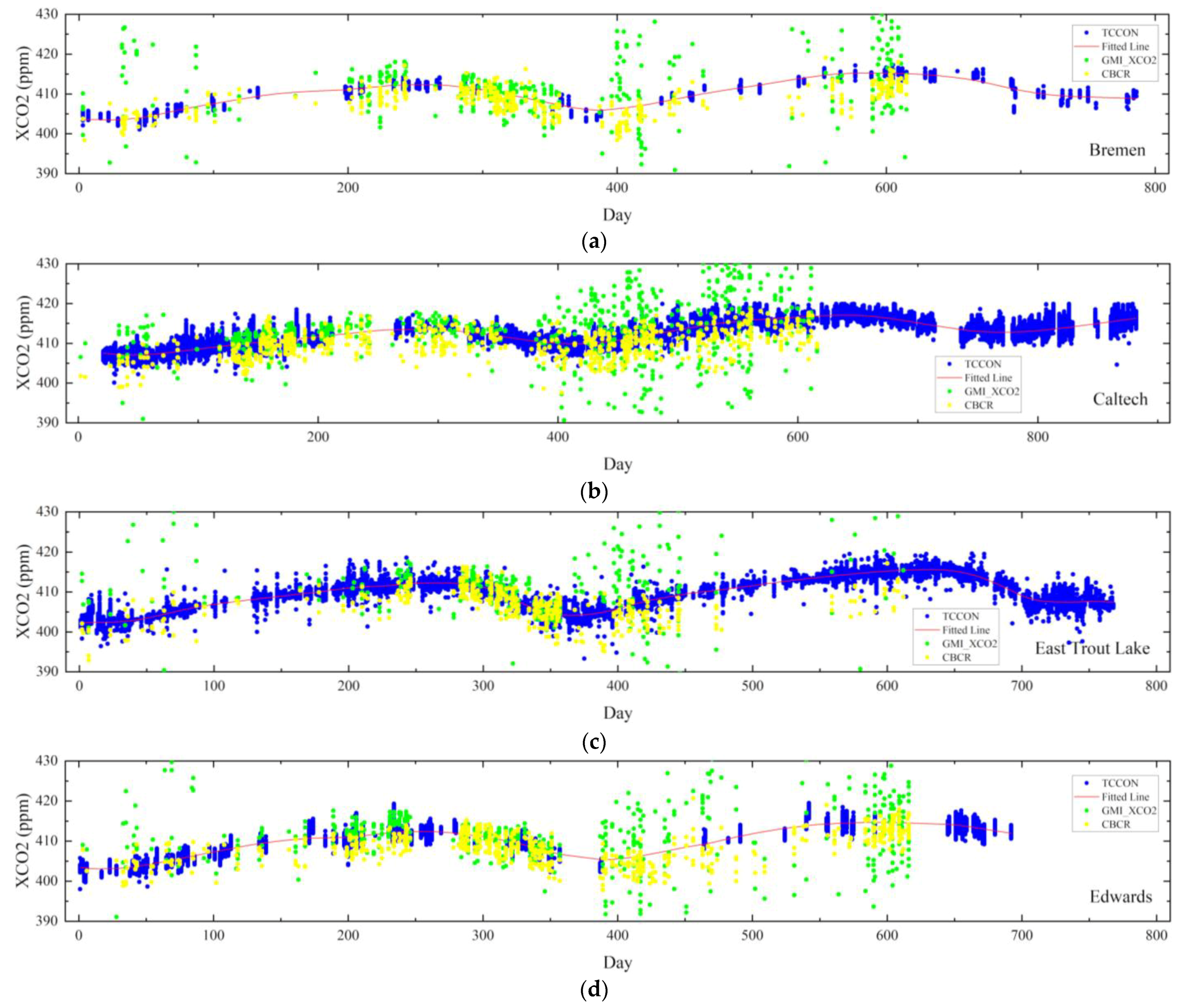
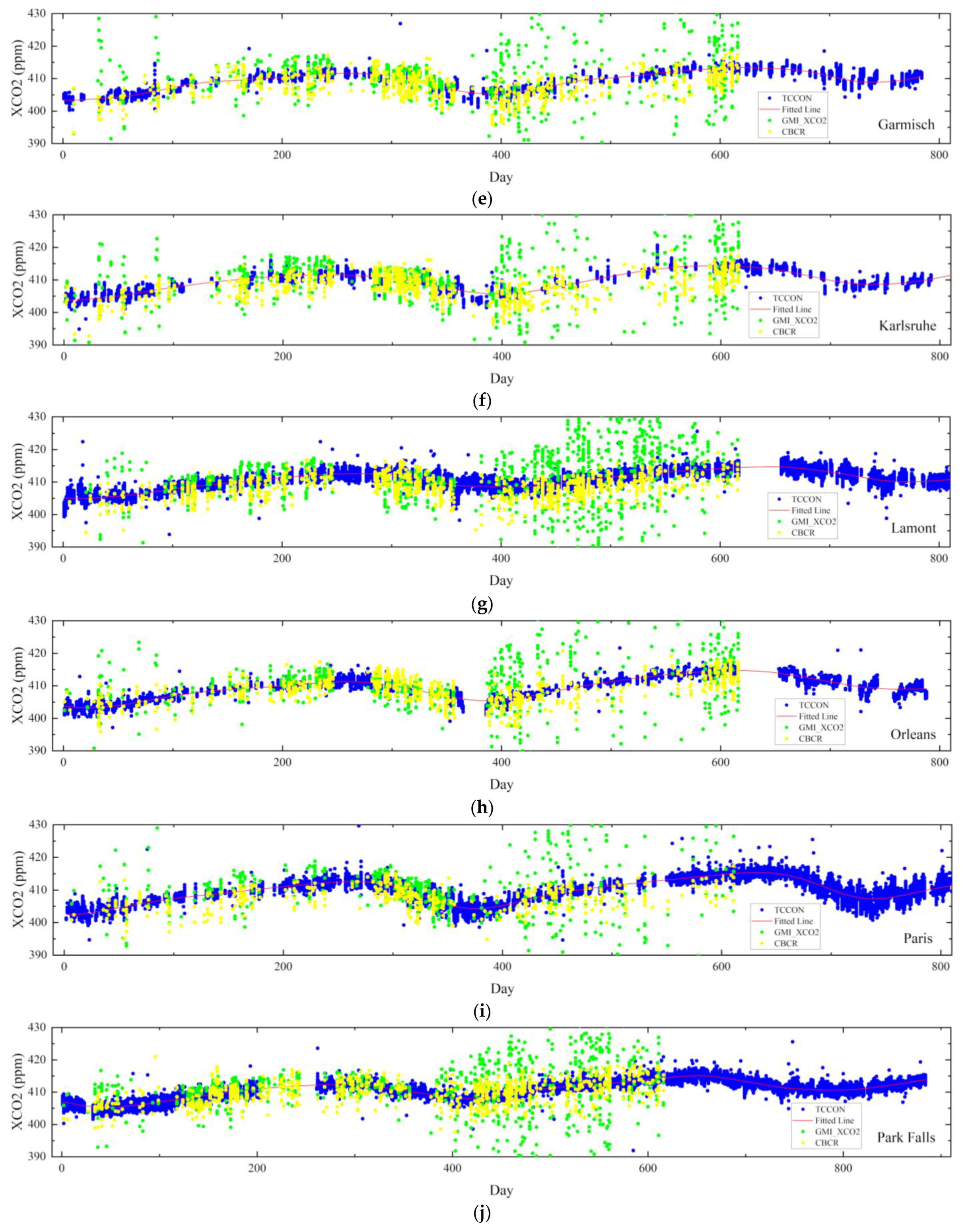
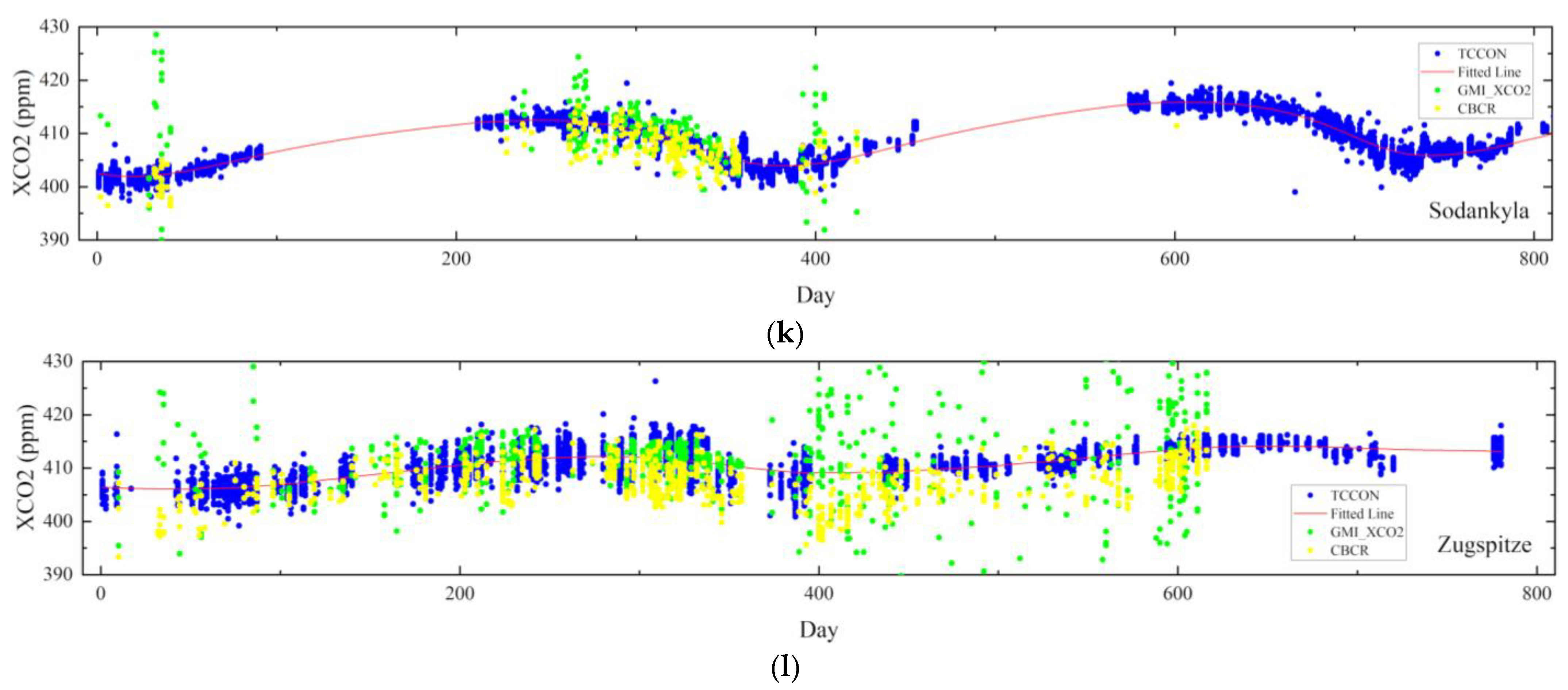
| Sites | GMI_XCO2 & TCCON | CBCR & TCCON |
|---|---|---|
| Sodankyla | 37.36% | 76.8% |
| East Trout Lake | 37.42% | 63.55% |
| Bremen | 30.32% | 70.5% |
| Karlsruhe | 34.94% | 61.98% |
| Paris | 30.93% | 45.75% |
| Orleans | 25.39% | 69.02% |
| Garmisch | 28.34% | 63.45% |
| Zugspitze | 24.18% | 54.94% |
| Park Falls | 24.85% | 51.8% |
| Lamont | 17.05% | 60.87% |
| Caltech | 28.88% | 55.9% |
| Edwards | 32.59% | 73.77% |
| Sites | Lat/° | Lon/° | GMI_XCO2 | CBCR | ||
|---|---|---|---|---|---|---|
| Mean Deviation/ppm | Standard Deviation/ppm | Mean Deviation/ppm | Standard Deviation/ppm | |||
| Sodankyla | 67.37 | 26.63 | 0.23 | 5.49 | −1.38 | 2.77 |
| East Trout Lake | 54.35 | −104.99 | 0.26 | 4.48 | −1.67 | 3.30 |
| Bremen | 53.1 | 8.85 | 0.17 | 5.79 | −2.14 | 3.03 |
| Karlsruhe | 49.1 | 8.44 | 0.51 | 5.72 | −0.80 | 2.96 |
| Paris | 48.97 | 2.37 | 1.16 | 3.58 | −0.82 | 2.43 |
| Orleans | 47.97 | 2.11 | 1.27 | 5.63 | −0.47 | 3.02 |
| Garmisch | 47.48 | 11.06 | 1.21 | 6.20 | −1.24 | 3.16 |
| Zugspitze | 47.42 | 10.98 | 0.51 | 5.42 | −2.38 | 3.12 |
| Park Falls | 45.94 | −90.27 | −0.56 | 5.01 | −1.53 | 3.29 |
| Lamont | 36.6 | −97.49 | 0.21 | 6.06 | −2.68 | 2.88 |
| Caltech | 34.14 | −118.13 | 1.01 | 6.01 | −1.51 | 2.87 |
| Edwards | 34.96 | −117.88 | 0.60 | 5.85 | −0.26 | 3.16 |
| Total | 0.58 | 5.64 | −1.33 | 3.13 | ||
Publisher’s Note: MDPI stays neutral with regard to jurisdictional claims in published maps and institutional affiliations. |
© 2022 by the authors. Licensee MDPI, Basel, Switzerland. This article is an open access article distributed under the terms and conditions of the Creative Commons Attribution (CC BY) license (https://creativecommons.org/licenses/by/4.0/).
Share and Cite
Ye, H.; Shi, H.; Li, C.; Wang, X.; Xiong, W.; An, Y.; Wang, Y.; Liu, L. A Coupled BRDF CO2 Retrieval Method for the GF-5 GMI and Improvements in the Correction of Atmospheric Scattering. Remote Sens. 2022, 14, 488. https://doi.org/10.3390/rs14030488
Ye H, Shi H, Li C, Wang X, Xiong W, An Y, Wang Y, Liu L. A Coupled BRDF CO2 Retrieval Method for the GF-5 GMI and Improvements in the Correction of Atmospheric Scattering. Remote Sensing. 2022; 14(3):488. https://doi.org/10.3390/rs14030488
Chicago/Turabian StyleYe, Hanhan, Hailiang Shi, Chao Li, Xianhua Wang, Wei Xiong, Yuan An, Yue Wang, and Liangchen Liu. 2022. "A Coupled BRDF CO2 Retrieval Method for the GF-5 GMI and Improvements in the Correction of Atmospheric Scattering" Remote Sensing 14, no. 3: 488. https://doi.org/10.3390/rs14030488
APA StyleYe, H., Shi, H., Li, C., Wang, X., Xiong, W., An, Y., Wang, Y., & Liu, L. (2022). A Coupled BRDF CO2 Retrieval Method for the GF-5 GMI and Improvements in the Correction of Atmospheric Scattering. Remote Sensing, 14(3), 488. https://doi.org/10.3390/rs14030488