Article

Estimation of Forest Aboveground Biomass of Two Major Conifers in Ibaraki Prefecture, Japan, from PALSAR-2 and Sentinel-2 Data

1
Graduate School of Agriculture, Hokkaido University, Sapporo 060-8589, Hokkaido, Japan
2
Research Faculty of Agriculture, Hokkaido University, Sapporo 060-8589, Hokkaido, Japan
3
Global Center for Food, Land and Water Resources, Research Faculty of Agriculture, Hokkaido University, Sapporo 060-8589, Hokkaido, Japan
4
Earth Observation Research Center, Japan Aerospace Exploration Agency (JAXA), Tsukuba 305-8505, Ibaraki, Japan
5
College of Ecology and Environment, Hainan University, Haiko 570228, China
*
Author to whom correspondence should be addressed.
Remote Sens. 2022, 14(3), 468; https://doi.org/10.3390/rs14030468
Submission received: 13 December 2021 / Revised: 14 January 2022 / Accepted: 14 January 2022 / Published: 19 January 2022
(This article belongs to the Special Issue ALOS-2/PALSAR-2 Calibration, Validation, Science and Applications)

Abstract

:
Forest biomass is a crucial component of the global carbon budget in climate change studies. Therefore, it is essential to develop a credible way to estimate forest biomass as carbon stock. Our study used PALSAR-2 (ALOS-2) and Sentinel-2 images to drive the Random Forest regression model, which we trained with airborne lidar data. We used the model to estimate forest aboveground biomass (AGB) of two significant coniferous trees, Japanese cedar and Japanese cypress, in Ibaraki Prefecture, Japan. We used 48 variables derived from the two remote sensing datasets to predict forest AGB under the Random Forest algorithm, and found that the model that combined the two datasets performed better than models based on only one dataset, with R2 = 0.31, root-mean-square error (RMSE) = 54.38 Mg ha−1, mean absolute error (MAE) = 40.98 Mg ha−1, and relative RMSE (rRMSE) of 0.35 for Japanese cedar, and R2 = 0.37, RMSE = 98.63 Mg ha−1, MAE = 76.97 Mg ha−1, and rRMSE of 0.33 for Japanese cypress, over the whole AGB range. In the satellite AGB map, the total AGB of Japanese cedar in 17 targeted cities in Ibaraki Prefecture was 5.27 Pg, with a mean of 146.50 Mg ha−1 and a standard deviation of 44.37 Mg ha−1. The total AGB of Japanese cypress was 3.56 Pg, with a mean of 293.12 Mg ha−1 and a standard deviation of 78.48 Mg ha−1. We also found a strong linear relationship with between the model estimates and Japanese government data, with R2 = 0.99 for both species and found the government information underestimates the AGB for cypress but overestimates it for cedar. Our results reveal that combining information from multiple sensors can predict forest AGB with increased accuracy and robustness.

1. Introduction

Forests play a significant role in the global carbon budget, as they store a large share of terrestrial carbon in their biomass [1]. About 90% of the total carbon in the world’s vegetation stock comprises forests, which cover 65% of the land area [2]. The forest aboveground biomass (AGB) is therefore considered one of the most important factors in evaluating forest carbon pools [3]. To better understand the amount of stored carbon in forest, spatially explicit and temporally consistent estimates of AGB are urgently needed [4]. Field biometric studies to quantify AGB, usually using the diameter at breast height (DBH) and tree height as inputs for allometries based on destructive sampling, have provided simple and useful models, but constructing reliable allometric relationships over large areas is difficult, time-consuming, and expensive [5].
Remote sensing techniques can be scaled up to cover large areas, thereby allowing efficient collection of forest biophysical information and repeated analysis to reveal changes over time [6]. Among the available techniques, lidar (light detection and ranging) is one of the most accurate remote-sensing technologies for assessing forest canopy characteristics [7]. Lidar data are particularly useful for mapping vertical structural attributes of ecosystems such as carbon storage, biomass, and stand volume [8]. These advantages let lidar-based approaches provide high-quality assessment of AGB, even in forests with high biomass per unit area, and can retrieve numerous forest parameters in a single survey [9,10,11].
Despite the ability of airborne lidar to provide highly accurate assessments of parameters such as tree density at an urban scale, the high cost of airborne lidar data can prevent its use in larger areas [12]. In addition, the sparse coverage of land areas by space-borne lidar (e.g., ICESat2, GEDI) reduces the availability of these data for large-area estimation of forest AGB. This suggests the need to develop a robust and consistent large-area model for AGB estimation that takes advantage of airborne lidar datasets, but combines them with other data sources to perform estimation over long time periods and large areas [13]. Studies often use two main sources of AGB training data based on ground-truthing (e.g., forest inventory data) and airborne lidar [14].
Synthetic aperture radar (SAR) provides information on the dielectric (essentially, moisture content) and structural properties of the targeted objects, which include soil surfaces and plants in wetlands, agricultural land, and forests [15,16,17]. However, when estimating forest AGB, this kind of dataset depends on the degree of saturation, which refers to the AGB level at which the signal’s sensitivity (e.g., backscatter, reflectance) becomes too small to be measurable or where the signal fails to penetrate the forest canopy [18]. These phenomena lead to drastic deterioration of accuracy at high levels of AGB. Thus, saturation levels limit the role that SAR sensors can play in direct measurement of forest biomass for global inventories [19].
One strategy that can be used to overcome this problem is to combine SAR images with optical images [20]. Multispectral optical imagery contains information on the photosynthetic parts of the vegetation, which are rich in chlorophyll, and optical satellite images have a long history of being used for estimation of forest parameters and assessment of different wood quality results. Unfortunately, optical satellite signals are strongly affected by weather and other atmospheric conditions; under unsuitable conditions, optical images are prone to significant errors [21]. Another drawback is that optical satellite signals cannot measure vegetation structure directly and suffer from spectral saturation in densely vegetated environments, which limits their ability to map AGB in some cases, as is the case for SAR data [22]. However, because the two kinds of satellite data have different limitations, it may be possible to combine them to estimate forest AGB, with the advantages of one method offsetting the disadvantages of the other. Selection of appropriate regression models for modeling AGB is crucial because optical remote sensing data and SAR data have different relationships with AGB. For example, some studies have shown a strong linear relationship between SAR and AGB [23,24]. Other studies found that non-linear regression models provided a better fit for this relationship [25,26]. Because of these contradictory results, it is worth considering alternatives to simple regression.
Here, we selected the Random Forest regression model because it has worked well with both SAR data [27] and optical satellite data [28]. Random Forest is an efficient machine learning method proposed by Breiman [29]. It is a type of ensemble machine learning algorithm based on bootstrap aggregation also called bagging [29]. The model lets researchers combine different sources of satellite images in a single model [30]. It is well suited to analyzing complex non-linear and possibly hierarchical interactions in large datasets [31]. Moreover, it can determine the importance of the variables to provide a plausible strategy for combining variables from different datasets. This approach has been used successfully in many cases with different combinations of satellite datasets [32,33,34].
Although Random Forest estimates AGB well, it tends to overestimate AGB at low values of AGB and underestimate it at high values [35]. Despite these limitations, many researchers have estimated forest AGB in different countries by using SAR and optical satellite datasets, including Mexico, China, Russia, the USA, and Cameroon [11,36,37,38,39]. However, few areas have been studied using Random Forest in Japan [40]. To provide more data on this approach, we selected two species of forest tree as our targets. Japanese cedar (Cryptomeria japonica) and Japanese cypress (Chamaecyparis obtusa) play important roles in Japanese forest ecosystems, and cover 28% of the forested area in Japan, which is equivalent to 19% of Japan’s land surface [41].
Our objectives here were to:
(1)
assess the potential of combining two types of satellite data (SAR and optical sensors) to improve AGB estimation performance;
(2)
estimate the spatial extent of forest AGB for two major forest types in northern Ibaraki Prefecture, Japan; and
(3)
benchmark the AGB estimates using forest register data collected by the Ibaraki Prefecture government.

2. Materials and Methods
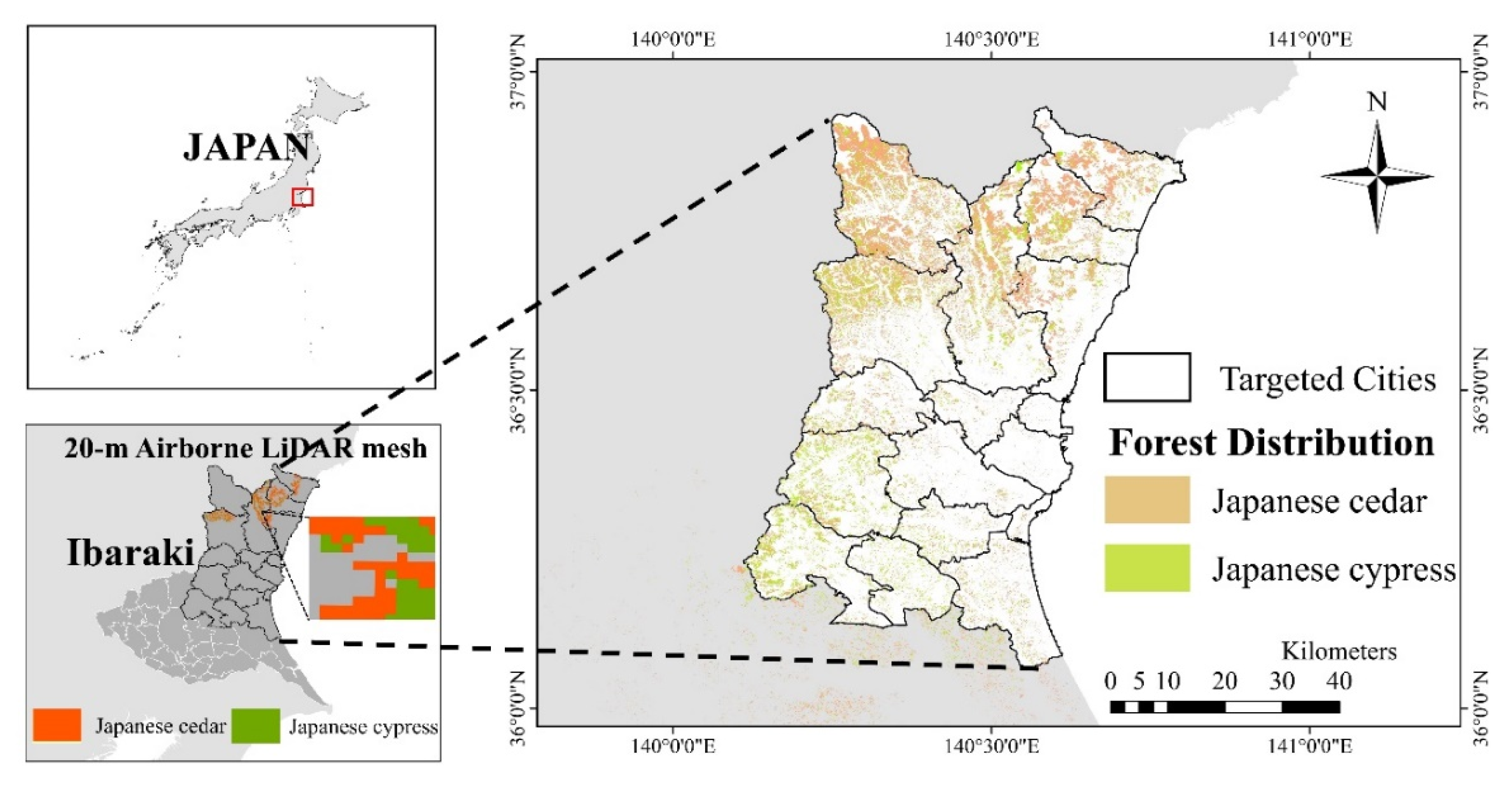
2.1. Study Area

We focused on plantations of two forest tree species, both in the cypress family (Cupressaceae), growing in Japan’s Ibaraki Prefecture, central Japan. The prefecture has an active forest industry, supported by C. japonica and C. obtusa. These are major plantation species throughout Japan, occupying 4.44 × 10⁶ and 2.60 × 10⁶ ha of forest (equivalent to 18% and 10% of the forest area in Japan), respectively [41]. Both are important timber resources, and are also associated with public functions such as conservation of natural land, prevention of global warming, and recharge of water sources.
Our study area was located in northern Ibaraki Prefecture, which is the prefecture’s main forest area. The southern part of the prefecture is dominated by agricultural land with almost no forests (Figure 1). The regional average elevation is 22 m above sea level and the highest point is 1021 m, with rugged terrain; the target forests are distributed mainly in mountainous topography.

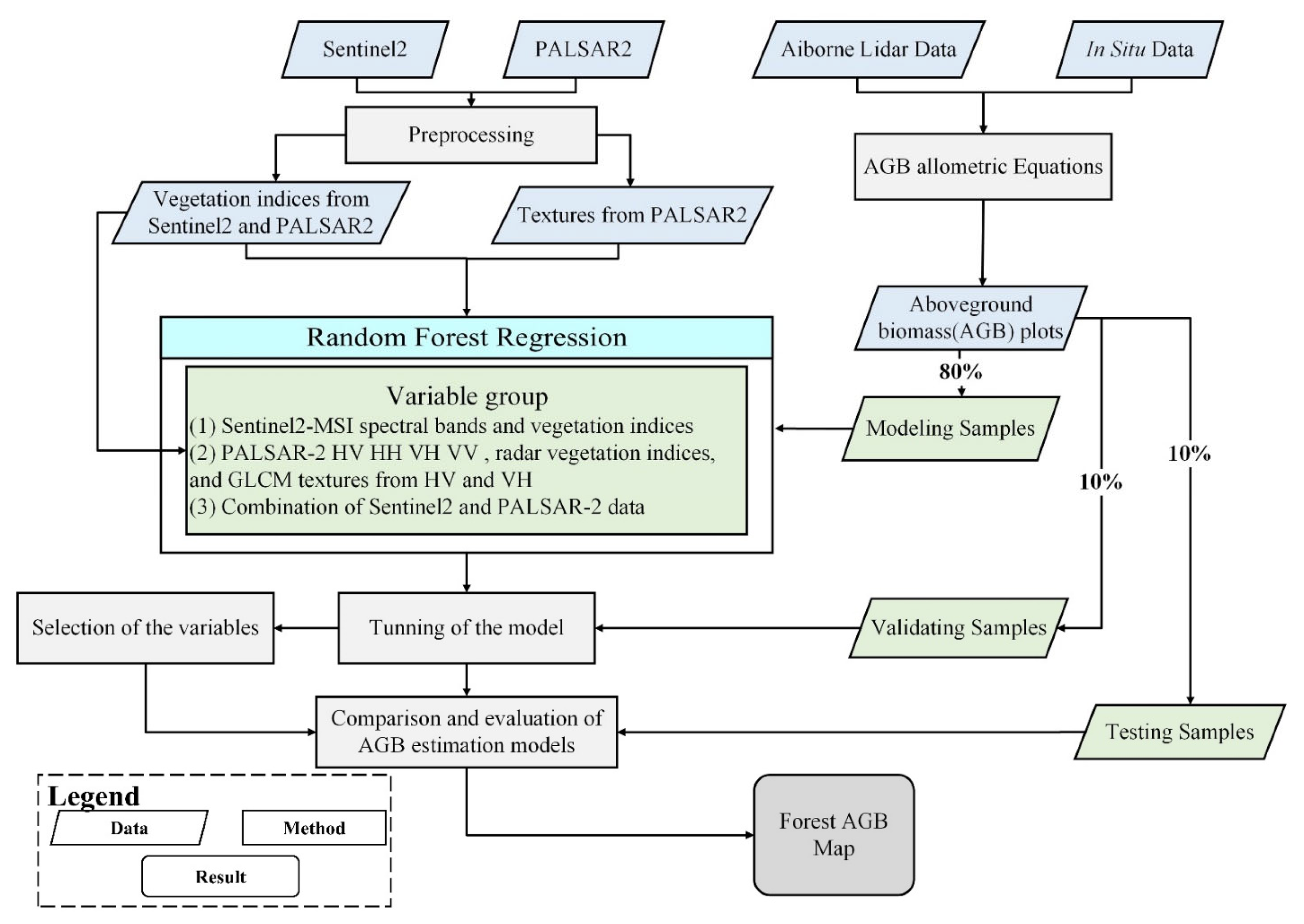
2.2. Data Analysis Process

Figure 2 illustrates the work flow we used for the AGB estimation, which comprises: (1) satellite data collection and preprocessing (resampling, application of a unified coordinate system, filtering, and image clipping); (2) extraction of landscape textures from PALSAR-2 data; (3) computation of indices derived from the satellite images (e.g., the HV and HH polarization ratios; vegetation indices such as NDVI, EVI); (4) model development (selection of the optimal variables, tuning of the hyperparameters); and (5) mapping and estimation of the AGB of the two species in the targeted cities in Ibaraki Prefecture.

2.3. Forest AGB Observed by Airborne Lidar

Airborne lidar data obtained from the Ibaraki Prefecture government was utilized for training the Random Forest model. Ibaraki Prefectural Government preprocessed the airborne lidar product and generated the stem volume through the following procedures:
(1)
collecting and using 40 human measured points (20 for each forest species), each point covering 0.04 ha, for ground-based calibration to evaluate the accuracy of the airborne lidar data related to stem volume calculation,
(2)
collecting airborne lidar data in northern Ibaraki Prefecture on 31 July 2020,
(3)
determining the values of parameters related to the stem biomass calculation calibrated by ground measured plots (i.e., tree species, tree height, and diameter at breast height [DBH]; Table 1 and
(4)
calculating the stem volume from the tree height and DBH using the conventional allometric equations for these species in Japan [42].
The accuracy of the forest parameters used in stem volume calculation are evaluated by the root mean square error (RMSE) with the 40 fields measured data mentioned above; the accuracy of the parameters is shown in Table 2.
RMSE = 1 N ( Y i Y i ) 2
where N is the number of validation plots collected in the field. Y i refers to the field measured parameters. Y i refers to lidar-based predicted parameters in the corresponding position i. The maps of volume for each of the two forest species were generated in the lidar covered area and then converted into AGB values at a 20-m mesh size using a biomass–volume equation with a biomass expansion factor and the tree volume and density by Equation (2) [43]. AGB values are presented as Mg ha−1. It is important to note that only cedar and cypress were considered in the AGB calculation; this is acceptable because we focused on plantations, which are essentially single-species forests. We obtained 201,854 airborne lidar AGB samples for cedar and 69,374 for cypress and used these data as the modeling samples in our subsequent analysis.
AGB = V × WD × BEF
where V is the volume, WD is wood density and BEF is biomass expansion factor [43].

2.4. Remote Sensing Dacta

2.4.1. Processing of PALSAR-2 Data

The Advanced Land Observing Satellite-2 (ALOS-2) is a follow-on mission from ALOS. ALOS-2 has the Phased Array L-band Synthetic Aperture Radar-2 (PALSAR-2), a microwave sensor that can observe, day and night, under any weather conditions. Here, we obtained the 25-m PALSAR2 L-band global mosaic data from May 2019 from the Japan Aerospace Exploration Agency (JAXA; https://www.eorc.jaxa.jp/ALOS/en/palsar_fnf/data/index.html, accessed on 11 June 2021). JAXA preprocessed the PALSAR-2 data, including geometrical calibration against the AW3D30 digital elevation model after 2019. The original SAR data for Japan used the highly sensitive Beam Quad mode, which provides full polarizations, including HH, HV, VV, and VH. The PALSAR-2 signal can be converted into gamma naught backscattering coefficients by using the following equation:
γ 0 = 10 log 10 ( D N 2 ) C F
where γ0 is the backscattering coefficient (gamma naught), DN is the digital number value of each pixel, and CF is the calibration factor, −83 [44]. Moreover, we applied a LEE speckle filter with a kernel window size of 3 × 3 to smooth the images [45]. Before LEE filtering, the radar images were also averaged using a 3 × 3 pixel mean filter to reduce the effect of speckle and spatial heterogeneity of the forest stands and to alleviate the problem of noise from dark spots [24]. Because the plot boundaries of airborne lidar samples may overlie several pixels, using a 3 × 3 window improved performance compared with the single-pixel extraction method [46].
In addition to correcting for backscatter, we calculated the radar vegetation indices for different polarizations and calculated the texture information for HV and VH using a gray-level co-occurrence matrix (GLCM) with a 3 × 3 window size and with a relative displacement vector (d = 1, θ = 45°). The displacement vector explains the spatial distribution of the level pairs separated by d with direction θ [47]. In AGB estimation, the GLCM-derived texture is considered as a kind of predictor that can improve the accuracy of estimation [48]. The texture information can also enlarge the saturation range between AGB and satellite images [49]. We adopted eight popular texture parameters for the VH and HV polarization: mean, variance, homogeneity, contrast, dissimilarity, entropy, second moment, and correlation. Table 3 summarizes the SAR-derived variables used for modeling.

2.4.2. Processing of Sentinel2-MSI Data

Sentinel2-MSI data collected from the European Space Agency (ESA: https://scihub.copernicus.eu/dhus/, accessed on 11 June 2021) were used as optical satellite variables to drive the Random Forest model. Because the optical satellite sensor is easily affected by clouds owing to the wavelengths it uses, we selected data from days with low cloud cover and as close as possible to the time of the AGB data sample collection. From the remaining data, we acquired L2-A level data that had been preprocessed by the ESA, including atmospheric correction and scene classification to L1-B data. The image was acquired on 8 May 2019. The Sentinel-2 MSI sensor provides multispectral data with a spatial resolution ranging from 10 to 60 m. We excluded the 60-m data in this study. We also averaged the Sentinel2 images using a 3 × 3 pixel mean filter to extract the values. We then computed the vegetation indices from the Sentinel-2 data (Table 4) and used those data for modeling.

2.4.3. Extraction of Satellite Images Values from Forest AGB Plots

The AGB plots and satellite images were first unified into the Universal Transverse Mercator (UTM) coordinate system (zone 54 N), with datum of WGS84. Then all of the satellite images were resampled in 20 m resolution using bilinear convolution to meet the resolution of airborne Lidar metric. The geometric center of every airborne Lidar plot was represented as the position of the AGB and extracted the corresponding values of all predictors from the satellite images. Finally, a total of 48 predictors were utilized in a regression model for our analysis: 10 Sentinel-2 MSI spectral bands, 9 Sentinel-2 MSI–derived vegetation indices, 4 ALOS-PALSAR-2 radar backscatter coefficient bands, 16 texture information variables (8 textures each for VH and HV respectively), and 9 radar backscatter coefficient-derived indices.

2.5. Random Forest Regression

Modeling datasets were randomly split into 80%, 10%, and 10% bins for training, validation, and testing samples, respectively, using the train_test_split function in the sklearn package for the Python language.
Random Forest predicts AGB from the remote-sensing predictors by growing many decision trees and averaging every result for each tree. We not only performed inversion modeling for each type of remote sensing data, but also identified (through filtering) the best performing variables for each tree species in this model according to the impurity-based feature importance of the variables, and then we combined the selected variables and used them to process the Random Forest model again. This filtering is necessary because the presence of many redundant variables contributes little to the model, it results in the inclusion of repetitive information, and increases the complexity of the model. For each experiment, we assessed the accuracy of the predictions using the testing data, and then tuned the hyperparameters using the validation data.
Four error statistics were selected to evaluate the model’s performance: the root-mean-square error (RMSE) in Equation (2), the coefficient of determination (R2) in Equation (3), the mean absolute error (MAE) in Equation (4), and the relative RMSE (rRMSE) in Equation (5) as RMSE divided by the mean of the observed AGB values. In the comparison between RMSE and MAE, RMSE is harder to interpret and is more sensitive to outliers than MAE. However, a detailed interpretation is not critical, because variations of the same model will have similar error distributions. Therefore, RMSE is more appropriate as a loss function to tune the hyperparameters for the model as in our case [64]. However, it is still necessary to use MAE together with RMSE to evaluate the variation of model errors [65]. Overall, lower values of RMSE, rRMSE, and MAE and higher R2 indicate better performance of a model. In addition, the smaller the difference between RMSE and MAE, the smaller the variance between errors will be.
R M S E = 1 N ( Y i Y i ) 2
R 2 = 1 i = 1 N ( Y i Y i ) 2 i = 1 N ( Y i Y ¯ ) 2
M A E = 1 N i = 1 N | Y i Y i |
r R M S E = R M S E Y ¯
where N is the number of observed values, Y i is the observed AGB value for observation i, Y i is the predicted AGB value, and Y ¯ is the mean of the observed AGB values. Even though many variables have potential value for estimating AGB, not all are available to be used in the modeling owing to high inter-variable correlation or weak relationships with AGB [66]. Including such variables provides little improvement of accuracy, although it may increase model flexibility. To eliminate the least useful variables, we used the impurity-based feature importance for each variable: the higher the impurity, the more critical the feature. We computed the importance of a feature as the (normalized) total reduction of the criterion; here, we used the mean squared error (MSE) as the criterion brought by that feature, which is also known as the Gini importance.

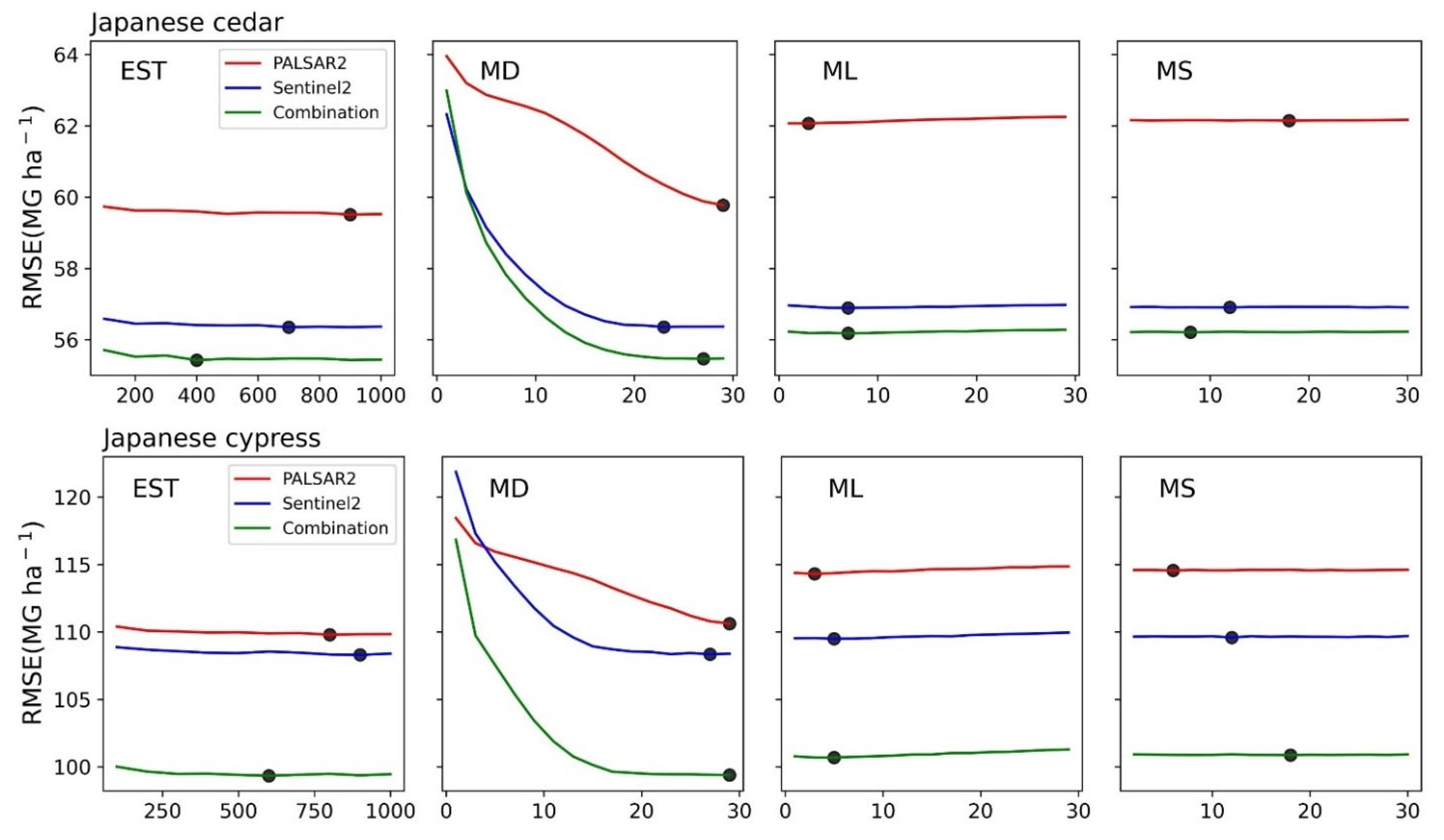
2.6. Determination of the Saturation Level

The saturation level for an individual tree species is crucial for evaluating the estimation result. We defined the AGB saturation level as occurring where a clear pattern of AGB leveling was found in the logarithmic regression slope in a plot of the HV backscatter coefficient against AGB since longer wavelength L-bands with HV backscatter are identified as the most sensitive polarizations to AGB [67]. This approach has been used in previous studies to reveal the relationship between AGB and satellite images and the model’s performance [68,69,70]. Since we used a large sample size in our study, it is difficult to accurately determine the location of the saturation point. Therefore, we adopted an interval sampling method in which we counted the average value of the data points in bins equal to 5 Mg ha−1 in size as the AGB, and removed points with a value greater than 250 Mg ha−1 from the calculation range. Such a kind of approach was accessed in previous research with a huge number of AGB samples [49,71]. Finally, we estimated the saturation levels for each species by examining the slope within every interval (in units of 5 Mg ha−1) with the HV backscatter coefficient. Saturation points in the scatterplot were defined as the points where the slope of each AGB interval was less than 0.1 or where it starts to change in a very disorderly way.

2.7. Evaluation of Forest Resources

After running the models, the best performance model with the highest accuracy was utilized to map the AGB of Japanese cedar and cypress in several target cities with a large area of plantations of the two forest species. The identification of forest area is very crucial for AGB mapping, because mismatched forest distribution maps will cause large estimation errors derived from mismatched estimation models and wrong corresponding forest area. The forest distribution map from the Ibaraki Prefecture government was selected to classify the tree species distribution in our study so that an accurate AGB map could be generated that followed the same standard as the Ibaraki Prefecture AGB map [72]. Finally, we compared the satellite-based AGB map with the forest registered map from Ibaraki Prefecture to evaluate the AGB in the targeted cities.

3. Results

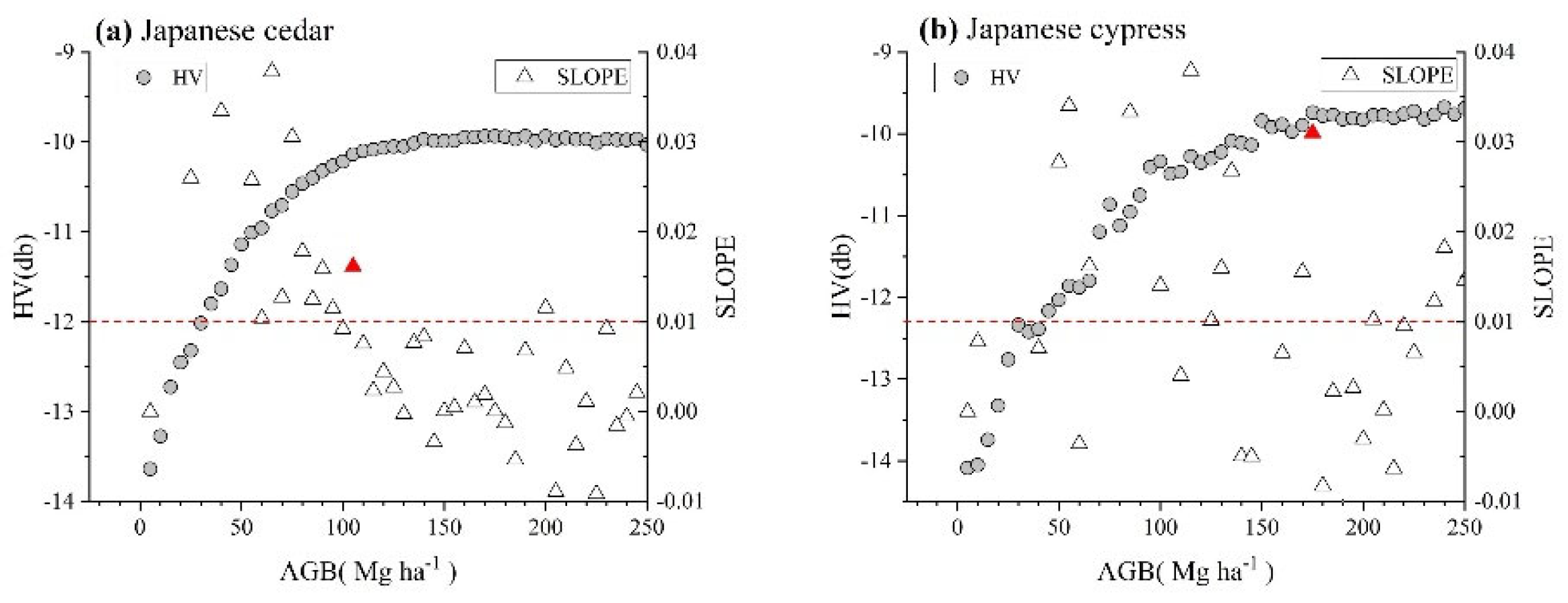
3.1. Determination of the AGB Saturation Level

Figure 3 shows the relationship between the HV backscattering coefficient and AGB. AGB leveled off at a slope of 0.01 dB for the cedar, which represented an AGB of 105 Mg ha−1. However, it was difficult to determine the saturation point for cypress by this method since the slope showed high variation. We defined the saturation point at 175 Mg ha−1, since the HV values leveled off at this point. Nevertheless, when the AGB reached 235 Mg ha−1, the slope continued to increase. The cause of this pattern is unclear; it may have resulted from a relatively small number of samples at high AGB, and the uncertainty of the AGB accuracy rise.

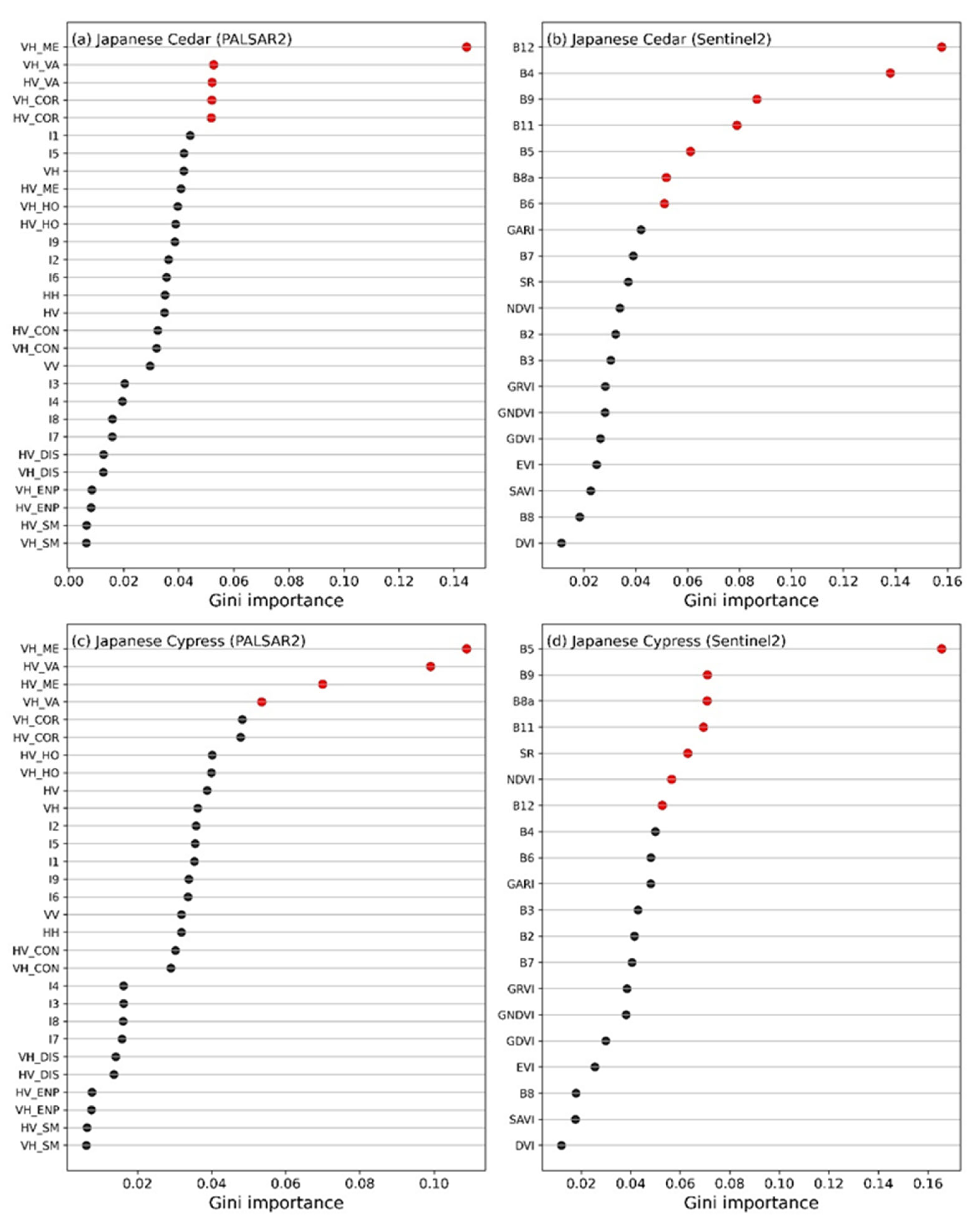
3.2. Development of the Random Forest Model

In the Random Forest model, the importance measures for the variables are affected by the number of variable categories and the measurement scale of the predictor variables [73]. Determining the optimal feature space is an important step for model development. Increasing the number of variables might lead to a high time requirement for the calculations despite a low increase of accuracy [74]. Consequently, we divided the variables into two parts (the PALSAR-2 group and the SENTINEL2-MSI group) and selected the optimal variables on the basis of their importance values. We selected the variables whose importance was greater than 0.05 to interact together and assessed the model again. Figure 4 shows the importance results. The most important variables for cypress (i.e., the variables with a Gini importance greater than 0.05) were VH mean, VH variance, HV variance, VH correlation, and HV correlation (Figure 4a), and Band 5, Band 9, Band 8a, Band 11, SR, NDVI, and Band 12 (Figure 4b). The most important variables for cedar were VH mean, VH variance, HV mean, and HV variance (Figure 4c) and Band 12, Band 4, Band 9, Band 11, Band 5, Band 8a, and Band 6 (Figure 4d).
Random Forest algorithm was run repeatedly to obtain the optimal hyperparameters in each PALSAR-2-based model, each Sentinel2-MSI-based model, and the model that combined the two datasets. We chose four input hyperparameters to determine their optimal values in each model: the number of trees in the forest (EST), the maximum depth of the decision tree (MD), the minimum number of samples (MS) required to split in every internal node, and the minimum number of samples required to be at every leaf node (ML). We reserved 10% of the samples for use as the validation samples to determine their values from the RMSE score. Owing to the size of our dataset, we didn’t perform cross-validation using the validation datasets. We set the number of variables fed to each predictor tree (named max_features in the sklearn package) to the square root of the number of input variables in every model [74], and when we optimized one hyperparameter, we set the others to their default value as MD = 10, ML = 1, MS = 2, and EST = 200. We optimized EST with the determined values of the other three hyperparameters in the last step. The lowest RMSE for the EST tuning indicated the best scores with the optimized hyperparameters. Figure 5 shows the results of the hyperparameter tuning. In every case, the combined model had the best performance. Therefore, we used it to estimate AGB in our subsequent analyses.

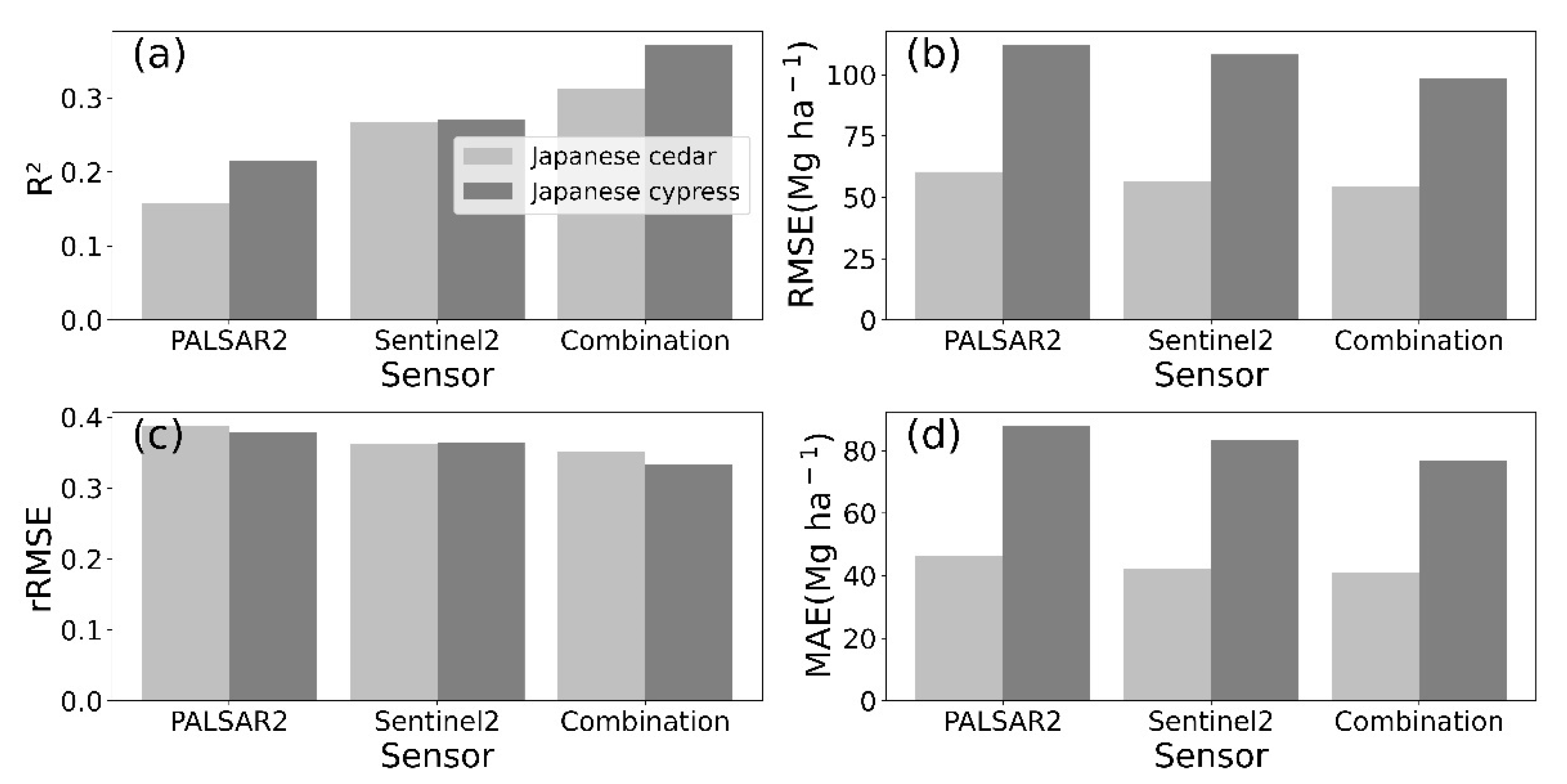
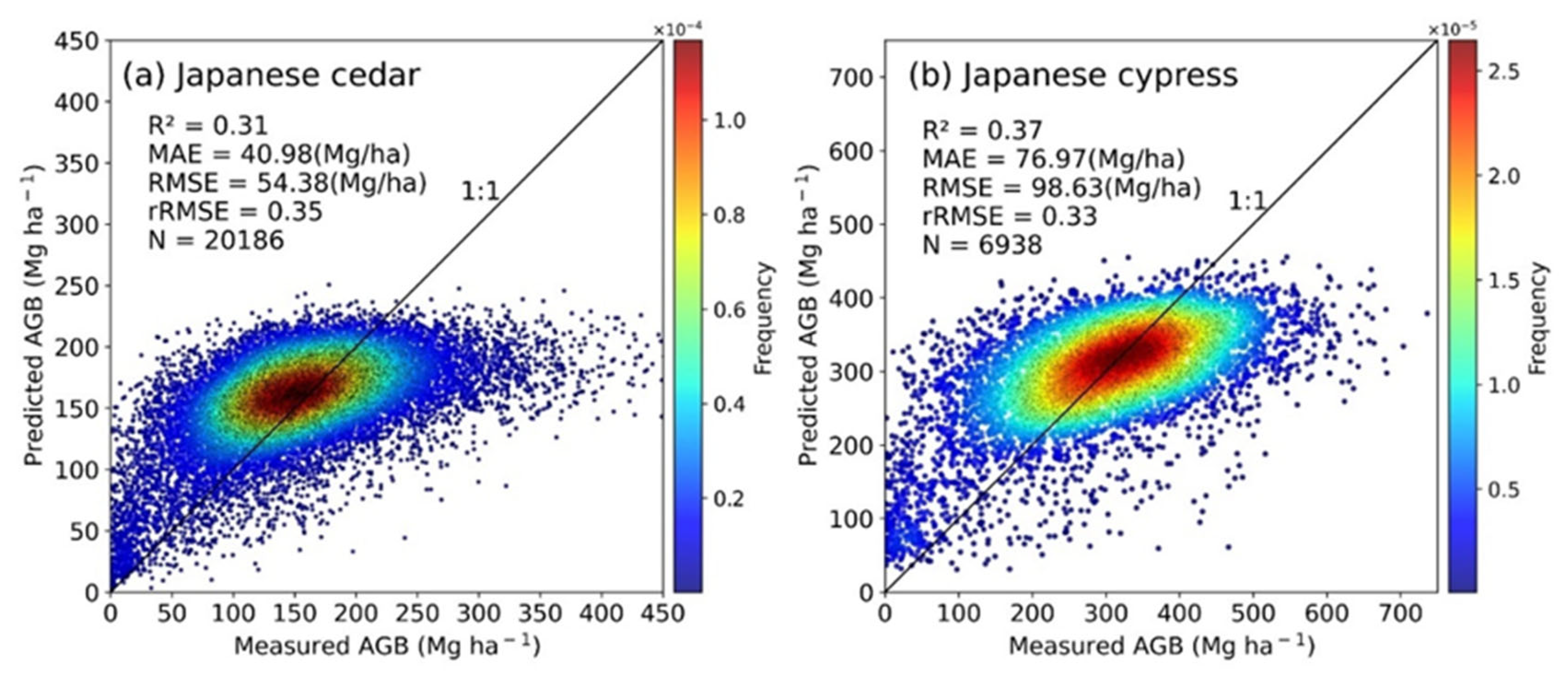
3.3. Model Accuracy Assessment
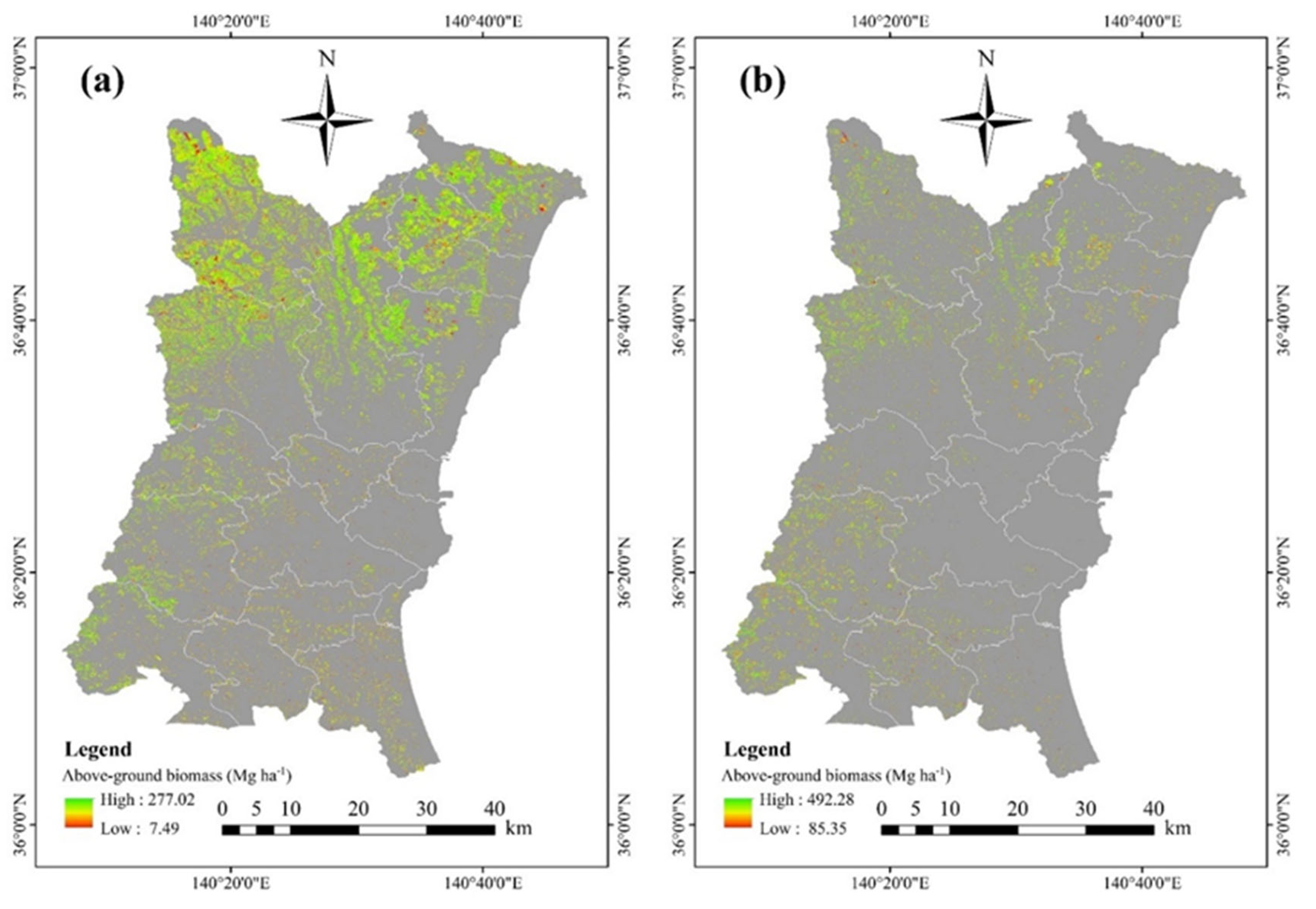
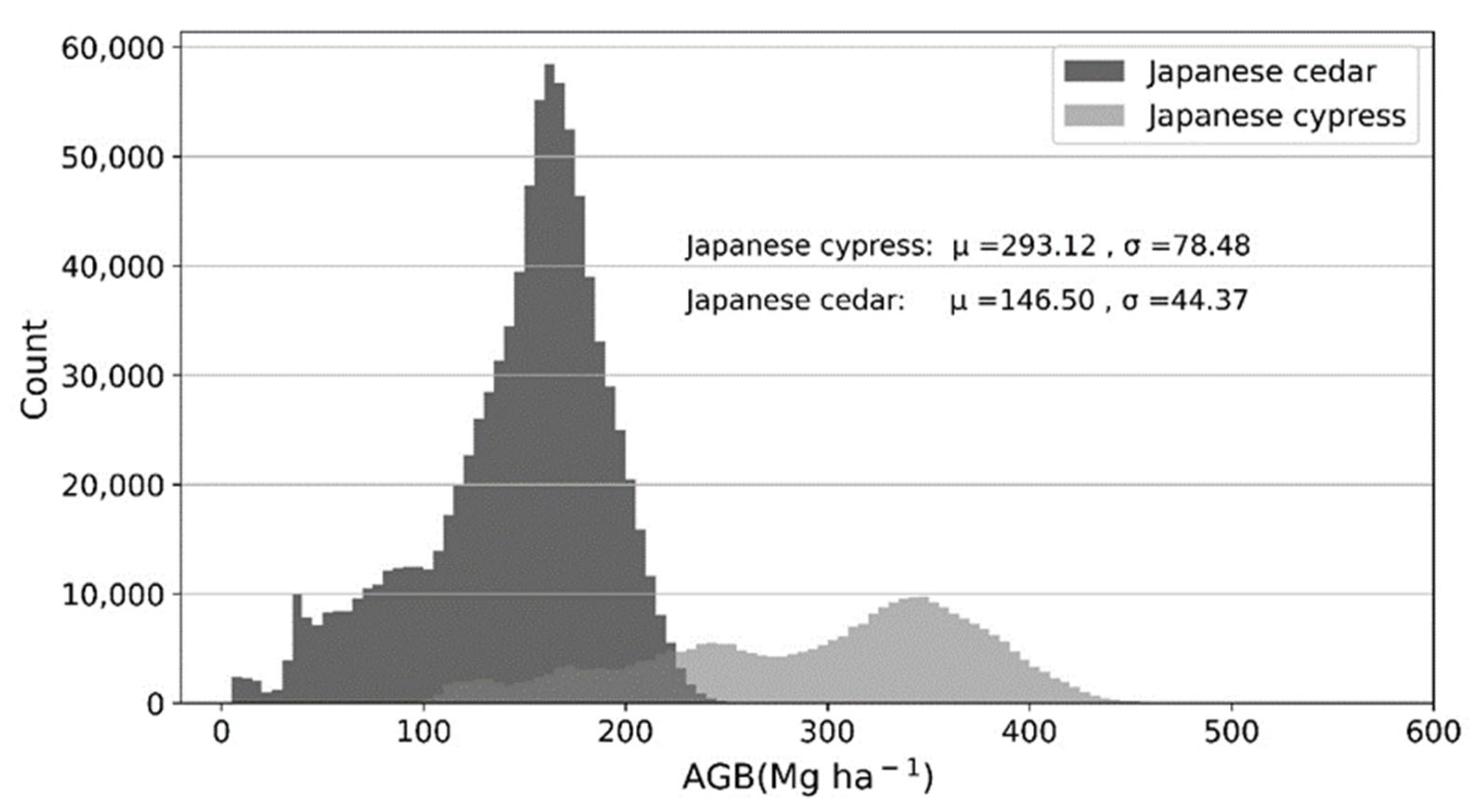
Testing data assessed the model’s accuracy using our selected error statistical indicators. These testing data represented 10% of the overall sample, and excluded data used in model development to keep robustness. For cedar, the Random Forest algorithm was able to predict the AGB with R2 = 0.31, RMSE = 54.38 Mg ha−1, MAE = 40.98 Mg ha−1, and rRMSE = 0.35 from the 20,186 test samples (Figure 6). For cypress, it was able to predict the AGB with R2 = 0.37, RMSE = 98.63 Mg ha−1, MAE = 76.97 Mg ha−1, and rRMSE = 0.33 from the 6938 test samples. For the two tree species, different variables from different remote sensing sensors were important in determining the model’s performance.
Thus, it is necessary to retrieve the relationship between AGB and satellite images by separating for each tree species in the forest.

3.4. Mapping AGB

We generated AGB maps for Japanese cedar and Japanese cypress at 20 m resolution using the Random Forest algorithm for the targeted cities in Ibaraki Prefecture. Appendix A compares the data from the Japanese forestry register record for these cities with the predictions of our model. The AGB ranged from 7.49 to 277.02 Mg ha−1, for Japanese cedar and 85.35 to 492.28 Mg ha−1 for Japanese cypress in the targeted cities (Figure 7).
Japanese cedar and cypress are the main tree species in Japan. Both are evergreen coniferous trees native to Japan. In the overall statistics we analyzed, cypress had a higher AGB than cedar. In terms of the point where AGB saturation occurred according to the HV backscatter coefficient, cypress had a wider range of AGB values than cedar. We think this may be caused by differences in the physical structure of the two species: cypress has a higher biomass range and a larger DBH, which may have led to greater volume scattering, resulting in fluctuations in the relationship between the backscatter coefficient and AGB. Cypress had a much higher mean average AGB (293.12 Mg ha−1) than cedar (146.50 Mg ha−1). However, cedar had a lower standard deviation (44.37 Mg ha−1), with its AGB distributed mainly between 100 and 200 Mg ha−1, whereas Japanese cypress had an AGB distribution with two peaks between 200 and 400 Mg ha−1, with a higher standard deviation (78.48 Mg ha−1). In some previous research, AGB estimation based on the stratification of vegetation types greatly improved the performance [75,76]. We assessed the AGB estimation for two tree species, and found a significant difference in the AGB value distribution (Figure 8). However, the development of an AGB estimation model based on stratification of multiple tree species is more difficult because it requires additional data: (1) vegetation distribution maps for the targeted species, (2) ground-based AGB values classified by species, and (3) a sufficiently large sample size to build a robust model while still leaving data for testing and validation.

4. Discussion

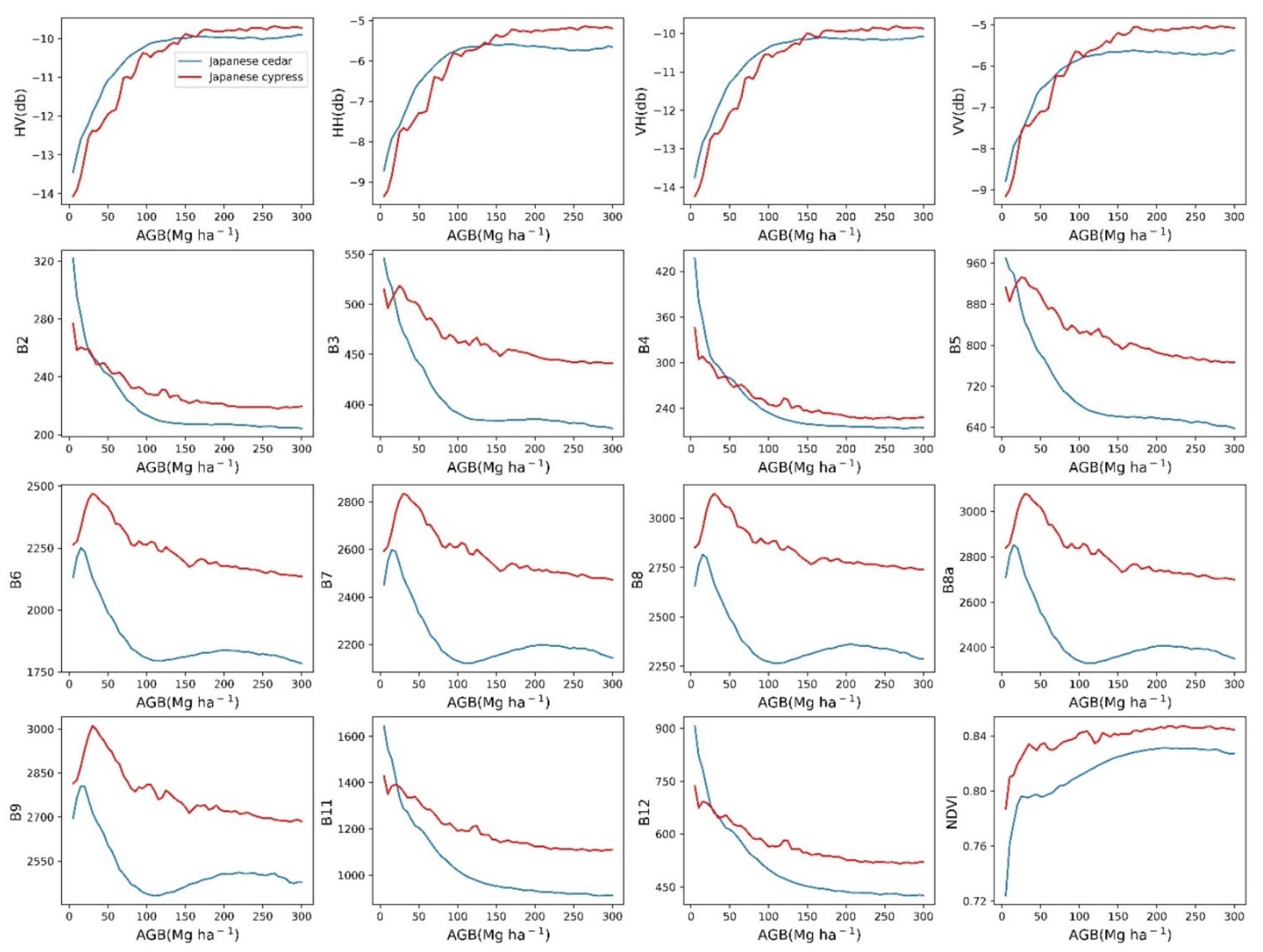
4.1. Role and Limitation of Satellite-Derived Variables in Accurate Estimation of Japanese Cedar and Japanese Cypress AGB

SAR and optical remote sensing have different drawbacks and advantages for AGB estimation. Either dataset by itself is not enough to accurately estimate forest AGB [77]. SAR is relatively unaffected by weather, since it can penetrate clouds and work all day and night. It can also penetrate through the canopy, soil, and dry snow. However, even L-band SAR becomes saturated at an AGB of 100 Mg ha−1 in complex heterogeneous tropical forest structures. In forests with a simple structure and few dominant species, the saturation level could increase to about 250 Mg ha−1 [78]. We found that the optical data were more resistant than the SAR data to AGB saturation for Japanese cedar and cypress at high AGB values (Figure 9).
To identify the saturation level for the two tree species, we used the HV backscatter from the SAR data. Cedar became saturated at 105 Mg ha−1 and cypress at 175 Mg ha−1. Even though these species are similar in their structure and living conditions, they showed a clear difference in the saturation level with SAR at relatively low values. In contrast, the optical sensors are strongly affected by weather conditions, but also show AGB saturation. Because these different sensor data have different advantages and drawbacks, integration of radar data with optical-sensor data has the potential to improve AGB estimation because it may reduce the number of mixed pixels and data saturation problems [66].
Our aim was to develop models of cedar and cypress for estimating AGB from two types of satellite data: L-band microwave radar data from PALSAR-2 and multispectral optical remote sensing data from Sentinel2-MSI. For our study species, microwave remote sensing was more sensitive to saturation than optical remote sensing. Therefore, the estimation results of the PALSAR-2 model performed worse in both species (Figure 10). In contrast, the model that combined the two datasets performed best in every case. This demonstrates that combining different types of remote sensing data can improve the estimation accuracy and AGB range.
However, underestimation at high AGB values remains large, since satellite information (especially microwave and optical remote sensing data) inevitably became saturated. Although this problem can be alleviated by adding texture information [49] or by combining multi-source remote sensing data, as we did in this study, it is still fundamentally difficult to solve the saturation problem. The airborne lidar data have a high range for estimation of AGB (i.e., high resistance to saturation) owing to their wavelength characteristics, but such data are expensive, which makes it impossible to cover large areas such as a whole country or continent, unlike the space satellite data that are used for large-area studies. Hence, airborne lidar data have mainly been used in small areas [79]. Establishing a model that would extend AGB estimation to large areas by combining data from field plots, airborne lidar, and space satellite data thus has considerable potential to enlarge the area that could be surveyed with airborne lidar data [80]. In such a method, lidar data and satellite remote sensing data could be combined to support large-area AGB predictions, but more tests are still needed, and the analytical framework must be improved to support this use of multisource data. This is because the use of different buffer sizes to combine data from different sources can decrease the accuracy of AGB estimation [80].
The Random Forest model has an excellent predictive ability but has the characteristics of tree-regression. The algorithm operates by constructing many decision trees during training and outputs the predicted mean or mode of the individual decision trees. The AGB prediction averages all variables extracted from the satellite images. However, the algorithm cannot predict the value from the training samples. Using only the satellite-based data, the problem becomes more severe, since saturation occurred in all of the satellite data. Because our approach overlays the underestimation of high AGB values with AGB saturation in the satellite images, it is hard to obtain good performance in forests with high AGB.

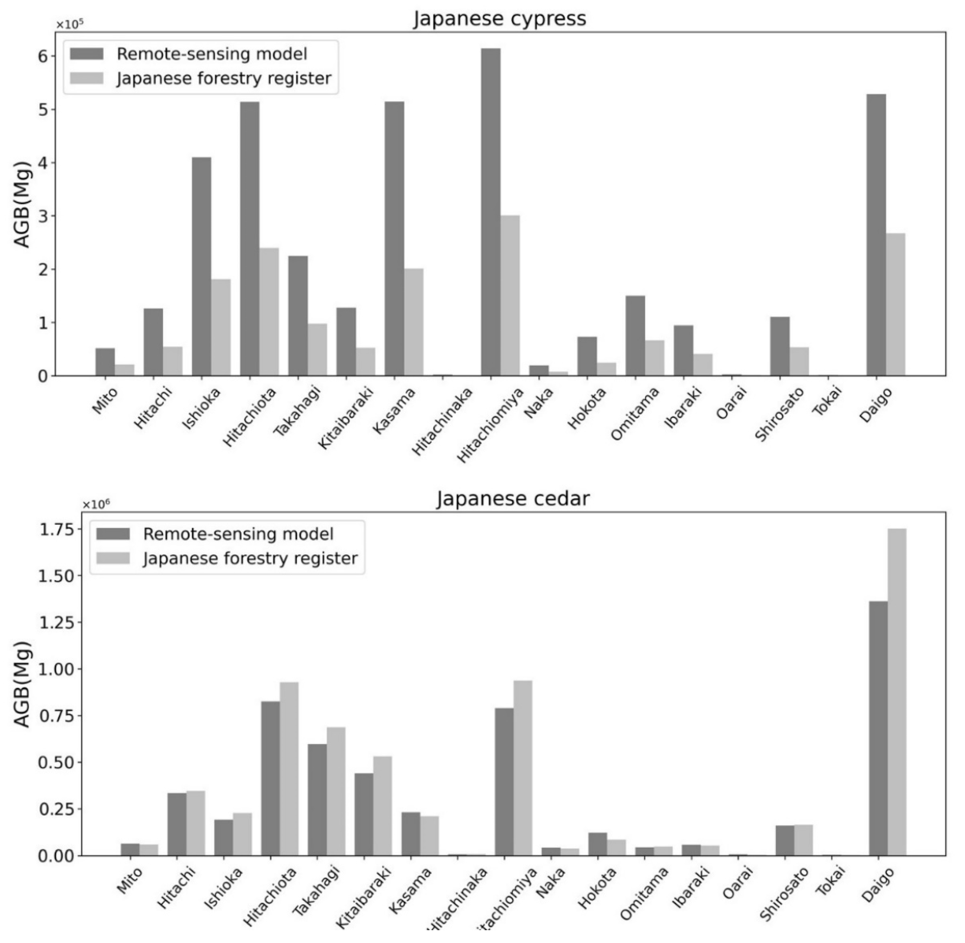
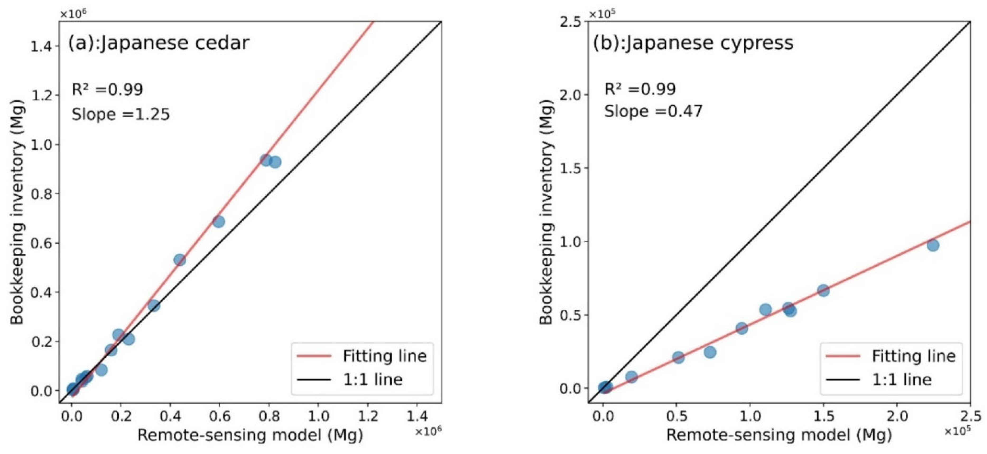
4.2. Benchmark AGB Estimated in the Japanese Forest Inventory

The satellite-derived AGB map was compared with government statistics for the total AGB in every targeted city (Figure 11). The forestry statistics in Japan are based on the forest register, which is used for forest management. Japanese forests are managed as land units called sub-compartments. The forest register records forest conditions for every sub-compartment, such as its area, tree species, mean age, and stand volume. Japanese law requires that the forest register be updated every 5 years. The satellite-derived AGB was more significant than the value in the register in Ibaraki, and some previous studies also concluded that the forest register underestimated the forest volume [81]. Japan’s Forestry and Forest Products Research Institute compared the register’s data with a field measurement at 10,189 sub-compartments throughout Japan, and found that the field-measured forest volume was 1.88 times the value in the forest register for Japan as a whole [82]. These results agree with the present results for cypress, since the estimated AGB was larger than the value in the register. A previous study analyzed airborne lidar data for all of Ehime Prefecture (a prefecture located in southwestern Japan), and found that the total forest volume in Ehime was 2.01 times the value in the register [83]. The authors mentioned that errors in both the lidar estimates and the register contributed to this difference, but suggested that the errors in the register were much larger. These previous studies suggest that our results are reasonable, and the satellite estimates are closer than the register to the actual values. The forest register may underestimate the forest volume for at least two reasons: (1) it records only an estimated value based on the tree species and forest age, not a field-measured value, and (2) the empirical yield tables (used for the estimation that produces the register values) were developed in the 1950s and 1960s and have not been updated since then, so their gap relative to the actual values may have increased [82,84]. One reason for this gap is that there were insufficient measurement data for old-growth forests to support empirical development of yield tables, so the tables underestimate the volume of old-growth forests. Accurate forest resource information is fundamental for forest management, and the forest register, which does not have a monitoring function for actual forests, cannot provide the necessary support. Our approach may solve this problem.

4.3. Uncertainty in AGB Estimation

The geographic location between the airborne lidar sample points and satellite pixels will bring significant uncertainty. We use the geometric center of an airborne Lidar sample point with a resolution of 20 m (0.04 hectares) to extract satellite pixel values. Nevertheless, an area of 0.04 hectares cannot cover a plurality of pixels well, leading to missing and biased parts of the data. Although we have alleviated the uncertainty mentioned above through the mean filter, using the mean filter will cause some irrelevant pixels to be calculated into the target pixels, especially when some different tree species are inlaid with each other or in the boundary of the forest area [85]. One method is to select only a cluster of airborne radar sample points gathered by a single tree species as the ground data points and calculate the average value of the pixel points covered by the sample points as the satellite data value corresponding to the airborne lidar plot, but this would significantly increase the complexity of the calculation.
The temporal difference between airborne Lidar and satellite images can also be uncertain. As cloud cover often occurs in the northern part of our research area, in order to avoid the impact of this situation on detection, it is challenging to select satellite data that is the same as or very close to the ground sample point collection time and dozens of days may lead to a difference of forest growth which may lead to temporal variability in satellite images [86]. The change of the period has led to errors in the agreement between the biomass and satellite data. One of the methods focuses on the growth period, ignoring the influence of the year, and selecting ground sample points in other years to collect the satellite data of the corresponding month, but this may lead to forest changes caused by excessive time. Therefore, it is essential to check the forest to see massive changes due to people’s affection or natural hazards.
Finally, there is the error caused by the biomass equation because we used the airborne lidar data as the “real” sample data and satellite data for correction. This method provides more sample data than traditional human measurement sample points. A more extensive sample set will avoid the curse of dimensionality caused by too many satellite variables and has better robustness compared to small data set. However, the method of calculating the stock volume by obtaining the parameter values of the trees and converting it through the volume-biomass transferring equation will also have a significant deviation compared with the actual biomass calculation equation of a single tree called recording and grouping errors [79]. However, AGB estimations using only field data over large areas suffer an enormous error rate. Therefore, choosing a large amount of data or a small amount of data with higher accuracy needs to be traded off carefully.

5. Conclusions

We developed robust and effective models to estimate the AGB of Japanese cedar and cypress by a machine learning approach. As far as we know, no other studies have used remote sensing data to retrieve the AGB of those two types of forest at prefecture level. We hope to create a new approach to remedying the lack of forest biomass in Japan. By combining PALSAR-2 and Sentinel2-MSI data and using a large number of validation samples from lidar-based AGB plots, we increased the accuracy of AGB prediction for both species compared with using only one data source. The hyperparameter tuning in Random Forest also improved estimation accuracy, especially for the depth of the tree structure. Because the choice of modeling variables strongly affects the accuracy and simplicity of the models, our approach also helps to select the optimal variables for inclusion in the final model. The texture information for the PALSAR-2 images played an important role in estimating AGB, and this confirms the value of retaining SAR texture information.
Although our method provided a scientific basis for more accurately estimating AGB of the two tree species in our study, more work will be necessary to adapt the method to multi-species forests. The methodology could then be adopted for mapping and estimating forest biomass in Japan and updating the forest register. This use of remote sensing will provide a cost-efficient way to estimate forest conditions and their spatial and temporal variation.

Author Contributions

Conceptualization, T.K. and M.H.; methodology, T.K. and M.H.; software, H.L.; validation, T.K. and M.H.; formal analysis, H.L., T.K. and L.W.; investigation, H.L.; resources, T.K. and M.H.; data curation, H.L. and M.H.; writing—original draft preparation, H.L.; writing—review and editing, T.K. and M.H.; visualization, H.L.; supervision, T.K.; project administration, T.K.; funding acquisition, T.K. All authors have read and agreed to the published version of the manuscript.

Funding

This research was funded by the Telecommunications Advancement Foundation.

Institutional Review Board Statement

Not applicable.

Informed Consent Statement

Not applicable.

Data Availability Statement

Not applicable.

Acknowledgments

This study was supported by JAXA Research Announcement on Earth Observations (No. ER2A2N208). The airborne lidar data was provided by the Ibaraki Prefectural Government (permit No. RINSEI-264).

Conflicts of Interest

The authors declare no conflict of interest.

Appendix A

Figure A1 compares the data in the Japanese forestry register with predictions from the remote-sensing model for the targeted cities in Ibaraki Prefecture.
Figure A1. The aboveground biomass (AGB) estimated by the remote-sensing model and recorded in the Japanese forestry register for Japanese cedar and Japanese cypress in the 17 targeted cities in Ibaraki Prefecture.
Remotesensing 14 00468 g0a1

References

  1. Dong, J.; Kaufmann, R.K.; Myneni, R.B.; Tucker, C.J.; Kauppi, P.E.; Liski, J.; Buermann, W.; Alexeyev, V.; Hughes, M.K. Remote sensing estimates of boreal and temperate forest woody biomass: Carbon pools, sources, and sinks. Remote Sens. Environ. 2003, 84, 393–410. [Google Scholar] [CrossRef] [Green Version]
  2. Gower, S.T. Patterns and Mechanisms of The Forest Carbon Cycle. Annu. Rev. Environ. Resour. 2003, 28, 169–204. [Google Scholar] [CrossRef]
  3. Fahey, T.J.; Woodbury, P.B.; Battles, J.J.; Goodale, C.L.; Hamburg, S.P.; Ollinger, S.V.; Woodall, C.W. Forest carbon storage: Ecology, management, and policy. Front. Ecol. Environ. 2010, 8, 245–252. [Google Scholar] [CrossRef] [Green Version]
  4. Goetz, S.; Dubayah, R. Advances in remote sensing technology and implications for measuring and monitoring forest carbon stocks and change. Carbon Manag. 2014, 2, 231–244. [Google Scholar] [CrossRef]
  5. Chojnacky, D.C.; Heath, L.S.; Jenkins, J.C. Updated generalized biomass equations for North American tree species. Forestry 2013, 87, 129–151. [Google Scholar] [CrossRef] [Green Version]
  6. Kuenzer, C.; Bluemel, A.; Gebhardt, S.; Quoc, T.V.; Dech, S. Remote Sensing of Mangrove Ecosystems: A Review. Remote Sens. 2011, 3, 878–928. [Google Scholar] [CrossRef] [Green Version]
  7. Zolkos, S.G.; Goetz, S.J.; Dubayah, R. A meta-analysis of terrestrial aboveground biomass estimation using lidar remote sensing. Remote Sens. Environ. 2013, 128, 289–298. [Google Scholar] [CrossRef]
  8. Lefsky, M.A. A global forest canopy height map from the Moderate Resolution Imaging Spectroradiometer and the Geoscience Laser Altimeter System. Geophys. Res. Lett. 2010, 37. [Google Scholar] [CrossRef] [Green Version]
  9. Ioki, K.; Tsuyuki, S.; Hirata, Y.; Phua, M.-H.; Wong, W.V.C.; Ling, Z.-Y.; Saito, H.; Takao, G. Estimating above-ground biomass of tropical rainforest of different degradation levels in Northern Borneo using airborne LiDAR. For. Ecol. Manag. 2014, 328, 335–341. [Google Scholar] [CrossRef]
  10. Jubanski, J.; Ballhorn, U.; Kronseder, K.; Siegert, F. Detection of large above-ground biomass variability in lowland forest ecosystems by airborne LiDAR. Biogeosciences 2013, 10, 3917–3930. [Google Scholar] [CrossRef] [Green Version]
  11. Réjou-Méchain, M.; Tymen, B.; Blanc, L.; Fauset, S.; Feldpausch, T.R.; Monteagudo, A.; Phillips, O.L.; Richard, H.; Chave, J. Using repeated small-footprint LiDAR acquisitions to infer spatial and temporal variations of a high-biomass Neotropical forest. Remote Sens. Environ. 2015, 169, 93–101. [Google Scholar] [CrossRef]
  12. Popescu, S.C. Estimating biomass of individual pine trees using airborne lidar. Biomass Bioenergy 2007, 31, 646–655. [Google Scholar] [CrossRef]
  13. Wang, H.; Seaborn, T.; Wang, Z.; Caudill, C.C.; Link, T.E. Modeling tree canopy height using machine learning over mixed vegetation landscapes. Int. J. Appl. Earth Obs. Geoinf. 2021, 101, 102353. [Google Scholar] [CrossRef]
  14. Nguyen, T.H.; Jones, S.; Soto-Berelov, M.; Haywood, A.; Hislop, S. Landsat Time-Series for Estimating Forest Aboveground Biomass and Its Dynamics across Space and Time: A Review. Remote Sens. 2019, 12, 98. [Google Scholar] [CrossRef] [Green Version]
  15. Chauhan, S.; Darvishzadeh, R.; Boschetti, M.; Nelson, A. Estimation of crop angle of inclination for lodged wheat using multi-sensor SAR data. Remote Sens. Environ. 2020, 236, 111488. [Google Scholar] [CrossRef]
  16. Le Hegarat-Mascle, S.; Zribi, M.; Alem, F.; Weisse, A.; Loumagne, C. Soil moisture estimation from ERS/SAR data: Toward an operational methodology. IEEE Trans. Geosci. Remote Sens. 2002, 40, 2647–2658. [Google Scholar] [CrossRef]
  17. Neumann, M.; Ferro-Famil, L.; Reigber, A. Estimation of Forest Structure, Ground, and Canopy Layer Characteristics from Multibaseline Polarimetric Interferometric SAR Data. IEEE Trans. Geosci. Remote Sens. 2010, 48, 1086–1104. [Google Scholar] [CrossRef] [Green Version]
  18. Fagan, M.; DeFries, R. Measurement and Monitoring of the World’s Forests: A Review and Summary of Remote Sensing Technical Capability, 2009–2015; Resources of the Future: Washington, DC, USA, 2009; 131p. [Google Scholar]
  19. Imhoff, M.L. Radar backscatter and biomass saturation: Ramifications for global biomass inventory. IEEE Trans. Geosci. Remote Sens. 1995, 33, 511–518. [Google Scholar] [CrossRef]
  20. Amini, J.; Sumantyo, J.T.S. Employing a Method on SAR and Optical Images for Forest Biomass Estimation. IEEE Trans. Geosci. Remote Sens. 2009, 47, 4020–4026. [Google Scholar] [CrossRef]
  21. Lillesand, T.; Kiefer, R.W.; Chipman, J. Remote Sensing and Image Interpretation; John Wiley & Sons: Hoboken, NJ, USA, 2015. [Google Scholar]
  22. Pflugmacher, D.; Cohen, W.B.; Kennedy, R.E. Using Landsat-derived disturbance history (1972–2010) to predict current forest structure. Remote. Sens. Environ. 2012, 122, 146–165. [Google Scholar] [CrossRef]
  23. Carreiras, J.M.B.; Vasconcelos, M.J.; Lucas, R.M. Understanding the relationship between aboveground biomass and ALOS PALSAR data in the forests of Guinea-Bissau (West Africa). Remote Sens. Environ. 2012, 121, 426–442. [Google Scholar] [CrossRef]
  24. Peregon, A.; Yamagata, Y. The use of ALOS/PALSAR backscatter to estimate above-ground forest biomass: A case study in Western Siberia. Remote Sens. Environ. 2013, 137, 139–146. [Google Scholar] [CrossRef]
  25. Lucas, R.; Armston, J.; Fairfax, R.; Fensham, R.; Accad, A.; Carreiras, J.; Kelley, J.; Bunting, P.; Clewley, D.; Bray, S.; et al. An Evaluation of the ALOS PALSAR L-Band Backscatter—Above Ground Biomass Relationship Queensland, Australia: Impacts of Surface Moisture Condition and Vegetation Structure. IEEE J. Sel. Top. Appl. Earth Obs. Remote Sens. 2010, 3, 576–593. [Google Scholar] [CrossRef]
  26. Cartus, O.; Santoro, M.; Kellndorfer, J. Mapping Forest aboveground biomass in the Northeastern United States with ALOS PALSAR dual-polarization L-band. Remote Sens. Environ. 2012, 124, 466–478. [Google Scholar] [CrossRef]
  27. Forkuor, G.; Benewinde Zoungrana, J.-B.; Dimobe, K.; Ouattara, B.; Vadrevu, K.P.; Tondoh, J.E. Above-ground biomass mapping in West African dryland forest using Sentinel-1 and 2 datasets—A case study. Remote Sens. Environ. 2020, 236, e111496. [Google Scholar] [CrossRef]
  28. Dang, A.T.N.; Nandy, S.; Srinet, R.; Luong, N.V.; Ghosh, S.; Senthil Kumar, A. Forest aboveground biomass estimation using machine learning regression algorithm in Yok Don National Park, Vietnam. Ecol. Inform. 2019, 50, 24–32. [Google Scholar] [CrossRef]
  29. Breiman, L. Random forests. Mach. Learn. 2001, 45, 5–32. [Google Scholar] [CrossRef] [Green Version]
  30. Rodríguez-Veiga, P.; Quegan, S.; Carreiras, J.; Persson, H.J.; Fransson, J.E.S.; Hoscilo, A.; Ziółkowski, D.; Stereńczak, K.; Lohberger, S.; Stängel, M.; et al. Forest biomass retrieval approaches from earth observation in different biomes. Int. J. Appl. Earth Obs. Geoinf. 2019, 77, 53–68. [Google Scholar] [CrossRef]
  31. Olden, J.D.; Lawler, J.J.; Poff, N.L. Machine learning methods without tears: A primer for ecologists. Q. Rev. Biol. 2008, 83, 171–193. [Google Scholar] [CrossRef] [PubMed] [Green Version]
  32. Ahmed, O.S.; Franklin, S.E.; Wulder, M.A.; White, J.C. Characterizing stand-level forest canopy cover and height using Landsat time series, samples of airborne LiDAR, and the Random Forest algorithm. ISPRS J. Photogramm. Remote Sens. 2015, 101, 89–101. [Google Scholar] [CrossRef]
  33. Wang, Y.; Zhang, X.; Guo, Z. Estimation of tree height and aboveground biomass of coniferous forests in North China using stereo ZY-3, multispectral Sentinel-2, and DEM data. Ecol. Indic. 2021, 126, 107645. [Google Scholar] [CrossRef]
  34. Ye, Q.; Yu, S.; Liu, J.; Zhao, Q.; Zhao, Z. Aboveground biomass estimation of black locust planted forests with aspect variable using machine learning regression algorithms. Ecol. Indic. 2021, 129, 107948. [Google Scholar] [CrossRef]
  35. Avitabile, V.; Herold, M.; Heuvelink, G.B.; Lewis, S.L.; Phillips, O.L.; Asner, G.P.; Armston, J.; Ashton, P.S.; Banin, L.; Bayol, N.; et al. An integrated pan-tropical biomass map using multiple reference datasets. Glob. Change Biol. 2016, 22, 1406–1420. [Google Scholar] [CrossRef] [Green Version]
  36. Houghton, R.A. Aboveground Forest Biomass and the Global Carbon Balance. Glob. Chang. Biol. 2005, 11, 945–958. [Google Scholar] [CrossRef]
  37. Mermoz, S.; Le Toan, T.; Villard, L.; Réjou-Méchain, M.; Seifert-Granzin, J. Biomass assessment in the Cameroon savanna using ALOS PALSAR data. Remote Sens. Environ. 2014, 155, 109–119. [Google Scholar] [CrossRef]
  38. Rodríguez-Veiga, P.; Saatchi, S.; Tansey, K.; Balzter, H. Magnitude, spatial distribution and uncertainty of forest biomass stocks in Mexico. Remote Sens. Environ. 2016, 183, 265–281. [Google Scholar] [CrossRef] [Green Version]
  39. Kellndorfer, J.; Walker, W.; Kirsch, K.; Fiske, G.; Bishop, J.; LaPoint, L.; Hoppus, M.; Westfall, J. NACP Aboveground Biomass and Carbon Baseline Data, V. 2 (NBCD 2000), USA. 2000. Available online: https://daac.ornl.gov/NACP/guides/NBCD_2000_V2.html (accessed on 5 April 2021).
  40. Barbosa, J.M.; Broadbent, E.N.; Bitencourt, M.D. Remote Sensing of Aboveground Biomass in Tropical Secondary Forests: A Review. Int. J. For. Res. 2014, 2014, 715796. [Google Scholar] [CrossRef]
  41. Japan Forestry Agency. Data for Japanese Cedar and Cypress Plantations; Japan Forestry Agency: Tokyo, Japan, 2014. [Google Scholar]
  42. Japan Forestry Agency. Table of Standing Tree Trunk Volume: Western Japan Version; Forestry Survey Group: Tokyo, Japan, 1970. [Google Scholar]
  43. Ministry of the Environment; Center for Global Environmental Research (CGER); National Institute for Environmental Studies (NIES). National Greenhouse Gas Inventory Report of JAPAN; National Institute for Environmental Studies: Onogawa, Japan, 2021. [Google Scholar]
  44. Shimada, M.; Itoh, T.; Motooka, T.; Watanabe, M.; Shiraishi, T.; Thapa, R.; Lucas, R. New global forest/non-forest maps from ALOS PALSAR data (2007–2010). Remote Sens. Environ. 2014, 155, 13–31. [Google Scholar] [CrossRef]
  45. Lee, J.S.; Jurkevich, L.; Dewaele, P.; Wambacq, P.; Oosterlinck, A. Speckle filtering of synthetic aperture radar images: A review. Remote Sens. Rev. 1994, 8, 313–340. [Google Scholar] [CrossRef]
  46. Tian, X.; Su, Z.; Chen, E.; Li, Z.; van der Tol, C.; Guo, J.; He, Q. Estimation of forest above-ground biomass using multi-parameter remote sensing data over a cold and arid area. Int. J. Appl. Earth Obs. Geoinf. 2012, 14, 160–168. [Google Scholar] [CrossRef]
  47. Haralick, R.M.; Shanmugam, K.; Dinstein, I.H. Textural features for image classification. IEEE Trans. Syst. Man Cybern. 1973, 3, 610–621. [Google Scholar] [CrossRef] [Green Version]
  48. Thapa, R.B.; Watanabe, M.; Motohka, T.; Shimada, M. Potential of high-resolution ALOS–PALSAR mosaic texture for aboveground forest carbon tracking in tropical region. Remote Sens. Environ. 2015, 160, 122–133. [Google Scholar] [CrossRef]
  49. Hayashi, M.; Motohka, T.; Sawada, Y. Aboveground Biomass Mapping Using ALOS-2/PALSAR-2 Time-Series Images for Borneo’s Forest. IEEE J. Sel. Top. Appl. Earth Obs. Remote Sens. 2019, 12, 5167–5177. [Google Scholar] [CrossRef]
  50. Avtar, R.; Sawada, H.; Takeuchi, W.; Singh, G. Characterization of forests and deforestation in Cambodia using ALOS/PALSAR observation. Geocarto Int. 2012, 27, 119–137. [Google Scholar] [CrossRef]
  51. Lehmann, E.A.; Caccetta, P.A.; Zhou, Z.-S.; McNeill, S.J.; Wu, X.; Mitchell, A.L. Joint processing of Landsat and ALOS-PALSAR data for forest mapping and monitoring. IEEE Trans. Geosci. Remote Sens. 2011, 50, 55–67. [Google Scholar] [CrossRef]
  52. Huggannavar, V.; Shetty, A. Biomass Estimation Using Synergy of ALOS-PALSAR and Landsat Data in Tropical Forests of Brazil. In Applications of Geomatics in Civil Engineering; Springer: Singapore, 2020. [Google Scholar]
  53. Dong, J.; Xiao, X.; Sheldon, S.; Biradar, C.; Duong, N.D.; Hazarika, M. A comparison of forest cover maps in Mainland Southeast Asia from multiple sources: PALSAR, MERIS, MODIS and FRA. Remote Sens. Environ. 2012, 127, 60–73. [Google Scholar] [CrossRef]
  54. Kim, Y.; Jackson, T.; Bindlish, R.; Lee, H.; Hong, S. Radar vegetation index for estimating the vegetation water content of rice and soybean. IEEE Geosci. Remote Sens. Lett. 2011, 9, 564–568. [Google Scholar]
  55. Rouse, J.W.; Haas, R.H.; Schell, J.A.; Deering, D.W. Monitoring vegetation systems in the Great Plains with ERTS. NASA Spec. Publ. 1974, 351, 309. [Google Scholar]
  56. Huete, A.; Didan, K.; Miura, T.; Rodriguez, E.P.; Gao, X.; Ferreira, L.G. Overview of the radiometric and biophysical performance of the MODIS vegetation indices. Remote Sens. Environ. 2002, 83, 195–213. [Google Scholar] [CrossRef]
  57. Tucker, C.J. Red and photographic infrared linear combinations for monitoring vegetation. Remote Sens. Environ. 1979, 8, 127–150. [Google Scholar] [CrossRef] [Green Version]
  58. Gitelson, A.A.; Kaufman, Y.J.; Merzlyak, M.N. Use of a green channel in remote sensing of global vegetation from EOS-MODIS. Remote Sens. Environ. 1996, 58, 289–298. [Google Scholar] [CrossRef]
  59. Huete, A.R. A soil-adjusted vegetation index (SAVI). Remote Sens. Environ. 1988, 25, 295–309. [Google Scholar] [CrossRef]
  60. Gitelson, A.A.; Merzlyak, M.N. Remote sensing of chlorophyll concentration in higher plant leaves. Adv. Space Res. 1998, 22, 689–692. [Google Scholar] [CrossRef]
  61. Sripada, R.P. Determining in-Season Nitrogen Requirements for Corn Using Aerial Color-Infrared Photography; North Carolina State University: Raleigh, NC, USA, 2005. [Google Scholar]
  62. Birth, G.S.; McVey, G.R. Measuring the color of growing turf with a reflectance spectrophotometer 1. Agron. J. 1968, 60, 640–643. [Google Scholar] [CrossRef]
  63. Sripada, R.P.; Heiniger, R.W.; White, J.G.; Meijer, A.D. Aerial color infrared photography for determining early in-season nitrogen requirements in corn. Agron. J. 2006, 98, 968–977. [Google Scholar] [CrossRef]
  64. Chai, T.; Draxler, R.R. Root mean square error (RMSE) or mean absolute error (MAE)?—Arguments against avoiding RMSE in the literature. Geosci. Model Dev. 2014, 7, 1247–1250. [Google Scholar] [CrossRef] [Green Version]
  65. Bui, D.T.; Tuan, T.A.; Klempe, H.; Pradhan, B.; Revhaug, I. Spatial prediction models for shallow landslide hazards: A comparative assessment of the efficacy of support vector machines, artificial neural networks, kernel logistic regression, and logistic model tree. Landslides 2016, 13, 361–378. [Google Scholar]
  66. Lu, D. The potential and challenge of remote sensing-based biomass estimation. Int. J. Remote Sens. 2007, 27, 1297–1328. [Google Scholar] [CrossRef]
  67. Sinha, S.; Jeganathan, C.; Sharma, L.K.; Nathawat, M.S. A review of radar remote sensing for biomass estimation. Int. J. Environ. Sci. Technol. 2015, 12, 1779–1792. [Google Scholar] [CrossRef] [Green Version]
  68. Watanabe, M.; Shimada, M.; Rosenqvist, A.; Tadono, T.; Matsuoka, M.; Romshoo, S.A.; Ohta, K.; Furuta, R.; Nakamura, K.; Moriyama, T. Forest Structure Dependency of the Relation between L-Bandsigma0 and Biophysical Parameters. IEEE Trans. Geosci. Remote Sens. 2006, 44, 3154–3165. [Google Scholar] [CrossRef]
  69. Suzuki, R.; Kim, Y.; Ishii, R. Sensitivity of the backscatter intensity of ALOS/PALSAR to the above-ground biomass and other biophysical parameters of boreal forest in Alaska. Polar Sci. 2013, 7, 100–112. [Google Scholar] [CrossRef] [Green Version]
  70. Nesha, M.K.; Hussin, Y.A.; van Leeuwen, L.M.; Sulistioadi, Y.B. Modeling and mapping aboveground biomass of the restored mangroves using ALOS-2 PALSAR-2 in East Kalimantan, Indonesia. Int. J. Appl. Earth Obs. Geoinf. 2020, 91, 102158. [Google Scholar] [CrossRef]
  71. Yu, Y.; Saatchi, S. Sensitivity of L-Band SAR Backscatter to Aboveground Biomass of Global Forests. Remote Sens. 2016, 8, 522. [Google Scholar] [CrossRef] [Green Version]
  72. Government Ibaraki Prefecture. Forest Distribution Map. 2020. Available online: https://www.rinya.maff.go.jp/kanto/ibaraki/index.html (accessed on 5 April 2021).
  73. Strobl, C.; Boulesteix, A.-L.; Zeileis, A.; Hothorn, T. Bias in random forest variable importance measures: Illustrations, sources and a solution. BMC Bioinform. 2007, 8, 25. [Google Scholar] [CrossRef] [PubMed] [Green Version]
  74. Belgiu, M.; Drăguţ, L. Random forest in remote sensing: A review of applications and future directions. ISPRS J. Photogramm. Remote Sens. 2016, 114, 24–31. [Google Scholar] [CrossRef]
  75. Zhao, P.; Lu, D.; Wang, G.; Liu, L.; Li, D.; Zhu, J.; Yu, S. Forest aboveground biomass estimation in Zhejiang Province using the integration of Landsat TM and ALOS PALSAR data. Int. J. Appl. Earth Obs. Geoinf. 2016, 53, 1–15. [Google Scholar] [CrossRef]
  76. Jiang, X.; Li, G.; Lu, D.; Chen, E.; Wei, X. Stratification-Based Forest Aboveground Biomass Estimation in a Subtropical Region Using Airborne Lidar Data. Remote Sens. 2020, 12, 1101. [Google Scholar] [CrossRef] [Green Version]
  77. Vafaei, S.; Soosani, J.; Adeli, K.; Fadaei, H.; Naghavi, H.; Pham, T.; Tien Bui, D. Improving Accuracy Estimation of Forest Aboveground Biomass Based on Incorporation of ALOS-2 PALSAR-2 and Sentinel-2A Imagery and Machine Learning: A Case Study of the Hyrcanian Forest Area (Iran). Remote Sens. 2018, 10, 172. [Google Scholar] [CrossRef] [Green Version]
  78. TSITSI, B. Remote sensing of aboveground forest biomass: A review. Trop. Ecol. 2016, 57, 125–132. [Google Scholar]
  79. Lu, D.; Chen, Q.; Wang, G.; Liu, L.; Li, G.; Moran, E. A survey of remote sensing-based aboveground biomass estimation methods in forest ecosystems. Int. J. Digit. Earth 2014, 9, 63–105. [Google Scholar] [CrossRef]
  80. Campbell, M.J.; Dennison, P.E.; Kerr, K.L.; Brewer, S.C.; Anderegg, W.R.L. Scaled biomass estimation in woodland ecosystems: Testing the individual and combined capacities of satellite multispectral and lidar data. Remote Sens. Environ. 2021, 262, 112511. [Google Scholar] [CrossRef]
  81. Egusa, T.; Kumagai, T.O.; Shiraishi, N. Carbon stock in Japanese forests has been greatly underestimated. Sci. Rep. 2020, 10, 7895. [Google Scholar] [CrossRef] [PubMed]
  82. Report On Program for Emergent Development of Forest Carbon Stocks Dataset: Fiscal Year 2003; Forestry and Forest Products Research Institute: Matsunosato, Japan, 2004.
  83. Tsuzuki, H.; Nelson, R.; Sweda, T. Estimating Timber Stock of Ehime Prefecture, Japan using Airborne Laser Profiling (<Special Issue> Silvilaser). J. For. Plan. 2008, 13, 259–265. [Google Scholar] [CrossRef]
  84. Matsushita, K.; Yoshida, S. Analysis of the Resent Situation and Problems in Forestry Statistics in Japan. J. For. Econ. 1998, 44, 7–13. [Google Scholar]
  85. Li, A.; Dhakal, S.; Glenn, N.F.; Spaete, L.P.; Shinneman, D.J.; Pilliod, D.S.; Arkle, R.S.; McIlroy, S.K. Lidar Aboveground Vegetation Biomass Estimates in Shrublands: Prediction, Uncertainties and Application to Coarser Scales. Remote Sens. 2017, 9, 903. [Google Scholar] [CrossRef] [Green Version]
  86. Salas, W.A.; Ducey, M.J.; Rignot, E.; Skole, D. Assessment of JERS-1 SAR for monitoring secondary vegetation in Amazonia: I. Spatial and temporal variability in backscatter across a chrono-sequence of secondary vegetation stands in Rondonia. Int. J. Remote Sens. 2010, 23, 1357–1379. [Google Scholar] [CrossRef]
Figure 1. Location of the study area in Japan’s Ibaraki prefecture.
Remotesensing 14 00468 g001
Figure 2. Research flow for calculating aboveground biomass (AGB). Abbreviations: GLCM, gray-level co-occurrence matrix; HH, horizontal transmit–horizontal channel; HV, horizontal transmit–vertical channel; MSI, multispectral instrument; VH, vertical transmit–horizontal channel; VV, vertical transmit–vertical channel.
Remotesensing 14 00468 g002
Figure 3. Determination of the aboveground biomass (AGB) saturation level as a function of the horizontal transmit–vertical channel (HV) backscatter coefficient and slope of every pair of neighbor plots. The saturation level is indicated by the red triangles.
Remotesensing 14 00468 g003
Figure 4. Variables listed in order of importance based on the mean decrease of impurity (i.e., the Gini importance). Variable names are defined in Table 3 and Table 4. Red points show the relatively effective variables.
Remotesensing 14 00468 g004
Figure 5. Results of tuning the hyperparameters in the three models: EST, the number of trees in the forest; MD, the maximum decision-tree depth; MS, the minimum number of samples required to split in every internal node; ML, the minimum number of samples required at every leaf node. The value with the minimum root-mean-square error is shown with a black circle.
Remotesensing 14 00468 g005
Figure 6. Observed and predicted aboveground biomass (AGB) of the test samples. The color bar on the right indicates the density of points. Note that the color scales differ between the two graphs.
Remotesensing 14 00468 g006
Figure 7. Spatial distribution of aboveground biomass (AGB) of (a) Japanese cedar and (b) Japanese cypress in the targeted cities in Ibaraki Prefecture.
Remotesensing 14 00468 g007
Figure 8. The distributions of aboveground biomass (AGB) in the targeted cities. Data is based on a 20 m resolution and AGB bins with a width of 5 Mg ha−1. Values for each species are means (µ) and standard deviations (σ).
Remotesensing 14 00468 g008
Figure 9. Relationships between aboveground biomass (AGB) and satellite image data of Japanese cedar and Japanese cypress using averages of bins with a width of 5 Mg ha−1. Sensor variables are defined in Table 3 and Table 4.
Remotesensing 14 00468 g009
Figure 10. Comparison of the accuracy of the different models (separate models for PALSAR-2 and Sentinel2 and a model that combines both datasets): (a) coefficient of determination (R2), (b) root-mean-square error (RMSE), (c) relative RMSE (rRMSE), and (d) mean absolute error (MAE).
Remotesensing 14 00468 g010
Figure 11. Comparison of total aboveground biomass (AGB) between statistical data in the Japanese forest register and the remote-sensing data. Note that the scales differ greatly between the two species. Each data point represents the cumulative AGB at each of 17 targeted places (villages, towns, and cities) in Ibaraki Prefecture.
Remotesensing 14 00468 g011
Table 1. Descriptive statistics of the forest parameters derived from airborne lidar data of Ibaraki Government.
SpeciesStand VariableMeanStandard DeviationMin.Max.Sample Size
Japanese cedarTree height (m)24.15.22.146.7201,854
Diameter at breast height (cm)24.15.39.978.0
Stem volume (m3 ha−1)403.6170.70.31516.3
Biomass (Mg ha−1)155.965.90.1585.6
Japanese cypressTree height (m)19.24.32.339.669,374
Diameter at breast height (cm)27.05.810.172.0
Stem volume (m3 ha−1)585.9246.20.31800.0
Biomass (Mg ha−1)295.7124.30.1908.4
Table 2. Accuracy of the forest parameters derived from airborne lidar data of Ibaraki Government.
Stem VariablesRMSESample Size
Japanese cedarTree height (m)1.120
Diameter at breast height (cm)3.7
Japanese cypressTree height (m)1.120
Diameter at breast height (cm)2.8
Table 3. List of variables from the PALSAR-2 data. In the texture calculations, h represents high of row number, k represents column number of image window and m h k refers the value in the cell h, k of the image window.
Variables (Abbreviation)Definition
PolarizationHVHorizontal transmit-vertical channel
HHHorizontal transmit-horizontal channel
VVVertical transmit-vertical channel
VHVertical transmit-horizontal channel
Radar IndicesI1 [50]HH − HV
I2 [51]HV + HH
I3 [52](HH − HV)/(HV + HH)
I4 [53]HV/HH
I5 [50]VH − VV
I6 [51]VH + VV
I7 [52](VH − VV)/(VH + VV)
I8 [53]VH/VV
I9 [54]8 × HV/(HH + VV + 2 × HV)
Texture (HV, VH)Mean (ME) h k h m h k
Variance (VA) h k h m h k ( h M e a n ) 2
Homogeneity (HO) h k m h k 1 + ( h k ) 2
Contrast (CON) h k ( h k ) 2 m h k
Dissimilarity (DIS) h k | h k | m h k
Entropy (ENT) h k m h k   l g ( m h k )
Second Moment (SM) h k ( m h k ) 2
Correlation (COR) h k h k m h k μ X μ y σ X σ y
Table 4. List of variables from the Sentinel2-MSI data. Vegetation indices: DVI, difference vegetation index; EVI, enhanced vegetation index; GARI, green atmospherically resistant vegetation index; GDVI, generalized difference vegetation index; GNDVI, green normalized-difference vegetation index; GRVI, green/red vegetation index; NDVI, normalized-difference vegetation index; SAVI, soil-adjusted vegetation index; SR, simple ratio vegetation index.
Variables
Bands, Indices (Abbreviation)
Definition (Central Wavelength)
Multispectral BandsBand2 (B2)Blue, 490 nm
Band3 (B3)Green, 560 nm
Band4 (B4)Red, 665 nm
Band5 (B5)Red edge, 705 nm
Band6 (B6)Red edge, 749 nm
Band7 (B7)Red edge, 783 nm
Band8 (B8)Near Infrared (NIR), 842 nm
Band8A (B8a)Near Infrared (NIR), 865 nm
Band11 (B11)SWIR-1, 1610 nm
Band12 (B12)SWIR-2, 2190 nm
Vegetation IndicesNDVI [55] ( N I R Red ) ( N I R + Red )
EVI [56] 2.5 ( N I R Red ) ( N I R + 6 Red 7.5 B l u e + 1 )
DVI [57] N I R Red
GARI [58] N I R [ G r e e n 1.7 ( B l u e Red ) ] N I R + [ G r e e n 1.7 ( B l u e Red ) ]
SAVI [59] 1.5 ( N I R Red ) ( N I R + Red + 0.5 )
GNDVI [60] ( N I R G r e e n ) ( N I R + G r e e n )
GDVI [61] N I R G r e e n
SR [62] N I R Red
GRVI [63] N I R G r e e n
Publisher’s Note: MDPI stays neutral with regard to jurisdictional claims in published maps and institutional affiliations.

