Impact of High-Cadence Earth Observation in Maize Crop Phenology Classification

Abstract

For farmers, policymakers, and government agencies, it is critical to accurately define agricultural crop phenology and its spatial-temporal variability. At the moment, two approaches are utilized to report crop phenology. On one hand, land surface phenology provides information about the overall trend, whereas weekly reports from USDA-NASS provide information about the development of particular crops at the regional level. High-cadence earth observations might help to improve the accuracy of these estimations and bring more precise crop phenology classifications closer to what farmers demand. The second component of the proposed solution requires the use of robust classifiers (e.g., random forest, RF) capable of successfully managing large data sets. To evaluate this solution, this study compared the output of a RF classifier model using weather, two different satellite sources (Planet Fusion; PF and Sentinel-2; S-2), and ground truth data to improve maize (Zea mays L.) crop phenology classification using two regions of Kansas (Southwest and Central) as a testbed during the 2017 growing season. Our findings suggests that high temporal resolution (PF) data can significantly improve crop classification metrics (f1-score = 0.94) relative to S-2 (f1-score = 0.86). Additionally, a decline in the f1-score between 0.74 and 0.60 was obtained when we assessed the ability of S-2 to extend the temporal forecast for crop phenology. This research highlights the critical nature of very high temporal resolution (daily) earth observation data for crop monitoring and decision making in agriculture.

1. Introduction

Crop phenology is the study of biological processes such as emergence, flowering, and senescence that are linked to and in response to environmental growing conditions [1]. Understanding changes in crop phenology and their response to climatic conditions is critical for production-beneficial management practices [2]. While the literature describes several initiatives to address crop phenology via earth observations (remote sensing) [3,4,5,6], or mathematical models supported on weather information [7,8], the metrics reported from those studies are not easily translated into effective agronomic management strategies. For instance, Land Surface Phenology (LSP) determines the change in green vegetation condition by identifying changes in the vegetation seasonal pattern using remote sensing technologies [3], but these changes do not directly reflect the true phenological stage of a distinctive crop [9]. Crop phenology shows more relevant stages from an agronomic perspective, which are closely connected to the critical stages when management approaches may and should be handled.

In the United States, official phenology crop progress estimates are based on weekly survey data obtained from a network of regional extension agricultural agents [9]. These reports summarize crop development by agricultural district in percentage terms, combining some growth stages into broader categories. While this is a valuable source of knowledge, the data gathering procedure is time-consuming and labor-intensive, and may not adequately represent a county or district, or the reality of a single farm, with a high degree of fidelity [10]. Additionally, a marked decrease in the reporting of certain crops such as soybean (Glycine max L.), sorghum (Sorghum bicolor L.), or sunflower (Helianthus annus L.), has been documented in recent years [11,12], based on the information from the weekly reports, creating an information gap for critical crops.

Whereas remote sensing technologies have historically assisted in the execution of a variety of Earth observation activities [13,14,15] current sensors and future missions are aiding in addressing tasks that need high cadence observation [16,17,18]. These features are one of the most crucial factors to address crop phenology progress and monitor changes in vegetation dynamics over space and time domains [9]. Sensors with daily or near-daily coverage have not traditionally been available at the spatial resolution needed for field analysis, while those sensors with high spatial resolution have been characterized by a comparatively low revisit period. Several fusion efforts are underway to merge those characteristics, scattered through different spaceborne and airborne sensors, into one product to retrieve higher temporal, spatial, and spectral resolutions [10,19,20,21]. Data fusion, leaning on the use of deep learning and multimodality, is currently the best path to achieve within season analysis capable of thoroughly characterizing crop growth in both large- and small-scale environments or landscapes [10,21,22].

Along with high-cadence data, robust classifiers capable of managing large data sets with acceptable trade-offs and stability while staying computationally feasible are required for classifying the numerous phenological phases successfully [23]. For decades, Random Forest (RF) [24] has proved to be useful for remote sensing applications [25,26,27]. In a study comparing more than 170 classifiers, Fernandez-Delgado et al., 2014 [28] reported a superior performance for RF mainly when dealing with large and unbalanced data sets. These characteristics, along with their simplicity and processing speed, make RF the classifier of choice in a wide variety of scenarios, where data sets are not large enough to test more complex machine learning methodologies such as neural networks [29].

A significant question addressed in this publication is whether high-cadence satellite data influence crop phenology classification for agronomic applications. The focus of this research is to compare the output of an RF classifier model, testing two different sources of satellite data varying in their temporal and spatial resolution in combination with weather data. The specific objectives for this study were: (i) to utilize surface reflectance data from Planet’s data fusion product (PF-SR) and ESA’s Sentinel-2 sensors to quantify performance for crop phenology classification; and (ii) to evaluate the spatial transferability of the generated model by testing its performance in two distinct maize production regions, Southwest: mainly irrigated with average yields above 11 Mg ha⁻¹; and Central: rainfed, yields below 9 Mg ha⁻¹, within the state of Kansas, in the Great Plains region of the United States (US) during the 2017 growing season.

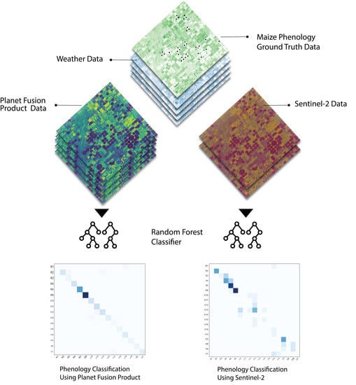
2. Materials and Methods

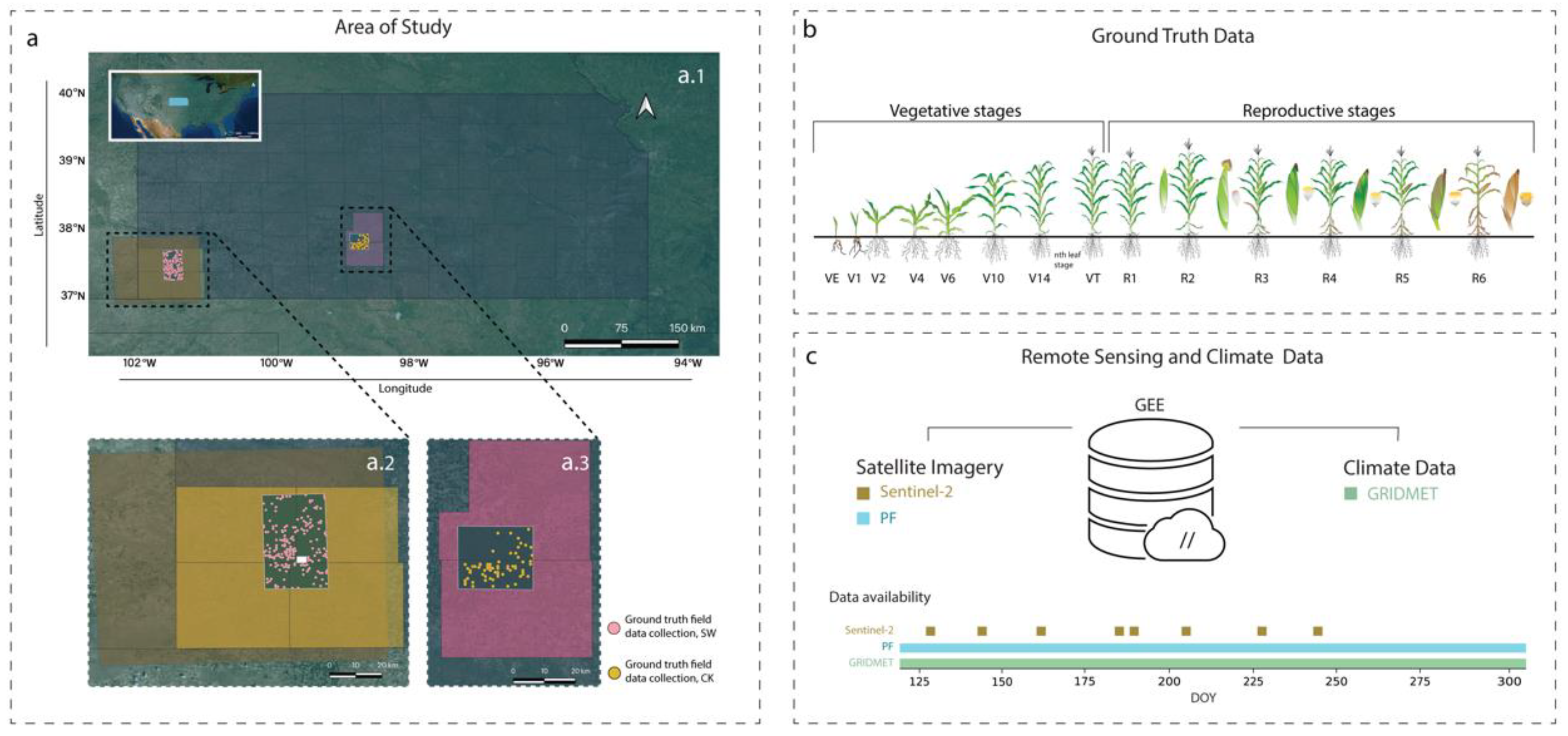
2.1. Study Area

The present study was conducted in the state of Kansas (US) within the Southwest (SW) region comprising the counties of Morton, Stanton, Grant, and Stevens and the Central (CK) region constituted by the counties of Stafford and Pratt (Figure 1a).

The precipitation pattern in Kansas is highly uneven in both quantity and distribution, ranging from over 1000 mm from the southeast to less than 300 mm in the west region of the state. For the two regions selected in this study, these levels ranged from 500 to 800 mm for the CK (rainfed region) and from 300 to 500 mm for the SW region [30]. The size of the fields, as well as standard management practices such as ground water irrigation, differ in these two regions. The SW region is mostly dominated by larger fields relative to the CK, and a higher number of irrigation pivots (fed from the Ogallala Aquifer), resulting in higher maize yields averaging 11 Mg ha⁻¹ for year 2019 [12]. In contrast, the CK region is characterized by smaller fields and mainly dominated by rainfed agriculture with an average maize yield of 9 Mg ha⁻¹ for the year 2019 [12].

2.2. Data Characteristics

2.2.1. Reference Ground Field Data

Acquiring quality environmental data may be challenging and expensive, even more when dealing with extensive geographic areas [31,32]. This requires not just data collection and subsequent storage, but also the training of a person capable of delivering the information with minimal to no bias or errors. Despite these substantial obstacles, ground-truth field data continue to be the most reliable and closest to the true condition of the system [33,34]. For this study, we were able to acquire a valuable source of ground-truth data from Crop Quest Inc., which included geolocated fields spanning many states in the Central region of the United States. This data set was developed during a five-year period, from 2013 to 2017, by conducting repeated trips to each farmer field to document maize crop phenology changes during the growing season. Only the growing season 2017 was analyzed in the present manuscript due to a conjunction of events, related to the sources of information.

On average, each field was visited 5 times during the season; although, this varied within all field observation collected and summarized in this large database. The crop phenology stages present in the data set followed the scale described on Figure 1b, based on [35]. The final database included geolocated fields for both regions, crop phenology measurements per field, and the date of data collection (time stamp).

2.2.2. Remote Sensing Data and Weather Variables

Google Earth Engine (GEE) was used to retrieve and analyze spectral remote sensing data, as well as for the weather information (Figure 1c). This cloud-based platform enabled the processing of large data sets and provided access to a wide library of pre-processed satellite images, climate, and land cover data, as well as built-in algorithms and vector data [36,37].

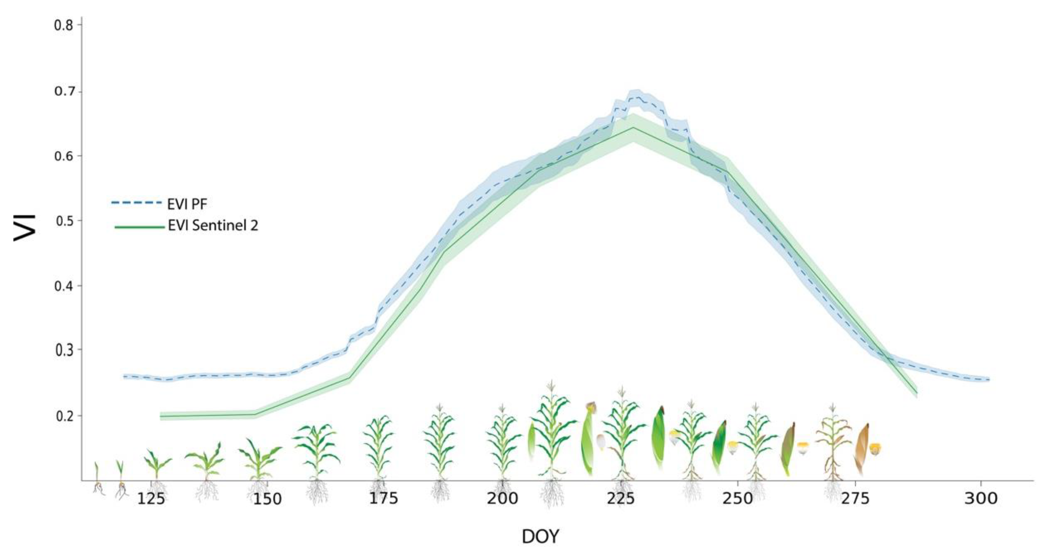
Planet Fusion Product

For the 2017 season, our industry partner provided daily, 3 m resolution, Planet Fusion (PF) Surface Reflectance (SR) data [38]. Planet Fusion constitutes a comprehensive fusion methodology based on the CESTEM algorithm [39,40] to inter-calibrate, harmonize, enhance, and fuse multi-sensor data streams leveraging rigorously calibrated public mission (i.e., Sentinel-2, Landsat 8, MODIS, and VIIRS) products in concert with the higher spatial and temporal resolution CubeSat images from the PlanetScope constellations. PF uses the Framework for Operational Radiometric Correction for Environmental Monitoring (FORCE) [41] to generate a harmonized Sentinel-2 and Landsat 8 BRDF adjusted SR product to be used as the calibration target during the CESTEM-based harmonization step. Additional PF features include: (1) sub-pixel fine geometric alignment of source imagery; (2) rigorous, temporally driven, cloud and cloud shadow detection; (3) fusion of Sentinel-2 and Landsat 8 data to help fill gaps in PlanetScope coverage; and (4) advanced gap-filling. PF delivers daily, gap-filled, 4-band (0.45–0.51, 0.53–0.59, 0.64–0.67, and 0.85–0.88 µm) sensor agnostic SR data characterized by enhanced radiometric stability and consistency across space and time to support advanced analytics. The PF data were provided with a 3 m pixel size as regularly gridded raster tiles (24 by 24 km) in UTM projection.

Due to the high temporal frequency, spatial resolution, and quality of data, this product could prove to be an excellent resource for dealing with detailed crop phenology and its temporal variation. For the SW region, tiles 11E-172 N and 11E-173 N were utilized, as well as tile 21E-174 N for the CK region. Both spectral and associated metadata from each tile were uploaded to GEE via the Google Cloud Repository and organized into a collection for convenient access during feature extraction.

Sentinel-2

Sentinel-2 (S-2) is an optical satellite constellation developed by the European Space Agency (ESA) that is composed of two complementary spacecraft (S-2A and S-2B). This constellation was chosen to compare the PF product to a publicly available, well-studied, and widely reported satellite with a high temporal resolution (median average revisit intervals of 3.7 days, [42]) and spatial resolution (10, 20, and 60 m, [43]).

Tile T14SKG covering southwest Kansas, was used to generate level-2A surface reflectance data using the Sen2Cor processor [44]. This operation was carried out manually using the Sentinel Application Platform (SNAP) and the Sen2Cor plugin (version 2.8), as not all tiles for level-2A are available from the GEE archives for the year 2017 over the state of Kansas. Once the images were converted to bottom of atmosphere reflectance, they were uploaded to GEE for the purpose of calculating the various vegetation indices.

Even though 12 images were produced for the 2017 growing season, only eight of them showed less than 20% cloud cover, and only five of them were time corresponding with observations made during the ground truth field data gathering.

Spectral Bands and Vegetation Indices

A suite of Vegetation indices (VI) including the Normalized Difference Vegetation Index (NDVI), Enhanced Vegetation Index (EVI), Green Chlorophyll Vegetation Index (GCVI), Chlorophyll Vegetation Index (CVI), and Normalized Green Index (NGI) were calculated based on the spectral bands from both products (PF and S-2). Extensive literature is associated with these indices and their capability to monitor vegetation dynamics [45,46,47,48,49].

NDVI is supported by the fact that green/healthy vegetation will have a higher reflectance in the near infrared (NIR) while absorbing in the red band due to the chlorophyll content in the leaf [46]. While extensively utilized, it is well established that this indicator saturates at intermediate biomass levels, owing mostly to its limited sensitivity to elevated chlorophyll concentrations, especially problematic in maize fields. The EVI integrates the blue band to limit the impact of certain atmospheric phenomena and more precisely capture changes in plant canopy, particularly under high productivity areas [50,51], making this vegetation index as an effective alternative to the problem from using NDVI. GCVI has been proven to present a greater linear connection with the leaf area index of maize than other indices and, unlike NDVI, does not saturate as quickly at high biomass levels [48]. Lastly, both CVI and NGI have been widely used due to their responsiveness to changes in the chlorophyll content of the crop [52,53].

Weather Variables

Weather variables were derived from the GEE archives based on gridded surface meteorological data (GRIDMET), [54]. This data set integrates high-resolution spatial data from PRISM (2.5 arc minute, 4 km) with regular temporal resolution data from the North American Land Data Assimilation System (NLDAS) [55]. The main meteorological variables retrieved for the analysis were mean, minimum, and maximum temperatures, precipitation, and vapor pressure deficit (VPD), all on a daily temporal scale.

2.3. Data Preparation

To extract circular fields linked to irrigated pivot operations, the Canny edge detector [56] method was implemented on the GEE platform. Using this mask, in conjunction with the fields under study, we were able to construct a layer that included information about the geolocation and phenology of each irrigation field in the data set. As a result, the mean values of the spectral bands (red, green, blue, and NIR), VIs (NDVI, EVI, GCVI, CVI, and NGI), and the weather parameters (precipitation, minimum temperature, maximum temperature, and VPD) associated with each field for each given date were all gathered to construct the main database with both sensors.

Despite PF daily availability, only images day-coincident with the ground-based phenology collections (a total of 91 dates) were utilized (Figure 2). These dates were distributed between 1 May and 30 October. The same method was applied to S-2 data after filtering based on a cloud mask with a cloud threshold less or equal to 20%. During that process, S-2 images with less than 20% cloud cover were retained for the analyses. With this filtering protocol, only five S-2 images (dates: 15 June, 30 June, 5 July, 25 July, and 14 August) were available on the same date as the phenology collections (Figure 2). Due to this temporal limitation, additional studies were conducted to also consider phenology data acquired within 3 and 10 days of the image collection. As a result, this stage of the study analyzed three data sets: (i) containing the spectral band values, VIs, and weather parameters for the exact phenology date; (ii) same parameters as in (i) spanning three days before and after the crop phenology collection date (7 days total); and (iii) same parameters as in (i) ranging ten days before and after the crop phenology collection date (21 days total).

2.4. Random Forest

The Random Forest (RF) classifier was implemented with the Scikit-Learn library [57], in a Python 3.8 environment. RF represents a supervised classifier, learning from training samples; thus, the quality of training instances is a key component in the classification process. The RF classifier, in addition, is an ensemble classifier, in which multiple decision trees are utilized to improve generalizability and, therefore, resilience by using a randomly selected subset of training samples and variables [58]. All these aspects contribute to the creation of accurate classifications, as well as the processing of large amounts of data. It has been utilized in remote sensing for more than two decades, proving valuable in the handling of high-dimensional data, unbalanced data sets, and multi-target problems, while remaining simple and adaptable using multiple hyperparameters. [25,26,27,59,60,61].

To produce a more robust model in this study, the hyperparameters were derived based on an exhaustive grid search checking for various values at each hyperparameter and retaining the ones that resulted in the best performance. The data set for this test was created by combining the variables in their final configuration (further details presented in the section below). This resulted in the following hyperparameter values: bootstrap: True; maximum tree depth: 10; maximum number of features required to do the best split: ‘auto’; minimum sample size per leaf: 2; minimum sample size required to execute the split: 2; number of trees: 1000. To evaluate performance, the data sets (PF and S-2) were split into training, validation, and test sections for each experiment. From the total of the data, 70% was used for training purposes and validation (fraction A) and 30% for model assessment (fraction B). Fraction A was further divided into 70% for training (fraction Aa) and 30% for validation (fraction Ab).

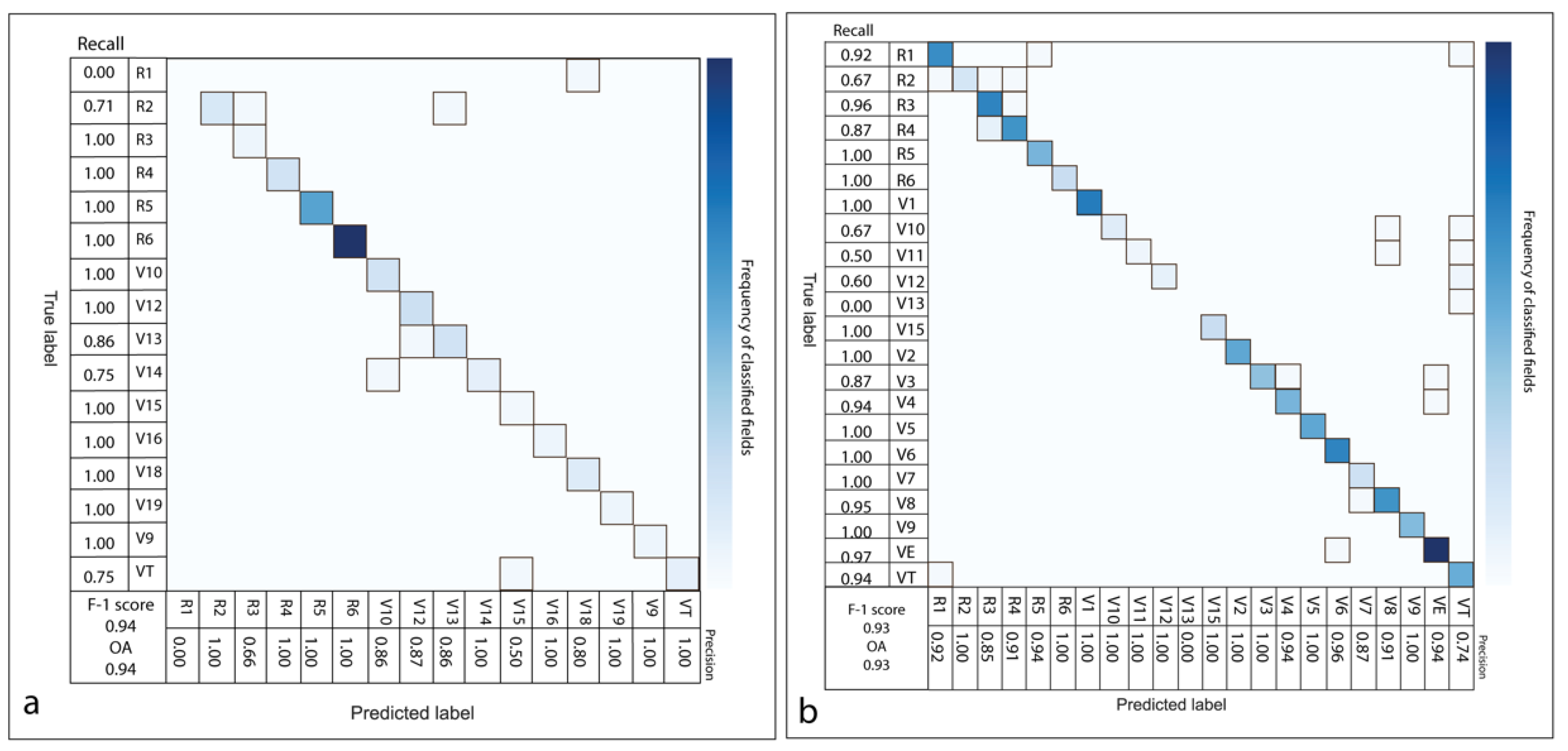
2.4.1. Performance Metrics

When evaluating the performance of RF, the most commonly used metrics are overall accuracy, precision, recall, and F1-score [62]. Considering the examples in the literature we can obtain these metrics following the Equations (1)–(4) [63]. Most of the literature studying the performance of these metrics is centered on balanced binary classifications. In this paper, the ground-truth data set presents more than 18 classes, where each class does not contain the same number of samples. According to [64], F1-score, defined as the harmonic mean of precision and recall, can be a useful metric to use with respect to unbalanced data sets. In contrast, the use of overall accuracy, the total of correctly identified elements divided by total number of elements to be classified, can be misleading since it will favor the most represented class [65]. Precision represents the fraction of samples assigned to the class that are in fact part of the class, and recall represents how well the class was predicted.

$$accuracy=\frac{True positives+True negatives}{All samples}$$

(1)

$$precision=\frac{True positives }{True positives+False positives}$$

(2)

$$recall=\frac{True positives}{True positives+False negatives}$$

(3)

$$F1 score=\frac{Precision x Recall}{Precision+Recall}$$

(4)

2.4.2. Feature Importance

In classification tasks, feature selection is commonly used to reduce the dimensionality of the data set [26,66] and to inform on the relative influence of each variable in the model. To narrow down the possible combinations of variables to produce the best classifier, a feature importance analysis was conducted based on the PF data set, for both the SW and CK regions. For this purpose, all the variables (VIs, spectral bands, weather data, geolocation of the fields, and day of the year of field collections) were utilized.

3. Results

3.1. Best Combination of Variables

The analysis of the feature importance from the SW region data set revealed that NIR band (B4) and EVI, as well as the minimum and maximum temperatures (Tmin and Tmax), VPD, and DOY, were associated with the highest scores. When all the variables were combined, we found that the best f1-scores were 0.94 for the SW region and 0.93 for the CK region. Additionally, and to investigate other model possibilities, several combinations were attempted (only spectral data; only weather parameters; EVI and weather; B4 and weather, etc.). The lowest f1-scores were derived when the model was only driven by weather variables, with 0.79 for SW and 0.76 for CK regions.

3.2. Model Performance Using PF Data in Both Regions

The model including NIR, EVI, Tmin, Tmax, VPD, and DOY was utilized to classify regions, yielding f1 values of 0.94 for the SW and 0.93 for the CK regions (Figure 3a,b). The classification results for each crop phenological stage are presented as a confusion matrix, where all the components that were correctly identified are along the main diagonal, as well as the resulting precision and recall along the X and Y axes. When examining the SW area in detail, most of stages produced values between 1.0 and 0.75 (recall) and 1.0 to 0.80 (precision), whereas certain stages, such as R1, R3, and V15, showed poor metrics ranging from 0 to 0.66. Similarly, the findings for the CK region showed that most stages had recall values ranging from 1.0 to 0.87, but some (R2, V10, V11, V12, and V13) exhibited recall values below 0.67. When the precision is considered, all stages ranged from 0.76 to 1.0.

3.3. Model Performance Using Sentinel-2 Data

When the same model was applied to S-2 data, the findings were inferior to those previously discussed in this paper. The first data set included just three crop phenological stages, due to the season timeframe captured by the images. The classification resulted in an overall high f1-score (0.86), but inconsistent metrics for each stage, for example, for VT stage both recall and precision were zero (Figure 4a). As a second step, the performance of the extended data set, including data from 3 days before and after the time of field data collection, was tested. In this experiment, the overall f1-score was reduced to 0.74 but more phenological stages were part of the data set. Lastly, the test was repeated by expanding the search from 3 to 10 days before and after the field data collection time. This resulted in an f1-score of 0.58 with several crop phenology stages still not classified (null metrics). When the S-2 data set was employed, the overall performance was consistently inferior to when the PF product was utilized (Figure 4).

4. Discussion

This study demonstrates the benefits of having access to high-cadence earth observation at both spatio-temporal dimensions. This analysis employs a simple model trained on spectral characteristics, meteorological variables, and high-quality ground truth labels to achieve optimal crop phenology classification, using maize crop in this US region as testbed for this case study. The findings presented in this study are in accordance with those observed when tracking crop phenology [1,13,66,67,68], most notably the importance of enhanced temporal resolution [9,10,69].

This combination of variables resulted in overall classification metrics higher than 0.90, with each phenological stage identified accurately as described in sections above. Despite the disparities in the characterization of both regions under analysis (SW and CK) in terms of climate, field size, and average yield, the model performance was similar for both areas using the same combination of variables. Previous studies have highlighted the importance of VIs when monitoring changes in crop phenology, and particularly EVI has been found to outperform a broad variety of VIs in maize fields [61,70,71,72]. In addition, promising results were achieved by [73] relying on the NIR band. On the other hand, inclusion of relevant weather variables is crucial to describing changes in crop phenology and development, as demonstrated in modeling scenarios [74,75], with air temperature among the most relevant variables [76]. In addition, VPD has been strongly associated with water stress and the consequent impact on crop development [77,78].

This study also highlights the relevancy of high-cadence satellite data for classifying crop phenology more accurately. Due to cloud cover only a few S-2 images were available during the 2017 growing season. This significantly reduced the likelihood of finding an image acquired on the same day as the field data collection, which affected the ability to classify the crop phenology stages. In order to emphasize the importance of temporal resolution for this purpose, a sensitivity analysis using PF data only was conducted evaluating the performance implications of excluding data from within 1, 2, and 3 days of the date of the field data collection, respectively. The ability of the classifier to achieve high prediction metrics was substantially reduced by 12% with the 2-day, and by roughly more than 40%, with the 3-day departure, especially during crop developmental phases around the time of flowering (e.g., V12, V13, and V19). These results emphasize the importance of having access to low-latency spectral data, particularly during periods of rapid crop growth.

Potential caveats and uncertainties from the analysis are related to problems associated with multiclass classification and imbalanced data sets. Most of the methods to treat imbalanced data sets rely on binary problems [79] and solutions are not extensively proven. Having access to daily spectral data as well as increasing the number of ground truth samples represent key factors in the attempt to build more reliable predictions. In this study, this was partially overcome using the daily PF product that resulted in very robust and consistent classification results. More efforts are being conducted towards the development and availability of fusion products, such as the Harmonized Landsat-Sentinel (HLS); although, it was not implemented on this analysis since, at the time, it was suggested to not be yet used for scientific purposes [80].

Further research should focus on verifying the existing model on smaller scales (e.g., smallholder farms) to determine its transferability to more complex farming systems and management approaches, as well as its contribution to precision agriculture initiatives [81,82]. Additionally, since this study focused only on maize, a crop with well-defined stages, further research incorporating soybeans, sorghum, and sunflower, among others, should be explored. Extending the research period to include seasonal weather scenarios representative of current and future climatic conditions (e.g., heat, drought, and changes in rain patterns) in the context of climate change is another critical avenue to pursue, as is examining the influence of hyperspectral data from DECIS, HISUI, PRISMA, and future CHIME, and SBG missions [83].

5. Conclusions

A proposed random forest model combining satellite-based (NIR band surface reflectance, and EVI), weather data (maximum and minimum temperatures, and VPD), and day of the year enabled a high-quality crop phenology classification for maize crops under two contrasting production regions. The study highlights the critical importance of having access to high-cadence earth observation, as well as high-quality ground truth data. Classification accuracy was shown to decrease significantly when comparing performance metrics from a scenario with limited temporal availability (S-2 clear-sky images) with a daily data scenario (Planet Fusion product), particularly when the same image was used to make inferences about the future or the past. In summary, this study successfully portrayed the spatial transferability of this satellite- and weather-based crop phenology model applied to contrasting maize producing regions while preserving performance. Therefore, this simple crop phenology model can become a promising tool that still needs to be globally tested.

Most of the existing crop phenology solutions rely on broad metrics as well as large geographic regions. While these are important tools for policymakers and governments to use when making global or regional decisions, there is still room for development in terms of farmer solutions. Additionally, these measurements do not reflect the crop’s real status but rather the vegetation’s spectral information. This discrepancy between what is reported and what occurs in the field might result in misconceptions and incorrect conclusions. Improving crop phenology classification and reporting has a substantial influence on every step of the food production chain, enabling accurate, proactive, rather than reactive, strategies at the regional and field level.

References

1. Liang, L.; Schwartz, M.D.; Fei, S. Validating satellite phenology through intensive ground observation and landscape scaling in a mixed seasonal forest. Remote Sens. Environ. 2011, 115, 143–157. [Google Scholar] [CrossRef]
2. Ruml, M.; Vulić, T. Importance of phenological observations and predictions in agriculture. J. Agric. Sci. 2005, 50, 217–225. [Google Scholar] [CrossRef]
3. Henebry, G.M.; de Beurs, K.M. Remote Sensing of Land Surface Phenology: A Prospectus. In Phenology: An Integrative Environmental Science; Springer: Dordrecht, The Netherlands, 2013; pp. 385–411. [Google Scholar]
4. Sakamoto, T.; Wardlow, B.D.; Gitelson, A.A.; Verma, S.B.; Suyker, A.E.; Arkebauer, T.J. A two-step filtering approach for detecting maize and soybean phenology with time-series MODIS data. Remote Sens. Environ. 2010, 114, 2146–2159. [Google Scholar] [CrossRef]
5. Wang, H.; Ghosh, A.; Linquist, B.A.; Hijmans, R.J. Satellite-Based Observations Reveal Effects of Weather Variation on Rice Phenology. Remote Sens. 2020, 12, 1522. [Google Scholar] [CrossRef]
6. Li, S.; Xiao, J.; Ni, P.; Zhang, J.; Wang, H.; Wang, J. Monitoring paddy rice phenology using time series MODIS data over Jiangxi Province, China. Int. J. Agric. Biol. Eng. 2014, 7, 28–36. [Google Scholar]
7. Rezaei, E.E.; Siebert, S.; Hüging, H.; Ewert, F. Climate change effect on wheat phenology depends on cultivar change. Sci. Rep. 2018, 8, 4891. [Google Scholar] [CrossRef] [PubMed] [Green Version]
8. Sharifi, H.; Hijmans, R.J.; Hill, J.E.; Linquist, B.A. Using Stage-Dependent Temperature Parameters to Improve Phenological Model Prediction Accuracy in Rice Models. Crop Sci. 2017, 57, 444–453. [Google Scholar] [CrossRef] [Green Version]
9. Gao, F.; Zhang, X. Mapping crop phenology in near real-time using satellite remote sensing: Challenges and opportunities. J. Remote Sens. 2021, 2021, 8379391. [Google Scholar] [CrossRef]
10. Gao, F.; Anderson, M.C.; Zhang, X.; Yang, Z.; Alfieri, J.G.; Kustas, W.P.; Mueller, R.; Johnson, D.M.; Prueger, J.H. Toward mapping crop progress at field scales through fusion of Landsat and MODIS imagery. Remote Sens. Environ. 2017, 188, 9–25. [Google Scholar] [CrossRef] [Green Version]
11. United States Department of Agriculture. USDA. 2018. Available online: https://www.nass.usda.gov/Statistics_by_State/Kansas/Publications/Crop_Progress_and_Condition/historic.php (accessed on 20 December 2021).
12. USDA/NASS Quickstats. Available online: https://quickstats.nass.usda.gov/ (accessed on 15 July 2021).
13. White, M.A.; Thornton, P.E.; Running, S.W. A continental phenology model for monitoring vegetation responses to interannual climatic variability. Glob. Biogeochem. Cycles 1997, 11, 217–234. [Google Scholar] [CrossRef]
14. Zhang, X.; Friedl, M.A.; Schaaf, C.B.; Strahler, A.H.; Hodges, J.C.; Gao, F.; Reed, B.C.; Huete, A. Monitoring vegetation phenology using MODIS. Remote Sens. Environ. 2003, 84, 471–475. [Google Scholar] [CrossRef]
15. Vina, A.; Gitelson, A.A.; Rundquist, D.C.; Keydan, G.P.; Leavitt, B.; Schepers, J. Monitoring maize (Zea mays L.) phenology with remote sensing. Agron. J. 2004, 96, 1139–1147. [Google Scholar] [CrossRef]
16. Houborg, R.; Fisher, J.B.; Skidmore, A.K. Advances in remote sensing of vegetation function and traits. Int. J. Appl. Earth Obs. Geoinf. 2015, 43, 1–6. [Google Scholar] [CrossRef] [Green Version]
17. Rast, M.; Painter, T.H. Earth observation imaging spectroscopy for terrestrial systems: An overview of its history, techniques, and applications of its missions. Surv. Geophys. 2019, 40, 303–331. [Google Scholar] [CrossRef]
18. Wulder, M.A.; Loveland, T.R.; Roy, D.P.; Crawford, C.J.; Masek, J.G.; Woodcock, C.E.; Allen, R.G.; Anderson, M.C.; Belward, A.S.; Cohen, W.B.; et al. Current status of Landsat program, science, and applications. Remote Sens. Environ. 2019, 225, 127–147. [Google Scholar] [CrossRef]
19. Claverie, M.; Ju, J.; Masek, J.G.; Dungan, J.L.; Vermote, E.F.; Roger, J.C.; Skakun, S.V.; Justice, C. The Harmonized Landsat and Sentinel-2 surface reflectance data set. Remote Sens. Environ. 2018, 219, 145–161. [Google Scholar] [CrossRef]
20. Liao, C.; Wang, J.; Dong, T.; Shang, J.; Liu, J.; Song, Y. Using spatio-temporal fusion of Landsat-8 and MODIS data to derive phenology, biomass and yield estimates for corn and soybean. Sci. Total Environ. 2019, 650, 1707–1721. [Google Scholar] [CrossRef]
21. Arun, P.V.; Sadeh, R.; Avneri, A.; Tubul, Y.; Camino, C.; Buddhiraju, K.M.; Porwal, A.; Lati, R.; Zarco-Tejada, P.; Peleg, Z.; et al. Multimodal Earth observation data fusion: Graph-based approach in shared latent space. Inf. Fusion 2022, 78, 20–39. [Google Scholar] [CrossRef]
22. Schramowski, P.; Stammer, W.; Teso, S.; Brugger, A.; Herbert, F.; Shao, X.; Luigs, H.-G.; Mahlein, A.-K.; Kersting, K. Making deep neural networks right for the right scientific reasons by interacting with their explanations. Nat. Mach. Intell. 2020, 2, 476–486. [Google Scholar] [CrossRef]
23. Gislason, P.O.; Benediktsson, J.A.; Sveinsson, J.R. Random forests for land cover classification. Pattern Recognit. Lett. 2006, 27, 294–300. [Google Scholar] [CrossRef]
24. Breiman, L. Random forests. Mach. Learn. 2001, 45, 5–32. [Google Scholar] [CrossRef] [Green Version]
25. Pal, M. Random forest classifier for remote sensing classification. Int. J. Remote Sens. 2005, 26, 217–222. [Google Scholar] [CrossRef]
26. Rodriguez-Galiano, V.F.; Ghimire, B.; Rogan, J.; Chica-Olmo, M.; Rigol-Sanchez, J.P. An assessment of the effectiveness of a random forest classifier for land-cover classification. ISPRS J. Photogramm. Remote Sens. 2012, 67, 93–104. [Google Scholar] [CrossRef]
27. Belgiu, M.; Drăguţ, L. Random forest in remote sensing: A review of applications and future directions. ISPRS J. Photogramm. Remote Sen. 2016, 114, 24–31. [Google Scholar] [CrossRef]
28. Fernández-Delgado, M.; Cernadas, E.; Barro, S.; Amorim, D. Do we need hundreds of classifiers to solve real world classification problems? J. Mach. Learn. Res. 2014, 15, 3133–3181. [Google Scholar]
29. Rodriguez-Galiano, V.; Sanchez-Castillo, M.; Chica-Olmo, M.; Chica-Rivas, M. Machine learning predictive models for mineral prospectivity: An evaluation of neural networks, random forest, regression trees and support vector machines. Ore Geol. Rev. 2015, 71, 804–818. [Google Scholar] [CrossRef]
30. Lin, X.; Harrington, J.; Ciampitti, I.; Gowda, P.; Brown, D.; Kisekka, I. Kansas trends and changes in temperature, precipitation, drought, and frost-free days from the 1890s to 2015. J. Contemp. Water Res. Educ. 2017, 162, 18–30. [Google Scholar] [CrossRef] [Green Version]
31. Hanks, E.M.; Hooten, M.B.; Baker, F.A. Reconciling multiple data sources to improve accuracy of large-scale prediction of forest disease incidence. Ecol. Appl. 2011, 21, 1173–1188. [Google Scholar] [CrossRef] [PubMed]
32. Ruiz-Gutierrez, V.; Hooten, M.B.; Grant, E.H.C. Uncertainty in biological monitoring: A framework for data collection and analysis to account for multiple sources of sampling bias. Methods Ecol. Evol. 2016, 7, 900–909. [Google Scholar] [CrossRef] [Green Version]
33. Hooten, M.B.; Wikle, C.K.; Dorazio, R.M.; Royle, J.A. Hierarchical spatiotemporal matrix models for characterizing invasions. Biometrics 2007, 63, 558–567. [Google Scholar] [CrossRef]
34. Dickinson, J.L.; Shirk, J.; Bonter, D.; Bonney, R.; Crain, R.L.; Martin, J.; Phillips, T.; Purcell, K. The current state of citizen science as a tool for ecological research and public engagement. Front. Ecol. Environ. 2012, 10, 291–297. [Google Scholar] [CrossRef] [Green Version]
35. Ciampitti, I.A.; Elmore, R.W.; Lauer, J. Corn Growth and Development; KSRE Bookstore: Manhattan, KS, USA, 2016; Available online: https://bookstore.ksre.ksu.edu/pubs/MF3305.pdf (accessed on 15 January 2022).
36. Gorelick, N.; Hancher, M.; Dixon, M.; Ilyushchenko, S.; Thau, D.; Moore, R. Google Earth Engine: Planetary-scale geospatial analysis for everyone. Remote Sens. Environ. 2017, 202, 18–27. [Google Scholar] [CrossRef]
37. Kumar, L.; Mutanga, O. Google Earth Engine applications since inception: Usage, trends, and potential. Remote Sen. 2018, 10, 1509. [Google Scholar] [CrossRef] [Green Version]
38. Planet Fusion Team. Planet Fusion Monitoring Technical Specification, Version 1.0.0-beta.3, San Francisco, CA, USA. 2021. Available online: https://assets.planet.com/docs/Planet_fusion_specification_March_2021.pdfD (accessed on 1 April 2021).
39. Houborg, R.; McCabe, M.F. Daily Retrieval of NDVI and LAI at 3 m Resolution via the Fusion of CubeSat, Landsat, and MODIS Data. Remote Sens. 2018, 10, 890. [Google Scholar] [CrossRef] [Green Version]
40. Houborg, R.; McCabe, M.F. A Cubesat Enabled Spatio-Temporal Enhancement Method (CESTEM) utilizing Planet, Landsat and MODIS data. Remote Sens. Environ. 2018, 209, 211–226. [Google Scholar] [CrossRef]
41. Frantz, D. FORCE—Landsat + Sentinel-2 analysis ready data and beyond. Remote Sens. 2019, 11, 1124. [Google Scholar] [CrossRef] [Green Version]
42. Li, J.; Roy, D.P. A global analysis of Sentinel-2A, Sentinel-2B and Landsat-8 data revisit intervals and implications for terrestrial monitoring. Remote Sen. 2017, 9, 902. [Google Scholar] [CrossRef] [Green Version]
43. Drusch, M.; Del Bello, U.; Carlier, S.; Colin, O.; Fernandez, V.; Gascon, F.; Hoersch, B.; Isola, C.; Labergellinti, P.; Martimort, P.; et al. Sentinel-2: ESA’s optical high-resolution mission for GMES operational services. Remote Sens. Environ. 2012, 120, 25–36. [Google Scholar] [CrossRef]
44. Main-Knorn, M.; Pflug, B.; Louis, J.; Debaecker, V.; Müller-Wilm, U.; Gascon, F. Sen2Cor for Sentinel-2. In Image and Signal Processing for Remote Sensing XXIII. Int. Soc. Opt. Photonics 2017, 10427, 1042704. [Google Scholar]
45. Tucker, C.J. Asymptotic nature of grass canopy spectral reflectance. Appl. Opt. 1977, 16, 1151–1156. [Google Scholar] [CrossRef]
46. Tucker, C.J. Red and photographic infrared linear combinations for monitoring vegetation. Remote Sens. Environ. 1979, 8, 127–150. [Google Scholar] [CrossRef] [Green Version]
47. Turner, D.P.; Cohen, W.B.; Kennedy, R.E.; Fassnacht, K.S.; Briggs, J.M. Relationships between leaf area index and Landsat TM spectral vegetation indices across three temperate zone sites. Remote Sens. Environ. 1999, 70, 52–68. [Google Scholar] [CrossRef]
48. Gitelson, A.A.; Vina, A.; Arkebauer, T.J.; Rundquist, D.C.; Keydan, G.; Leavitt, B. Remote estimation of leaf area index and green leaf biomass in maize canopies. Geophys. Res. Lett. 2003, 30, 1248. [Google Scholar] [CrossRef] [Green Version]
49. Viña, A.; Gitelson, A.A.; Nguy-Robertson, A.L.; Peng, Y. Comparison of different vegetation indices for the remote assessment of green leaf area index of crops. Remote Sens. Environ. 2011, 115, 3468–3478. [Google Scholar] [CrossRef]
50. Liu, H.Q.; Huete, A. A feedback-based modification of the NDVI to minimize canopy background and atmospheric noise. IEEE Transac. Geosci. Remote Sen. 1995, 33, 457–465. [Google Scholar] [CrossRef]
51. Huete, A.; Didan, K.; Miura, T.; Rodriguez, E.P.; Gao, X.; Ferreira, L.G. Overview of the radiometric and biophysical performance of the MODIS vegetation indices. Remote Sen. Environ. 2002, 83, 195–213. [Google Scholar] [CrossRef]
52. Vincini, M.; Frazzi, E. Comparing narrow and broad-band vegetation indices to estimate leaf chlorophyll content in planophile crop canopies. Precis. Agric. 2011, 12, 334–344. [Google Scholar] [CrossRef]
53. Sripada, R.P.; Heiniger, R.W.; White, J.G.; Meijer, A.D. Aerial color infrared photography for determining early in-season nitrogen requirements in corn. Agron. J. 2006, 98, 968–977. [Google Scholar] [CrossRef]
54. Abatzoglou, J.T. Development of gridded surface meteorological data for ecological applications and modelling. Int. J. Climatol. 2013, 33, 121–131. [Google Scholar] [CrossRef]
55. Abatzoglou, J.T.; Rupp, D.E.; Mote, P.W. Seasonal climate variability and change in the Pacific Northwest of the United States. J. Clim. 2014, 27, 2125–2142. [Google Scholar] [CrossRef]
56. Canny, J.F. A computation approach to edge detection. IEEE Trans. Pattern Anal. Mach. Intell. 1986, 8, 670–700. [Google Scholar]
57. Pedregosa, F.; Varoquaux, G.; Gramfort, A.; Michel, V.; Thirion, B.; Grisel, O.; Blondel, M.; Prettenhofer, P.; Weiss, R.; Dubourg, V.; et al. Scikit-learn: Machine learning in Python. J. Mach. Learn. Res. 2011, 12, 2825–2830. [Google Scholar]
58. Dietterich, T.G. Ensemble Methods in Machine Learning. In Proceedings of the International Workshop on Multiple Classifier Systems, Cagliari, Italy, 21–23 June 2000; pp. 1–15. [Google Scholar]
59. Gómez, C.; White, J.C.; Wulder, M.A. Optical remotely sensed time series data for land cover classification: A review. ISPRS J. Photogramm. Remote Sens. 2016, 116, 55–72. [Google Scholar] [CrossRef] [Green Version]
60. Pelletier, C.; Valero, S.; Inglada, J.; Champion, N.; Dedieu, G. Assessing the robustness of Random Forests to map land cover with high resolution satellite image time series over large areas. Remote Sens. Environ. 2016, 187, 156–168. [Google Scholar] [CrossRef]
61. Tatsumi, K.; Yamashiki, Y.; Torres MA, C.; Taipe, C.L.R. Crop classification of upland fields using Random Forest of time-series Landsat ETM+ data. Comput. Electron. Agric. 2015, 115, 171–179. [Google Scholar] [CrossRef]
62. Congalton, R.G. A review of assessing the accuracy of classifications of remotely sensed data. Remote Sens. Environ. 1991, 37, 35–46. [Google Scholar] [CrossRef]
63. Goutte, C.; Gaussier, E. A Probabilistic Interpretation of Precision, Recall and F-Score, With Implication for Evaluation. In Proceedings of the European Conference on Information Retrieval, Lisbon, Portugal, 4–17 April 2005; pp. 345–359. [Google Scholar]
64. Branco, P.; Torgo, L.; Ribeiro, R.P. A survey of predictive modeling on imbalanced domains. ACM Comput. Surv. 2016, 49, 1–50. [Google Scholar] [CrossRef]
65. Nguyen, G.H.; Bouzerdoum, A.; Phung, S.L. Learning Pattern Classification Tasks with Imbalanced Data Sets; IntechOpen Limited: London, UK, 2009; pp. 193–208. Available online: https://www.intechopen.com/chapters/9154 (accessed on 15 January 2022).
66. Peng, B.; Guan, K.; Pan, M.; Li, Y. Benefits of seasonal climate prediction and satellite data for forecasting US maize yield. Geophys. Res. Lett. 2018, 45, 9662–9671. [Google Scholar] [CrossRef]
67. Bandaru, V.; Yaramasu, R.; Koutilya, P.N.V.R.; He, J.; Fernando, S.; Sahajpal, R.; Wardlow, B.D.; Suyker, A.; Justice, C. PhenoCrop: An integrated satellite-based framework to estimate physiological growth stages of corn and soybeans. Int. J. Appl. Earth Observ. Geoinf. 2020, 92, 102188. [Google Scholar] [CrossRef]
68. Nieto, L.; Schwalbert, R.; Prasad, P.V.; Olson, B.J.; Ciampitti, I.A. An integrated approach of field, weather, and satellite data for monitoring maize phenology. Sci. Rep. 2021, 11, 15711. [Google Scholar] [CrossRef] [PubMed]
69. Gao, F.; Anderson, M.; Daughtry, C.; Karnieli, A.; Hively, D.; Kustas, W. A within-season approach for detecting early growth stages in corn and soybean using high temporal and spatial resolution imagery. Remote Sens. Environ. 2020, 242, 111752. [Google Scholar] [CrossRef]
70. Zhong, L.; Hu, L.; Yu, L.; Gong, P.; Biging, G.S. Automated mapping of soybean and corn using phenology. ISPRS J. Photogramm. Remote Sens. 2016, 119, 151–164. [Google Scholar] [CrossRef] [Green Version]
71. Zhong, L.; Yu, L.; Li, X.; Hu, L.; Gong, P. Rapid corn and soybean mapping in US Corn Belt and neighboring areas. Sci. Rep. 2016, 6, 36240. [Google Scholar] [CrossRef] [Green Version]
72. Cai, Y.; Guan, K.; Lobell, D.; Potgieter, A.B.; Wang, S.; Peng, J.; Xu, T.; Asseng, S.; Zhang, Y.; You, L.; et al. Integrating satellite and climate data to predict wheat yield in Australia using machine learning approaches. Agric. For. Meteorol. 2019, 274, 144–159. [Google Scholar] [CrossRef]
73. Cai, Y.; Guan, K.; Peng, J.; Wang, S.; Seifert, C.; Wardlow, B.; Li, Z. A high-performance and in-season classification system of field-level crop types using time-series Landsat data and a machine learning approach. Remote Sens. Environ. 2018, 210, 35–47. [Google Scholar] [CrossRef]
74. Bai, J.; Chen, X.; Dobermann, A.; Yang, H.; Cassman, K.G.; Zhang, F. Evaluation of NASA satellite-and model-derived weather data for simulation of maize yield potential in China. Agron. J. 2010, 102, 9–16. [Google Scholar] [CrossRef]
75. Joshi, V.R.; Kazula, M.J.; Coulter, J.A.; Naeve, S.L.; Garcia, A.G.y. In-season weather data provide reliable yield estimates of maize and soybean in the US central Corn Belt. Int. J. Biometeorol. 2021, 65, 489–502. [Google Scholar] [CrossRef]
76. Azzari, G.; Jain, M.; Lobell, D.B. Towards fine resolution global maps of crop yields: Testing multiple methods and satellites in three countries. Remote Sens. Environ. 2017, 202, 129–141. [Google Scholar] [CrossRef]
77. Zhang, S.; Tao, F.; Zhang, Z. Spatial and temporal changes in vapor pressure deficit and their impacts on crop yields in China during 1980–2008. J. Meteorol. Res. 2017, 31, 800–808. [Google Scholar] [CrossRef]
78. Hsiao, J.; Swann, A.L.; Kim, S.H. Maize yield under a changing climate: The hidden role of vapor pressure deficit. Agric. For. Meteorol. 2019, 279, 107692. [Google Scholar] [CrossRef] [Green Version]
79. Hoens, T.R.; Qian, Q.; Chawla, N.V.; Zhou, Z.H. Building Decision Trees for The Multi-Class Imbalance Problem. In Proceedings of the Pacific-Asia Conference on Knowledge Discovery and Data Mining, Kuala Lumpur, Malaysia, 29 May–1 June 2012; pp. 122–134. [Google Scholar]
80. LP DAAC-HLSL30. (n.d.). LP DAAC-HLSL30. Available online: https://lpdaac.usgs.gov/products/hlsl30v015/ (accessed on 5 August 2021).
81. Mulla, D.J. Twenty five years of remote sensing in precision agriculture: Key advances and remaining knowledge gaps. Biosyst. Eng. 2013, 114, 358–371. [Google Scholar] [CrossRef]
82. Herrmann, I.; Bdolach, E.; Montekyo, Y.; Rachmilevitch, S.; Townsend, P.A.; Karnieli, A. Assessment of maize yield and phenology by drone-mounted superspectral camera. Precis. Agric. 2020, 21, 51–76. [Google Scholar] [CrossRef]
83. Seeley, M.; Asner, G.P. Imaging Spectroscopy for Conservation Applications. Remote Sens. 2021, 13, 292. [Google Scholar] [CrossRef]
Figure 1. (a) Area of study (a.1) state of Kansas (US), (a.2) Southwest (SW) region; the large orange rectangle represents the Sentinel-2 tile covering the area; the green rectangle corresponds with the Planet Fusion (PF) tiles over the area; pink dots represent ground truth field data collection sites, (a.3) Central KS (CK) region; green rectangle corresponds with the PF tile over the area; yellow dots represent ground truth field data collection sites. (b) Maize phenology stages, with the phenology scale used during ground truth data collection, following Ciampitti et al. (2016). (c) Sentinel-2 and PF data imagery and GRIDMET data from the Google Earth Engine (GEE) repository, data availability differs temporally with 8 images collected for Sentinel-2, and daily data for both PF and weather data during the 2017 growing season, varying with the day of the year (DOY).
Remotesensing 14 00469 g001
Figure 2. EVI temporal series for the 2017 maize growing season for SW fields using Sentinel-2 (solid green line) and PF (dash blue line). The shaded area around both lines represent the standard deviation of the EVI values for the fields under study (pink dots Figure 1(a.2)). Maize phenology progress and development stages is depicted on the x-axis.
Remotesensing 14 00469 g002
Figure 3. (a) Confusion matrices with PF-based classification results for the Southwest region (SW) and for (b) Central KS region (CK), including recall and precision for each crop phenology stage, and f1-score and overall accuracy (OA).
Remotesensing 14 00469 g003
Figure 4. Confusion matrices with S-2 based classification results for the Southwest (SW) region, (a) including imagery on the date of data collection, (b) including data within 3 days before and after, (c) including data within 10 days before and after. All matrices include recall and precision for each crop phenology stage, and f1-score and overall accuracy (OA).
Remotesensing 14 00469 g004
Publisher’s Note: MDPI stays neutral with regard to jurisdictional claims in published maps and institutional affiliations.