Abstract
Target three-dimensional (3D) high-resolution imaging via multiple-input multiple-output (MIMO) radar may suffer from a heavy sampling burden and complicated radio frequency interferences. Considering a collocated two-dimensional wideband MIMO radar under dynamic wideband interference (WBI), this paper proposes a cognitive method to achieve a 3D high-resolution target image with a reduced sampling cost. Firstly, based on the known knowledge of the target and WBI, provided by previous measurements, optimal sparse sampling in the 3D signal domain is conducted to reduce the number of sub-pulses and transceiving antennas by solving an optimization problem. Then, the detection and removal of the interfered signal components are conducted to provide the WBI information for following measurements and the interference-free signal cube for the target imaging process. Finally, by using the tensor-based smoothed L0 algorithm, the 3D high-resolution image of the target is obtained, providing the target information for the next measurement. Based on these three steps, a cognitive sparse imaging loop is formed for MIMO radar under WBI situations. The simulation and experiment results demonstrate the effectiveness and advantage of the proposed methods.
1. Introduction
High-resolution radar images of stationary or moving targets have been widely used in both civil and military applications for target classification and recognition purposes. Rather than a two-dimensional (2D) image, a three-dimensional (3D) image is more desired to achieve more detailed target information. Owing to its flexibility and efficiency, the collocated wideband 2D MIMO (multiple-input multiple-output) radar has been well developed for target 3D high-resolution imaging in the last decade [1,2]. However, to achieve high imaging resolution, the MIMO radar system may have heavy sampling costs. For example, high angular resolution comes at the price of a large number of transceiving antennas and high range resolution comes at the cost of wide signal bandwidth. Besides, a wide signal bandwidth means there is a high probability for the radar system to be seriously affected by the radio frequency environment, especially by wideband interference (WBI) due to its wide frequency band occupation, strong emitting power, and time-varying properties [3,4].
To reduce the sampling cost of MIMO radar, sparse sampling (SS) methods have been proposed, aiming to achieve a similar or the same performance with reduced sub-pulses (frequencies) and antennas. For example, a spatial compressed sensing (CS)-based method for MIMO radar target localization with limited randomly located antennas was proposed in [5], a matrix completion (MC)-based method for MIMO radar target imaging with a sparse planar array was presented in [6], a tensor CS-based method for wideband 2D MIMO radar target imaging with random frequencies and antenna positions was proposed in [7], and a sub-Nyquist MIMO radar system with randomly reduced antennas and temporal samples was developed in [8]. Besides, different from the random SS (RSS) approach used in the above studies, the cognitive SS (CSS) approach, i.e., selecting antennas or sub-pulses (frequencies) based on the known information of the target or environment, has been shown to enjoy a higher performance. For example, a cognitive sparse antenna selection method has been proposed for MIMO radar target imaging in [9] and the sub-Nyquist MIMO radar system presented in [8] has been extended to a cognitive one in [10] by adapting the transmitted spectrum to the sub-bands that the receiver samples and processes. Beyond the sampling cost, for multi-task MIMO radar, SS can also help to save more radar resources for other tasks, e.g., monitoring and tracking, rather than imaging.
On the other hand, although the interfering principles are the same, the WBI problem has not been well studied for MIMO radar target imaging but has been widely discussed for synthetic aperture radar (SAR) target imaging. For example, an efficient narrowband and wideband radio frequency interference suppression algorithm via an alternating projection scheme for real SAR data has been presented in [11], an iterative adaptive approach and orthogonal subspace projection-based WBI mitigation method has been utilized in [12], a complex tensor robust principal component analysis method based on a 3D range–azimuth–space tensor model has been proposed in [13], a complex reweighted tensor factorization algorithm based on a smoothing multiview tensor model in the range–azimuth–space domain has been used in [14], and a WBI mitigation algorithm based on variational Bayesian inference has been proposed in [15]. Although these methods may well reduce the influences of WBI and obtain the actual target echoed signal for the following process, the WBI cannot be avoided in the data sampling step. In other words, these methods mainly attempt to process the fully sampled and interfered radar signal via some advanced signal processing algorithms. On the contrary, by adjusting the radar system parameters to avoid sampling the interference signal from the beginning, some cognitive methods have emerged in recent years, e.g., the methods proposed in [16,17,18,19], showing a promising prospect for radar target imaging under WBI situations.
In this paper, in the framework of CSS, we consider simultaneously reducing the system sampling burden and the influence of WBI for wideband 2D MIMO radar target 3D high-resolution imaging. In general, given a collocated 2D MIMO imaging radar using the frequency-stepped narrow-band orthogonal signal, the main contributions of this study can be summarized as follows:
(1) Given the information of the target and WBI, obtained from previous measurements (in this study, a measurement means a data sampling process of all selected sub-pulses and antennas), the sub-pulses and transceiving antennas are optimally sparse-selected by solving a discrete optimization problem via the greedy algorithm [20,21], based on the idea to minimize a tight surrogate of the estimation mean-squared -error (MSE) of the target parameters [22,23].
(2) Considering the time-varying property of WBI, a simple method is proposed to detect and remove the interfered signal components in the sparse-sampled signal cube based on the constant false alarm rate (CFAR) technique [24], providing the WBI information for the following measurements.
(3) With the 3D signal cube obtained from the previous two steps and considering the sparsity of the target, the tensor-based smoothed L0 (TSL0) algorithm [25,26] is adopted to obtain the 3D high-resolution image of the target, hence providing target information for the next measurement.
Based on these three steps, a cognitive sparse imaging loop can be formed for MIMO radar, helping to achieve the 3D high-resolution target image in the presence of WBI with a reduced system sampling cost. Different from existing cognitive radar imaging methods [9,10], the proposed method can save more radar resources as 3D sparse sampling is conducted and can work well under WBI situations as the WBI information is exploited in the cognitive processing loop.
This paper is organized as follows. Section 2 introduces some basics of this study. In Section 3, the cognitive sparse imaging method and three main modules of the cognitive loop are presented in detail. Section 4 and Section 5 give some simulation and experiment results to show the effectiveness and advantage of the proposed methods. Section 6 concludes this paper.
2. Theoretical Basics
In this Section, we provide some theoretical basics for the proposed cognitive sparse imaging method, including signal model, WBI influences, and sparse sampling.
2.1. Signal Model
As shown in Figure 1, this paper considers a collocated 2D MIMO radar system formed by two orthogonal uniform linear arrays with M transmitting antennas (the m-th one is denoted as Tm and the antenna spacing is dt) and N receiving antennas (the n-th one is denoted as Rn and the antenna spacing is dr), respectively. Let et and er denote the unitary direction vectors of the transmitting and receiving array, respectively. The target is seen as a set of P scattering centers with the p-th one denoted as Lp, whose scattering coefficient is . The reference point for target imaging is denoted as O, whose coordinate is (xo, yo, zo) at the initial time. The unitary direction vector from O to Lp is denoted as p = (xp, yp, zp) with xp, yp, and zp as the 3D positions of the p-th scattering center relative to the reference point. The target is assumed to move with a constant velocity (vx, vy, vz) and the target scattering is assumed to be unchanged with time.
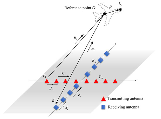
Figure 1.
MIMO radar target 3D imaging geometry.
To get high range resolution and fulfill the requirement of cognitive suppression of WBI, the frequency-stepped narrow-band orthogonal signal is adopted by each transmitting antenna, which can also help to avoid the use of high-speed analog to digital converters. For the q-th frequency (sub-pulse) and the m-th transmitting antenna, the transmitted signal can be expressed as
where , is the signal duration, , , is the number of sub-pulses, is the rectangle function, , is the duration of each sub-pulse, is the q-th frequency, is the starting frequency, is the frequency step, and is the modulation phase of the m-th transmitting antenna.
After being backscattered from the target, the signal received by the n-th receiving antenna can be expressed as
where , is the delay of the p-th scattering center at the q-th sub-pulse with the reference point at (xo + vx(q − 1)Tr, yo + vy(q − 1)Tr, zo + vz(q − 1)Tr), c is the speed of light, and are the distances from the m-th transmitting antenna and the n-th receiving antenna to the p-th scattering center at the q-th sub-pulse, respectively.
Then, corresponding to the m-th transmitting antenna and the n-th receiving antenna, the received signal in (2) can be down-converted by mixing with a reference signal [27], giving
where is the delay of the reference point with respect to the m-th transmitting antenna and the n-th receiving antenna at the q-th sub-pulse (here, it is assumed that the target velocities vx, vy, and vz can be estimated with a high accuracy), , and .
As the transmitted signal in each sub-pulse is narrow-band, the down-converted signal can go through a low-pass filter to suppress the out-band interference and then be digitally sampled by using a relatively low data sampling rate to get with and . Then, matched filtering (MF) based method [28] can be used to reduce the influences of the signal components from other transmitting antennas, giving
where , denotes the auto-correlation function of the modulation phase of the m-th transmitting signal, whose peak is set as one in the following derivation without loss of generality, and .
Since the bandwidth of each sub-pulse is small, all the scattering centers of the target will locate at the same range cell. Hence, by selecting the peak of (4), a 3D signal cube can be obtained, whose m-n-q-th element is given by
In (5), can be approximated by with [27].
where denotes the wavelength, and denote the distances from the reference point O at (xo, yo, zo) to the first transmitting antenna and to the first receiving antenna, and denote the unitary vectors of and .
Therefore, letting denote the center frequency and , (5) can be rewritten as
where and .
It can be observed that the first three exponential terms in (7) are decoupled and form the basis of the 3D Fourier transform (FT), while the last exponential term is space-frequency coupled and makes the process of the 3D signal cube difficult. Fortunately, according to [29], if , the influence of this exponential term on target imaging can be ignored. To make sure become always smaller than , we can simply set its maximum to be smaller than , i.e.,
Since (where B is the signal bandwidth) and (which is obtained by the Nyquist sampling theorem), (8) can be simplified to
Therefore, by setting the system parameters to make the condition in (10) always satisfied, we can get the 3D signal cube used for target imaging in this study, as given in (11).
Based on the signal model given in (11), the target parameters can be simply obtained by using the 3D inverse fast FT (IFFT) or the high-resolution spectral estimation-based method [30]. At last, based on , the target position {x, y, z} = {[x1,…,xp], [y1,…,yp], [z1,…,zp]} can be obtained by solving the set of ternary quadratic equations in (6). For example, as we set et = [1, 0, 0] and er = [0, 1, 0] in the simulations, it can be derived that xp = −αpλcrT/dt and yp = −βpλcrR/dr. Then, zp can be obtained according to the definition of χp.
2.2. WBI Influences
WBI is a generalized term for the interference that occupies a wide frequency band. Since the radio frequency environment becomes more and more crowded, the source of WBI may be complicated, such as the communication/broadcasting signal, the non-cooperative radar signal, the intentional jamming signal, and many others, leading to the complexity of WBI. According to [4,14], the WBI existing in the environment has two typical forms, i.e., chirp-modulated WBI (CM-WBI) and sinusoidal-modulated WBI (SM-WBI). In this study, to reflect its dynamic property, the WBI is modeled by simultaneously considering these two typical WBIs, expressed as
with
where denotes the period of the CM-WBI, and denote the carrier frequencies, denotes the chirp rate, , , and denote the amplitude, frequency, and phase of the g-th () sinusoidal signal of the SM-WBI with G as the number of sinusoids, and denote the modulation amplitudes, modeled as band-passed Gaussian noise signals with standard deviations of and that are determined by the interference-to-signal-ratios (ISRs).
To give an impression about the WBI, Figure 2 shows the time–frequency spectrum (TFS) diagrams of the transmitting signal and the WBI. For the transmitting signal, we set Tw = 7.2 ms, Tr = 0.1 ms, Δf = 2 MHz, Q = 72, and the starting frequency is set as f0 = −71 MHz to make the center frequency 0. For the WBI, we set the ISRs of CW-WBI and SM-WBI as 70 dB, fCM = −40 MHz (i.e., the carrier frequency of CM-WBI is 40 MHz lower than the center frequency of the transmitting signal), μ = 5 MHz/ms, TCM = 4 ms (i.e., the bandwidth of the CM-WBI is about 20 MHz), fSM = 20 MHz (i.e., the carrier frequency of SM-WBI is 20 MHz higher than the center frequency of the transmitting signal), G = 3, β1 = 5 × 10³, φ1 = 0, f1 = 200 Hz, β2 = 7.5 × 10³, φ2 = π/2, f2 = 350 Hz, β3 = 10 × 103, φ3 = π, and f3 = 500 Hz. It can be seen from Figure 2 that the WBI will pollute some frequency bands of the radar signal, thus affecting the process of some sub-pulses. In the following, the influences of WBI on target imaging will be analyzed in detail.
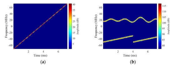
Figure 2.
TFS diagrams of (a) the transmitting signal and (b) the considered WBI with ISR = 70 dB.
For the frequency-stepped narrow-band orthogonal signal used in this paper, its wide bandwidth is obtained by changing the carrier frequencies of the radar signal in different sub-pulses. For each sub-pulse, its instantaneous bandwidth is limited. Hence, the WBI will not pollute the signal frequency band completely in each measurement. In other words, as given in (3), the received signal will be down-converted and then be low-pass filtered, resulting in the fragmentized WBI segments that only affect partial sub-pulses that work in the WBI occupied bands, as illustrated in Figure 3.
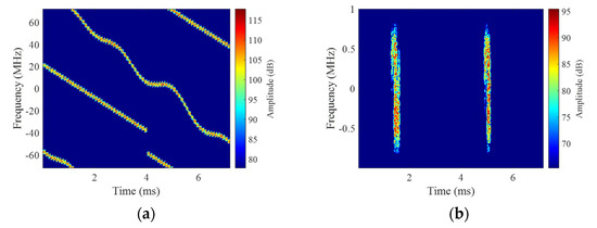
Figure 3.
TFS diagrams of the WBI after (a) down-converting and (b) low-pass filtering with a pass frequency of 0.5 MHz and a stop frequency of 1 MHz.
As a consequence, the MF-based process, as given in (4), will be destroyed only for the sub-pulses that are affected by the WBI segments. As shown in Figure 4, for the non-interfered sub-pulse, the peak of (4) can still be easily identified; thus, the following process can be normally conducted, while, for the interfered sub-pulse, the strong WBI segment will make the MF-based process fail.
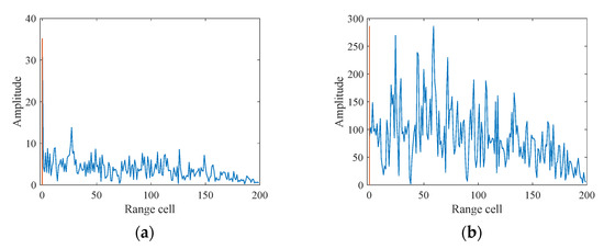
Figure 4.
The MF results of (a) the non-interfered sub-pulse and (b) the interfered sub-pulse.
Therefore, considering the influences of WBI, the 3D signal cube given in (11) should be changed to
where the signal component corresponding to the sub-pulse indexed by will be unusable and is the index set of all the WBI-interfered sub-pulses in the current measurement.
It should be noted that, considering the time-varying property of the WBI, may vary for different measurements with an interval of the signal duration Tw. In such a case, we may need several measurements to obtain the complete information of WBI, i.e., to get a full index set to represent the frequency bands occupied by the WBI and all the sub-pulses that may be affected by the WBI. Hence, in each measurement, should be determined and then combined with those obtained from previous measurements. Besides, (14) also indicates that conventional methods, e.g., 3D IFFT, cannot be directly used for target imaging when WBI exists and thus some advanced methods should be exploited.
2.3. Sparse Sampling (SS)
For MIMO radar applications, SS can be seen as the selection of a sub-dataset from all the available spatial and temporal (frequency) samples. Compared to the full sampling method, SS is able to save radar resources and get similar performance by using some advanced processing methods that exploit the data structure and the target properties (e.g., the target sparsity in the imaging scene). In general, there are many types of SS, e.g., global SS, partially separable SS, and separable SS (SSS) [31]. In this study, SSS is adopted for MIMO radar target 3D imaging due to its lowest sampling cost. In such a case, the 3D signal cube in (11) should be expressed as
where , , , , , and are the sampling index subsets of transmitting antennas, receiving antennas, and sub-pulses, respectively. The sizes of the subsets, i.e., the numbers of samples in different domains, are , , and , respectively.
There are two ways to determine the sampling index subsets, i.e., the RSS method that selects , , and randomly from the full index sets , , and , and the CSS method that obtains , , and from , , and based on the knowledge of the target and the environment with the help of optimization. In general, the CSS method can achieve higher performance than the RSS method. In the following, we will give a brief analysis of this statement and introduce the basic idea of the proposed cognitive imaging method under SS and WBI.
According to (14), in the current measurement, the structure of the 3D signal cube is shown in Figure 5a, where the black blocks denote the unusable signal components interfered by the WBI and the blue ones denote the non-interfered components. In the framework of RSS, the structure of the signal cube given in (15) is shown in Figure 5b, where the interstitial spaces denote the unsampled signal components. It can be seen that the signal cube still includes some unusable blocks interfered by the WBI. If some methods are used to detect and then remove these blocks, we can get a signal cube shown in Figure 5c, where the translucent blocks denote the removed signal components. On the contrary, in the framework of CSS, with the same numbers of selected antennas and sub-pulses, the structure of the 3D signal cube given (15) is shown in Figure 5d. It can be seen that, as the sampling index subsets are determined by exploiting the information of the target and the WBI, provided by previous measurements, the number of unusable signal blocks, i.e., the interfered signal components, is much reduced, leaving only a few unusable blocks caused by the time-varying property of the WBI. Similarly, by detecting and removing these blocks, we can get the signal cube shown in Figure 5e. At last, by exploiting the sparsity of the target, we can use some advanced methods, e.g., the TSL0 algorithm, to process the sparse signal cube and obtain the 3D high-resolution target image, as shown in Figure 5f.
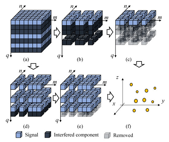
Figure 5.
The schematic diagram that shows the advantage of CSS over RSS and the basic idea of the proposed cognitive sparse imaging method. (a) The structure of the 3D signal cube in (14), (b) the structure of the 3D signal cube in (15) obtained by RSS, (c) the structure of the 3D signal cube obtained by RSS and unusable block removal, (d) the structure of the 3D signal cube in (15) obtained by CSS, (e) the structure of the 3D signal cube obtained by CSS and unusable block removal, and (f) the 3D high-resolution target image obtained by exploiting the target sparsity.
Since the sampling index subsets are more fitted for target imaging and there are more usable signal components, as can be learned by comparing Figure 5c and Figure 5e, the imaging performance of CSS will be higher than RSS if the same imaging method is used. Thus, the proposed cognitive sparse imaging method is mainly realized based on the above-mentioned CSS, WBI-interfered signal component detection and removal (WDR), and 3D high-resolution imaging (HRI), which will be presented in the next Section.
3. Cognitive Sparse Imaging Method
3.1. Cognitive Loop
According to the analysis in Section 2, the proposed imaging method for MIMO radar under SS and WBI is based on a cognitive loop that mainly includes 4 steps, as shown in Figure 6.
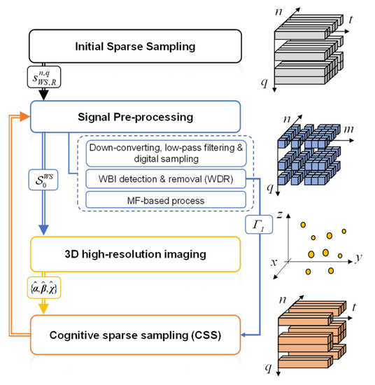
Figure 6.
Flowchart of the proposed cognitive sparse imaging method.
3.1.1. Step 1: Initial Sparse Sampling
In the initial measurement, assuming there is no knowledge of the target and the WBI, in order to reduce the sampling cost, the RSS method will be used to select limited transceiving antennas and sub-pulses for target imaging, giving
where denotes the WBI signal for the q-th sub-pulse and the n-th receiving antenna, , and the subscript WS denotes SS in the presence of WBI. Equation (16) indicates that, when and , the signal will be sampled according to transmitting antennas. Otherwise, no signal will be sampled.
3.1.2. Step 2: Signal Pre-Processing
(1) Down-converting, low-pass filtering, and digital sampling
Corresponding to the mS-th selected transmitting antenna, the nS-th selected receiving antenna, and the qS-th selected sub-pulses, will be down-converted to
where denotes the delay of the reference point. Then, low-pass filtering and digital sampling will be conducted to suppress the out-band WBI and get .
(2) WBI-interfered component detection and removal (WDR)
The signal array includes some components that are interfered by WBI, which should be detected and removed (i.e., set to 0), expressed as
The index set that includes all the detected in the current measurement will be saved into the full WBI index set for the CSS process in the following measurements. In this study, the averaged amplitude (AA) will be used as the indicator for WBI-interfered signal component detection.
(3) MF-based process and peak selection
For , to reduce the influences from other transmitting antennas, MF process will be conducted, giving
By selecting the peak with from (19), we get
which denotes the signal components that will be used for the following process.
3.1.3. Step 3: 3D High-Resolution Imaging (HRI)
After signal pre-processing given in (17)–(20), we can get a 3D signal cube whose m-n-q-th element can be expressed as
Compared to the signal cube given in (11), the signal cube given in (21) cannot be directly applied for target imaging by conventional methods. Hence, we will use the TSL0 algorithm to get the 3D high-resolution image of the target considering the effectiveness and wide application of the SL0 algorithm in radar imaging [2,19,26,28,31], which will also provide target information for the next measurement. In this study, the target information is obtained by extracting the target parameter , where is the number of strong points in the target image whose coefficients are higher than a given threshold.
3.1.4. Step 4: Cognitive Sparse Sampling (CSS)
The CSS can be regarded as a dynamic interaction with the target and the WBI to select the optimal sampling index subsets , , and for the next measurement by exploiting the information provided by and . In general, the target information is exploited to get the best sampling strategy and the WBI information is exploited to avoid the negative influences of the WBI on target imaging. In this study, the CSS will be realized by solving a discrete optimization problem by the greedy algorithm.
After CSS, the signal will be processed based on Step 2 and Step 3 to get the cognitive 3D HRI result of the target, and then CSS will be conducted again for the next measurement. In the following, three main modules of the cognitive loop, i.e., WDR, HRI, and CSS, will be detailed.
3.2. WDR Module
The WDR is the first important module of the cognitive sparse imaging method to provide: (1) the WBI information for the CSS in the following measurements and (2) the useful signal components for the HRI process. It will be conducted based on , a four-dimension signal array, to find the set to indicate the WBI-interfered sub-pulses.
For each pair of transceiving antennas, since the WBI is normally much stronger than the target echoes, the amplitude of data samples in the interfered sub-pulses will be much higher than those in the regular sub-pulses. Therefore, we can get by using a simple indicator, i.e., the AA of the data samples of each sub-pulse, whose mS-nS-qS-th element is defined by
Based on (22), the WBI-interfered sub-pulse can be detected if AA is higher than a threshold, expressed as
where denotes the WBI-interfered sub-pulse index for the mS-th selected transmitting antenna and the nS-th selected receiving antenna. The detection threshold can be set as a fixed value in advance empirically or be determined adaptively by some efficient techniques, e.g., the cell-averaging CFAR (CA-CFAR) technique or the smallest-of CFAR (SO-CFAR) technique [24].
In principle, for different pairs of transceiving antennas, the interfered sub-pulses should be the same, i.e., . Hence, in order to get better detection performance without missing any interfered sub-pulses, we get the sub-pulse index set by
After detection, according to (18), the signal components indexed by should be removed, i.e., set to 0, and should be merged into for CSS, i.e., .
3.3. HRI Module
Based on the CS theory, and considering there are only a few strong scattering centers of the target, we solve the following problem for 3D HRI with the sparse signal cube [26].
where denotes the 3D image of the target, denotes the number of nonzero elements in a tensor, denotes the noise level, ×κ denotes the mode-κ tensor by matrix product, , , , , and denote the under-sampled Fourier transform matrices corresponding to , , and with , , and , where , , and are given by
with , , and as the imaging grid numbers.
Since directly solving (25) is difficult, we use the TSL0 algorithm to solve (25) in this study. Firstly, according to [26], a function is formulated to measure the sparsity of the target image as
where σ is an auxiliary variable and is the m0-n0-q0-th element of .
It is clear that
which indicates that, when σ is close to 0, will approximate the L0 norm of . Therefore, solving (25) is similar to solving the following minimization problem,
For the TSL0 algorithm, (29) is solved iteratively by setting a decreasing sequence of σ and, for each σ, the steepest descent algorithm followed by the projection onto the feasible set is used to get . The details of the TSL0 algorithm are shown in Algorithm 1.
| Algorithms 1 Tensor-based SL0 (TSL0) algorithm |
| Input:, , , , iteration number W and H. Procedure: (1) Initialization: , a suitable decreasing sequence , the step size μ, and w = 1. (2) Let . (3) Minimize the cost function on the feasible set using H iterations of the steepest descent algorithm (followed by the projection onto the feasible set) as shown in the following and then go to (4). (3.1) Initialization ; (3.2) For : (3.2.1) ; (3.2.2) ; (3.2.3) . (4) Set and go to (5). (5) Let . If go back to (2), or else stop. Output: . |
After 3D HRI, the target information will be extracted, giving , , and that satisfy , where is the amplitude threshold that balances the imaging accuracy and the number of selected strong points.
3.4. CSS Module
The aim of CSS is to use the obtained WBI index set and the target parameter as the known information to achieve the optimal selection of given-number transceiving antennas and sub-pulses. Similar to the cognitive antenna selection method used for MIMO radar target 2D imaging [9], with the help of the sub-modularity concept [32], the CSS used in this study is realized by solving a discrete optimization problem whose cost function is defined as the MSE of the target parameter estimated by using only partial transceiving antennas and sub-pulses.
Since MSE is not submodular in general, the frame potential (FP) [22,23] is used as a tight surrogate of the MSE, expressed as
where tr[·] denotes the trace of a matrix, denotes the conjugate transpose process, denotes a Grammian matrix, , is defined by [23]
with denoting the Khatri–Rao product between two matrices, , , , , , , , , and as the row-sampling matrices according to , , and , respectively.
It should be noted that, in (31), the target information is contained in , , and , and the WBI information is exploited by setting (when WBI exists, some of the sub-pulses selected by the CSS method that only considers the target information may be polluted, resulting in performance degradation, and, to solve this problem, a natural idea is to leave the WBI-interfered sub-pulse indexes out when conducting CSS, i.e., setting ).
According to the property of the Khatri–Rao product, the Grammian matrix and the FP can be rewritten as [9]
and
where denotes the Hadamard product between two matrices, , , and denote the Grammian matrices corresponding to the transmitting antennas, receiving antennas, and sub-pulses, respectively.
As indicated in [20], since in (33) is not a monotone non-decreasing, normalized, and submodular set function, it cannot be directly used as the cost function to meet the expected performance guarantee. Hence, the cost function is redefined by modifying to [33]
where is the complement set of that denotes the index sets of non-selected transceiving antennas and sub-pulses, denotes the index set of all available antennas and sub-pulses with the size of , and it should be noted that the WBI information, i.e., , is thus contained in by setting .
Therefore, the proposed CSS method conducted via the minimization of MSE is reformulated as the maximization of , expressed as [23]
where is the truncated partition matroid constraint to ensure as a non-singular matrix with and .
Equation (35) is a submodular discrete optimization problem that can be solved via the convex optimization algorithm [34] or the greedy algorithm [20,21]. Considering its higher efficiency, the greedy algorithm is used in this study, as given in Algorithm 2.
After solving (35), the optimal SS index sets, and thus the corresponding 3D signal cube, can be obtained. Hence, limited transceiving antennas and sub-pulses can be used for HRI with a reduced sampling cost and more radar resources can be reserved for other tasks.
| Algorithms 2 Greedy algorithm |
| Input:, , , , , , , , , and . Procedure: (1) Initialization: , , and . (2) Repetition: (2.1) If stop, or else continue; (2.2) Find the index satisfying: ; (2.3) and . Output: . |
3.5. Complexity Analysis
Without considering down-converting, low-pass filtering, and digital sampling, which are implemented in the data measurement stage, the computing complexity of the proposed cognitive sparse imaging method in each loop mainly comes from WDR, MF, HRI, and CSS (or RSS in the first loop, whose complexity can be ignored).
For WDR, if an empirical threshold is used, the complexity is ignorable, i.e., ; if the CFAR technique is used, the complexity in terms of multiplications is , where denotes the number of reference cells. For MF conducted via FFT and IFFT, the complexity is . For HRI using the TSL0 algorithm shown in Algorithm 1, the complexity of the initialization step is and the complexity of each iteration is . Thus, the complexity of HRI is . For CSS using the greedy algorithm shown in Algorithm 2, the complexity depends on the evaluation of in iterations. According to (32) and (33), the complexity of calculating is , and, in the l-th () iteration, given , , , and with , , and , we need to: (1) evaluate over each transmitting antenna index , giving a complexity of ; (2) evaluate over each receiving antenna index , giving a complexity of ; and (3) evaluate over each sub-pulse index , giving a complexity of . Therefore, the complexity of CSS is .
Based on above analysis, the computing complexity of the proposed cognitive sparse imaging method can be expressed as in the first loop and from the second loop. In general, the HRI has the dominant complexity in the proposed method, higher than other steps. Besides, compared to the sparse imaging method with only RSS, MF, and HRI, the additional complexities and are relatively low.
4. Simulation Results
In this Section, various simulations are conducted to evaluate the proposed cognitive sparse imaging method. First, without SS, we show the influence of WBI on target imaging and the performance of WDR and HRI. Then, we show the advantage of CSS over RSS on target imaging in the absence of WBI. Lastly, we show the performance of the proposed cognitive sparse imaging method considering WBI and SS simultaneously. It should be noted that, to be more practical, all the simulations are conducted based on the received signal modeled in (2) or (16). Therefore, the influences of down-converting, low-pass filtering, and MF-based process on target imaging are included.
Simulation parameters are set as: center frequency fc = 10 GHz, frequency step Δf = 2 MHz, sub-pulse number Q = 72, sub-pulse duration Tr = 0.1 ms, antenna number M = N = 36, antenna spacing dt = dr = 8 m. Transmitting antennas are set along the x-axis and receiving antennas are set along the y-axis. A random polyphase coding method is used to set the modulation phases of different transmitting antennas. The reference point is set as the coordinate origin and its distance to the radar system is set as 10 km at the initial time. The target velocity is set as (150, 150, 0) m/s and there are P = 47 scattering centers whose 3D positions relative to the reference point are shown in Figure 7. Based on (6), the target parameters can be obtained, as shown in Figure 8. In the following, we use Figure 8 as the ground-truth for target imaging without changing back to .
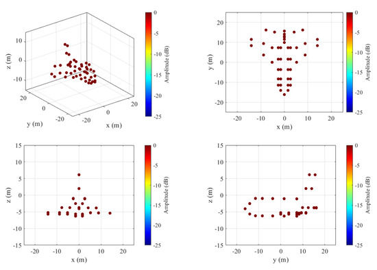
Figure 7.
3D positions of the scattering centers of the simulated target.
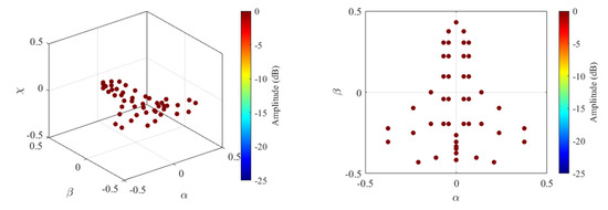
Figure 8.
Ground-truth for simulated target imaging.
With the above system parameters and target model, the feasibility of the approximations used to establish the signal model in this study is first validated. For all sub-pulses, transmitting antennas, receiving antennas, and target-scattering centers, the maximal difference between the phase terms of (5) and (11) is about 0.48 π, smaller than π/2. Moreover, at the lowest frequency f1, highest frequency f72, and close-center frequencies f36 and f37, the maximal phase differences of all target-scattering centers for different transceiving antennas are shown in Figure 9. It can thus be concluded that the signal model given in (11) is reasonable for MIMO radar target 3D imaging.
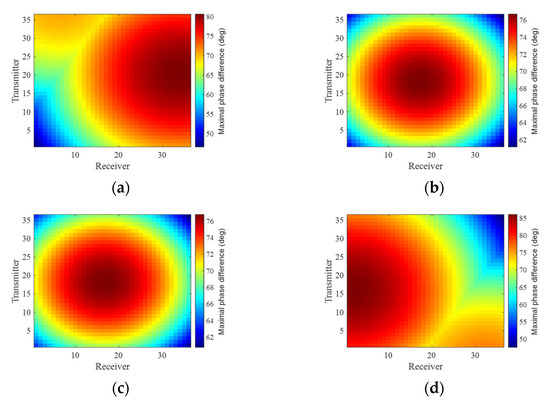
Figure 9.
Maximal phase differences of all target-scattering centers for different transceiving antennas at (a) f1, (b) f36, (c) f37, and (d) f72.
To assess the imaging performance of different methods in different conditions, normalized mean square error (NMSE) and image contrast (IC) are applied to quantitatively evaluate the imaging results. Target image with higher quality will have lower NMSE and higher IC. The two indicators are defined as
where denotes the target image obtained by different methods in the i-th Monte Carlo trial, Ave{·} denotes the averaging operations of all image elements, and I denotes the number of Monte Carlo trials.
4.1. Imaging Results under WBI
For the receiving signal that only contains target echoes, we can perform down-converting, low-pass filtering, digital sampling, and MF to obtain the signal cube as modeled in (5). Then, according to the model in (11), we can simply use the 3D IFFT to get the target image, as shown in Figure 10, where the signal-to-noise ratio (SNR) is set as 0 dB in each sub-pulse. According to (11), the imaging resolutions of the target parameters α, β, and γ obtained by the simple 3D IFFT method are given by , , and . Then, according to (6) and considering the sizes of both the target and the MIMO array are far less than the distance between the MIMO array and the target, the imaging resolutions of the target positions x, y, and z can be derived as , , and . It can be seen from Figure 10 that all the scattering centers of the target are well focused, corresponding to the ground-truth. However, when WBI exists, the target image quality will be seriously degraded, as shown in Figure 11, where the WBI parameters are the same as those used in Figure 2 except that fCM = fc − 40 MHz and fSM = fc + 20 MHz here.
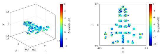
Figure 10.
Target imaging result obtained by the 3D IFFT.
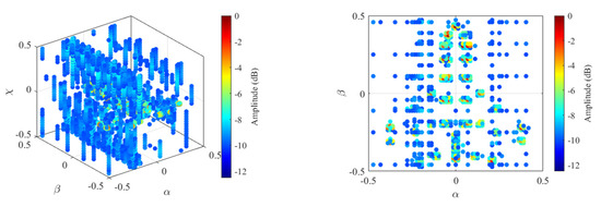
Figure 11.
Target imaging result obtained by the 3D IFFT in the presence of WBI with ISR = 70 dB.
Assuming the WBI parameters are randomly selected in the ranges given in Table 1 and the ISRs of SM-WBI and CM-WBI are equivalent, the NMSEs and ICs of the target images obtained by the 3D IFFT under different ISRs are shown in Figure 12, where 1000 Monte Carlo trials are conducted for each ISR. It can be seen that, with the increase in the ISR, the NMSE becomes higher and the IC becomes lower. Therefore, when the WBI is strong (e.g., the ISR is higher than 50 dB), which is normally the case in practice, some advanced methods should be developed to improve the target imaging performance, i.e., to reduce the negative influence of WBI.

Table 1.
Value range of the WBI parameters.
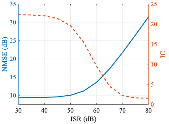
Figure 12.
NMSEs and ICs of the target images obtained by the 3D IFFT under different ISRs with random WBI parameters.
For the proposed cognitive imaging method, WDR is used to provide the WBI information, i.e., to get . As mentioned in Section 3, after performing down-converting, low-pass filtering, and digital sampling on the receiving signal, the AA of the signal array can be used as the indicator to get . With the SNR as 0 dB and the same WBI parameters as Figure 11, for the first transmitting antenna, the AAs corresponding to different sub-pulses and receiving antennas are shown by the red surface in Figure 13. It can be seen that the WBI-interfered sub-pulses are clearly indicated by the AA values. Hence, either based on an empirical threshold or an adaptive threshold, can be easily obtained, as shown in Figure 13, where the SO-CFAR algorithm with a guard cell number of 4, a false alert rate of 10−3, and a reference cell number of 8 is used to determine the detection threshold (i.e., the blue surface).
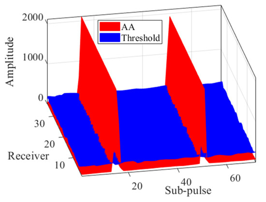
Figure 13.
The AA and detection threshold for the first transmitting antenna with ISR = 70 dB.
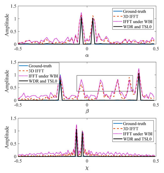
After getting , i.e., after WBI detection, as shown in (18), the WBI-interfered sub-pulses can be removed and the TSL0 algorithm given in Algorithm 1 can be used to get the 3D HRI result, as shown in Figure 14, where, for the TSL0 algorithm, W = 11, H = 3, , , , , and are constructed based on , , and as no SS is applied here. It can be seen that a high-quality target image can be obtained by TSL0 after WDR, giving an NMSE of about −15.37 dB. Besides, the comparisons of Figure 10, Figure 11 and Figure 14 are given in Figure 15, from which it can be seen that the proposed method can obtain higher imaging resolution and lower sidelobe level.
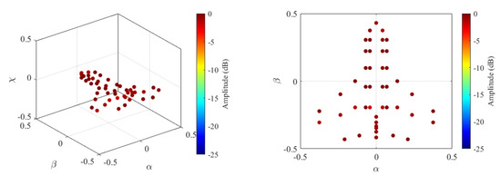
Figure 14.
Target imaging result obtained by TSL0 after WDR with ISR = 70 dB. Compared to Figure 10, the target-scattering centers are more clearly separated, indicating the higher imaging resolution obtained by TSL0 than 3D IFFT.
Similar to Figure 12, with 1000 Monte Carlo trials, the NMSEs and ICs of the target images obtained by TSL0 under different ISRs are shown in Figure 16. It can be seen that, with various ISRs, small NMSEs and high ICs can always be achieved, verifying the imaging performance of the proposed method. It should be mentioned that the slight performance decrease along with the ISR increase is caused by the WBI leakages to all sub-pulses after low-pass filtering.
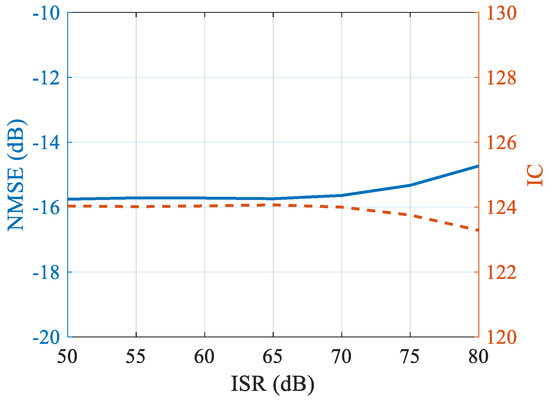
Figure 16.
NMSEs and ICs of the target images obtained by TSL0 after WDR under different ISRs with random WBI parameters.
4.2. Imaging Results under SS
Sparse sampling can help to save radar resources and reduce sampling cost (transceiving antennas and sub-pulses). However, when the signal cube is sparsely sampled, conventional imaging methods cannot be used to obtain a high-quality target image. For example, by using the RSS scheme and setting SNR = 0 dB and , the target image obtained by the zero-padded 3D IFFT is shown in Figure 17, where many high-level artifacts are generated.
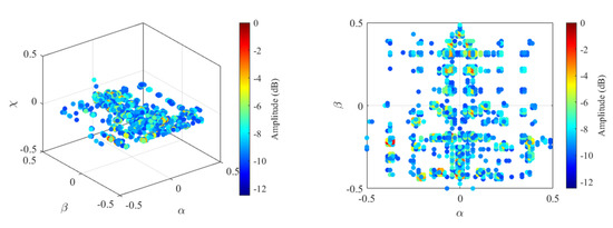
Figure 17.
Target imaging result obtained by the zero-padded 3D IFFT with random sparse-sampled signal cube.
In such a case, we can use the CS-based method to obtain a well-focused target image. By using the TSL0 algorithm, we obtain the 3D HRI result shown in Figure 18 with the same data as Figure 17. Here, is constructed by setting as no WBI is considered. It can be seen from Figure 18 that, even with the sparsely sampled signal, the TSL0 algorithm can still obtain a 3D high-resolution target image, better than that obtained by the zero-padded 3D IFFT.
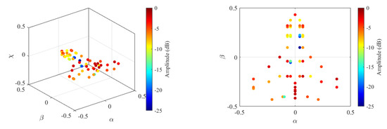
Figure 18.
Target imaging result obtained by TSL0 with random sparse-sampled signal cube.
However, RSS does not exploit the target information for imaging. On the contrary, the CSS method proposed in this study exploits the target information to get higher imaging performance. For example, based on the greedy algorithm shown in Algorithm 2 with (as no WBI is considered here) and , we can obtain the optimal sparse selection of transceiving antennas and sub-pulses, giving the 3D HRI result shown in Figure 19. It can be seen that the image is more focused than Figure 18; the NMSEs of the target images shown in Figure 18 and Figure 19 are −4.93 dB and −9.24 dB, respectively, indicating the superiority of the CSS method.
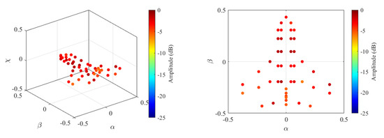
Figure 19.
Target imaging result obtained by TSL0 with cognitive sparse-sampled signal cube.
It should be noted that Figure 18 only shows one imaging example of the RSS method. Considering its randomness, the RSS method can actually obtain higher imaging performance than that shown in Figure 18. In order to fairly compare the RSS method and the CSS method, two additional simulations are conducted.
Firstly, keeping SNR = 0 dB and MS = NS = QS/2, we calculate the NMSEs of the RSS method and the CSS method by changing the number of selected transmitting antennas MS from 16 to 30 with a step of 2. For each MS, 1000 RSSs are conducted and the maximum, minimum, and mean values of the NMSEs are saved. By averaging over 10 Monte Carlo trials, the obtained results are shown in Figure 20.
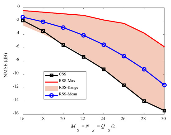
Figure 20.
NMSEs of the RSS method and the CSS method against the number of selected antennas and sub-pulses.
Secondly, keeping MS = NS = QS/2, we calculate the NMSEs of the RSS and CSS methods by changing the SNR from −55 dB to 0 dB with a step of 5 dB. Similarly, for each SNR, 1000 RSSs are conducted. With 10 Monte Carlo trials, the obtained results are shown in Figure 21.
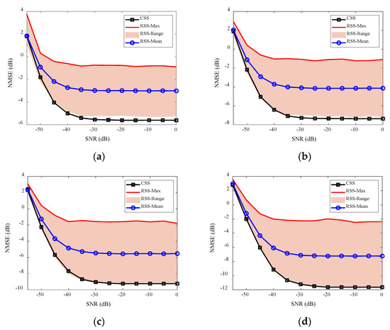
Figure 21.
NMSEs of the RSS method and the CSS method against SNRs with (a) MS = NS = QS/2 = 20, (b) MS = NS = QS/2 = 22, (c) MS = NS = QS/2 = 24, and (d) MS = NS = QS/2 = 26.
4.3. Cognitive Imaging under SS and WBI
In the previous two sub-Sections, we show the performance of WBI detection without SS, HRI by TSL0 with WBI, HRI by TSL0 with SS, and CSS without WBI; i.e., main modules of the proposed cognitive sparse imaging method have been verified separately. In this sub-Section, we show the performance of the cognitive sparse imaging method under SS and WBI at the same time. To verify the proposed method in different loops, we set MS = NS = QS/2 = 24 and the number of measurements (loops) as 10 (i.e., the total measurement duration is 48 ms). For CSS in each loop, the target information is obtained by setting the normalized amplitude threshold as −25 dB, i.e., and the WBI information is obtained by WBI detection and .
Firstly, we show the WBI detection performance of the proposed method under different conditions. Three WBIs are generated, as shown in the left subfigures of Figure 22, where the white vertical lines indicate the starting/ending time of different measurements (i.e., loops). The left-top subfigure of Figure 22 is obtained by using the same WBI parameters as those used for Figure 11, while the WBI parameters for generating left-middle and left-bottom subfigures of Figure 22 are randomly selected in the ranges given in Table 1 with the ISRs of CM-WBI and SM-WBI randomly selected from [50 dB, 80 dB]. It can be seen from the right subfigures of Figure 22 that, under different conditions, the complete WBI information, i.e., the frequency bands occupied by the WBI and the sub-pulses that may be affected by WBI, can be well obtained with the increase in loop number, verifying the WBI detection performance of the proposed method. It should be mentioned that, due to the randomness of the initial SS step in the proposed method (i.e., the randomness in the first loop), Figure 22 only shows some examples of WBI detection and the identified WBI-interfered sub-pulses may become unchanged from various loops.
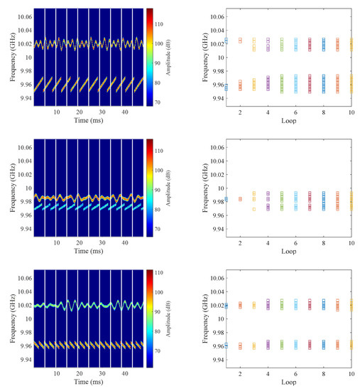
Figure 22.
(Left) TFS diagrams of three WBIs with different parameters and (right) the corresponding WBI-interfered sub-pulse detection examples.
Secondly, we show the imaging performance and running time of the proposed method under SS and WBI by using the same WBI parameters as those used for Figure 22. Figure 23 shows the NMSEs of the target images obtained by the proposed cognitive sparse imaging method at different loops. For comparison purposes, the NMSEs obtained by the RSS method are also shown. Here, 10 Monte Carlo trials are conducted and the averaged value is obtained. For the RSS method, in each loop and each Monte Carlo trial, 1000 RSSs are conducted and the maximal, minimal, and mean NMSEs are obtained. For the initial SS of the proposed method (i.e., the first loop), in each Monte Carlo trial, 1000 RSSs are conducted and the maximal, minimal, and mean NMSEs of different loops are obtained. It can be seen that, apart from the first loop, where RSS is used, the proposed method can always achieve almost-smallest NMSEs from the second loop, indicating its advantage over RSS. It should be explained that, although the complete WBI information can be obtained after several loops, the TSL0 algorithm can always work well when the size of is slightly smaller than ; thus, the proposed method can obtain high imaging performance just from the second loop.
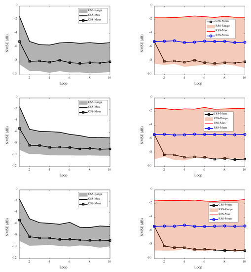
Figure 23.
NMSEs of the proposed cognitive sparse imaging method and the RSS method against the processing loops under three different WBIs.
Figure 24 shows the running time of the proposed cognitive sparse imaging method at different loops. Table 2 shows the running time of different steps of the proposed method at different loops under the first WBI. It can be seen that: (1) as RSS is conducted instead of CSS, the complexity of the first loop is lower than other loops; (2) as CSS starts to be conducted, the complexity of the second loop is the highest; (3) as the size of becomes larger and then unchanged, the running time of the proposed method decreases from the third loop and then becomes stable, which can be derived according to the CSS complexity analysis in Section 3.5; (4) as the WBI bandwidth is widest and thus the size of is generally large, the complexity under the first WBI is lower than those under the other two WBIs, which can be derived according to the MF and HRI complexity analysis in Section 3.5; (5) compared to the running time obtained with only RSS, MF, and HRI, the complexity of the proposed method with additional WDR and CSS does not increase too much, consistent with the analysis in Section 3.5.
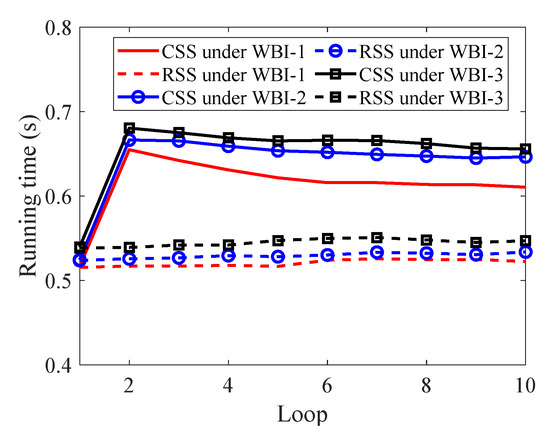
Figure 24.
Running time of the proposed cognitive sparse imaging method and the RSS method against the processing loops under three different WBIs.
Table 2.
Running time of different processing steps of the proposed method at different loops under the first WBI (similar running time can be obtained under the other two WBIs). The unit is ms.
Thirdly, we show the imaging performance of the proposed cognitive sparse imaging method under different ISRs. Given the WBI parameters randomly selected from the ranges in Table 1 and assuming the ISRs of SM-WBI and CM-WBI are equivalent, the NMSEs of the target images obtained by the proposed method and the RSS method at different loops are shown in Figure 25 with different ISRs, where 100 Monte Carlo trials are conducted for each ISR. For the RSS method and the first loop of the proposed method, in each Monte Carlo trial and each ISR, 100 RSSs are conducted and the maximal, minimal, and mean NMSEs are obtained. It can be seen that, under different loops and ISRs, the proposed method can always work well and its performance is higher than the RSS method.
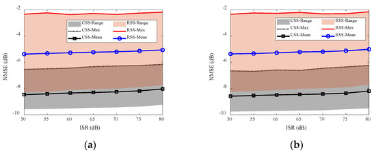
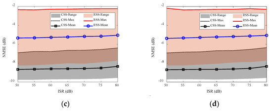
Figure 25.
NMSEs of the proposed cognitive sparse imaging method and the RSS method against ISRs with random WBI parameters at the (a) second loop, (b) fourth loop, (c) sixth loop, and (d) eighth loop.
Finally, similar to Figure 12 and Figure 16, the NMSEs and ICs of the target images obtained at the different loops of the proposed method under different ISRs are shown in Figure 26. It can be seen that, with various ISRs, small NMSEs and high ICs can always be achieved, verifying the imaging performance of the proposed method under SS and WBI at the same time.
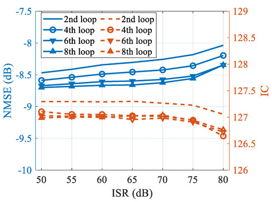
Figure 26.
NMSEs and ICs of the target images obtained at the different loops of the proposed method under different ISRs with random WBI parameters.
5. Experiment Results
To assess the performance of the proposed method in practice, a field experiment was conducted by a software-defined radio (SDR)-implemented 8 × 8 MIMO radar system, as shown in Figure 27. In the imaging scene, several strong reflections exist, e.g., a trihedral corner reflector (CR) and multiple concrete walls, acting as point targets, as indicated by the three red rectangles in Figure 27. Stepped frequency continuous waveform is employed by the SDR-MIMO radar system with the center frequency of fc = 5 GHz, the frequency step selected as Δf = 2 MHz, and the frequency number selected as Q = 72. To guarantee the waveform orthogonality, two 1×8 switches are used to realize the time-divided signal transceiving. More details of the SDR-MIMO radar system and the field experiment can be found in [35].
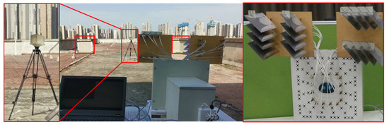
Figure 27.
SDR-MIMO radar experiment setup. The left image shows the trihedral CR and the right image shows the front side of the radar system and the array geometry.
The array structure and the imaging geometry of the SDR-MIMO radar system are shown in Figure 28. Assuming the p-th () target is located at with a scattering coefficient of , for the mr-th transmitter (), the nr-th receiver (), and the q-th frequency (), the signal obtained after data pre-processing (e.g., transceiving antenna direct coupling signal suppression, which is significant for the use of time-continuous waveform for target imaging in practice [35]) can be expressed as
where ,,.
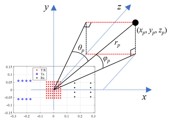
Figure 28.
SDR-MIMO radar array structure and imaging geometry.
To mimic the MIMO radar considered in this paper for target imaging under WBI, the pre-processed signal shown in (38) is phase modulated, giving
The simulated WBI signal can thus be added to the signal in (39) to validate the proposed methods in the presence of WBI and, via the MF method given in (4) and (5), (39) can be transformed back to (38) for imaging process. Besides, as the SDR-MIMO array is designed to be equivalent to a uniform planar array (UPA), as shown by the red crosses in Figure 28, the signal given in (38) can be approximated as
where , , , , , and .
According to the first-order Taylor expansion [7], (40) can be approximated as
where and denote the angles of the p-th target, , , and . With similar approximations as those used to get (11), we can get the following 3D signal model
where , , , and .
It can be seen that the signal model (42) of the SDR-MIMO radar system is similar to that in (11). Thus, the conducted field experiment can be used to validate the proposed methods in this study. Via the back projection (BP) algorithm [35,36], the target image in the x-y-z domain obtained without the approximations in (40)–(42) is shown in Figure 29. It can be seen that the CR and the concrete walls can be well focused, as indicated by the red rectangles in the right sub-figure. Via the 3D IFFT, the target image in the α-β-χ domain obtained based on (42) and its corresponding image in the x-y-z domain are shown in Figure 30. The consistency between Figure 29 and Figure 30 well validates the approximations in (40)–(42). It should be mentioned that, similar to the simulations, the imaging resolutions of the target parameters α, β, and γ obtained by the 3D IFFT are expressed as , , and . Then, according to definitions of , , and , the imaging resolutions of the target position xp, yp, and rp can be derived as , , and .
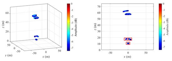
Figure 29.
Real target imaging result obtained by the BP algorithm. The CR and the two close concrete walls are marked by the rectangles in the right sub-figure. The other two scatters indicate two concrete walls further from the radar system.
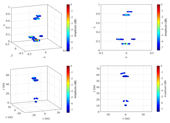
Figure 30.
Real target imaging results obtained by the 3D IFFT in (top) the α-β-χ domain and (bottom) the x-y-z domain.
Given W = 15 and H = 5, the imaging result obtained by the TSL0 algorithm is shown in Figure 31. It can be seen that a high-quality target image with a higher imaging resolution and a lower sidelobe level can be obtained. The targets shown in Figure 31 can be more easily distinguished than those given in Figure 30. Hence, in the following, Figure 31 is used as the ground-truth to assess different results.
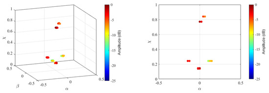
Figure 31.
Real target imaging result obtained by the TSL0 algorithm.
Adding the simulated WBI used for Figure 11 and Figure 14 to the pre-processed signal in (39), the target imaging results obtained by 3D IFFT and TSL0 after WDR are shown in Figure 32. Besides, similar to Figure 12 and Figure 16, with 1000 Monte Carlo trials, the NMSEs (with respect to the result given in Figure 31) and ICs of the target images obtained by TSL0 after WDR under different ISRs are shown in Figure 33. High quality of the bottom sub-figure of Figure 32, low NMSEs, and high ICs indicate the performance of the proposed method under WBI in practice.
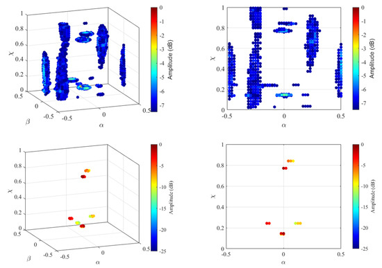
Figure 32.
Real target imaging results obtained by (top) 3D IFFT and (bottom) TSL0 after WDR with ISR = 70 dB.
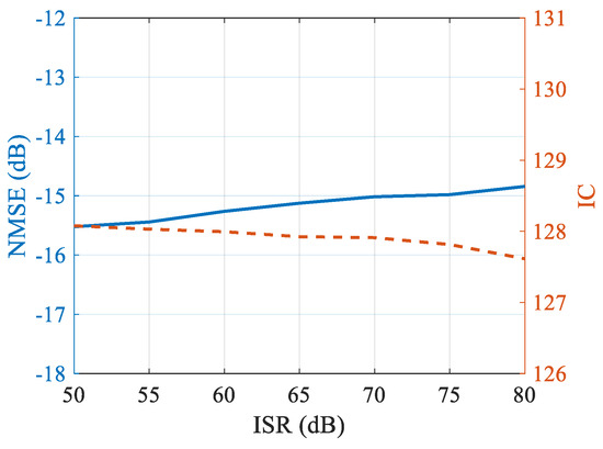
Figure 33.
NMSEs and ICs of the real target images obtained by TSL0 after WDR under different ISRs with random WBI parameters.
Given , , and the target parameter obtained from Figure 31 with the normalized amplitude threshold as −25 dB, the target images obtained by TSL0 under RSS and CSS are shown in Figure 34. Besides, keeping , the NMSEs of the obtained target images under RSS and CSS with the number of the selected frequencies QS changing from 40 to 60 with a step of 2 is shown in Figure 35. Higher quality of the bottom subfigure of Figure 34 and smaller NMSEs in Figure 35 validate the advantage of the proposed cognitive imaging method in practice.
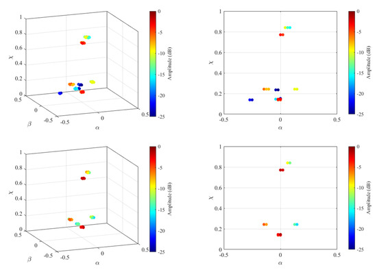
Figure 34.
Real target imaging results obtained by the TSL0 algorithm with (top) random sparse-sampled signal cube and (bottom) cognitive sparse-sampled signal cube.
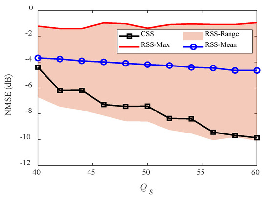
Figure 35.
NMSEs of the real target images obtained under RSS and CSS against the numbers of selected frequencies (sub-pulses).
Lastly, given and , the NMSEs of the target images obtained by the proposed cognitive sparse imaging method and the RSS method in different loops under the three different WBIs shown in Figure 22 are presented in Figure 36. It can be seen that, under WBI and SS simultaneously, the proposed method can always achieve a higher imaging performance in practice.
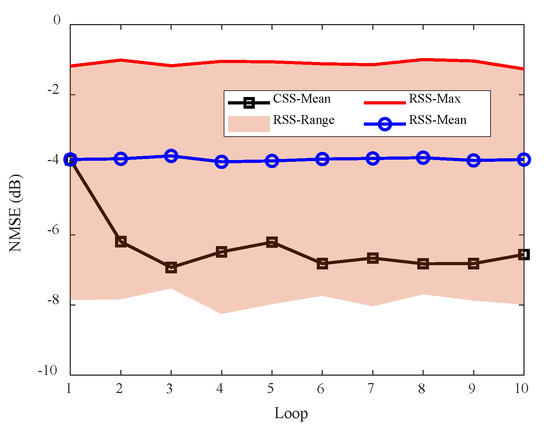
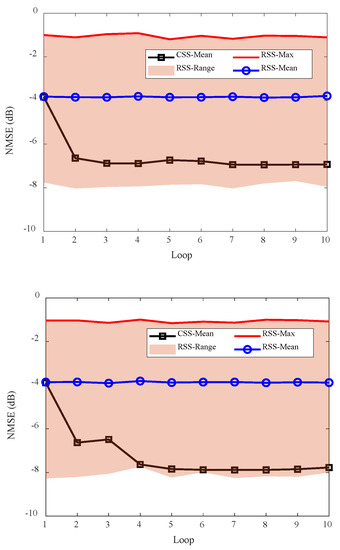
Figure 36.
NMSEs of the real target images obtained by the proposed cognitive sparse imaging method and the RSS method against the processing loops under three different WBIs.
6. Conclusions
In this paper, to reduce the sampling burden and the negative influence of WBI at the same time, a cognitive method was proposed for target 3D high-resolution imaging by a collocated wideband MIMO radar system using a frequency-stepped narrow-band orthogonal signal and the sparse sampling approach. In the proposed method, the WBI information was obtained by the WDR process via the CFAR technique and the target information was obtained by the HRI process via the TSL0 algorithm. By solving an optimization problem, the information of the target and WBI was exploited by the CSS process to obtain optimal selection of transceiving antennas and sub-pulses (frequencies) for target imaging and WBI influence reduction. Simulation and experiment results showed that, under different SS, SNR, and ISR conditions, higher imaging performance can always be achieved by the proposed method than the commonly used RSS method.
Author Contributions
Conceptualization, W.F.; methodology, W.F. and P.W.; software, W.F. and P.W.; validation, W.F., P.W., X.H., Y.G. and H.Z.; writing—original draft preparation, W.F. and P.W.; writing—review and editing, X.H., Y.G. and H.Z.; funding acquisition, W.F. All authors have read and agreed to the published version of the manuscript.
Funding
This work was supported in part by National Natural Science Foundation of China, No. 62001507; China Postdoctoral Science Foundation, No. 2021MD703951; Young Talent fund of University Association for Science and Technology in Shaanxi, China, No. 20210106; and Youth Talent Lifting Project of the China Association for Science and Technology, No. 2021-JCJQ-QT-018.
Data Availability Statement
The data presented in this study are available on request from the corresponding author.
Conflicts of Interest
The authors declare no conflict of interest.
References
- Duan, G.; Wang, D.; Ma, X.; Su, Y. Three-dimensional imaging via wideband MIMO radar system. IEEE Geosci. Remote Sens. Lett. 2010, 7, 445–449. [Google Scholar] [CrossRef]
- Hu, X.; Tong, N.; Guo, Y.; Ding, S. MIMO radar 3-D imaging based on multi-dimensional sparse recovery and signal support prior information. IEEE Sens. J. 2018, 18, 3152–3162. [Google Scholar] [CrossRef]
- Nguyen, L.H.; Tran, T.D. Efficient and robust RFI extraction via sparse recovery. IEEE J. Sel. Top. Appl. Earth Obs. Remote Sens. 2016, 9, 2104–2117. [Google Scholar] [CrossRef]
- Tao, M.; Su, J.; Huang, Y.; Wang, L. Mitigation of radio frequency interference in synthetic aperture radar data: Current status and future trends. Remote Sens. 2019, 11, 2438. [Google Scholar] [CrossRef]
- Rossi, M.; Haimovich, A.M.; Eldar, Y.C. Spatial compressive sensing for MIMO radar. IEEE Trans. Signal Process. 2013, 62, 419–430. [Google Scholar] [CrossRef]
- Hu, X.; Tong, N.; Wang, J.; Ding, S.; Zhao, X. Matrix completion-based MIMO radar imaging with sparse planar array. Signal Process. 2017, 131, 49–57. [Google Scholar] [CrossRef]
- Feng, W.; Friedt, J.-M.; Nico, G.; Sato, M. 3-D ground-based imaging radar based on C-band cross-MIMO array and tensor compressive sensing. IEEE Geosci. Remote Sens. Lett. 2019, 16, 1585–1589. [Google Scholar] [CrossRef]
- Cohen, D.; Eldar, Y.C.; Haimovich, A.M. SUMMeR: Sub-Nyquist MIMO radar. IEEE Trans. Signal Process. 2018, 66, 4315–4330. [Google Scholar] [CrossRef]
- Ding, S.; Tong, N.; Zhang, Y.; Hu, X.; Zhao, X. Cognitive antenna selection in MIMO imaging radar. IEEE Trans. Geosci. Remote Sens. 2021, 59, 9829–9841. [Google Scholar] [CrossRef]
- Mishra, K.V.; Eldar, Y.C.; Shoshan, E.; Namer, M.; Meltsin, M. A cognitive sub-Nyquist MIMO radar prototype. IEEE Trans. Aerosp. Electron. Syst. 2020, 56, 937–955. [Google Scholar] [CrossRef]
- Huang, Y.; Chen, Z.; Wen, C.; Li, J.; Xia, X.; Hong, W. An efficient radio frequency interference mitigation algorithm in real synthetic aperture radar data. IEEE Trans. Geosci. Remote Sens. 2022, 60, 5224912. [Google Scholar] [CrossRef]
- Yang, Z.; Du, W.; Liu, Z.; Liao, G. WBI suppression for SAR using iterative adaptive method. IEEE J. Sel. Top. Appl. Earth Obs. Remote Sens. 2016, 9, 1008–1014. [Google Scholar] [CrossRef]
- Huang, Y.; Zhang, L.; Li, J.; Hong, W.; Nehorai, A. A novel tensor technique for simultaneous narrowband and wideband interference suppression on single-channel SAR system. IEEE Trans. Geosci. Remote Sens. 2019, 57, 9575–9588. [Google Scholar] [CrossRef]
- Huang, Y.; Zhang, L.; Li, J.; Chen, Z.; Yang, X. Reweighted tensor factorization method for SAR narrowband and wideband interference mitigation using smoothing multiview tensor model. IEEE Trans. Geosci. Remote Sens. 2020, 58, 3298–3313. [Google Scholar] [CrossRef]
- Ding, Y.; Fan, W.; Tao, M.; Zhang, Z.; Wang, L.; Zhou, F.; Lu, B. Wideband interference mitigation for synthetic aperture radar based on the variational Bayesian method. Signal Process. 2022, 198, 108581. [Google Scholar] [CrossRef]
- Kirk, B.H.; Narayanan, R.M.; Gallagher, K.A.; Martone, A.F.; Sherbondy, K.D. Avoidance of time-varying radio frequency interference with software-defined cognitive radar. IEEE Trans. Aerosp. Electron. Syst. 2019, 55, 1090–1107. [Google Scholar] [CrossRef]
- Huang, T.; Liu, Y.; Meng, H.; Wang, X. Cognitive random stepped frequency radar with sparse recovery. IEEE Trans. Aerosp. Electron. Syst. 2014, 50, 858–870. [Google Scholar] [CrossRef]
- Pu, T.; Tong, N.; Feng, W.; Wan, P.; Hu, X. MIMO radar sparse recovery imaging with wideband interference prediction. Remote Sens. 2022, 14, 3774. [Google Scholar] [CrossRef]
- Wan, P.; Feng, W.; Tong, N.; Hu, X.; Zheng, G. Wideband interference time–frequency feature prediction and its application to cognitive radar HRRP estimation. IEEE Geosci. Remote Sens. Lett. 2022, 19, 4025105. [Google Scholar] [CrossRef]
- Nemhauser, G.; Wolsey, L.; Fisher, M. An analysis of approximations for maximizing submodular set functions-I. Mathematical programming 1978, 14, 265–294. [Google Scholar] [CrossRef]
- Shamaiah, M.; Banerjee, S.; Vikalo, H. Greedy sensor selection: Leveraging submodularity. In Proceedings of the 49th IEEE Conference on Decision and Control (CDC), Atlanta, GA, USA, 15–17 December 2010. [Google Scholar]
- Kovacevic, J.; Chebira, A. Life beyond bases: The advent of frames (Part I). IEEE Signal Process. Mag. 2007, 24, 86–104. [Google Scholar] [CrossRef]
- Ortiz-Jiménez, G.; Coutino, M.; Chepuri, S.P.; Leus, G. Sparse sampling for inverse problems with tensors. IEEE Trans. Signal Processing 2019, 67, 3272–3286. [Google Scholar] [CrossRef]
- Trunk, G.V. Range resolution of targets using automatic detectors. IEEE Trans. Aerosp. Electron. Syst. 1978, 14, 750–755. [Google Scholar] [CrossRef]
- Qiu, W.; Zhou, J.; Zhao, H.; Fu, Q. Fast sparse reconstruction algorithm for multidimensional signals. Electron. Lett. 2014, 50, 1583–1585. [Google Scholar] [CrossRef]
- Qiu, W.; Zhou, J.; Zhao, H.; Fu, Q. Three-dimensional sparse turntable microwave imaging based on compressive sensing. IEEE Geosci. Remote Sens. Lett. 2015, 12, 826–830. [Google Scholar] [CrossRef]
- Ding, S.; Tong, N.; Zhang, Y.; Hu, X.; Zhao, X. Cognitive MIMO imaging radar based on Doppler filtering waveform separation. IEEE Trans. Geosci. Remote Sens. 2020, 58, 6929–6944. [Google Scholar] [CrossRef]
- Hu, X.; Feng, C.; Wang, Y.; Guo, Y. Adaptive waveform optimization for MIMO radar imaging based on sparse recovery. IEEE Trans. Geosci. Remote Sens. 2020, 58, 2898–2914. [Google Scholar] [CrossRef]
- Han, K.; Wang, Y.; Chang, X.; Tan, W.; Hong, W. Generalized pseudopolar format algorithm for radar imaging with highly suboptimal aperture length. Sci. China Inf. Sci. 2015, 58, 1–5. [Google Scholar] [CrossRef]
- Ding, S.; Tong, N.; Feng, W.; Wan, P.; Zhang, Y. Three-dimensional decoupling imaging method for wideband two-dimensional multiple-input-multiple-output radar. IET Radar Sonar Navig. 2022, 16, 399–411. [Google Scholar] [CrossRef]
- Qiu, W.; Zhou, J.; Fu, Q. Tensor representation for three-dimensional radar target imaging with sparsely sampled data. IEEE Trans. Comput. Imaging 2020, 6, 263–275. [Google Scholar] [CrossRef]
- Das, A.; Kempe, D. Submodular meets spectral: Greedy algorithms for subset selection, sparse approximation and dictionary selection. In Proceedings of the 28th International Conference on International Conference on Machine Learning, Bellevue, WA, USA, 28 June–2 July 2011. [Google Scholar]
- Ranieri, J.; Chebira, A.; Vetterli, M. Near-optimal sensor placement for linear inverse problems. IEEE Trans. Signal Process. 2014, 62, 1135–1146. [Google Scholar] [CrossRef]
- Joshi, S.; Boyd, S. Sensor selection via convex optimization. IEEE Trans. Signal Process. 2009, 57, 451–462. [Google Scholar] [CrossRef]
- Feng, W.; Friedt, J.-M.; Wan, P. SDR-implemented ground-based interferometric radar for displacement measurement. IEEE Trans. Instrum. Meas. 2021, 70, 8502218. [Google Scholar] [CrossRef]
- Feng, W.; Friedt, J.-M.; Nico, G.; Wang, S.; Martin, G.; Sato, M. Passive bistatic ground-based synthetic aperture radar: Concept, system, and experiment results. Remote Sens. 2019, 11, 1753. [Google Scholar] [CrossRef]


Publisher’s Note: MDPI stays neutral with regard to jurisdictional claims in published maps and institutional affiliations. |
© 2022 by the authors. Licensee MDPI, Basel, Switzerland. This article is an open access article distributed under the terms and conditions of the Creative Commons Attribution (CC BY) license (https://creativecommons.org/licenses/by/4.0/).