Article

Topographic Analysis of Intertidal Polychaete Reefs (Sabellaria alveolata) at a Very High Spatial Resolution

1
Institut des Substances et Organismes de la Mer (ISOMer), UR 2160, Nantes Université, F-44000 Nantes, France
2
Société Sciences naturelles de l’Ouest de la France, Nantes, 12 rue Voltaire, F-44000 Nantes, France
3
IFREMER, DYNECO LEBCO, Centre de Bretagne, F-29280 Plouzané, France
*
Author to whom correspondence should be addressed.
Remote Sens. 2022, 14(2), 307; https://doi.org/10.3390/rs14020307
Submission received: 26 November 2021 / Revised: 2 January 2022 / Accepted: 7 January 2022 / Published: 10 January 2022
(This article belongs to the Section Ecological Remote Sensing)

Abstract

:
In temperate coastal regions of Western Europe, the polychaete Sabellaria alveolata (Linné) builds large intertidal reefs of several hectares on soft-bottom substrates. These reefs are protected by the European Habitat Directive EEC/92/43 under the status of biogenic structures hosting a high biodiversity and providing ecological functions such as protection against coastal erosion. As an alternative to time-consuming field campaigns, a UAV-based Structure-from-Motion photogrammetric survey was carried out in October 2020 over Noirmoutier Island (France) where the second-largest known European reef is located in a tidal delta. A DJI Phantom 4 Multispectral UAV provided a topographic dataset at very high resolutions of 5 cm/pixel for the Digital Surface Model (DSM) and 2.63 cm/pixel for the multispectral orthomosaic images. The reef footprint was mapped using a combination of two topographic indices: the Topographic Openness Index and the Topographic Position Index. The reef structures covered an area of 8.15 ha, with 89% corresponding to the main reef composed of connected and continuous biogenic structures, 7.6% of large isolated structures (<60 m2), and 4.4% of small isolated reef clumps (<2 m2). To further describe the topographic complexity of the reef, the Geomorphon landform classification was used. The spatial distribution of tabular platforms considered as a healthy stage of the reef in contrast to a degraded stage was mapped with a proxy that consists in comparing the reef volume to a theoretical tabular-shaped reef volume. Epibionts colonizing the reef (macroalgae, mussels, and oysters) were also mapped by combining multispectral indices such as the Normalised Difference Vegetation Index and simple band ratios with topographic indices. A confusion matrix showed that macroalgae and mussels were satisfactorily identified but that oysters could not be detected by an automated procedure due to their spectral complexity. The topographic indices used in this work should now be further exploited to propose a health index for these large intertidal reefs.

1. Introduction

The honeycomb worm Sabellaria alveolata (Linné) is a gregarious tubiculous reef-building polychaete, inhabiting mostly the intertidal zone of the European coast [1]. It is distributed from Southwest Scotland to North Africa (see the recent updated database from [2]) but also occurs on the Mediterranean coast in closed subtidal environments [3,4]. It is protected under the EU Habitat Directive because it engineers biogenic structures (sheets, veneers, hummocks—see terminology in Curd et al., 2019), which provide habitat for numerous other species throughout its geographic range [5]. The largest intertidal reefs, covering hundreds of hectares from mid to low tide levels, are found in France in the bay of Mont-Saint-Michel (48°40N, 01°40W; [6,7]) and Noirmoutier Island (47°00N, 02°10W; [8,9]). Sabellaria alveolata captures and cements sand particles [10,11] to build a tube joined to those of conspecific adults, resulting in biogenic structures aggregating up to 60,000 individuals per square meter [6,12]. The resulting bioconstructions form complex three dimensional structures with significant ecological functions that interplay with geomorphological processes [7,13]. For example, biogenic structures protect coasts from erosion by wave action [14], while acting as physical barriers and storing large amounts of bioclastic sediment [15]. Their complex 3D structures create a specific habitat, compared to the surrounding substrates, that hosts a high species richness and unique species assemblages [6,16,17,18,19]. Like other types of biogenic reefs created by tube-building polychaetes, they increase the abundance and diversity of sessile and vagile organisms and are considered hotspots of biodiversity [7,20]. Bioconstructions are, however, adversely affected by anthropogenic impacts, some of which are direct, such as mechanical damage by trampling and bivalve hand-fishing inside the reef [21], others indirect as in the case of aquaculture structures that break down currents and sand resuspension [22] or dredging activities that modify the sediment dynamic [9]. Natural extreme events such as excessively cold temperatures and winter storms are also reported to have negative impacts [23].
The protected status of biogenic constructions stipulated by the European Habitat Directive EEC/92/43 implies that changes in habitat surfaces must be monitored and documented, in order to provide guidelines for future conservation strategies. Traditional field measurements undertaken on foot to monitor reef cover and associated epibionts are time-consuming and can be damaging to the reef environment [13]. They require heavy and often costly human power to cover large intertidal reefs, with little replicability in the method and a very low frequency in data acquisition. To overcome these constraints, various remote sensing techniques have been developed to monitor honeycomb worm reef habitats. Earth Observation (EO) with satellites are key tools to map habitat diversity in general, and coastal habitats in particular [24]. They can provide a decametric to metric spatial resolution for commercial products, while publicly available EO data like Sentinel 2 has a 10 m pixel resolution. Yet, they have rarely been used to map intertidal reef habitats [25], as the resolution is often too coarse to describe sub-meter reef features or simply because satellite overpass does not coincide with the lowest tides. Airborne campaigns with multi- or hyper-spectral sensors and topographic/bathymetric LiDAR, as well as underwater sounder dedicated to shallow water, can overcome these tidal restrictions and provide relevant high spatial and spectral resolutions for biogenic reef mapping [22,26,27,28,29]. However, the costs of instrumentation and deployment may limit their use by public environmental agencies. As a result, commercially available unoccupied aerial systems or vehicles (UAVs) have been increasingly used to map intertidal habitats [30,31,32,33,34]. In intertidal soft-sedimentary environments, UAVs destined for the general public have been successfully used to map extensive reefs and associated sedimentary features that are determined using RGB [35] or multispectral cameras [36,37]. UAVs have proven to be a cost-effective technique, enabling repeated surveys for mapping of biogenic reefs. In the race to best characterize and track all fine-scale 3D processes occurring in dynamic habitats such as biogenic formations [38], structure-for-motion (SfM) photogrammetry [35] is an essential tool. However, topographic analysis has not been applied frequently to entire intertidal reefs, with notable exception of [39], even though topographic metrics have been successfully applied to small-scale (meter) reef hummocks [40]. Metrics based on landform analysis [41,42,43,44] could be useful in quantifying reef topographic complexity, which is influenced by reef health and dynamic status.
The main objectives of this study are to (1) apply landform analysis to describe the complex three-dimensional structures of intertidal Sabellaria alveolata reefs using very high-resolution RGB images obtained with a drone equipped with a GPS-RTK positioning system, and (2) map epibionts adversely affecting reef dynamics using a simple workflow based on multispectral images. We used an affordable off-the-shelf UAV for coastal managers to carry out topographic mapping of the reef structure based on the coupling of SfM photogrammetry and visible near infrared imagery. We discussed limitations due to the spectral resolution of the multispectral camera, and used SfM techniques to derive new variables and indices that can be relevant to describe the health status of large intertidal reefs, and further help stakeholders in managing these protected habitats.

2. Materials and Methods
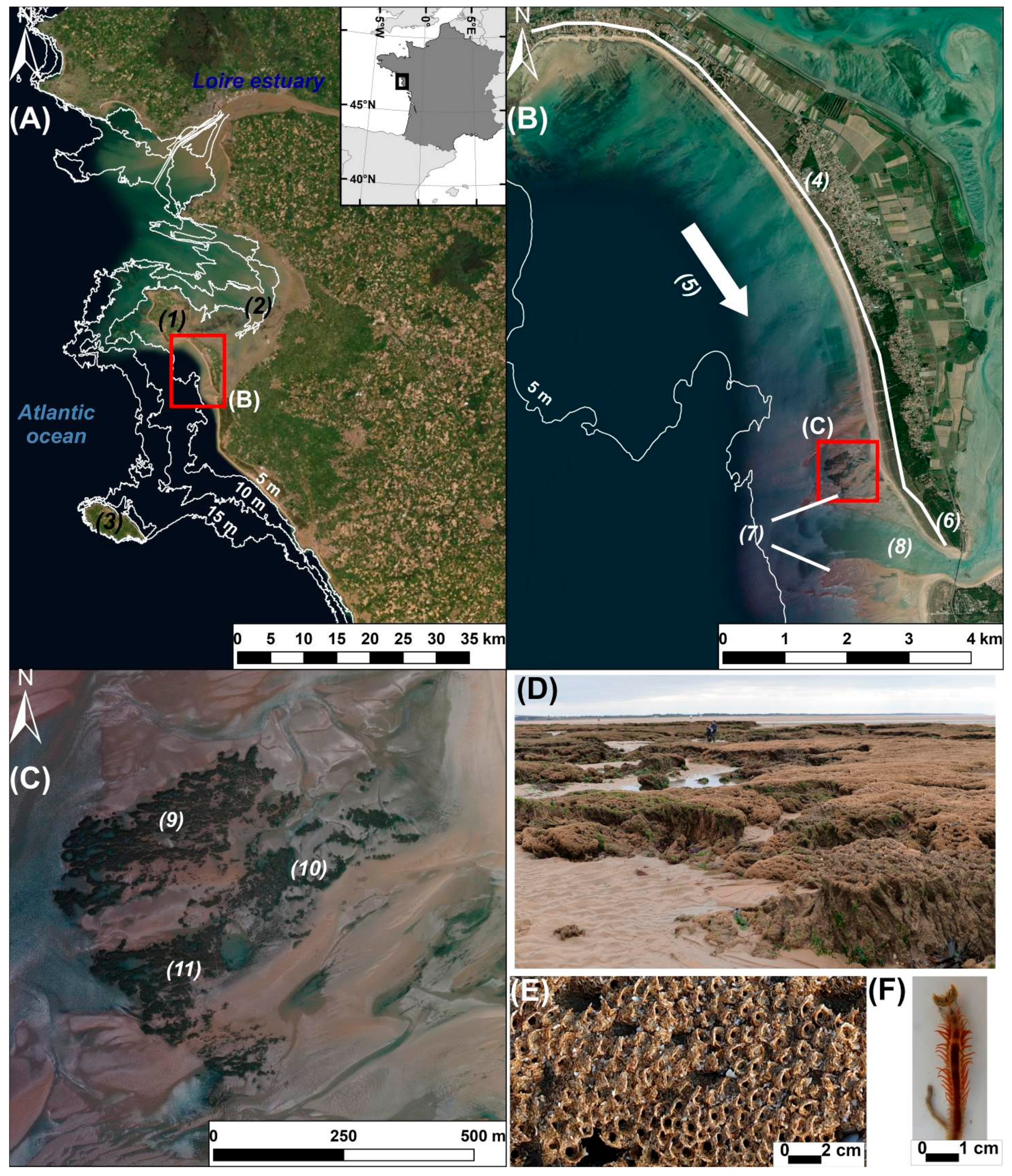
2.1. Study Area

The study area is located on the French Atlantic coast south of Noirmoutier Island (2.25°W, 47°N) in a tidal delta (Figure 1). It covers the second largest intertidal honeycomb worm reef (Sabellaria alveolata) in Europe. This area is part of the NATURA 2000 network designed to cover most ecologically valuable and threatened habitats (Natura 2000 reference: FR5212009) [45]. The honeycomb worm reef thrives on soft sediments and is part of a complex mosaic of coastal habitats that include a beach profile with a large dissipative intertidal platform and a reflective upper beach with a well-developed dune system in the backshore. South of the reef, a sand spit is developing across a large tidal channel, the Goulet of Fromentine [46] connected to a muddier and highly turbid environment, Bourgneuf Bay [47]. The sediment drift is directed southward against the tidal channel. Ebb currents have formed an ebb delta with large swash platforms on each lateral side of the tidal channel [48]. The ebb delta swash platforms and the overall sedimentary and hydrodynamic features provide a favorable environment for reef dynamics. The reef develops on a sandy substrate and is composed of hummocks and platform-type structures, either in progradation (development) or in retrogradation (degradation) phases [1]. Progradation and retrogradation phases are defined based on the structure of the tubes, the presence of epibionts, and the color of the reef compared to the surrounding sediment [1]. From a topographic perspective, the reef shows rounded, tabular, collapsed or incised landforms with heights ranging from decimeters to a meter. The main epibionts colonizing the reef are green macroalgae (Ulva spp.), Pacific oysters (Crassostrea gigas), and blue mussels (Mytilus edulis).

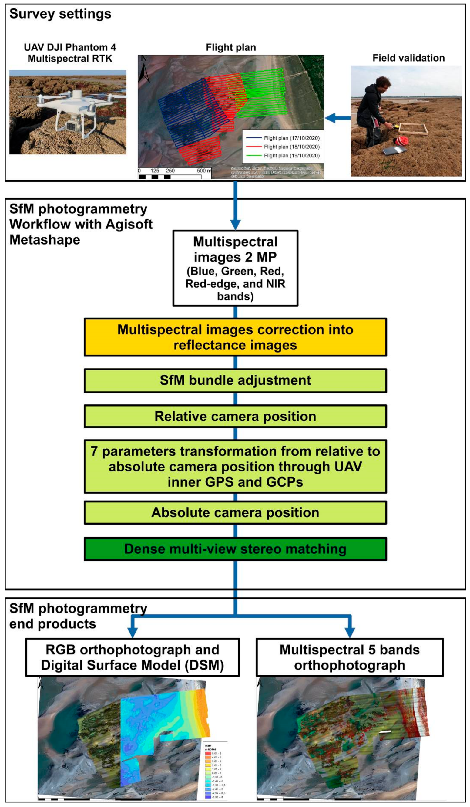
2.2. Survey Settings

The study area was surveyed using an UAV during low tide conditions (17–19 October 2020). The flights were conducted 1 h before low tide around noon to observe the ebb delta and the fully emerged honeycomb worm reef. The images were obtained from a multispectral camera loaded into a DJI Phantom 4 Multispectral with a RTK GPS positioning system (Figure A1). The DJI Phantom 4 Multispectral camera is a global shutter sensor of six separate lenses and CMOS comprising five spectral bands and one RGB sensor at 2.12 MP resolution. It was provided with a 5.27 mm fixed focal lens (equivalent in 35 mm format to a 40 mm focal lens), mounted on gimbals stabilized on 3 axes. The multispectral bands are monochrome sensors with a spectral range including blue (450 nm +/− 16 nm), green (560 nm +/− 16 nm), red (650 +/− 16 nm), red edge (730 nm +/− 16 nm), and near infrared (840 nm +/− 26 nm) wavelengths. The camera system includes a sun incident light sensor on the top of the UAV that is combined with the UAV’s internal GPS receivers (Figure A1). The flight plans were designed using the DJI Ground Station Professional application and by taking account of the specificities of the multispectral camera (Figure A1). As this study aimed to generate a very high-resolution multispectral orthorectified dataset, the Ground Size Dimension (GSD) image pixel was set at 2.6 cm. This implied a flight height of 50 m above ground level over an area of 750 m long-shore × 1000 m cross-shore. The camera orientations were set to obtain nadir photographs with a frontal overlap of 80% and a lateral overlap of 60% with the multispectral sensor. In order to limit the sun glint contamination on pictures over wet surfaces, the flight paths were oriented westward-eastward to be perpendicular to the path of the sun. The shooting interval was triggered at 2 s. Radiometric calibration of the camera was computed in post-processing from UAV factory settings written into image metadata and sunlight sensor records.
Figure 1. (A) Overview of the study site located on the southwestern coast of Noirmoutier Island (1), south of the Loire Estuary, France. This coast is surrounded by shallow waters (depth < 15 m) adjacent to the turbid Bourgneuf Bay (2) and to Yeu Island (3). (B) The study site is located in the southern part of a large sediment cell (4) dominated by sandy deposits. The main longshore transport direction (5) is southward, and has resulted in the building of a large sand spit (6) and an ebb delta swash platform (7) adjacent to a ca. 1 km-wide tidal channel, the “Goulet de Fromentine” (8). (C) The honeycomb worm reef is located on the ebb delta at the right bank of the tidal channel (8). It is composed of three main parts: northern (9), central (10), and southern (11). (D) The reef shows complex and fragmented sedimentary structures. (E) Honeycomb sedimentary structures built by the polychaete Sabellaria alveolata in (F) (image provided by courtesy from Yves Gruet).
Remotesensing 14 00307 g001
During the flight session, the DJI RTK GPS station for UAV was set on the ground to record image accurate positions. Meanwhile, 29 control sites were selected as ground truth measurements for epibionts coverage and reef height (Figure A1). The control sites were selected in the western and central parts of the reef. Their locations were measured with the Trimble DGPS GeoExplorer XT 6000 series. Ground truth measurements were performed with a georeferenced 0.5 × 0.5 m quadrat. The height and structure description of the reef were recorded, as well as the epibionts percentage cover. All the GPS records, including image locations, were converted into the French horizontal and vertical Geographic Coordinate System (GCS) such as, respectively, Lambert 1993 projection with RGF93 datum (EPSG 2164), and IGN 1969 vertical datum (EPSG 5720).

2.3. SfM Photogrammetry Workflow

Images were processed based on Structure from Motion (SfM) photogrammetry techniques using Agisoft Metashape Professional v1.6.4. The standard SfM photogrammetry pipeline [49,50] was used to build the 3D model and orthophotograph from multispectral images (Figure A1). After selecting non-redundant and good-quality pictures, the images were converted into reflectance through image XML metadata, where sunshine sensor information was recorded, and using conversion equations provided by the UAV manufacturer [51]. The first step in the SfM photogrammetry workflow, named “image alignment” or “SfM bundle adjustment”, consisted in (1) extraction of the key points on each image; (2) finding all matching tie points in image pairs; (3) processing the self-calibration starting from a UAV camera model and refining it using the tie points; (4) calculating the relative orientation of cameras using bundle-block adjustment. This step resulted in the creation of a first 3D sparse tie-point cloud that was then filtered from outliers using a threshold as re-projection error.
The UAV was positioned using the RTK GPS device, and without GCPs. The final 3D geometry scene, named “dense point cloud”, was created using the dense multi-view stereo reconstruction algorithm [52]. The dense 3D point cloud was filtered for outliers, and then interpolated to create a gridded Digital Surface Model (DSM) that reproduced all objects present on the photographs (such as vegetation, artificial structures), along with an orthophotograph of each spectral band, at resolutions of 5 cm and 2.63 cm per pixel, respectively. More detailed information on SfM-photogrammetric processing can be found in [36,40,53,54,55,56]. Vertical measurements from the field were used to provide ground truth vertical accuracy assessment through metrics such as the Mean Signed Deviation (MSD), Mean Absolute Error (MAE) and Root Mean Square Error (RMSE).

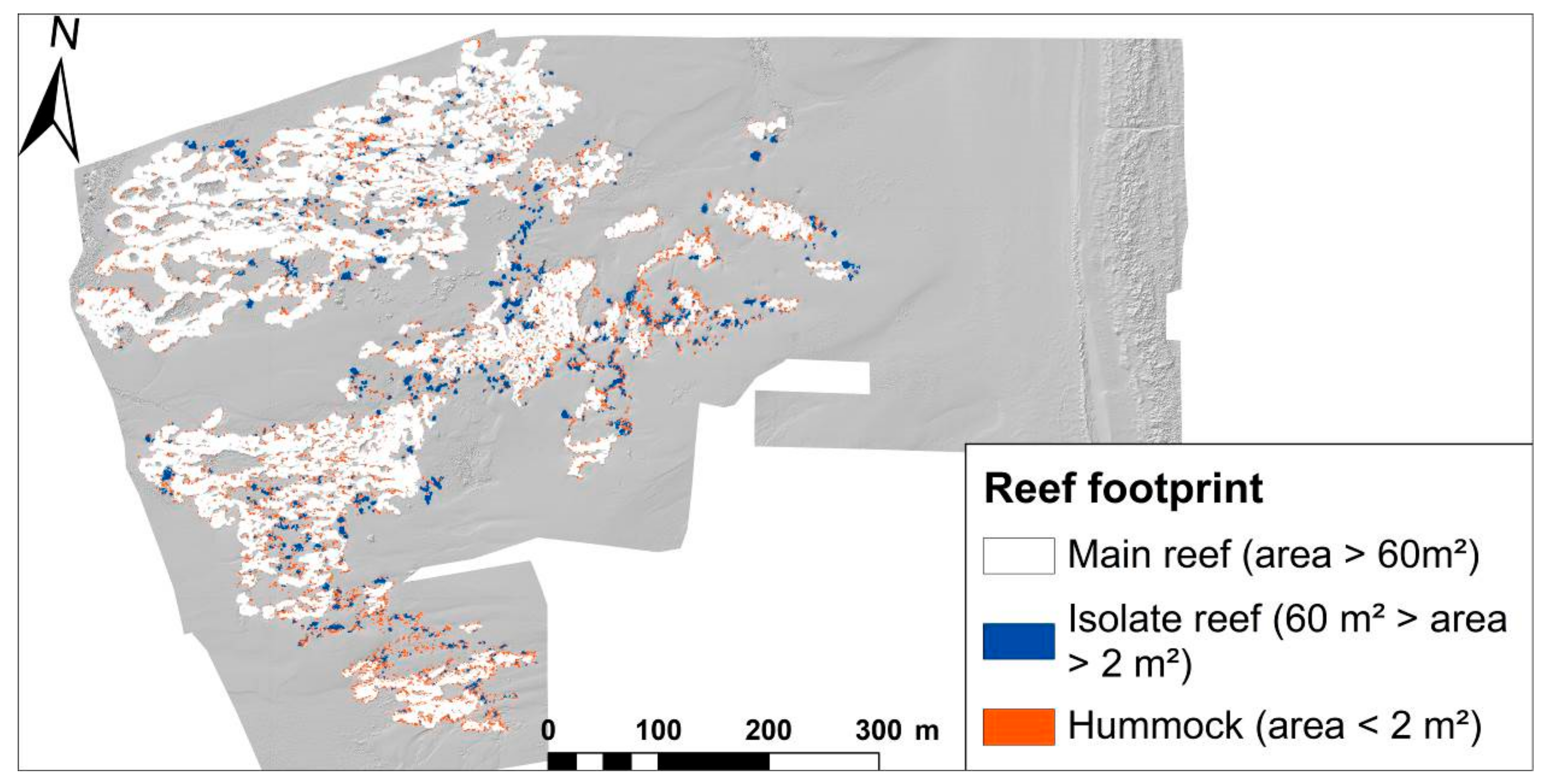
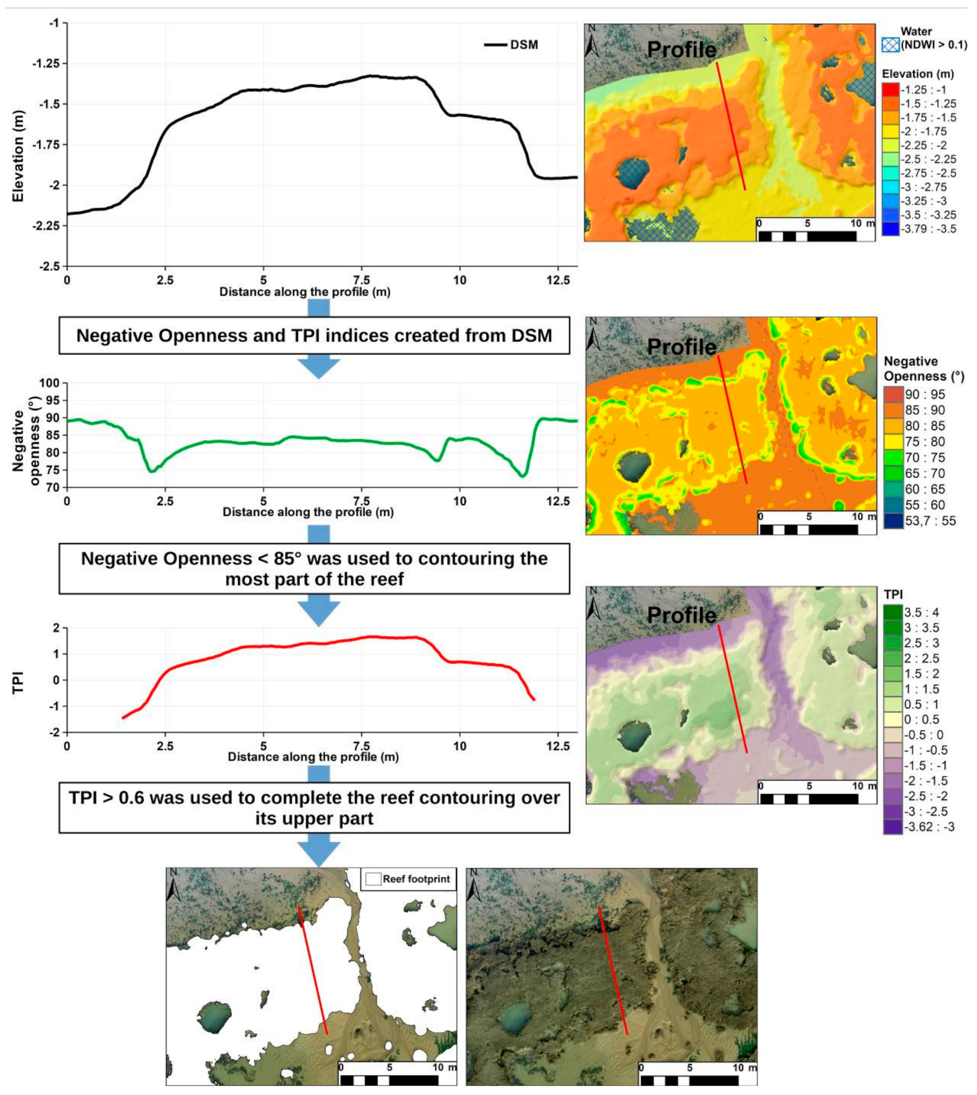
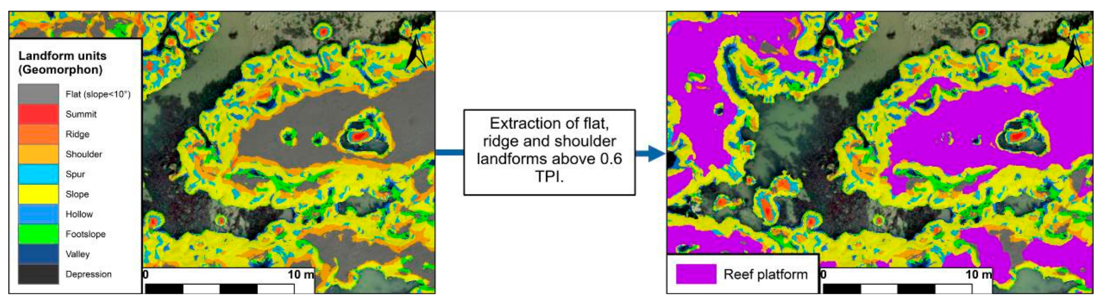
2.4. Reef Contouring Using Topography from DSM

The accurate elevation model represented a robust dataset for mapping the reef through landform analysis. Among many topographic attributes we selected indices that (1) are independent of cross-shore elevation changes, (2) highlight steep landforms such as reef flanks, (3) normalize elevation relative to the adjacent background sediment to identify the reef top, (4) are easy to compute and understandable for non-specialists in landform analysis. Two indices matched these conditions: the Topographic Openness (TO) [42], and the Topographic Position Index (TPI) [41]. The TO has been related to how wide a landscape can be viewed from any position [42]. It expresses the openness (positive openness) or enclosure (negative openness) of a landscape location in degrees or radian units. The topographic positive openness (TPO) (also called dominance) of landforms was represented as the mean angle openness from the zenith point of view, while the topographic negative openness (TNO) or enclosure was represented as the mean angle masked by surrounding topography from the nadir point of view [42]. The TPI compared the elevation of each pixel in a DSM to the mean elevation of a specified neighborhood around that pixel [41]. The TNO was very useful to map steep surfaces such as the reef flanks, while the TPI was used to map the top of the reef which is less enclosed than the reef flank topography. The TNO parameter was calculated in degrees from 8 directions and with a window of 2 × 2 m to match with the metric-scale width of the reef. The TNO was the most reliable index to identify reef flanks with a fixed threshold of negative openness ≤85° (Figure A2). The TPI was calculated with a 10 × 10 m kernel window to integrate sufficient surface areas from the adjacent background sediment and to highlight upper elevation pixels such as the top of the reef. A threshold of TPI ≥ 0.6 was set to identify the upper part of the reef (Figure A2). This threshold corresponded to the upper part of the reef flanks. The thresholds over TNO and TPI were combined to map the reefs (Figure A2). These two indices were obtained through System for Automated Geoscientific Analyses (SAGA) which is a Geographic Information System (GIS) toolbox [57].
Figure A2 describes the workflow integrating the combination of the two indices to map from the foot slope to the top of the honeycomb worm reefs. The first step consisted in removing from the DSM areas subjected to noisy and bad topographic modelling such as the water bodies typically found in intertidal areas [53,58]. Water bodies (intertidal pools and channels) were mapped and removed from the DSM using a simple threshold based on the Normalized Difference Water Index (NDWI) following Equation (1) [59]:
N D W I = G N I R / G + N I R ,
where G is the green band (560 nm +/− 16 nm) and NIR is the Near-Infrared band (840 nm +/− 26 nm) from the multispectral orthophotograph. The threshold retained to map water bodies was NDWI ≥ 0.1 (Figure A2). The reefs were classified with regards to the area of their footprint (Figure A2). Three classes were distinguished using the Jenks natural breaks method applied to the distribution of reef footprint areas: the main reef composed of connected and continuous biogenic structures, large reef structures with a projecting surface <60 m2, and isolated reef clumps <2 m2.

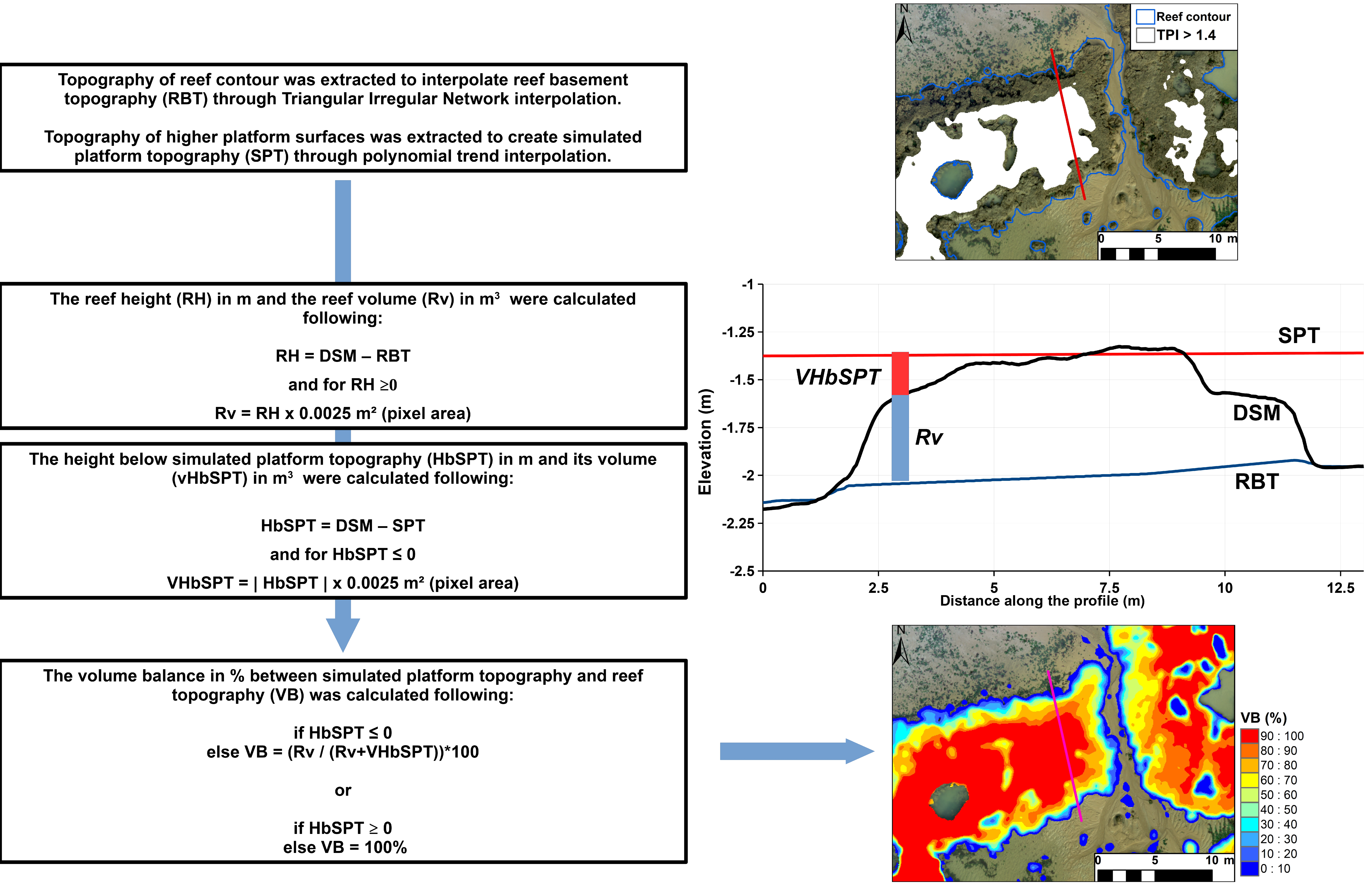
2.5. Reef Morphology Assessment

Honeycomb worm reefs developing on sandy substrates display a large variety of complex three-dimensional structures in different evolutionary phases [1]. Each type can be observed in a progradation (growth) or retrogradation (degradation) phase. Retrograding reef parts exhibit numerous marks of fragmentation such as block collapse, surface alterations, and irregularities in shapes. Describing the complexity of these landscape characteristics is challenging and landform analysis was tested to see which information could be retrieved.
The reef landforms were mapped by applying the “Geomorphological phenotype” method [43], named “Geomorphon”, to classify landforms from the DSM elevation (Figure A3). The Geomorphon method allowed classifying 10 types of landforms: flat surfaces, peaks, ridges, shoulders, spurs, slopes, pits, valleys, footslopes, and hollows [43]. The Geomorphon method was used to first describe reef landforms and then to map tabular reef shapes. This method is based on image texture similarity concepts [60] using the elevation of a point of interest relative to its neighbors, and secondly on a line of sight concept [42] which examines the degree of terrain openness along eight principal compass directions. Thus, Geomorphon provided a high degree of terrain autocorrelation [61], detecting transition between landforms. This method was used with its current implementation into SAGA GIS software [57]. This tool was set with a 2 × 2 m window and pixels were considered as flat landforms with a <10° slope (Figure A3). We set this window size to match the metric-scale width of the reef and to highlight landform diversity by limiting the terrain autocorrelation. Tabular shaped platforms on the top of the reef were characterized by flat, summit, and ridge and shoulder landforms. As flat landforms from the adjacent background sediment can also be selected, a threshold was set at TPI > 0.6 to select flat landforms of the upper parts of the reef. Shoulders, summits, and ridge landforms were aggregated to flat landforms if they were spatially joint (Figure A3), thus enabling the mapping of complete tabular platform features.
The last part of the morphological analysis was (1) to estimate the height of the reef (RH) with its foot toe elevation as a vertical reference, and (2) to calculate the volume of the reef (RV) and compare it to a theoretical and modelled fully tabular reef volume (Figure A4). The height of the reef was calculated by interpolating the reef basement topography (RBT) over the entire reef area. The reef basement elevation was extracted from the DSM by applying a 10 cm buffer to the reef contour (Figure A4). The interpolation of the reef basement level was simulated through a Triangulated Irregular Network (TIN) from the ESRI ArcGIS software. RH was obtained by subtracting reef basement level from reef DSM elevation (Figure A4). RV was calculated by multiplying RH by the pixel area for positive reef height (RH ≥ 0) (Figure A4). A theoretical tabular reef volume was built by modelling the reef top level from the topography of upper and tabular reef areas. These areas were selected by using a threshold of TPI > 1.4. The simulated platform topography (SPT) was modelled using a global polynomial function of rank 3 from the “Trend” toolbox in the ArcGIS software. SPT represented the elevation of the reef assuming that it has a full tabular shape. SPT was subtracted from the reef DSM, providing the height below SPT (HbSPT). This height was then used to calculate a reef volume below SPT (VbSPT), for the pixels where HbSPT < 0. Indeed, the DSM crossed the SPT level for some surfaces due to the high irregularity of the reef topography. Regarding these cases, the theoretical tabular reef volume was considered as equal to RV. The reef volume balance (VB, %) was calculated by comparing RV to a theoretical tabular reef volume (RV + VbSPT). VB is used as a proxy describing the tabular state of the reef ranging from 0 to 100 % when the reef is totally made up of a platform. The platform landforms coverage and the reef volume balance (VB) were summarized into a regular grid of 1 × 1 m covering the study area.

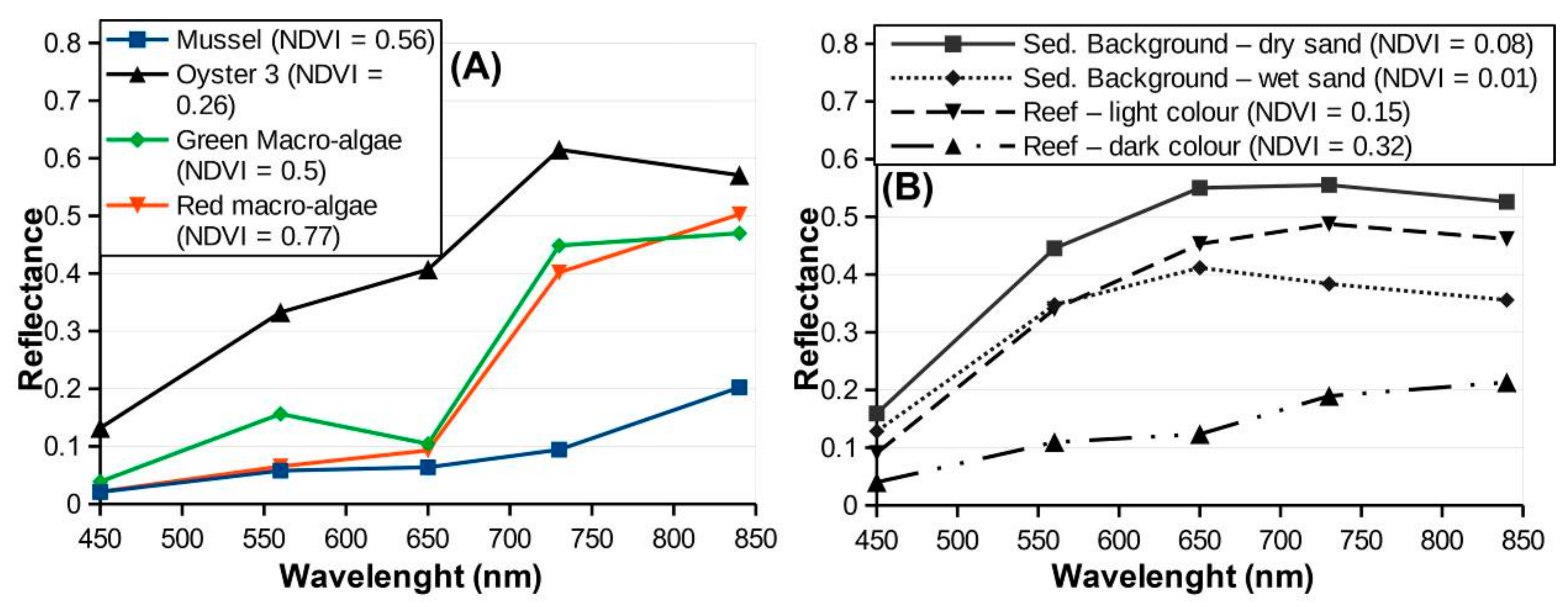
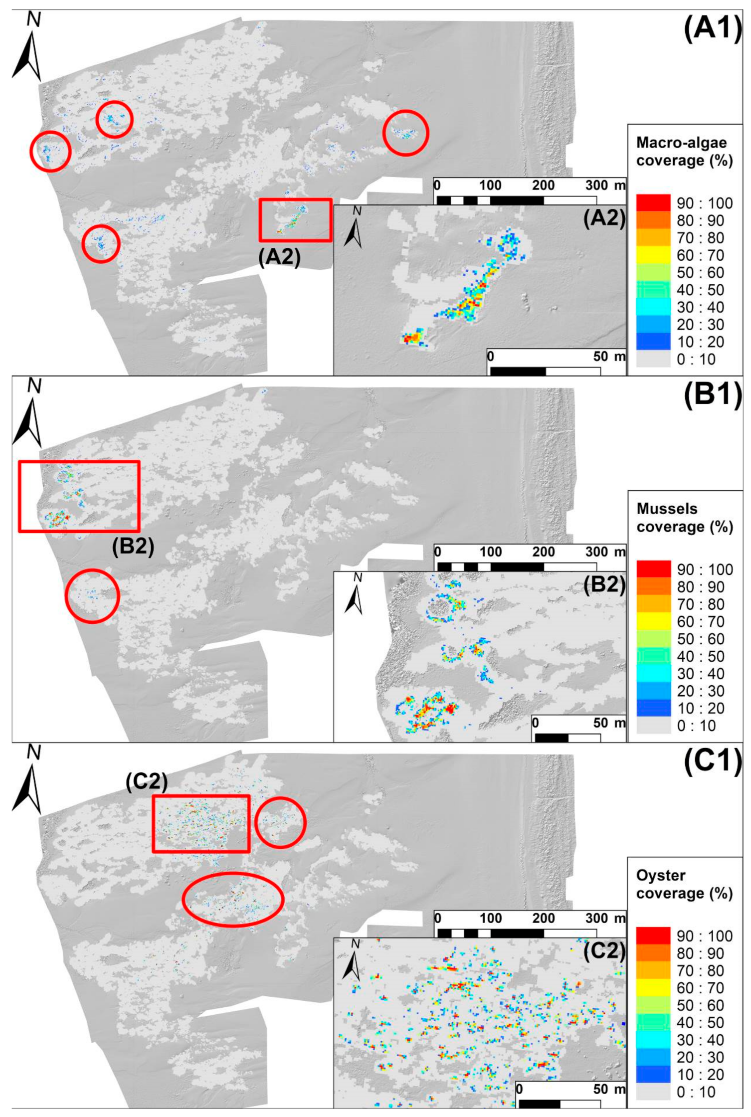
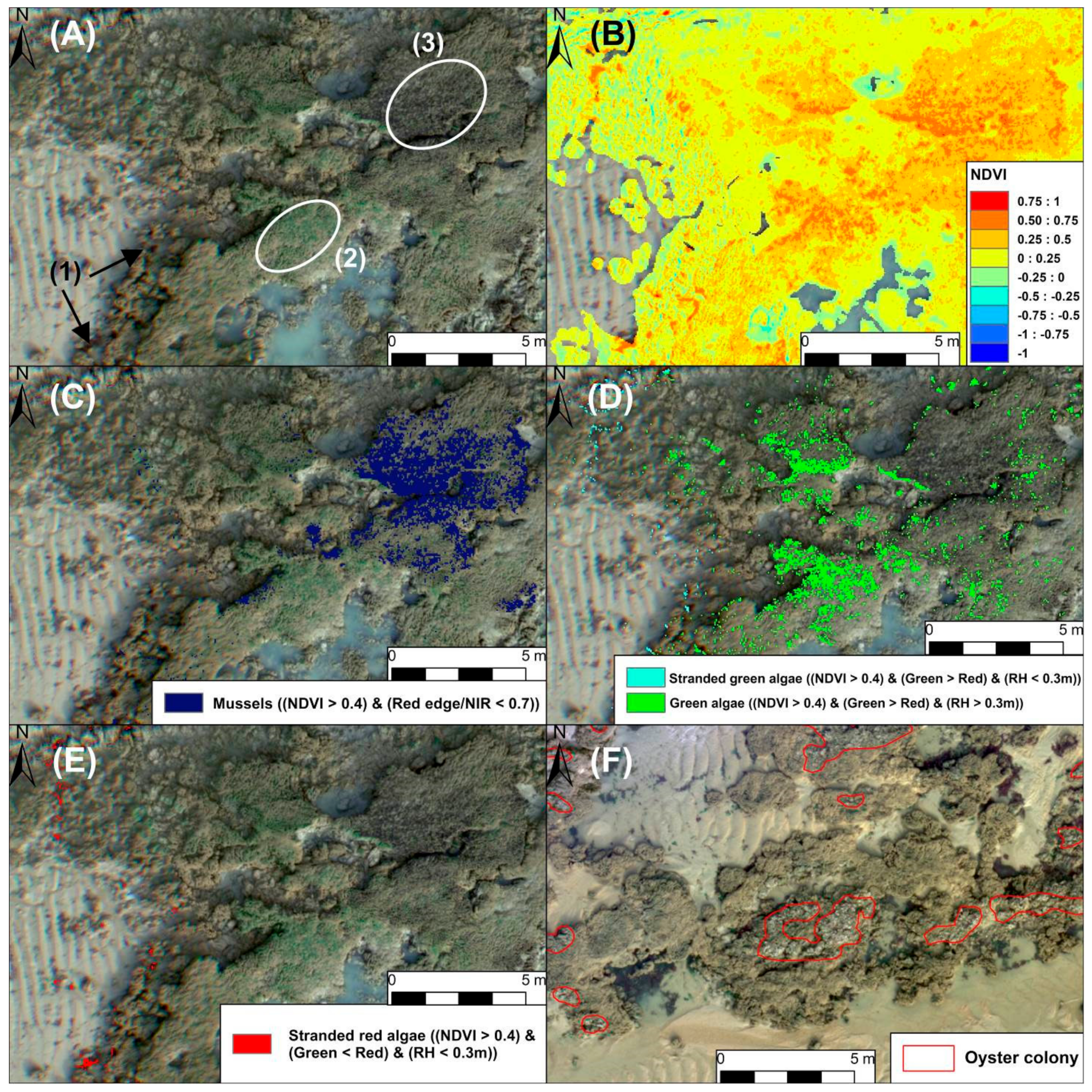
2.6. Reef Epibionts Mapping

Epibionts such as macroalgae and shellfish adversely affect honeycomb worm populations and their associated fauna [16]. Multispectral images were used to map two types of macroalgae, those attached to the reef (the green macroalgae Ulva spp.) vs. those brought in by tides from subtidal areas (mainly red macroalgae dominated by Soliera chordalis, sometimes mixed with a small proportion of green macroalgae) and stranded, as well as two bivalves, oysters Crassostrea gigas and mussels Mytilus edulis (Figure A5). Spectral indices based on their spectral properties combined with reef height were used for their discrimination. Macroalgae and mussels had Normalized Difference Vegetation Index (NDVI) [62] values higher than 0.4. The NDVI index was calculated following Equation (2):
N D V I = N I R R / N I R + R ,
G m i n R = G R .
Differences between Red and Green algae were highlighted by a simple Green and Red bands comparison named GminR index (Equation (3)). Red algae absorbed in the green band (GminR < 0) while green algae are more reflective (GminR > 0) [63]. The green macroalgae attached to the reef were identified with a double condition of a reef height above 0.3 m, to avoid the stranded algae at the basement of reef, and a GminR index > 0.
Wild oysters were spread over the reef, forming small and heterogeneous patches. They were sometimes covered by sand and surrounded by a darker unidentified biofilm. As a consequence, the oyster spectrum was very variable with no specific spectral shape and we were not able to find a spectral index or any method combining landforms for their discrimination. Their mapping was consequently made manually by photo-interpreting the RGB image.
The quality assessment of epibiont mapping was done through a confusion matrix using in situ field observations (n = 28) based on 0.25 m2 quadrats, and with additional locations mapped from the very high resolution orthophotograph. The assessment metrics were the User and Producer accuracy and the overall accuracy [64].

3. Results

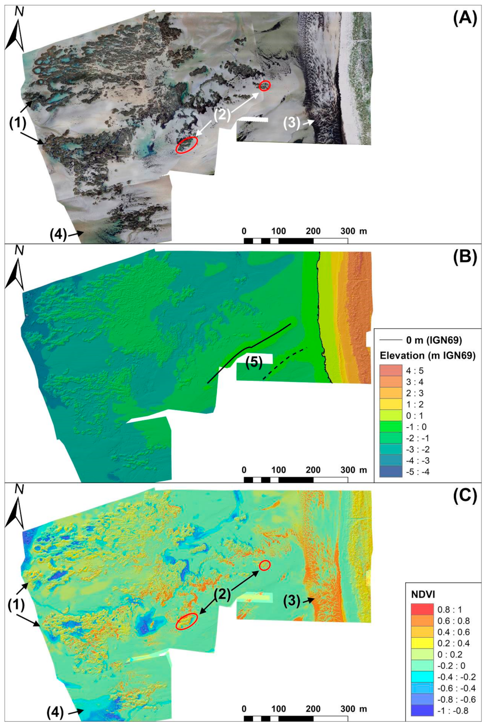
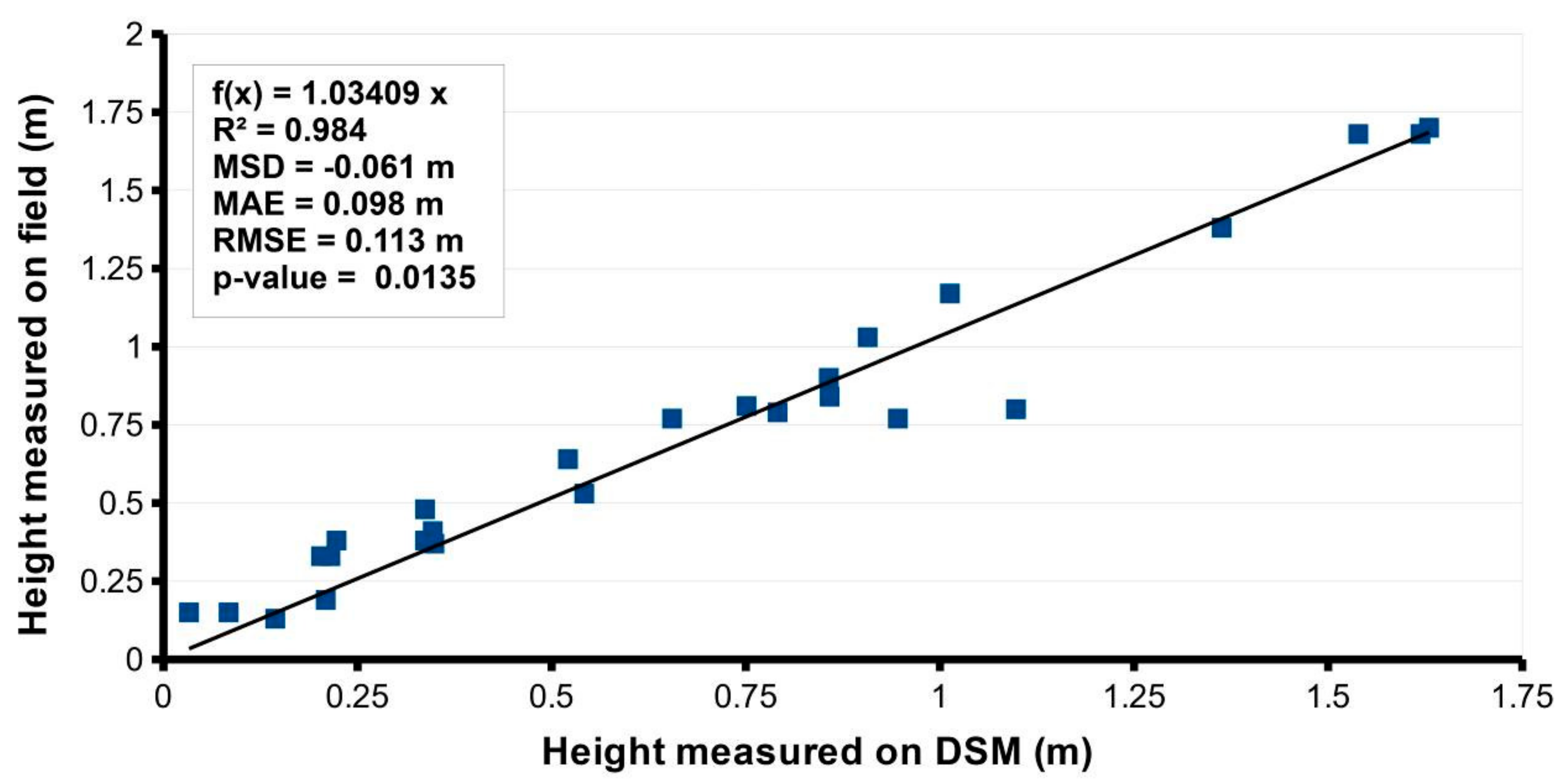
3.1. Multispectral and DSM Accuracy Assessments

The SfM photogrammetry end-products included a 5-band orthorectified multispectral image and a DSM with respective resolutions of 2.6 cm/pixel and 5.26 cm/pixel (Table 1 and Figure 2A,B). The DSM was resampled at a resolution of 5 cm/pixel to match the grid geometry that summarized the reef analysis results. The cloud point used to build the DSM had a density of 361 points/m2 (Table 1). The vertical accuracy was evaluated using field measurements which provided a MSD of -6.1cm with an MAE of 9.8 cm and an RMSE of 11.6 cm (Table 1 and Figure 3). The behavior of the vertical reconstruction error showed a distribution centered between −20 and 10 cm of elevation difference between the DSM and field measurements, with more than 70% of the observations between −20 and 0 cm (Figure 3). Consequently, the DSM production underestimated the elevation compared to field measurements.
The multispectral images also showed some brighter or darker areas located mainly over a number of highly reflective surfaces such as dry or wet sand (Figure 2A). However, these effects did not affect multispectral indices such as the NDVI, and bright/dark areas were not visible on the index map (Figure 2C). The spatial distribution of the NDVI over the reef showed the presence of large areas covered by stranded macroalgae next to the beach (Figure 2C, zone 3 with NDVI > 0.6) while some were observed between reef patches.

3.2. Reef Contouring

The reef was composed of large connected structures and large water pools were observed within the reef in the lowest intertidal areas (Figure 2A). The swash platform presented swash bars, pools, and flat surfaces with a regular onshore gradient (Figure 2B). Topographic changes and reef morphology presented strong contrasts compared to the flat and smooth surfaces of the swash platform. The reef flanks exhibited steep slopes while the reef height ranged between 0.2 and 1.5 m. The DSM topography itself was not directly usable because it was subjected to an elevation gradient ranging between −3 m and 0 m from the lowest intertidal areas to the beach toe (Figure 2B). The DSM elevation was used to calculate two morphometric indices (TPI and TNO) and to apply a landform classification. TPI ranged from −3.41 to 4 and the TPI threshold set at 0.6 selected areas from the mid-slope of the reef flanks to the top of the reef (Figure A2). TNO ranged from 43° to 100° and the TNO threshold set at 85° selected areas between the reef foot slope and the upper part of reef flanks (Figure A2). The combination of TPI and TNO thresholds identified reef structures from the smallest isolated hummocks to the largest structures, excluding inner low-lying flat surfaces of the swash platforms, bottoms of depressions from inner reef collapse, or the bottoms of narrow valleys between different reef structures (Figure 4). The reef structures covered an area of 0.81 km2 (or 8.15 ha) over the swash platform (Figure 4). Continuous biogenic structures covered 89.35% (7.28 ha) of the whole reef surface, while large isolated reef structures (with a projecting surface comprised between 2 and 60 m2) covered 7.61% (0.62 ha). Isolated small reef clumps covered 3.04% (0.25 ha) (Figure 4).
Figure 2. SfM photogrammetry end-products. (A) Orthophotographs at a resolution of 2.6 cm/pixel. (B) DSM at a resolution of 5 cm/pixel referenced to IGN 1969 vertical datum. (C) NDVI index at a resolution of 2.6 cm/pixel. Several elements were identified from the orthophograph, DSM, and NDVI index: (1) reef structures composed of dark sand, difficult to distinguish from background sediment using spectral indexes such as NDVI; (2) green macroalgae colonizing the reef with intermediate NDVI values (0.4 to 0.6); (3) macroalgae washed up on the beach composed mostly of red macroalgae, with high NDVI values (above 0.6); (4) water bodies with low NDVI values (below −0.1); (5) cross-shore swash bars, typical of ebb delta morphologies, observed on the DSM.
Remotesensing 14 00307 g002
Table 1. SfM photogrammetry end-product quality assessment metrics.
SfM Photogrammetry End-Product
Number of images per band4716
Dense point cloud density361 points/m2
Raw multispectral resolution (cm/pixel)2.6 cm/pixel
Raw DSM resolution (cm/pixel)5.26 cm/pixel
Field validation
Field Validation number used29
Vertical accuracy MSD−6.1 cm
Vertical accuracy MAE9.8 cm
Vertical accuracy RMSE11.3 cm
Figure 3. Error of vertical reconstruction of the DSM. Plot of reef height measured on the DSM against reef height measured in the field.
Remotesensing 14 00307 g003
Figure 4. Mapping of the reef footprint in three main classes: the main reefs (area > 60 m2), isolated reefs (60 m2 > area > 2 m2), and hummocks (area < 2 m2).
Remotesensing 14 00307 g004

3.3. Reef Morphology

The spatial distribution of reef heights showed that the highest reef was located in the lowest part of the swash platform, with reef heights > 1 m. The lowest reef heights were located in the inner reef area with values comprised between 0 (i.e., the same height as the sediment surface) and 0.4 m (Figure 5A). The presence of a reef platform and the degree of morphological fragmentation of reef platforms were estimated respectively by the percentage of platform surface and the reef volume balance index (Figure 5B,C). The platform shape mapped by selecting flat landforms on the upper part of the reef from “Geomorphon” landform classification was expressed in percent cover (Figure 5B). Large tabular platforms with a coverage >70% were located mostly on the western and eastern borders of major reef structures (Figure 5B). The inner part of reef structures and the eastern part of the study area had the lowest coverage in tabular shape platforms. These spatial distributions were confirmed by the volume balance index (Figure 5C). Tabular shape platforms presented a volume balance exceeding 70%, while fragmented and/or other reef shapes were observed below this value.

3.4. Epibiont Mapping

Epibiont coverage by mussels and macroalgae was mapped using multispectral indices, while oysters were identified by photo-interpretation (Figure A5). Figure 6 shows examples of reflectance spectra from the main epibionts: green algae colonizing the reef (Ulva sp.), drifting red algae deposited at the base of the reef (dominated by Solieria chordalis), mussels and oysters. Green and red macroalgae shared similar reflectance in the NIR, but the latter absorbed more light at 560 nm. Mussels were the least reflective object notably in the NIR (Figure 6A). Reefs with a light brown color showed a similar reflectance spectrum compared to the background sediment, while dark brown to grey reefs had a spectral signature with a lower albedo and were highly heterogeneous (Figure 6B). The confusion matrix showed an overall accuracy of 88.8% indicating that the results of the classification were accurate (Table 2). The producer accuracy for mussels, green macroalgae on reefs, stranded green and red macroalgae, were respectively of 99.68%, 79.62%, 87.21%, and 100%. The green algae colonizing the reef were more difficult to detect because they were less developed and had NDVI values below the threshold of 0.4. The stranded red macroalgae and the mussels colonizing the reef were mapped with a high accuracy.
Figure 5. Reef morphological assessment. (A) Reef height in m. (B) Coverage in percent of platform landforms summarized into 1 × 1 m grid. (C) Volume balance representing the real reef shape volume compared to a theoretical tabular reef, summarized into 1 × 1 m grid.
Remotesensing 14 00307 g005
Green macroalgae colonizing the reef were mostly distributed on the western and eastern borders of the reef area with a coverage seldom higher than 40%, representing 732.6 m2 and 0.9% of the reef footprint area (Figure 7(A1,A2)). Their presence was associated with less or mildly fragmented reefs with a VB ranging from 40% to 80% and lower isolated reefs with a reef height ranging from 0 to 0.50 m (Figure 4 and Figure 5A,C). Mussels were exclusively located on the western part of the reef with a few grid cells showing a 100% cover, representing 67.6 m2 and 0.08% of the reef footprint area (Figure 7(B1,B2)). Their location corresponded to the low intertidal part of the swash platform and they were mostly established on higher platform surfaces with a VB ranging from 70% to 100% (Figure 2B, Figure 5C and Figure 7(B1,B2)). Oysters were mostly observed on the inner part of the northern reef (Figure 7(C1,C2)) and their locations corresponded to fragmented inner reef parts with a VB mostly below 70% (Figure 5C). Oysters covered 1251.2 m2, representing 1.53% of the reef footprint area.

4. Discussion

The UAV survey coupled with SfM photogrammetry has provided the first very high-resolution image of the honeycomb reef of the Fromentine delta on the French Atlantic coast. The DSM was used to assess ground elevation and apply topographic indices combined with multispectral data. With a spatial resolution of 2.63 cm for multispectral data and 5 cm for the DSM (Figure 2A,B), the reef extent was identified from the smallest isolated reef clumps to the largest tabular structures. The new index VB, estimating the percent cover of the platform-like structure, is proposed here. In spite of the low spectral resolution of the multispectral camera, macroalgae and mussels were satisfactorily identified, but this was not possible for oysters colonizing the reef.

4.1. Accuracy and Constraints of UAV Remote Sensing of Reefs

UAV and SfM photogrammetry technologies open new perspectives for mapping intertidal honeycomb reefs [35,36,37]. The ground-breaking work of Ventura et al. (2018) [35] provided a simple mapping solution through an OBIA approach. However, the topographic information was not fully exploited, considering variables such as fragmentation or reef morphotypes used in the establishment of a health status index [13]. This study explored topographic-based indicators that make good use of the very high-resolution multispectral images and the DSM. With a direct RTK GPS image geolocation, the DSM was built without the need for ground control points (GCP), in exchange for a slight decrease in vertical accuracy, which allowed mapping a wide area in a short time and without time-consuming preparations [65,66,67,68,69]. The 3D cloud point density was close to that generated by terrestrial LiDAR survey, thus enabling a very detailed definition of the 3D structures of the reef [70]. The 5-cm DSM pixel resolution revealed the high heterogeneity of reef topography. This very high DSM resolution allowed for the identification of isolated small reef clumps and fragmented parts of the reef which could be missed with air-borne LiDAR resolution [70]. The MSD, MAE, and RMSE between modelled reef height and field measurements were −6.1 cm, 9.8 cm, and 11.3 cm, respectively, in the range of other studies that used only RTK GPS position of photographs to build 3D models [65,66,67,68,69]. The accuracy could have been enhanced with GCPs [67], but it was sufficient for the purpose of mapping the reef footprint and for building various indices related to reef geometry. A poor reconstruction of the topography occurred over areas with water such as depressions, channels or flooded low intertidal areas. This issue is well known with SfM photogrammetry [53,54,58], and requires the use of topographic or spectrometric filters. In this study, the multispectral camera was used to map and remove water-filled areas by applying the multispectral water index NDWI. The orthophotograph presented some brighter and darker areas, with the darkened zones corresponding to a momentary decrease in incoming light, which led to lower reflectance values. Brighter areas appeared also over reflective surfaces such as dry sand or wet sand due to sun glint, in spite of the flight plan perpendicular to the sun. However, these darker or brighter areas were not visible anymore on NDVI and NDWI images, indicating that spectral indices were less sensitive to irradiance changes [71]. Eventually, there are constraints related to UAV flight regulations that condition their operational range of flight, the surveyed area and image resolution. The DJI Phantom 4 Multispectral, with a lightweight of 1.49 kg, belongs to UAV European class C2, and is authorized to fly in every scenario stipulated in French national and European Union regulation frameworks. However, like numerous stretches of the coast of France, the Fromentine delta is subject to military regulations that require the UAV pilot to maintain a visual line of sight with a maximum distance of 200 m. This limitation increases the number of flight paths to cover the reef and requires moving the RTK base station both of which lengthen the duration of operations that is, conversely, constrained by the tide.

4.2. Identification of the Reef Footprint

Mapping the reef footprint was not possible from a solely multispectral approach. The main issue was the spectral similarity between the reef itself and the sand deposits of the swash platform. This constraint was earlier observed by Marchand and Cazoulat (2003) [25] with the HRV-XS multispectral sensor of the SPOT-3 satellite. The Phantom 4 Multispectral UAV has only five bands. This problem can now be overcome with a higher hyperspectral resolution, as demonstrated by Bajjouk et al. (2020) [27], but this is not very accessible and is a costly technology. In the healthy parts of the reef, the tubes are built up with resuspended sand grains and have a similar color to the surrounding sediment [1]. However, the reef displayed a complex 3D structure on the DSM, contrasting with the flat or mild slopes of the background sediment. These shape differences between the complex reef structure and the flat or smooth topography of background sediment were used in this study to map the reef footprint with topographic indices. Nevertheless, background sediment elevation along the swash platform is susceptible to short-term changes due to sediment movement during tidal cycles associated with alongshore migration of swash bars and local sediment deposition or depletion related to reef hydrodynamics, both of which generate variations in topography [48,72,73,74]. The raw topography was, therefore, not considered reliable for mapping the reef, in contrast to information regarding slope changes, relative topographic positions [41] or topographic openness/enclosure [42]. The TNO was less sensitive to raw elevation changes and could be operated over any 3D model to highlight structures exhibiting complex shapes [42]. In the present study, the TNO index was used to map the flanks of the different reef structures from the foot slope to the top of the reef. The radius to calculate the line of sight from the nadir point of views was 2 m in order to detect small ball-shaped structures. The main issues encountered were that small structures on the background sediment such as ripples marks were also detected and needed to be removed (filtered by area), and that some parts of the reef platform were less enclosed and were out of the threshold range. The later issue was overcome by considering another index: the TPI calculated with a radius of 10 m in order to take into account the topography of the background sediment. The TPI is a scale-dependent metric, which imposes choosing the right scale to detect the right landscape. The TPI calculation scale was especially large to comprise the ebb delta platform elevation surrounding the reef. The TPI did not detect well the reef basement and hummocks, partly confounded with the background, but was very efficient in mapping the top of the reef, and was therefore complementary to the TNO index. The reef footprint was mapped considering a gradient encompassing the largest reef structures, but also smaller clusters of coalescent structures, and finally the smallest isolated clumps (Figure 4). The latter could not be identified with a 50-cm image resolution from optical airborne data [27]. Hummocks and small coalescent structures were abundant in transition zones between the main reefs in the southern and eastern parts of the study area (Figure 4). Mapping small ball-shaped structures provides relevant information on the dynamics and the prograding phase of the reef [1,75]. The reef had a total surface of 8.15 ha compared to the 223 ha for the largest European reef, the Sainte-Anne reef of Mont-Saint-Michel bay [22]. The average reef height was 23.11 cm with a standard deviation of 26.18 cm, a value not far from the 35.3 ± 9.1 cm of the Sainte-Anne reef (2007 data) [13], but the Fromentine reef had a very high heterogeneity compared to the latter reef. The highest structures in our study area reached 190 cm in the western low intertidal area, compared to 75 cm for the Sainte-Anne reef. In the Sainte-Anne study, the reef height was calculated by levelling the DSM with a reef basement elevation model. Reef height is a variable that strongly depends on changes in the background sediment elevation. The reef can be locally very high compared to other areas due to local depletion of the background sediment, or, conversely, very low due to sediment accretion. This information is important because one of the causes of the regression of the reef in the past was silting up by sandbanks [8,9]. The sediment dynamics and mobility of the sandbanks are related to the functioning of the tidal delta, and to the position of the main tidal channel, which is characterized by marked oscillations [46].

4.3. Topographic Analysis

The Geomorphon classification combined with the Topographic Position Index (TPI) was used to identify flat landforms of the upper parts of the reef, i.e., the platform stage [75]. Continuous flat areas with a platform-like morphology correspond to what was previously described as a reef with good health status [13]. Upper flat, summit, ridge, and shoulder landforms were selected from the Geomorphon types to identify flat landforms [43]. These landforms characterized the upper part of the reef structure and were spatially connected as upper flat landforms, or summits, or ridges representing the relief apex, then as shoulder landforms representing the upper part of the slope. The extraction of these platform features was carried out with a TPI threshold to ensure that only the top of the reef was concerned and to avoid the inclusion of flat landforms from the adjacent background sediment. The threshold was selected to correspond to the mid-slope of landforms. TPI was the main topographic index used here because of its performance and understandability for non-specialists, but there are others topographic indices and landform classifications that could have been used to detect reef top such as Fuzzy Landform Element Classification [76,77] or Multiresolution Index of the Ridge Top Flatness (MRRTF) [77,78]. The spatial distribution of reef platforms showed a peripheral pattern as these platforms were mostly located over the external part of the northern and south-western reefs (Figure 5B). The internal areas had a platform coverage <70%, which corresponded to a higher reef fragmentation. The eastern part of the reef close to the beach presented the most fragmented structures with important spatial discontinuities that explain the low platform coverage below 40%. In fact, this is the most accessible part of the reef and probably the most vulnerable to human trampling by recreational fisherman [21]. The platform feature coverage index was useful by providing an overview of platform spatial distribution but did not allow for quantification of the morphological state of the top of the reef. The index developed in this study to estimate quantitatively the fraction of platform-like morphology was the reef volume balance index (VB) (Figure 5C). The VB index was useful to distinguish the continuous platform from fragmented reef areas. The latter were clearly identified by VB values below 50%. This index was also not sensitive to local topographic changes of the background sediment, which can lower or increase the reef height and reef volume. The reef real volume was simply compared to the theoretical platform-shaped reef volume. The VB index, contrary to the platform coverage index, yielded a more continuous display of reef platform structure locations. It confirmed the observations made with the platform coverage index but highlighted also that platform features occurred over isolated reef clusters in the eastern areas. The main issue with this index was its building process, which requires interpolating both the reef basement topography (RBT) and the simulated platform topography (SPT). RBT interpolation was based on the TIN method. The TIN method is probably one of the simplest spatial interpolation techniques and is very accurate when there are dense and clustered topographic observations. The topographic observations used with the TIN interpolation method came from the external border of the reef footprint, which had close patterns with a high density of records related to DSM resolution. The TIN method also does not smooth the interpolation, and this is useful in building a straight plan for the RBT. The SPT was obtained with a polynomial trend interpolation to provide a plan which almost crossed the local topography of the platform.

4.4. Epibiont Mapping

The reef dynamics are influenced by the presence of macroalgae and bivalve molluscs colonizing the reef surface and which exert a spatial competition with the polychaetes. These epibionts tend to colonize degraded reefs corresponding to a retrogadation phase [1,13,16]. In this study, mapping of epibiont coverage was achieved through the combination of radiometric and topographic indices (Figure 5). The global accuracy of the confusion matrix of 88% (Table 2) was in the range, or higher than, comparable studies [36,79,80]. The green algae Ulva sp. growing on the reef itself can alter the population dynamics of S. alveolata by preventing the settlement of new recruits [16]. In this study, the challenge was, firstly, to differentiate green algae from red algae, and, secondly, to identify the macroalgae colonizing the reef from the accumulation of stranded macroalgae found at the base of the reef and filling up depressions inside the reef. In fact, red macroalgae do not grow on the reef, but are exported from subtidal rocky zones, dislodged by storms and the strong hydrodynamic conditions prevailing in the area. They form much of the litter covering the swash platform and accumulating at the reef basement. Some green algae were, however, observed mixed with the stranded red algae. The spectral resolution and camera sensibility were sufficient to distinguish green and red algae based on green and red band ratios (Figure 6 and Figure A5). Nevertheless, the spectral indices used solely, could not distinguish green algae growing on the reef from the stranded ones. A topographic index was, therefore, necessary in combination with a spectral index to identify green algae growing on the reef. The reef height (RH) was, therefore, applied to detect green algae growing from the mid slope of reef flanks to the top of the reef (Figure A5). This epibiont covered only 0.9 % of the total reef surface and was mainly found in reef areas with fragmented morphologies, as observed by Gruet (1986) [75]. The mussel detection based on a red-edge normalized to NIR band index showed a high accuracy (Table 2). The black mussel shells displayed a characteristic low reflectance in the visible and the red-edge (Figure 6). Mussels were mainly found in the lower intertidal part of the reef growing on platforms and competing for space with S. alveolata (Figure 7(B1,B2)). There are mussel farms less than one kilometer to the north of the reef, but, surprisingly, only very small reef surfaces were covered by mussels (0.08%). Depending on location, various epibiont species can colonize the reefs. For example, the oyster C. gigas extensively colonizes the reef of Mont-Saint-Michel bay [13,16]. Oysters could not be mapped based on their spectral signatures and their distribution was photo-interpreted (Figure A5). Photo-interpretation was time-consuming, but feasible thanks to the very high image resolution. Bajjouk et al. (2020) [27] similarly observed the large spectral variability of oysters colonizing S. alveolata reefs. Oysters could reach a high density in the degraded parts of the reef with variable orientations of the shells, from horizontal to vertical [26], sometimes covered by sand (Figure 5C and Figure 7(C1,C2)). They can show absorption at 675 nm (Figure 6) [27], as their shell is colonized by unicellular photosynthetic organisms [81]. They were also observed on steep surfaces such as reef flanks but with a sparse spatial distribution. A higher spectral resolution may not solve this problem [26] but a perspective could be to test a segmentation approach, using an object-based image analysis [82,83]. Oysters were located in the most degraded part of the reef where they exert a strong spatial competition, growing over S. alveolata tubes (Figure 5C and Figure 7(C1,C2)) [16]. They attract recreational fishermen that use destructive methods to collect these oysters from the reef [6], and this exacerbates the significant negative impacts of trampling [21].

5. Conclusions

S. alveolata intertidal reefs showed a high heterogeneity of shapes and spectral responses. They can be confounded with a sandy background, especially with coarse resolution sensors such as EO satellites. The present study highlighted the possibility to map the reef footprint, shape, and spatial distribution of epibionts from a combination of spectral and topographic analysis of UAV-based multispectral orthophotograph and DSM. For the topographic dataset, we recommend at least RTK corrections for the UAV, with, if possible, a Ground Control Points (GCP) coverage. The topographic analysis can be done with a standard RGB sensor but the multispectral data was useful to map the epibionts. High-resolution multispectral datasets processed with the SfM photogrammetry technique provided centimeter-resolution orthorectified multispectral images and DSM. The DSM was used to (1) map the reef footprint through topographic indices such as the TNO and TPI, (2) to evaluate reef morphological state through platform shape-like mapping from the Geomorphon method and the VB index, and (3) identify macroalgae colonizing the reef. The multispectral orthophotograph and derived vegetation indices were used to map water bodies and epibionts colonizing the reef but the spatial distribution of oysters had to be photo-interpreted. This study has explored the possibility of combining and weighing all of these criteria to develop high-resolution metrics to assess the reef’s ecological status. Criteria based on reef color representing clear/dark/muddy sand need further consideration and will be investigated in future work. The present study exploited the potential of combining topographic analysis with spectral information in mapping intertidal habitats. This principle is transferable to other species building three-dimensional structures. There is potential wider applicability to bioconstructions made up by molluscs [34] and other polychaetes worms all over the world from the genus Idanthyrsus sp., Gunnarea sp., and Phragmatopoma sp. [84]. Finally, we have demonstrated that an affordable commercial sensor can provide high-quality quantitative data for policymakers for the management and conservation of this peculiar habitat.

Author Contributions

Conceptualization, G.B., S.O. and L.B.; methodology, G.B. and S.O.; software, G.B.; validation, Y.G., S.F.D. and L.B.; formal analysis, G.B.; investigation, G.B., S.O. and L.B.; resources, L.B.; data curation, G.B.; writing—original draft preparation, G.B. and L.B.; writing—review & editing, G.B., S.O., Y.G., S.F.D. and L.B.; visualization, G.B. and L.B.; supervision, G.B. and L.B.; project administration, L.B.; funding acquisition, L.B. All authors have read and agreed to the published version of the manuscript.

Funding

This research was supported by the EU BiCOME project (Biodiversity of the Coastal Ocean: Monitoring with Earth Observation) funded by the European Space Agency under “Earth Observation Science for Society” element of FutureEO-1 BIODIVERSITY+ PRECURSORS call, contract No. 4000135756/21/I-EF.

Institutional Review Board Statement

Not applicable.

Data Availability Statement

The data presented in this study are available on request from the corresponding author. The data are not publicly available due to data format and size.

Acknowledgments

We are thankful to the reviewers for their comments that helped to improve the manuscript.

Conflicts of Interest

The authors declare no conflict of interest. The funders had no role in the design of the study; in the collection, analyses, or interpretation of data; in the writing of the manuscript, or in the decision to publish the results.

Appendix A

Figure A1. Survey settings and SfM photogrammetry workflow. This workflow was composed of an image-acquisition and field survey phase (top panel), followed by image post-processing using the SfM photogrammetry workflow (middle and bottom panels). The acquisition of multispectral images was carried out using a UAV DJI Phantom 4 Multispectral following SfM photogrammetry dedicated flight plans, and the images were accurately geotagged through a DJI’ RTK GPS base station. Field validation of reef height and reef coverage type was set along 32 locations. The SfM photogrammetry workflow was carried out using Agisoft Metashape software. It corresponds to a classical workflow that has been described in numerous publications, excepting the correction from multispectral images to reflectance images through the UAV sunlight sensor. The outputs were a RGB and 5-band multispectral orthophotographs and a DSM at resolutions of, respectively, 2.7 cm and 5 cm per pixel.
Remotesensing 14 00307 g0a1
Figure A2. Honeycomb worm reef contouring from DSM processing and topographic indices. The protocol consisted in five steps. Firstly, water bodies were removed from the DSM elevation based on the NDWI index. The DSM elevation cleaned of water bodies was used to apply two topographic indices: the Topographic Openness (TO), of which only negative topographic openness (TNO) was used, and the Topographic Position Index (TPI). TNO values below 85° identified the major part of the reef, especially its flanks. TPI values above 0.6 completed the approach to map the upper part of the reef. The combination of these two indices enabled accurate mapping of the reef footprint from the ebb delta sediment surface.
Remotesensing 14 00307 g0a2
Figure A3. Mapping of reef platform landforms. This method was based on landform classification using the Geomorphological Phenotype, or “Geomorphon” [43], which classes and clusters elevation pixels into 10 classes of landforms (left panel). The flat, ridge, and shoulder landforms over the reef upper part were selected through TPI value of up to 0.6, which mainly corresponded to the middle of reef flanks.
Remotesensing 14 00307 g0a3
Figure A4. Estimation of reef volume balance compared to tabular reef state. This method consisted in comparing observed reef volume with a theoretical volume simulating a full reef platform. It was based on the use of the DSM elevation in combination with the reef footprint mapped previously. The first step of this method was to model the ebb delta platform elevation without the reef elevation to create a reef basement topography (RBT). This was carried out by extracting the DSM elevation along the external boundary of the reef footprint before interpolating it within the reef footprint through the Triangular Irregular Network (TIN) method. The raw DSM elevation was compared to the RBT to obtain both reef height (RH) in m and reef volume (Rv) in m3. RH had, in very restricted locations close to water-filled depressions, values below zero that were due to smooth interpolation of the RBT. These RH values were removed before creating the Rv. The Simulated Platform Topography (SPT) was built by using the higher part of the reef topography filtered with a high TPI threshold. The platform level was simulated by polynomial trend interpolation of the high reef topography. The SPT was compared to the DSM to measure the height in m below the SPT (HbSPT), then its volume in m3 (VHbSPT). The volume balance of the reef compared to the simulated platform shape (VB) was calculated by assuming that the theoretical platform volume was equal to the addition of the VHbSPT and Rv, which was compared to Rv. The volume balance expressed the percentage of theoretical platform volume represented by the measured reef volume. The SPT level was a trend that did not fit perfectly everywhere because of the heterogeneous reef topography. HbSPT values exceeding 0 were consequently filtered, and for these values, VB equals 100%.
Remotesensing 14 00307 g0a4
Figure A5. Mapping of epibionts such as macroalgae, mussels, and oysters over the reef structure. (A) Low intertidal reef with stranded red macroalgae (1) at the reef basement, green macroalgae growing over the reef (2), and mussel patches (3). (B) NDVI index highlighting macroalgae and mussel locations. (C) Mussel pixels were detected by extracting high NDVI pixels (NDVI > 0.4) and low red-edge/NIR bands (REbnNIR < 0.7). (D) Green macroalgae pixels were detected by extracting high NDVI pixels (NDVI > 0.4) and with a positive green-minus-red-band index (GminR > 0). The stranded green macroalgae at the reef basement were located in areas of low reef height (reef height < 0.3 m). (E) Red macroalgae pixels were extracted with high NDVI index values (NDVI > 0.4) and a negative green-minus-red band index (GminR < 0). (F) Wild oyster colonies were mapped by photo-interpretation of the orthophotograph.
Remotesensing 14 00307 g0a5

References

  1. Curd, A.; Pernet, F.; Corporeau, C.; Delisle, L.; Firth, L.B.; Nunes, F.L.D.; Dubois, S.F. Connecting organic to mineral: How the physiological state of an ecosystem-engineer is linked to its habitat structure. Ecol. Indic. 2019, 98, 49–60. [Google Scholar] [CrossRef] [Green Version]
  2. Curd, A.; Cordier, C.; Firth, L.B.; Bush, L.; Gruet, Y.; Le Mao, P.; Blaze, J.A.; Board, C.; Bordeyne, F.; Burrows, M.T.; et al. A broad-scale long-term dataset of Sabellaria alveolata distribution and abundance curated through the REEHAB (REEf HABitat) Project. Seanoe 2020, 2. [Google Scholar] [CrossRef]
  3. Nicoletti, L.; Lattanzi, L.; La Porta, B.; La Valle, P.; Gambi, M.; Tomassetti, P.; Tucci, P.; Chimenz Gusso, C. Sabellaria reefs from the Latium coast (central Tyrrhenian Sea). Biol. Mar. Mediterr. 2001, 8, 252–258. [Google Scholar]
  4. Ingrosso, G.; Abbiati, M.; Badalamenti, F.; Bavestrello, G.; Belmonte, G.; Cannas, R.; Benedetti-Cecchi, L.; Bertolino, M.; Bevilacqua, S.; Bianchi, C.N.; et al. Chapter Three—Mediterranean Bioconstructions along the Italian Coast. In Advances in Marine Biology; Sheppard, C., Ed.; Academic Press: Cambridge, MA, USA, 2018; Volume 79, pp. 61–136. [Google Scholar]
  5. Cole, V.J.; Chapman, M.G. Patterns of distribution of annelids: Taxonomic and spatial inconsistencies between two biogeographic provinces and across multiple spatial scales. Mar. Ecol. Prog. Ser. 2007, 346, 235–241. [Google Scholar] [CrossRef]
  6. Dubois, S.; Retière, C.; Olivier, F. Biodiversity associated with Sabellaria alveolata (Polychaeta: Sabellariidae) reefs: Effects of human disturbances. J. Mar. Biol. Assoc. UK 2002, 82, 817–826. [Google Scholar] [CrossRef]
  7. Jones, A.G.; Dubois, S.F.; Desroy, N.; Fournier, J. Interplay between abiotic factors and species assemblages mediated by the ecosystem engineer Sabellaria alveolata (Annelida: Polychaeta). Estuar. Coast. Shelf Sci. 2018, 200, 1–18. [Google Scholar] [CrossRef] [Green Version]
  8. Gruet, Y. Recherche sur l’écologie des “récifs” d’Hermelles édifiés par l’Annélide Polychète Sabellaria alveolata (Linné). Ph.D. Thesis, Université de Nantes, Nantes, France, 1982. [Google Scholar]
  9. Bernier, P.; Gruet, Y. Environnement littoral, sédimentation et biodiversité de l’Estran. Île de Noirmoutier; Documents des Laboratoires de Géologie: Lyon, France, 2011; pp. 1–163. [Google Scholar]
  10. Dubois, S.; Barillé, L.; Cognie, B.; Beninger, P.G. Particle capture and processing mechanisms in Sabellaria alveolata (Polychaeta: Sabellariidae). Mar. Ecol. Prog. Ser. 2005, 301, 159–171. [Google Scholar] [CrossRef]
  11. Le Cam, J.B.; Fournier, J.; Etienne, S.; Couden, J. The strength of biogenic sand reefs: Visco-elastic behaviour of cement secreted by the tube building polychaete Sabellaria alveolata, Linnaeus, 1767. Estuar. Coast. Shelf Sci. 2011, 91, 333–339. [Google Scholar] [CrossRef]
  12. Gruet, Y. Aspects morphologiques et dynamiques de constructions de l’annélide polychète Sabellaria alveolata (Linné). Rev. des Trav. l’Institut des pêches Marit. 1972, 36, 131–161. [Google Scholar]
  13. Desroy, N.; Dubois, S.F.; Fournier, J.; Ricquiers, L.; Le Mao, P.; Guerin, L.; Gerla, D.; Rougerie, M.; Legendre, A. The conservation status of Sabellaria alveolata (L.) (Polychaeta: Sabellariidae) reefs in the Bay of Mont-Saint-Michel. Aquat. Conserv. Mar. Freshw. Ecosyst. 2011, 21, 462–471. [Google Scholar] [CrossRef]
  14. Naylor, L.A.; Viles, H.A. A temperate reef builder: An evaluation of the growth, morphology and composition of Sabellaria alveolata (L.) colonies on carbonate platforms in South Wales. Geol. Soc. Spec. Publ. 2000, 178, 9–19. [Google Scholar] [CrossRef]
  15. Lisco, S.N.; Acquafredda, P.; Gallicchio, S.; Sabato, L.; Bonifazi, A.; Cardone, F.; Corriero, G.; Gravina, M.F.; Pierri, C.; Moretti, M. The sedimentary dynamics of Sabellaria alveolata bioconstructions (Ostia, Tyrrhenian Sea, central Italy). J. Palaeogeogr. 2020, 9, 2. [Google Scholar] [CrossRef] [Green Version]
  16. Dubois, S.; Commito, J.; Olivier, F.; Retière, C. Effects of epibionts on Sabellaria alveolata (L.) biogenic reefs and their associated fauna in the Bay of Mont Saint-Michel. Estuar. Coast. Shelf Sci. 2006, 68, 635–646. [Google Scholar] [CrossRef]
  17. Schlund, E.; Basuyaux, O.; Lecornu, B.; Pezy, J.; Baffreau, A.; Dauvin, J.C. Macrofauna associated with temporary sabellaria alveolata reefs on the west coast of Cotentin (France). Springerplus 2016, 5, 1–21. [Google Scholar] [CrossRef]
  18. Jones, A.G.; Denis, L.; Fournier, J.; Desroy, N.; Duong, G.; Dubois, S.F. Linking multiple facets of biodiversity and ecosystem functions in a coastal reef habitat. Mar. Environ. Res. 2020, 162, 105092. [Google Scholar] [CrossRef]
  19. Muller, A.; Poitrimol, C.; Nunes, F.L.D.; Boyé, A.; Curd, A.; Desroy, N.; Firth, L.B.; Bush, L.; Davies, A.J.; Lima, F.P.; et al. Musical Chairs on Temperate Reefs: Species Turnover and Replacement within Functional Groups Explain Regional Diversity Variation in Assemblages Associated with Honeycomb Worms. Front. Mar. Sci. 2021, 8, 1–18. [Google Scholar] [CrossRef]
  20. Bonifazi, A.; Lezzi, M.; Ventura, D.; Lisco, S.; Cardone, F.; Gravina, M.F. Macrofaunal biodiversity associated with different developmental phases of a threatened Mediterranean Sabellaria alveolata (Linnaeus, 1767) reef. Mar. Environ. Res. 2019, 145, 97–111. [Google Scholar] [CrossRef] [PubMed]
  21. Plicanti, A.; Domínguez, R.; Dubois, S.F.; Bertocci, I. Human impacts on biogenic habitats: Effects of experimental trampling on Sabellaria alveolata (Linnaeus, 1767) reefs. J. Exp. Mar. Bio. Ecol. 2016, 478, 34–44. [Google Scholar] [CrossRef]
  22. Noernberg, M.A.; Fournier, J.; Dubois, S.; Populus, J. Using airborne laser altimetry to estimate Sabellaria alveolata (Polychaeta: Sabellariidae) reefs volume in tidal flat environments. Estuar. Coast. Shelf Sci. 2010, 90, 93–102. [Google Scholar] [CrossRef] [Green Version]
  23. Gruet, Y.; Baudet, J. Les introductions d’espèces d’invertébrés marins. Les Biocénoses Mar. Littorales Françaises des Côtes Atl. 1997, 28, 242–250. [Google Scholar]
  24. Poursanidis, D.; Traganos, D.; Reinartz, P.; Chrysoulakis, N. On the use of Sentinel-2 for coastal habitat mapping and satellite-derived bathymetry estimation using downscaled coastal aerosol band. Int. J. Appl. Earth Obs. Geoinf. 2019, 80, 58–70. [Google Scholar] [CrossRef]
  25. Marchand, Y.; Cazoulat, R. Biological reef survey using spot satellite data classification by cellular automata method—Bay of Mont Saint-Michel (France). Comput. Geosci. 2003, 29, 413–421. [Google Scholar] [CrossRef] [Green Version]
  26. Le Bris, A.; Rosa, P.; Lerouxel, A.; Cognie, B.; Gernez, P.; Launeau, P.; Robin, M.; Barillé, L. Hyperspectral remote sensing of wild oyster reefs. Estuar. Coast. Shelf Sci. 2016, 172, 1–12. [Google Scholar] [CrossRef]
  27. Bajjouk, T.; Jauzein, C.; Drumetz, L.; Dalla Mura, M.; Duval, A.; Dubois, S.F. Hyperspectral and Lidar: Complementary Tools to Identify Benthic Features and Assess the Ecological Status of Sabellaria alveolata Reefs. Front. Mar. Sci. 2020, 7, 1–16. [Google Scholar] [CrossRef]
  28. Pan, Z.; Glennie, C.; Fernandez-Diaz, J.C.; Starek, M. Comparison of bathymetry and seagrass mapping with hyperspectral imagery and airborne bathymetric lidar in a shallow estuarine environment. Int. J. Remote Sens. 2016, 37, 516–536. [Google Scholar] [CrossRef]
  29. Kotilainen, A.; Kaskela, A. Comparison of airborne LiDAR and shipboard acoustic data in complex shallow water environments: Filling in the white ribbon zone. Mar. Geol. 2017, 385, 250–259. [Google Scholar] [CrossRef]
  30. Duffy, J.P.; Pratt, L.; Anderson, K.; Land, P.E.; Shutler, J.D. Spatial assessment of intertidal seagrass meadows using optical imaging systems and a lightweight drone. Estuar. Coast. Shelf Sci. 2018, 200, 169–180. [Google Scholar] [CrossRef]
  31. Fairley, I.; Mendzil, A.; Togneri, M.; Reeve, D.E. The use of unmanned aerial systems to map intertidal sediment. Remote Sens. 2018, 10, 1918. [Google Scholar] [CrossRef] [Green Version]
  32. Windle, A.E.; Poulin, S.K.; Johnston, D.W.; Ridge, J.T. Rapid and accurate monitoring of intertidal Oyster Reef Habitat using unoccupied aircraft systems and structure from motion. Remote Sens. 2019, 11, 394. [Google Scholar] [CrossRef] [Green Version]
  33. Fallati, L.; Saponari, L.; Savini, A.; Marchese, F.; Corselli, C.; Galli, P. Multi-temporal UAV data and object-based image analysis (OBIA) for estimation of substrate changes in a post-bleaching scenario on a Maldivian reef. Remote Sens. 2020, 12, 2093. [Google Scholar] [CrossRef]
  34. Donnarumma, L.; D’Argenio, A.; Sandulli, R.; Russo, G.F.; Chemello, R. Unmanned aerial vehicle technology to assess the state of threatened biogenic formations: The vermetid reefs of mediterranean intertidal rocky coasts. Estuar. Coast. Shelf Sci. 2021, 251, 107228. [Google Scholar] [CrossRef]
  35. Ventura, D.; Bonifazi, A.; Gravina, M.F.; Belluscio, A.; Ardizzone, G. Mapping and classification of ecologically sensitive marine habitats using unmanned aerial vehicle (UAV) imagery and Object-Based Image Analysis (OBIA). Remote Sens. 2018, 10, 1331. [Google Scholar] [CrossRef] [Green Version]
  36. Collin, A.; Dubois, S.; James, D.; Houet, T. Improving intertidal reef mapping using UAV surface, red edge, and near-infrared data. Drones 2019, 3, 67. [Google Scholar] [CrossRef] [Green Version]
  37. Collin, A.; Dubois, S.; Ramambason, C.; Etienne, S. Very high-resolution mapping of emerging biogenic reefs using airborne optical imagery and neural network: The honeycomb worm (Sabellaria alveolata) case study. Int. J. Remote Sens. 2018, 39, 5660–5675. [Google Scholar] [CrossRef] [Green Version]
  38. D’Urban Jackson, T.; Williams, G.J.; Walker-Springett, G.; Davies, A.J. Three-dimensional digital mapping of ecosystems: A new era in spatial ecology. Proc. R. Soc. B Biol. Sci. 2020, 287, 1–10. [Google Scholar] [CrossRef] [PubMed] [Green Version]
  39. Lecours, V.; Espriella, M. Can multiscale roughness help computer-assisted identification of coastal habitats in Florida? In Proceedings of the Geomorphometry 2020 Conference, Perugia, Italy, 22–26 June 2020; pp. 111–114. [Google Scholar]
  40. Ventura, D.; Dubois, S.F.; Bonifazi, A.; Jona Lasinio, G.; Seminara, M.; Gravina, M.F.; Ardizzone, G. Integration of close-range underwater photogrammetry with inspection and mesh processing software: A novel approach for quantifying ecological dynamics of temperate biogenic reefs. Remote Sens. Ecol. Conserv. 2020, 7, 169–186. [Google Scholar] [CrossRef]
  41. Guisan, A.; Weiss, S.B.; Weiss, A.D. GLM versus CCA Spatial Modeling of Plant Species Distribution Author(s): Reviewed work (s): GLM versus CCA spatial modeling of plant species distribution. Plant Ecol. 1999, 143, 107–122. [Google Scholar] [CrossRef]
  42. Yokoyama, R.; Shirasawa, M.; Pike, R.J. Visualizing topography by openness: A new application of image processing to digital elevation models. Photogramm. Eng. Remote Sens. 2002, 68, 257–265. [Google Scholar]
  43. Jasiewicz, J.; Stepinski, T.F. Geomorphons—A pattern recognition approach to classification and mapping of landforms. Geomorphology 2013, 182, 147–156. [Google Scholar] [CrossRef]
  44. De Reu, J.; Bourgeois, J.; Bats, M.; Zwertvaegher, A.; Gelorini, V.; De Smedt, P.; Chu, W.; Antrop, M.; De Maeyer, P.; Finke, P.; et al. Application of the topographic position index to heterogeneous landscapes. Geomorphology 2013, 186, 39–49. [Google Scholar] [CrossRef]
  45. Dubois, S.; Laurent, B.; Retière, C. Efficiency of particle retention and clearance rate in the polychaete Sabellaria alveolata L. C. R. Biol. 2003, 326, 413–421. [Google Scholar] [CrossRef]
  46. Le Mauff, B. Dynamique hydro-sédimentaire du goulet de Fromentine et des plages adjacentes jusqu’au Pays-de-Monts. Ph.D. Thesis, University of Nantes, Nantes, France, 2018. [Google Scholar]
  47. Gernez, P.; Doxaran, D.; Barillé, L. Shellfish aquaculture from Space: Potential of Sentinel2 to monitor tide-driven changes in turbidity, chlorophyll concentration and oyster physiological response at the scale of an oyster farm. Front. Mar. Sci. 2017, 4. [Google Scholar] [CrossRef] [Green Version]
  48. Schwartz, M. Encyclopedia of Coastal Science; Schwartz, M.L., Ed.; Encyclopedia of Earth Sciences Series; Springer: New York, NY, USA, 2005; ISBN 1402019033. [Google Scholar]
  49. Lucieer, A.; de Jong, S.M.; Turner, D. Mapping landslide displacements using Structure from Motion (SfM) and image correlation of multi-temporal UAV photography. Prog. Phys. Geogr. 2014, 38, 97–116. [Google Scholar] [CrossRef]
  50. Turner, D.; Lucieer, A.; Wallace, L. Direct georeferencing of ultrahigh-resolution UAV imagery. IEEE Trans. Geosci. Remote Sens. 2014, 52, 2738–2745. [Google Scholar] [CrossRef]
  51. DJI. P4 Multispectral Image Processing Guide P4 Multispectral Image Processing Guide. 2020. Available online: https://dl.djicdn.com/downloads/p4-multispectral/20200717/P4_Multispectral_Image_Processing_Guide_EN.pdf (accessed on 10 November 2021).
  52. Furukawa, Y.; Ponce, J. Accurate, Dense, and Robust Multiview Stereopsis. IEEE Trans. Pattern Anal. Mach. Intell. 2010, 32, 1362–1376. [Google Scholar] [CrossRef]
  53. Brunier, G.; Michaud, E.; Fleury, J.; Anthony, E.J.; Morvan, S.; Gardel, A. Assessing the relationship between macro-faunal burrowing activity and mudflat geomorphology from UAV-based Structure-from-Motion photogrammetry. Remote Sens. Environ. 2020, 241, 111717. [Google Scholar] [CrossRef]
  54. Brunier, G.; Fleury, J.; Anthony, E.J.; Gardel, A.; Dussouillez, P. Close-range airborne Structure-from-Motion Photogrammetry for high-resolution beach morphometric surveys: Examples from an embayed rotating beach. Geomorphology 2016, 261, 76–88. [Google Scholar] [CrossRef]
  55. James, M.R.; Robson, S. Mitigating systematic error in topographic models derived from UAV and ground-based image networks. Earth Surf. Process. Landf. 2014, 39, 1413–1420. [Google Scholar] [CrossRef] [Green Version]
  56. James, M.R.; Robson, S. Straightforward reconstruction of 3D surfaces and topography with a camera: Accuracy and geoscience application. J. Geophys. Res. Earth Surf. 2012, 117. [Google Scholar] [CrossRef] [Green Version]
  57. Conrad, O.; Bechtel, B.; Bock, M.; Dietrich, H. System for Automated Geoscientific Analyses (SAGA) v. 2.1.4. Geosci. Model Dev. Discuss. 2015, 8, 2271–2312. [Google Scholar] [CrossRef] [Green Version]
  58. Jaud, M.; Grasso, F.; Le Dantec, N.; Verney, R.; Delacourt, C.; Ammann, J.; Deloffre, J.; Grandjean, P. Potential of UAVs for Monitoring Mudflat Morphodynamics (Application to the Seine Estuary, France). ISPRS Int. J. Geo-Inf. 2016, 5, 50. [Google Scholar] [CrossRef] [Green Version]
  59. McFeeters, S.K. The use of the Normalized Difference Water Index (NDWI) in the delineation of open water features. Int. J. Remote Sens. 1996, 17, 1425–1432. [Google Scholar] [CrossRef]
  60. Liao, W.H. Region description using extended local ternary patterns. In Proceedings of the International Conference on Pattern Recognition, Istanbul, Turkey, 23–26 August 2010; IEEE: Piscataway, NJ, USA, 2010; pp. 1003–1006. [Google Scholar]
  61. Fisher, P. Improved modeling of elevation error with Geostatistics. Geoinformatica 1998, 2, 215–233. [Google Scholar] [CrossRef]
  62. Rouse, J.W.; Haas, R.H.; Schell, J.A.; Deering, D.W. Monitoring the Vernal Advancement and Retrogradation (Green Wave Effect) of Natural Vegetation; Progress Report RSC 1978-1; 1973, 93p. Available online: https://core.ac.uk/download/pdf/42887948.pdf (accessed on 10 November 2021).
  63. Hunt, E.R., Jr.; Daughtry, C.S.T.; Eitel, J.U.H.; Long, D.S. Remote Sensing Leaf Chlorophyll Content Using a Visible Band Index. Agron. J. 2011, 103, 1090–1099. [Google Scholar] [CrossRef] [Green Version]
  64. Fitzgerald, R.W.; Lees, B.G. Assessing the classification accuracy of multisource remote sensing data. Remote Sens. Environ. 1994, 47, 362–368. [Google Scholar] [CrossRef]
  65. Štroner, M.; Urban, R.; Seidl, J.; Reindl, T.; Brouček, J. Photogrammetry using UAV-mounted GNSS RTK: Georeferencing strategies without GCPs. Remote Sens. 2021, 13, 1336. [Google Scholar] [CrossRef]
  66. Štroner, M.; Urban, R.; Reindl, T.; Seidl, J.; Brouček, J. Evaluation of the georeferencing accuracy of a photogrammetric model using a quadrocopter with onboard GNSS RTK. Sensors 2020, 20, 2318. [Google Scholar] [CrossRef] [PubMed] [Green Version]
  67. Forlani, G.; Dall’Asta, E.; Diotri, F.; di Cella, U.M.; Roncella, R.; Santise, M. Quality assessment of DSMs produced from UAV flights georeferenced with on-board RTK positioning. Remote Sens. 2018, 10, 311. [Google Scholar] [CrossRef] [Green Version]
  68. Taddia, Y.; Stecchi, F.; Pellegrinelli, A. Using dji phantom 4 rtk drone for topographic mapping of coastal areas. Int. Arch. Photogramm. Remote Sens. Spat. Inf. Sci.-ISPRS Arch. 2019, 42, 625–630. [Google Scholar] [CrossRef] [Green Version]
  69. Taddia, Y.; Stecchi, F.; Pellegrinelli, A. Coastal mapping using dji phantom 4 RTK in post-processing kinematic mode. Drones 2020, 4, 9. [Google Scholar] [CrossRef] [Green Version]
  70. Passalacqua, P.; Belmont, P.; Staley, D.M.; Simley, J.D.; Arrowsmith, J.R.; Bode, C.A.; Crosby, C.; DeLong, S.B.; Glenn, N.F.; Kelly, S.A.; et al. Analyzing high resolution topography for advancing the understanding of mass and energy transfer through landscapes: A review. Earth-Sci. Rev. 2015, 148, 174–193. [Google Scholar] [CrossRef] [Green Version]
  71. Laurent, B.; Mouget, J.-L.; Méléder, V.; Rosa, P.; Jesus, B. Spectral response of benthic diatoms with different sediment backgrounds. Remote Sens. Environ. 2011, 115, 1034–1042. [Google Scholar] [CrossRef]
  72. Le Hir, P.; Roberts, W.; Cazaillet, O.; Christie, M.; Bassoullet, P.; Bacher, C. Characterization of intertidal flat hydrodynamics. Cont. Shelf Res. 2000, 20, 1433–1459. [Google Scholar] [CrossRef] [Green Version]
  73. Pianca, C.; Holman, R.; Siegle, E. Mobility of meso-scale morphology on a microtidal ebb delta measured using remote sensing. Mar. Geol. 2014, 357, 334–343. [Google Scholar] [CrossRef]
  74. Balouin, Y.; Howa, H.; Michel, D. Swash platform morphology in the ebb-tidal delta of the Barra Nova inlet, South Portugal. J. Coast. Res. 2001, 17, 784–791. [Google Scholar]
  75. Gruet, Y. Spatio-temporal Changes of Sabellarian Reefs Built by the Sedentary Polychaete Sabellaria alveolata (Linné). Mar. Ecol. 1986, 7, 303–319. [Google Scholar] [CrossRef]
  76. Schmidt, J.; Hewitt, A. Fuzzy land element classification from DTMs based on geometry and terrain position. Geoderma 2004, 121, 243–256. [Google Scholar] [CrossRef]
  77. Janowski, L.; Wroblewski, R.; Dworniczak, J.; Kolakowski, M.; Rogowska, K.; Wojcik, M.; Gajewski, J. Offshore benthic habitat mapping based on object-based image analysis and geomorphometric approach. A case study from the Slupsk Bank, Southern Baltic Sea. Sci. Total Environ. 2021, 801, 149712. [Google Scholar] [CrossRef] [PubMed]
  78. Gallant, J.C.; Dowling, T.I. A multiresolution index of valley bottom flatness for mapping depositional areas. Water Resour. Res. 2003, 39. [Google Scholar] [CrossRef]
  79. Doughty, L.C.; Cavanaugh, C.K. Mapping Coastal Wetland Biomass from High Resolution Unmanned Aerial Vehicle (UAV) Imagery. Remote Sens. 2019, 11, 540. [Google Scholar] [CrossRef] [Green Version]
  80. Rossiter, T.; Furey, T.; McCarthy, T.; Stengel, D.B. UAV-mounted hyperspectral mapping of intertidal macroalgae. Estuar. Coast. Shelf Sci. 2020, 242, 106789. [Google Scholar] [CrossRef]
  81. Barillé, L.; Le Bris, A.; Méléder, V.; Launeau, P.; Robin, M.; Louvrou, I.; Ribeiro, L. Photosynthetic epibionts and endobionts of Pacific oyster shells from oyster reefs in rocky versus mudflat shores. PLoS ONE 2017, 12, 1–22. [Google Scholar] [CrossRef]
  82. Chand, S.; Bollard, B. Low altitude spatial assessment and monitoring of intertidal seagrass meadows beyond the visible spectrum using a remotely piloted aircraft system. Estuar. Coast. Shelf Sci. 2021, 255, 107299. [Google Scholar] [CrossRef]
  83. Espriella, M.C.; Lecours, V.; Frederick, P.C.; Camp, E.V.; Wilkinson, B. Quantifying intertidal habitat relative coverage in a Florida estuary using UAS imagery and GEOBIA. Remote Sens. 2020, 12, 677. [Google Scholar] [CrossRef] [Green Version]
  84. Nunes, F.L.D.; Van Wormhoudt, A.; Faroni-Perez, L.; Fournier, J. Phylogeography of the reef-building polychaetes of the genus Phragmatopoma in the western Atlantic Region. J. Biogeogr. 2017, 44, 1612–1625. [Google Scholar] [CrossRef] [Green Version]
Figure 6. Reflectance spectrum (RS) of typical objects observed in the study area. (A) RS of main macroalgae and bivalves. (B) RS of sandy background sediments and those composing the reef.
Remotesensing 14 00307 g006
Figure 7. Coverage of epibionts. (A1,A2) Macroalgae coverage in percent summarized into 1 × 1 m grid. (B1,B2) Mussel coverage in percent summarized into 1 × 1 m grid. (C1,C2) Oyster coverage in percent summarized into 1 × 1 m grid.
Remotesensing 14 00307 g007
Table 2. Confusion matrix and quality assessment metrics of epibiont mapping.
CLASSMusselsGreen Macroalgae on ReefStarnded Green Macroalgae Stranded Red Macroalgae Sum UserAccuracy User (%)
Mussels636000636100
Green macroalgae on reef093000930100
Stranded green macroalgae0213375058863.77
Stranded red macroalgae2255540148383.02
Unclassified301213000
Sum Producer6381168430401
Accuracy Producer (%)99.6879.6287.21100
Overall Accuracy (%)88.8
Publisher’s Note: MDPI stays neutral with regard to jurisdictional claims in published maps and institutional affiliations.

