

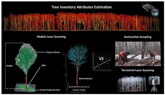
Mobile Laser Scanning for Estimating Tree Structural Attributes in a Temperate Hardwood Forest

 , ,
, ,
Abstract
:
1. Introduction
2. Materials
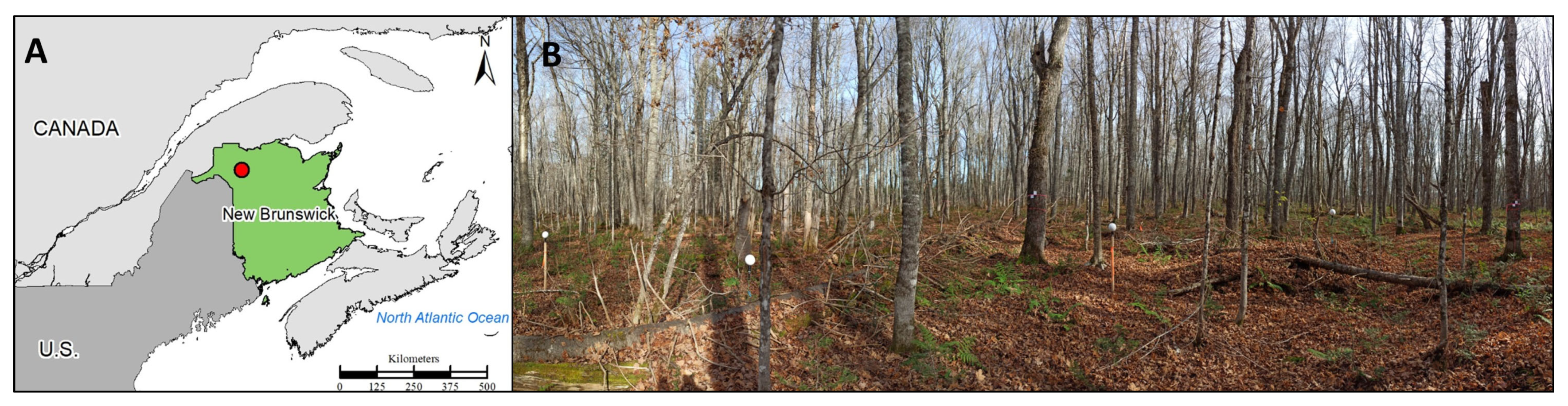
2.1. Study Site
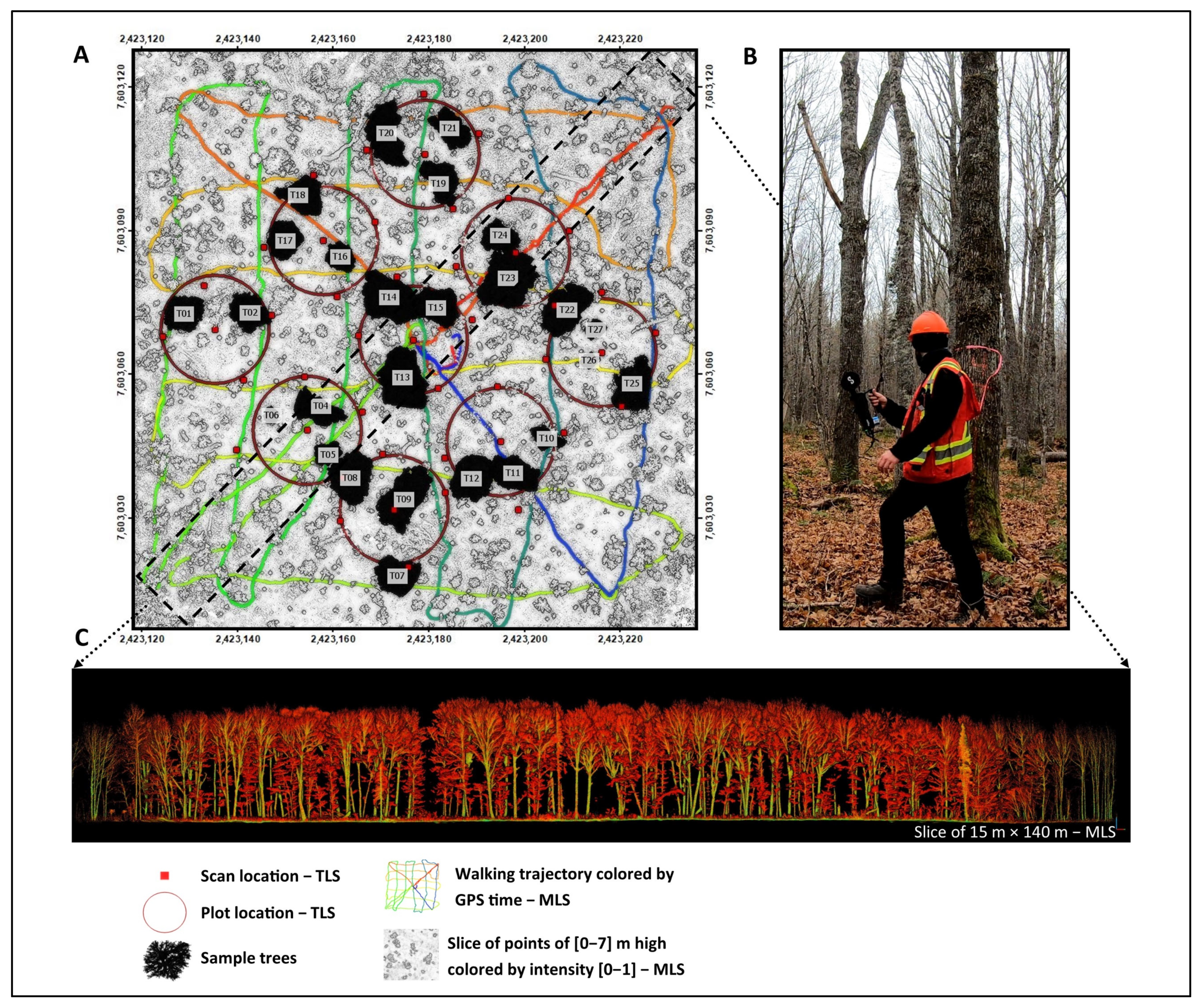
2.2. Field Measurements
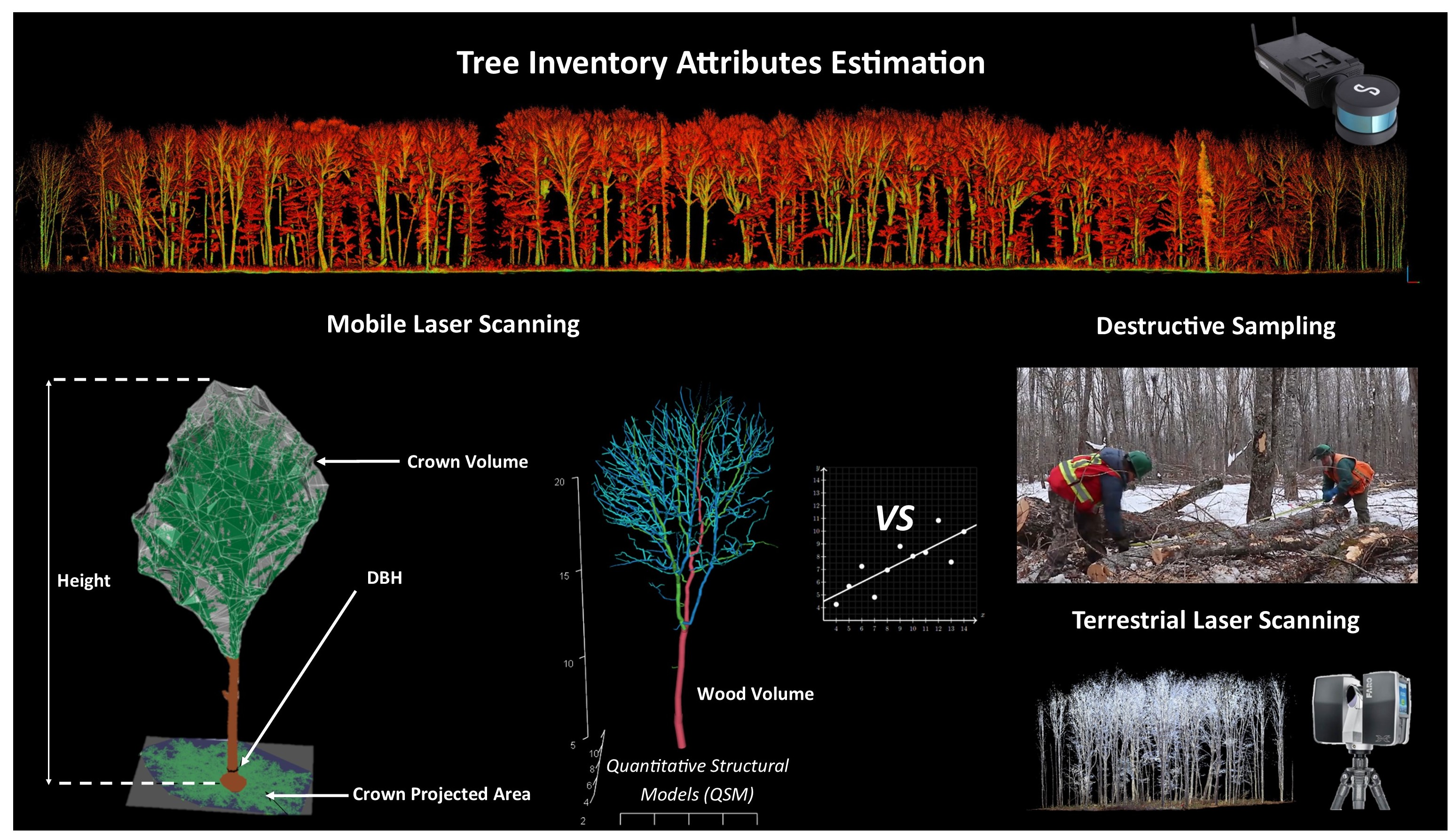
2.3. Terrestrial Laser Scanning (TLS) Data
2.4. Mobile Laser Scanning (MLS) Data
3. Methods
- Operational merchantable volume: volume of the stem and all branches of a tree, with the smallest segment being longer than 244 cm with a small end DOB ≥ 8 cm;
- Merchantable stem volume: volume of the stem, with a small end DOB ≥ 8 cm (i.e., the main stem to the top of a tree excluding branches);
- Merchantable volume: volume of the stem and all branches of a tree with a small end DOB ≥ 8 cm.
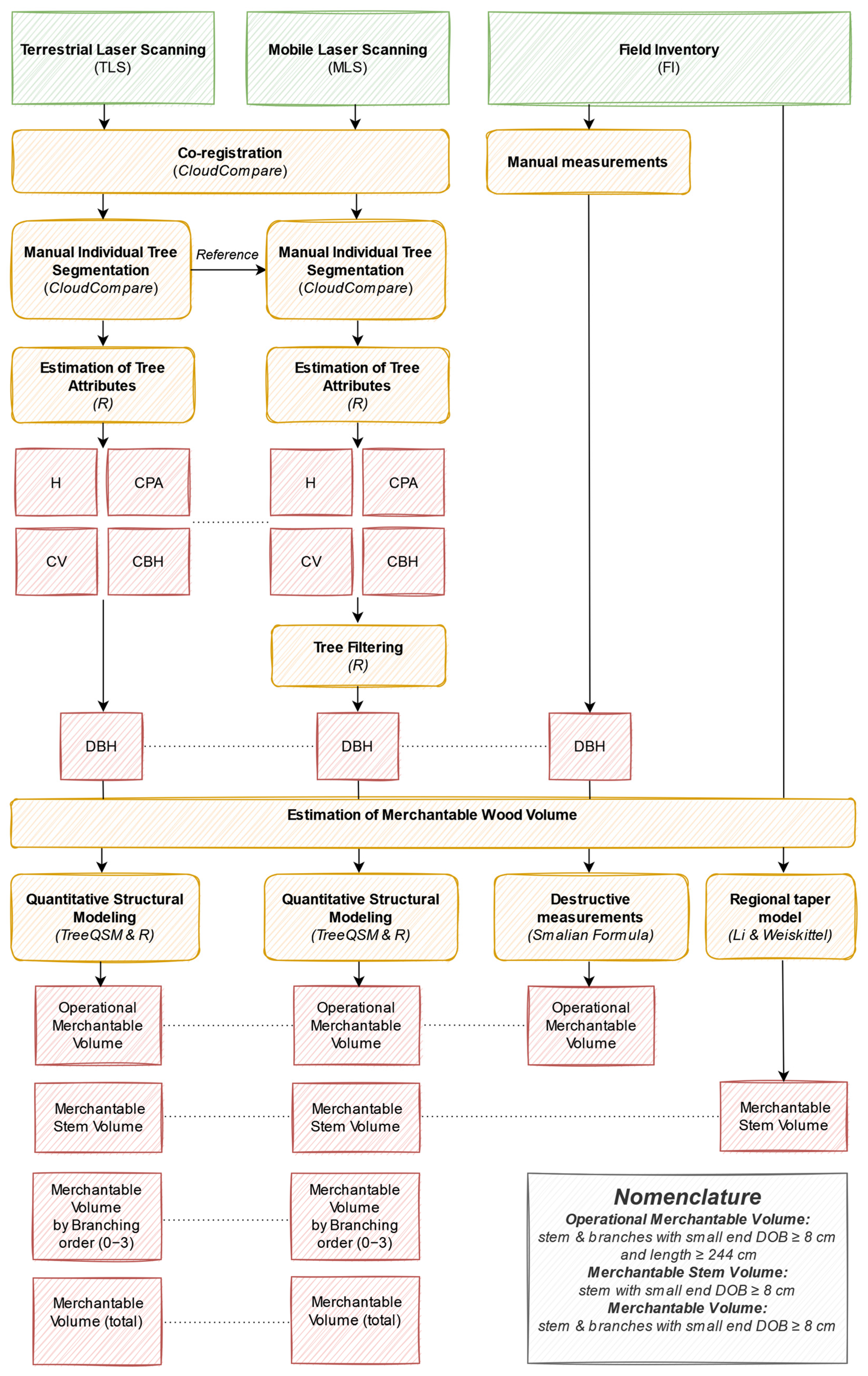
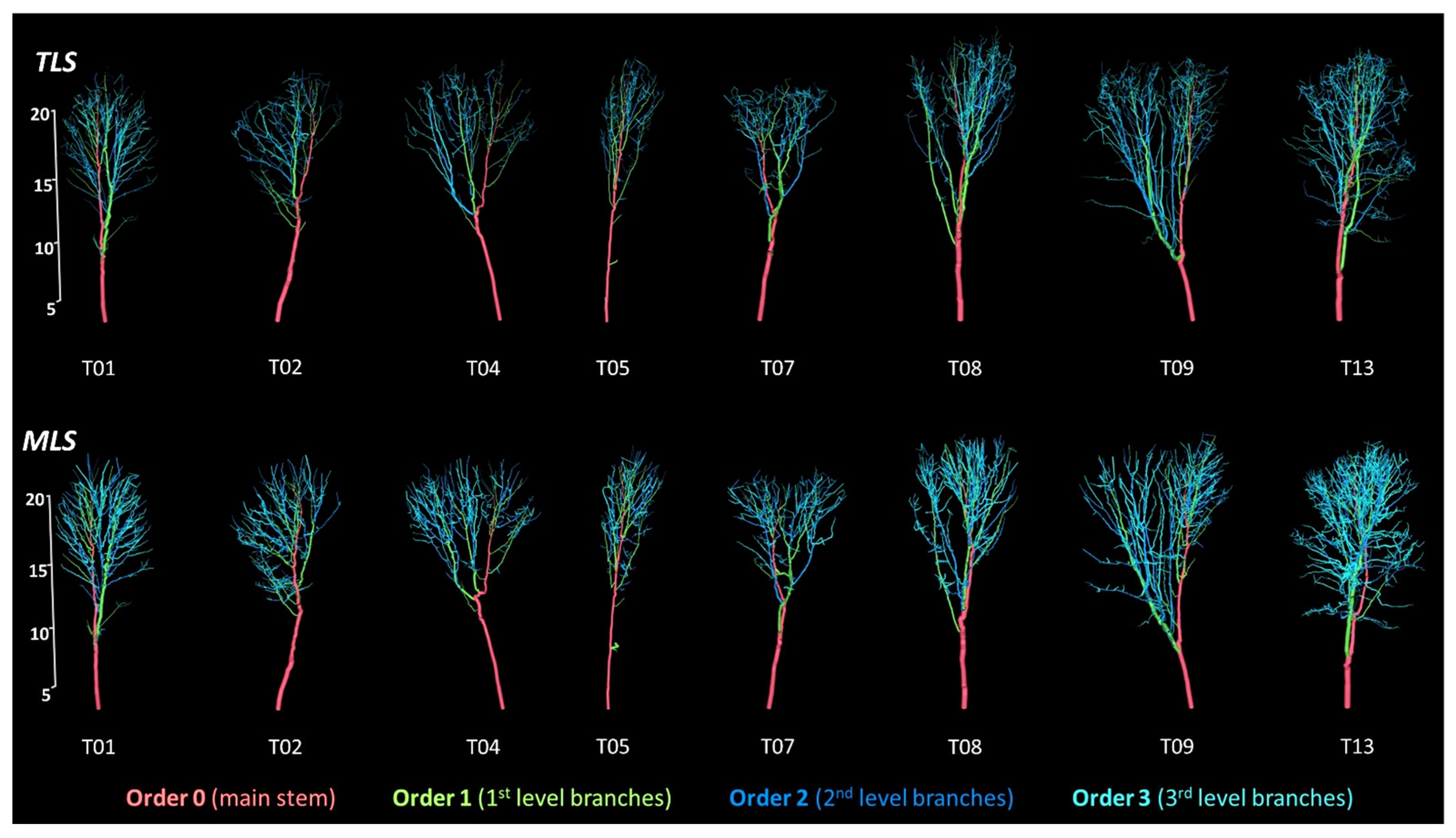
3.1. Manual Individual Tree Segmentation
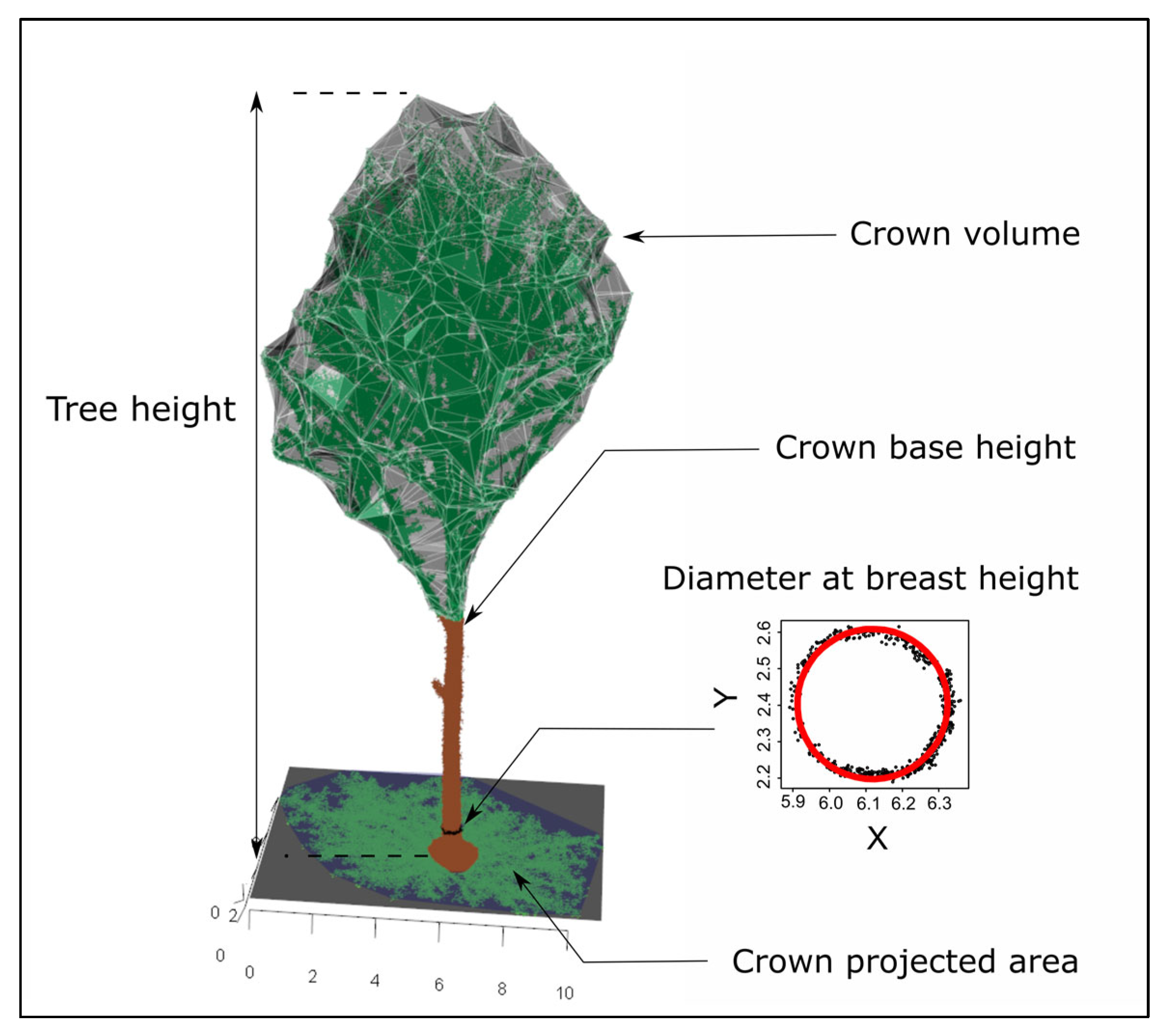
3.2. Estimation of Tree Attributes
- H was estimated as the difference between the highest and the lowest point of the manually segmented tree point cloud;
- CPA was determined using the area of the convex hull that was computed on the crown points projected in the xy-plane. The crown points are defined as the points higher than the identified CBH;
- CV was determined using an alpha shape computed on crown points (α = 1);
- DBH was estimated by fitting a circle on the XY coordinates of a 5-cm wide point cloud slice, located between 1.275 and 1.325 m height above ground, using the R package “conicfit” [35]. The ground was considered as the lowest Z coordinates of the manually segmented tree point cloud.
3.3. Estimation of Merchantable Wood Volume
3.4. Accuracy Assessment on Estimated Attributes
4. Results
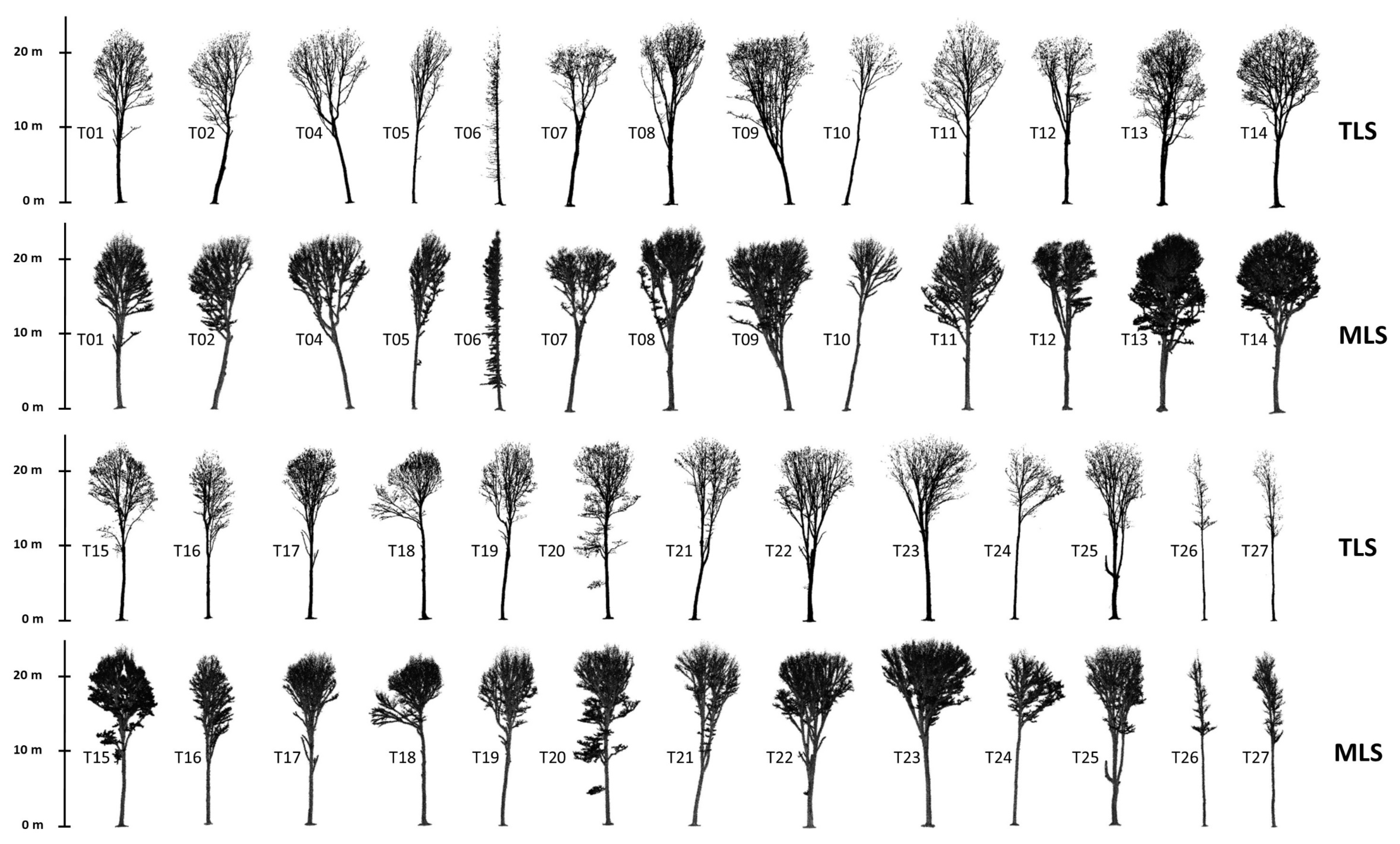
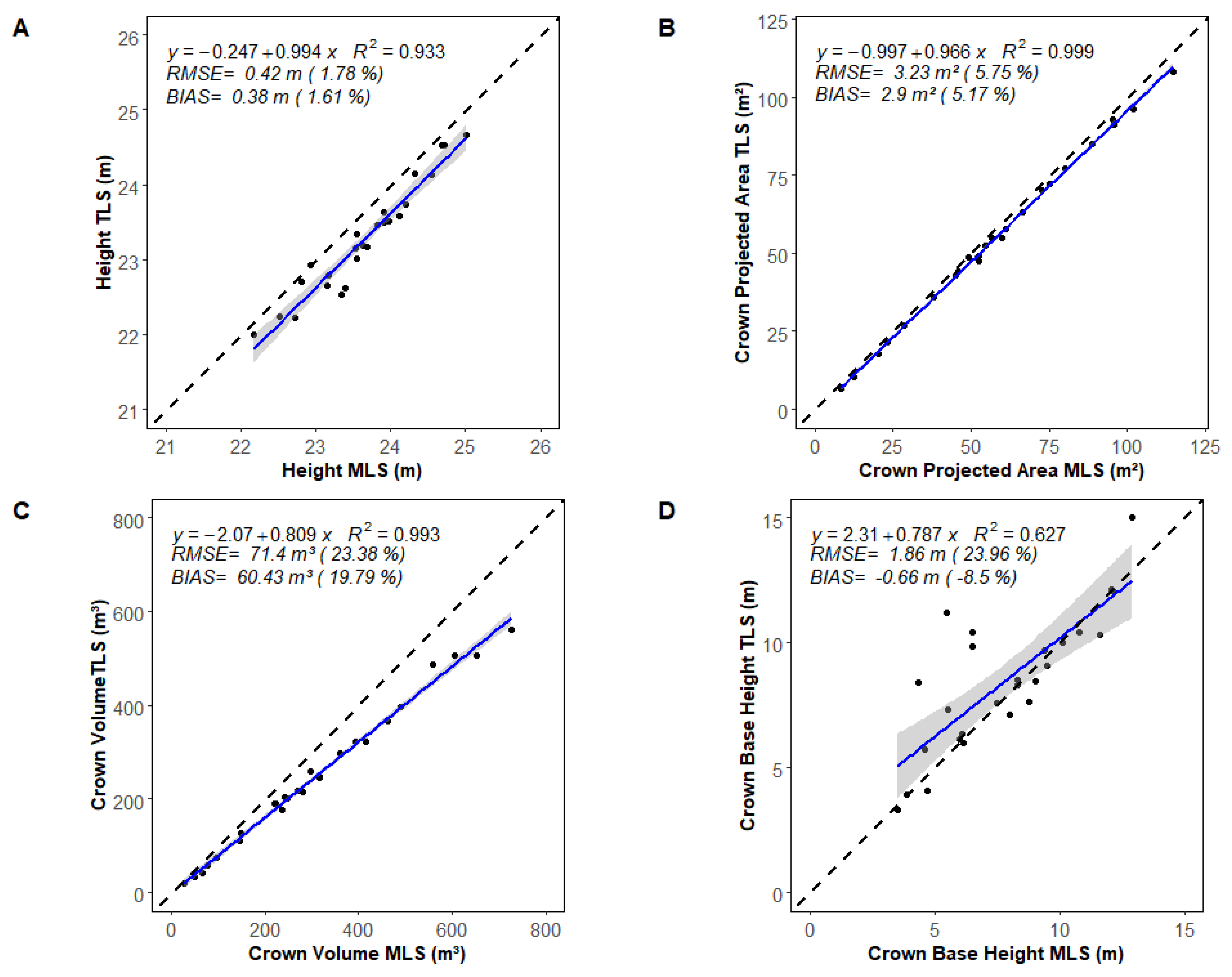
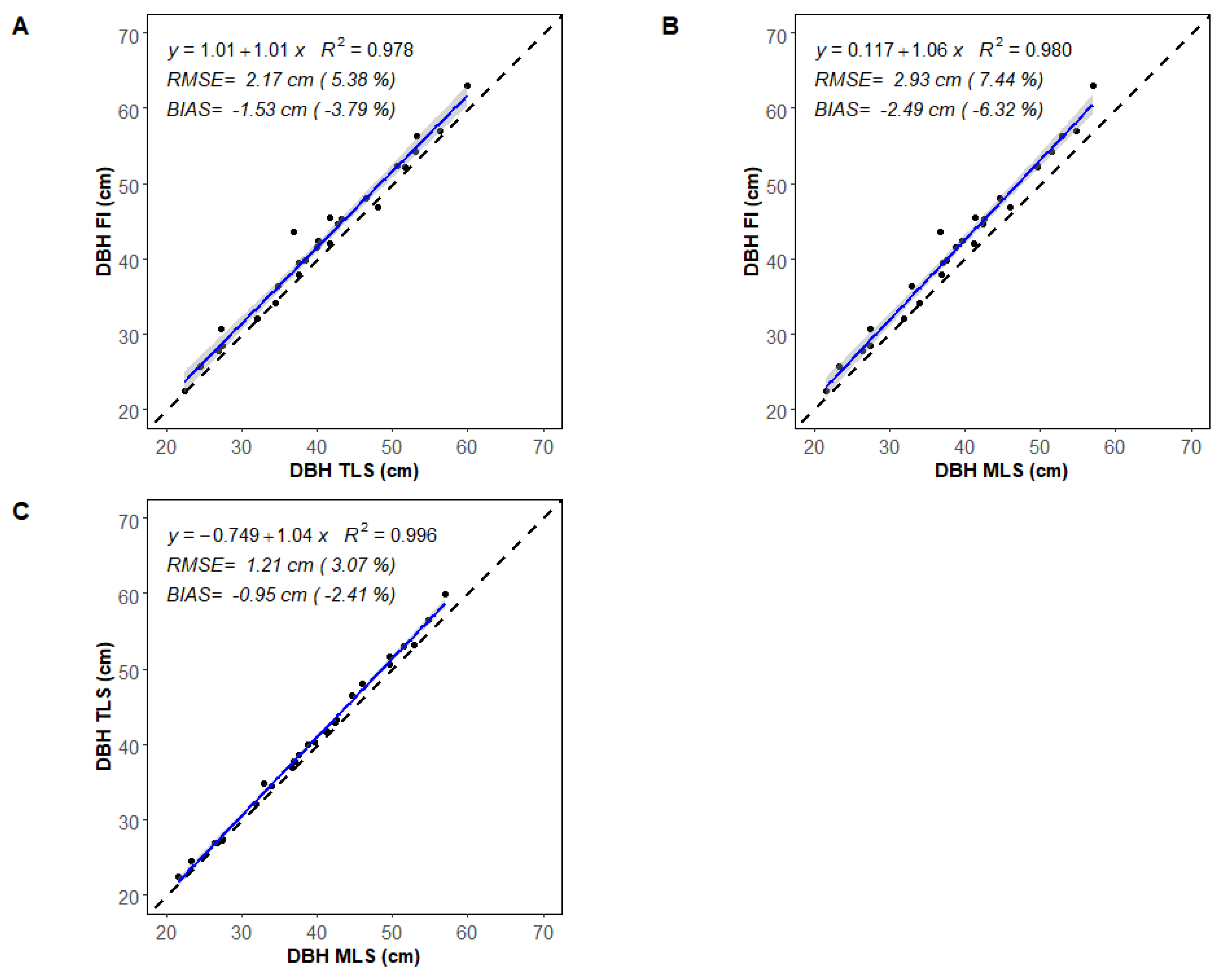
4.1. Tree Height, Crown Dimensions and DBH
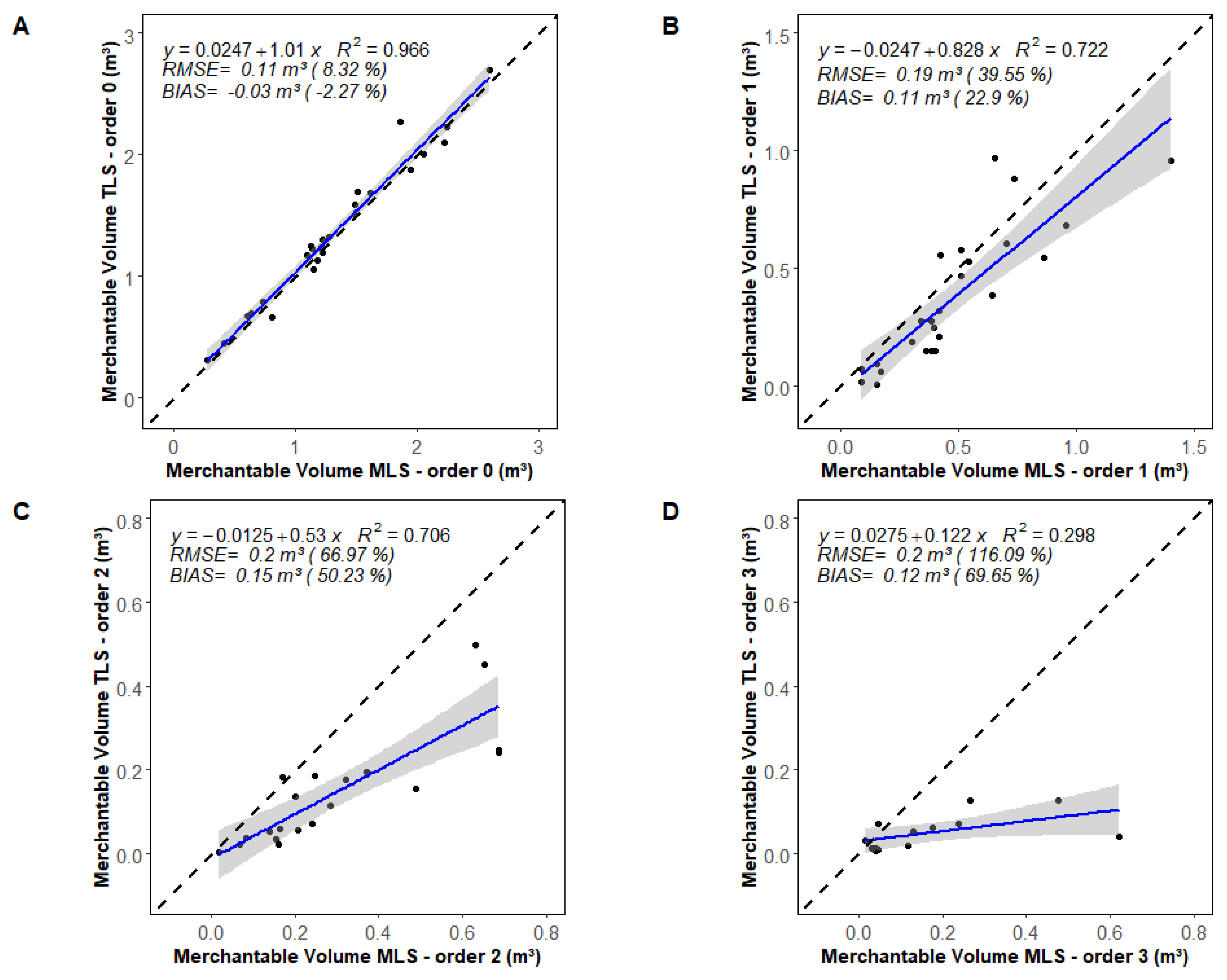
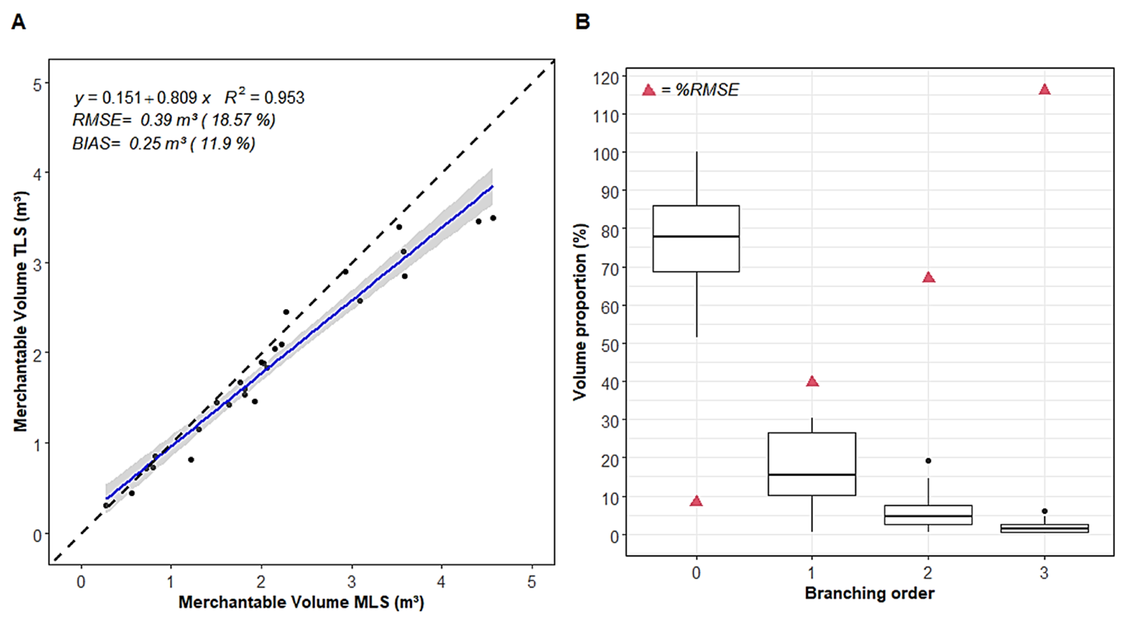
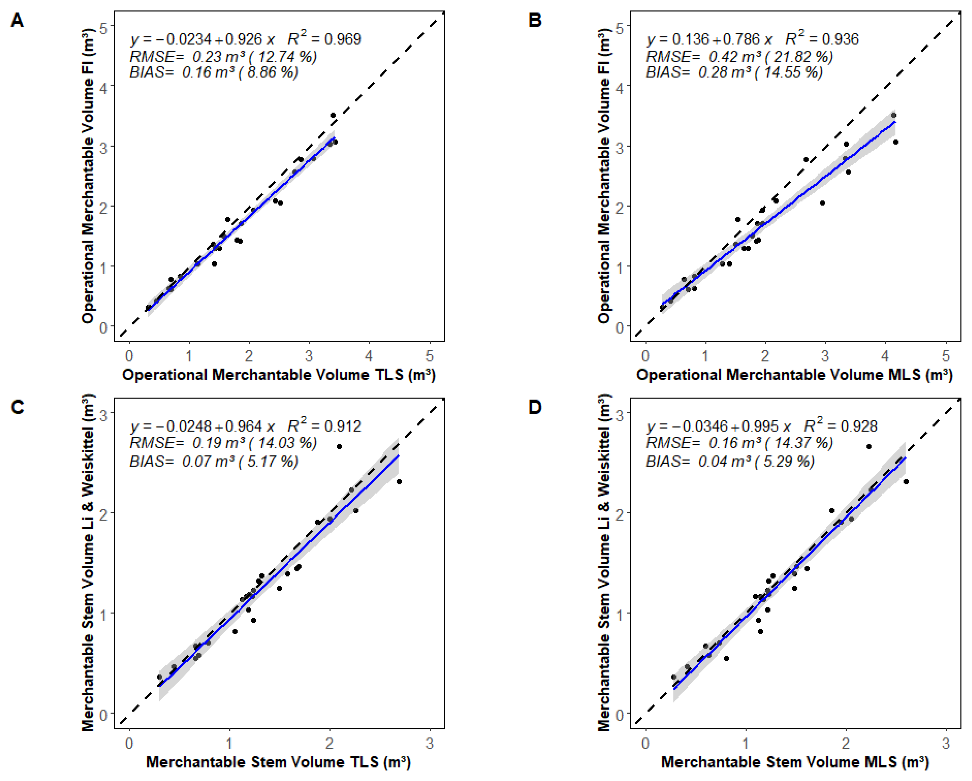
4.2. Merchantable Wood Volume (QSM)
5. Discussion
5.1. Comparison of Estimated Attributes with Past Studies
5.2. Applicability and Further Development
6. Conclusions
Author Contributions
Funding
Data Availability Statement
Acknowledgments
Conflicts of Interest
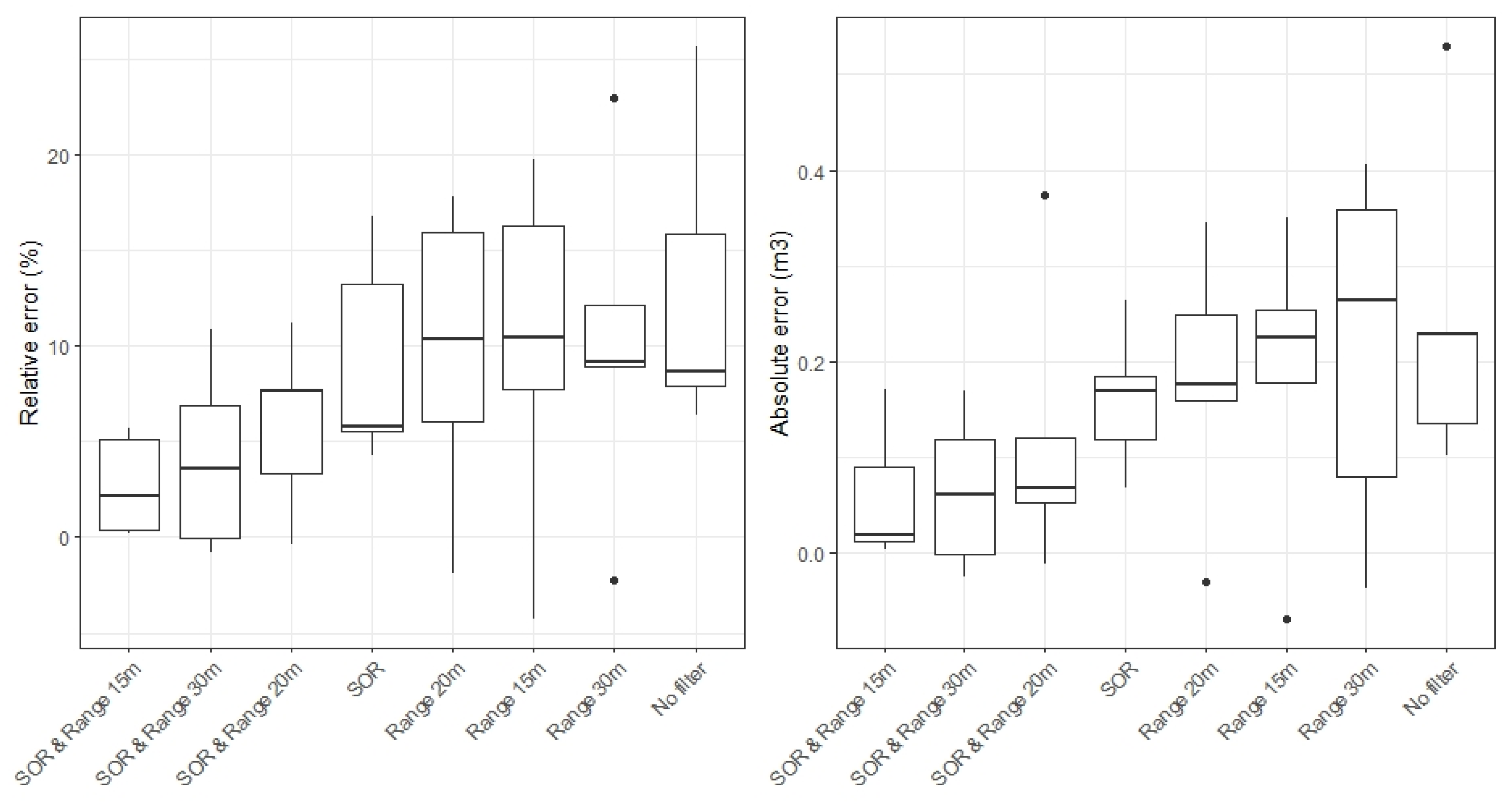
Appendix A. Point Cloud Filtering Evaluation
- No filter
- SOR filter only
- Range filter at 15 m only
- Range filter at 20 m only
- Range filter at 30 m only
- SOR + Range filter at 15 m
- SOR + Range filter at 20 m
- SOR + Range filter at 30 m

| ID | H (m) | CBH (m) | CPA (m2) | CV (m3) | DBH (cm) |
|---|---|---|---|---|---|
| T04 | 23.3 | 8.5 | 49.2 | 217 | 37.6 |
| T05 | 23.2 | 10.4 | 17.8 | 73.4 | 27.2 |
| T15 | 23.7 | 8.3 | 54.9 | 244.4 | 37.7 |
| T22 | 23.2 | 6 | 77.2 | 366.6 | 59.9 |
| T23 | 24.7 | 12.2 | 108.1 | 505.1 | 56.6 |

References
- Luoma, V.; Saarinen, N.; Wulder, M.A.; White, J.C.; Vastaranta, M.; Holopainen, M.; Hyyppä, J. Assessing Precision in Conventional Field Measurements of Individual Tree Attributes. Forests 2017, 8, 38. [Google Scholar] [CrossRef]
- Achim, A.; Moreau, G.; Coops, N.C.; Axelson, J.N.; Barrette, J.; Bédard, S.; Byrne, K.E.; Caspersen, J.; Dick, A.R.; D’Orangeville, L.; et al. The Changing Culture of Silviculture. For. Int. J. For. Res. 2021, 95, 143–152. [Google Scholar] [CrossRef]
- McRoberts, R.E.; Westfall, J.A. Effects of Uncertainty in Model Predictions of Individual Tree Volume on Large Area Volume Estimates. For. Sci. 2014, 60, 34–42. [Google Scholar] [CrossRef]
- Muukkonen, P. Generalized Allometric Volume and Biomass Equations for Some Tree Species in Europe. Eur. J. For. Res. 2007, 126, 157–166. [Google Scholar] [CrossRef]
- Forrester, D.I.; Pretzsch, H. Tamm Review: On the Strength of Evidence When Comparing Ecosystem Functions of Mixtures with Monocultures. For. Ecol. Manag. 2015, 356, 41–53. [Google Scholar] [CrossRef]
- Vorster, A.G.; Evangelista, P.H.; Stovall, A.E.L.; Ex, S. Variability and Uncertainty in Forest Biomass Estimates from the Tree to Landscape Scale: The Role of Allometric Equations. Carbon Balance Manag. 2020, 15, 8. [Google Scholar] [CrossRef]
- Calders, K.; Adams, J.; Armston, J.; Bartholomeus, H.; Bauwens, S.; Bentley, L.P.; Chave, J.; Danson, F.M.; Demol, M.; Disney, M.; et al. Terrestrial Laser Scanning in Forest Ecology: Expanding the Horizon. Remote Sens Environ. 2020, 251, 112102. [Google Scholar] [CrossRef]
- Wilkes, P.; Lau, A.; Disney, M.; Calders, K.; Burt, A.; Gonzalez de Tanago, J.; Bartholomeus, H.; Brede, B.; Herold, M. Data Acquisition Considerations for Terrestrial Laser Scanning of Forest Plots. Remote Sens Environ. 2017, 196, 140–153. [Google Scholar] [CrossRef]
- Raumonen, P.; Kaasalainen, M.; Markku, Å.; Kaasalainen, S.; Kaartinen, H.; Vastaranta, M.; Holopainen, M.; Disney, M.; Lewis, P. Fast Automatic Precision Tree Models from Terrestrial Laser Scanner Data. Remote Sens. 2013, 5, 491–520. [Google Scholar] [CrossRef]
- Hackenberg, J.; Spiecker, H.; Calders, K.; Disney, M.; Raumonen, P. SimpleTree—An Efficient Open Source Tool to Build Tree Models from TLS Clouds. Forests 2015, 6, 4245–4294. [Google Scholar] [CrossRef]
- Demol, M.; Wilkes, P.; Raumonen, P.; Krishna Moorthy, S.; Calders, K.; Gielen, B.; Verbeeck, H. Volumetric Overestimation of Small Branches in 3D Reconstructions of Fraxinus Excelsior. Silva. Fennica. 2022, 56, 1–26. [Google Scholar] [CrossRef]
- Burt, A.; Boni Vicari, M.; da Costa, A.C.L.; Coughlin, I.; Meir, P.; Rowland, L.; Disney, M. New Insights into Large Tropical Tree Mass and Structure from Direct Harvest and Terrestrial Lidar. R. Soc. Open Sci. 2021, 8, 201458. [Google Scholar] [CrossRef]
- Liang, X.; Hyyppä, J.; Kaartinen, H.; Lehtomäki, M.; Pyörälä, J.; Pfeifer, N.; Holopainen, M.; Brolly, G.; Francesco, P.; Hackenberg, J.; et al. International Benchmarking of Terrestrial Laser Scanning Approaches for Forest Inventories. ISPRS J. Photogramm. Remote Sens. 2018, 144, 137–179. [Google Scholar] [CrossRef]
- Liang, X.; Kukko, A.; Hyyppä, J.; Lehtomäki, M.; Pyörälä, J.; Yu, X.; Kaartinen, H.; Jaakkola, A.; Wang, Y. In-Situ Measurements from Mobile Platforms: An Emerging Approach to Address the Old Challenges Associated with Forest Inventories. ISPRS J. Photogramm. Remote Sens. 2018, 143, 97–107. [Google Scholar] [CrossRef]
- di Stefano, F.; Chiappini, S.; Gorreja, A.; Balestra, M.; Pierdicca, R. Mobile 3D Scan LiDAR: A Literature Review. Geomat. Nat. Hazards Risk 2021, 12, 2387–2429. [Google Scholar] [CrossRef]
- Liang, X.; Hyyppa, J.; Kukko, A.; Kaartinen, H.; Jaakkola, A.; Yu, X. The Use of a Mobile Laser Scanning System for Mapping Large Forest Plots. IEEE Geosci. Remote Sens. Lett. 2014, 11, 1504–1508. [Google Scholar] [CrossRef]
- Balenović, I.; Liang, X.; Jurjević, L.; Hyyppä, J.; Seletković, A.; Kukko, A. Hand-Held Personal Laser Scanning—Current Status and Perspectives for Forest Inventory Application. Croat. J. For. Eng. 2020, 42, 165–183. [Google Scholar] [CrossRef]
- Cabo, C.; del Pozo, S.; Rodríguez-Gonzálvez, P.; Ordóñez, C.; González-Aguilera, D. Comparing Terrestrial Laser Scanning (TLS) and Wearable Laser Scanning (WLS) for Individual Tree Modeling at Plot Level. Remote Sens. 2018, 10, 540. [Google Scholar] [CrossRef]
- Hartley, R.J.L.; Jayathunga, S.; Massam, P.D.; de Silva, D.; Estarija, H.J.; Davidson, S.J.; Wuraola, A.; Pearse, G.D. Assessing the Potential of Backpack-Mounted Mobile Laser Scanning Systems for Tree Phenotyping. Remote Sens. 2022, 14, 3344. [Google Scholar] [CrossRef]
- Donager, J.J.; Sánchez Meador, A.J.; Blackburn, R.C. Adjudicating Perspectives on Forest Structure: How Do Airborne, Terrestrial, and Mobile Lidar-Derived Estimates Compare? Remote Sens. 2021, 13, 2297. [Google Scholar] [CrossRef]
- Bauwens, S.; Bartholomeus, H.; Calders, K.; Lejeune, P. Forest Inventory with Terrestrial LiDAR: A Comparison of Static and Hand-Held Mobile Laser Scanning. Forests 2016, 7, 127. [Google Scholar] [CrossRef]
- Chen, S.; Liu, H.; Feng, Z.; Shen, C.; Chen, P. Applicability of Personal Laser Scanning in Forestry Inventory. PLoS ONE 2019, 14, e0211392. [Google Scholar] [CrossRef]
- Potter, T.L. Mobile Laser Scanning in Forests: Mapping Beneath the Canopy. Ph.D. Thesis, University of Leicester, Leicester, UK, 2019. Available online: https://leicester.figshare.com/articles/thesis/Mobile_laser_scanning_in_forests_Mapping_beneath_the_canopy/11322848 (accessed on 2 August 2022).
- Hyyppä, E.; Yu, X.; Kaartinen, H.; Hakala, T.; Kukko, A.; Vastaranta, M.; Hyyppä, J. Comparison of Backpack, Handheld, under-Canopy UAV, and above-Canopy UAV Laser Scanning for Field Reference Data Collection in Boreal Forests. Remote Sens. 2020, 12, 3327. [Google Scholar] [CrossRef]
- Arkin, J.; Coops, N.C.; Daniels, L.D.; Plowright, A. Estimation of Vertical Fuel Layers in Tree Crowns Using High Density Lidar Data. Remote Sens. 2021, 13, 4598. [Google Scholar] [CrossRef]
- Niță, M.D. Testing Forestry Digital Twinning Workflow Based on Mobile Lidar Scanner and Ai Platform. Forests 2021, 12, 1576. [Google Scholar] [CrossRef]
- Bienert, A.; Georgi, L.; Kunz, M.; von Oheimb, G.; Maas, H.G. Automatic Extraction and Measurement of Individual Trees from Mobile Laser Scanning Point Clouds of Forests. Ann. Bot. 2021, 128, 787–804. [Google Scholar] [CrossRef]
- Jin, S.; Zhang, W.; Shao, J.; Wan, P.; Cheng, S.; Cai, S.; Yan, G. Estimation of Larch Growth at the Stem, Crown and Branch Levels Using Ground-Based LiDAR Point Cloud. 2021. Available online: https://assets.researchsquare.com/files/rs-910503/v1_covered.pdf?c=1632840255 (accessed on 2 August 2022).
- Zelazny, V.F.; New Brunswick Department of Natural Resources; New Brunswick Ecosystem Classsification Working Group. Our Landscape Heritage: The Story of Ecological Land Classification in New Brunswick = Notre Patrimoine Du Paysage, l’histoire de La Classification Écologique Des Terres Au Nouveau-Brunswick; New Brunswick Dept. of Natural Resources: Fredericton, NB, Canada, 2007; ISBN 9781553962038.
- Colpitts, M.C.; Fahmy, S.H.; MacDougall, J.E.; Ng, T.T.M.; McInnis, B.G.; Zelazny, V.F. Forest Soils of New Brunswick. CLBRR contribution No. 95-38; U.S. Department of Energy, Office of Scientific and Technical Information: Oak Ridge, TN, USA, 1995. [Google Scholar]
- Vandendaele, B.; Fournier, R.A.; Vepakomma, U.; Pelletier, G.; Lejeune, P.; Martin-ducup, O. Estimation of Northern Hardwood Forest Inventory Attributes Using Uav Laser Scanning (Uls): Transferability of Laser Scanning Methods and Comparison of Automated Approaches at the Tree- and Stand-level. Remote Sens. 2021, 13, 2796. [Google Scholar] [CrossRef]
- CloudCompare, Version 2.11.3. GPL Software. 2020. Available online: http://www.Cloudcompare.Org/(accessed on 20 December 2021).
- R Core Team. R: A Language and Environment for Statistical Computing; R Foundation for Statistical Computing: Vienna, Austria, 2017; Available online: https://www.R-Project.Org/ (accessed on 20 December 2021).
- Schneider, R.; Calama, R.; Martin-Ducup, O. Understanding Tree-to-Tree Variations in Stone Pine (Pinus Pinea l.) Cone Production Using Terrestrial Laser Scanner. Remote Sens. 2020, 12, 173. [Google Scholar] [CrossRef]
- Gama, J.; Chernov, N. Conicfit: Algorithms for Fitting Circles, Ellipses and Conics Based on the Work by Prof. Nikolai Chernov. R Package Version 1.0.4. 2015. Available online: https://CRAN.R-Project.Org/Package=conicfit (accessed on 15 April 2022).
- Lecigne, B.; Delagrange, S.; Messier, C. Exploring Trees in Three Dimensions: VoxR, a Novel Voxel-Based R Package Dedicated to Analysing the Complex Arrangement of Tree Crowns. Ann. Bot. 2018, 121, 589–601. [Google Scholar] [CrossRef]
- Martin-Ducup, O.; Mofack, G.; Wang, D.; Raumonen, P.; Ploton, P.; Sonké, B.; Barbier, N.; Couteron, P.; Pélissier, R. Evaluation of Automated Pipelines for Tree and Plot Metric Estimation from TLS Data in Tropical Forest Areas. Ann. Bot. 2021, 128, 753–766. [Google Scholar] [CrossRef] [PubMed]
- Martin-Ducup, O.; Lecigne, B. ARchi: Quantitative Structural Model (‘QSM’) Treatment for Tree Architecture. R Package Version 2.1.0. Available online: https://CRAN.R-Project.Org/Package=aRchi (accessed on 20 April 2022).
- Li, R.; Weiskittel, A.; Dick, A.R.; Kershaw, J.A.; Seymour, R.S. Regional Stem Taper Equations for Eleven Conifer Species in the Acadian Region of North America: Development and Assessment. North. J. Appl. For. 2012, 29, 5–14. [Google Scholar] [CrossRef]
- Weiskittel, A.; Li, R. Development of Regional Taper and Volume Equations: Hardwood Species; DendroMetrics, LLC: Welches, OR, USA, 2012. [Google Scholar]
- Bruce, D.; Schumacher, F.X. Forest Mensuration; McGraw-Hill: New York, NY, USA, 1950. [Google Scholar]
- Gollob, C.; Ritter, T.; Nothdurft, A. Forest Inventory with Long Range and High-Speed Personal Laser Scanning (PLS) and Simultaneous Localization and Mapping (SLAM) Technology. Remote Sens. 2020, 12, 1509. [Google Scholar] [CrossRef]
- del Perugia, B.; Giannetti, F.; Chirici, G.; Travaglini, D. Influence of Scan Density on the Estimation of Single-Tree Attributes by Hand-Held Mobile Laser Scanning. Forests 2019, 10, 277. [Google Scholar] [CrossRef]
- Oveland, I.; Hauglin, M.; Gobakken, T.; Næsset, E.; Maalen-Johansen, I. Automatic Estimation of Tree Position and Stem Diameter Using a Moving Terrestrial Laser Scanner. Remote Sens. 2017, 9, 350. [Google Scholar] [CrossRef]
- Witzmann, S.; Matitz, L.; Gollob, C.; Ritter, T.; Kraßnitzer, R.; Tockner, A.; Stampfer, K.; Nothdurft, A. Accuracy and Precision of Stem Cross-Section Modeling in 3D Point Clouds from TLS and Caliper Measurements for Basal Area Estimation. Remote Sens. 2022, 14, 1923. [Google Scholar] [CrossRef]
- Giannetti, F.; Puletti, N.; Quatrini, V.; Travaglini, D.; Bottalico, F.; Corona, P.; Chirici, G. Integrating Terrestrial and Airborne Laser Scanning for the Assessment of Single-Tree Attributes in Mediterranean Forest Stands. Eur. J. Remote Sens. 2018, 51, 795–807. [Google Scholar] [CrossRef]
- Jurjević, L.; Liang, X.; Gašparović, M.; Balenović, I. Is Field-Measured Tree Height as Reliable as Believed—Part II, A Comparison Study of Tree Height Estimates from Conventional Field Measurement and Low-Cost Close-Range Remote Sensing in a Deciduous Forest. ISPRS J. Photogramm. Remote Sens. 2020, 169, 227–241. [Google Scholar] [CrossRef]
- Hyyppä, E.; Kukko, A.; Kaijaluoto, R.; White, J.C.; Wulder, M.A.; Pyörälä, J.; Liang, X.; Yu, X.; Wang, Y.; Kaartinen, H.; et al. Accurate Derivation of Stem Curve and Volume Using Backpack Mobile Laser Scanning. ISPRS J. Photogramm. Remote Sens. 2020, 161, 246–262. [Google Scholar] [CrossRef]
- Bienert, A.; Georgi, L.; Kunz, M.; Maas, H.G.; von Oheimb, G. Comparison and Combination of Mobile and Terrestrial Laser Scanning for Natural Forest Inventories. Forests 2018, 8, 395. [Google Scholar] [CrossRef]
- Demol, M.; Calders, K.; Verbeeck, H.; Gielen, B. Forest Above-Ground Volume Assessments with Terrestrial Laser Scanning: A Ground-Truth Validation Experiment in Temperate, Managed Forests. Ann. Bot. 2021, 128, 805–819. [Google Scholar] [CrossRef]
- Abegg, M.; Boesch, R.; Schaepman, M.E.; Morsdorf, F. Impact of Beam Diameter and Scanning Approach on Point Cloud Quality of Terrestrial Laser Scanning in Forests. IEEE Trans. Geosci. Remote Sens. 2021, 59, 8153–8167. [Google Scholar] [CrossRef]
- Åkerblom, M.; Kaitaniemi, P. Terrestrial Laser Scanning: A New Standard of Forest Measuring and Modelling? Ann. Bot. 2021, 128, 653–662. [Google Scholar] [CrossRef]
- Vaaja, M.T.; Virtanen, J.-P.; Kurkela, M.; Lehtola, V.; Hyyppä, J.; Hyyppä, H. The Effect of Wind on Tree Stem Parameter Estimation Using Terrestrial Laser Scanning. ISPRS Ann. Photogramm. Remote Sens. Spat. Inf. Sci. 2016, III-8, 117–122. [Google Scholar] [CrossRef]
- Du, S.; Lindenbergh, R.; Ledoux, H.; Stoter, J.; Nan, L. AdTree: Accurate, Detailed, and Automatic Modelling of Laser-Scanned Trees. Remote Sens. 2019, 11, 2074. [Google Scholar] [CrossRef] [Green Version]


Publisher’s Note: MDPI stays neutral with regard to jurisdictional claims in published maps and institutional affiliations. |
© 2022 by the authors. Licensee MDPI, Basel, Switzerland. This article is an open access article distributed under the terms and conditions of the Creative Commons Attribution (CC BY) license (https://creativecommons.org/licenses/by/4.0/).
Share and Cite
Vandendaele, B.; Martin-Ducup, O.; Fournier, R.A.; Pelletier, G.; Lejeune, P. Mobile Laser Scanning for Estimating Tree Structural Attributes in a Temperate Hardwood Forest. Remote Sens. 2022, 14, 4522. https://doi.org/10.3390/rs14184522
Vandendaele B, Martin-Ducup O, Fournier RA, Pelletier G, Lejeune P. Mobile Laser Scanning for Estimating Tree Structural Attributes in a Temperate Hardwood Forest. Remote Sensing. 2022; 14(18):4522. https://doi.org/10.3390/rs14184522
Chicago/Turabian StyleVandendaele, Bastien, Olivier Martin-Ducup, Richard A. Fournier, Gaetan Pelletier, and Philippe Lejeune. 2022. "Mobile Laser Scanning for Estimating Tree Structural Attributes in a Temperate Hardwood Forest" Remote Sensing 14, no. 18: 4522. https://doi.org/10.3390/rs14184522
APA StyleVandendaele, B., Martin-Ducup, O., Fournier, R. A., Pelletier, G., & Lejeune, P. (2022). Mobile Laser Scanning for Estimating Tree Structural Attributes in a Temperate Hardwood Forest. Remote Sensing, 14(18), 4522. https://doi.org/10.3390/rs14184522