


A Novel Knowledge Distillation Method for Self-Supervised Hyperspectral Image Classification


Abstract
:
1. Introduction
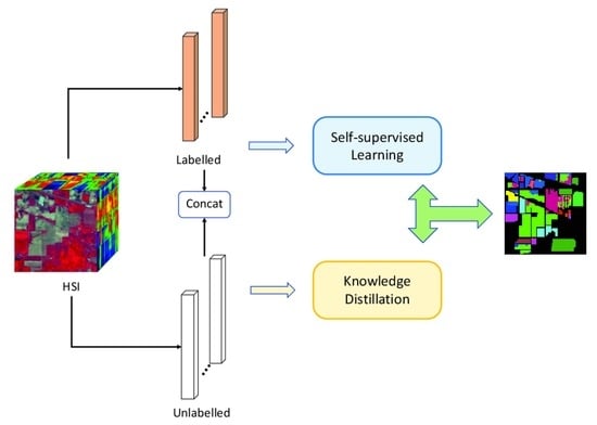
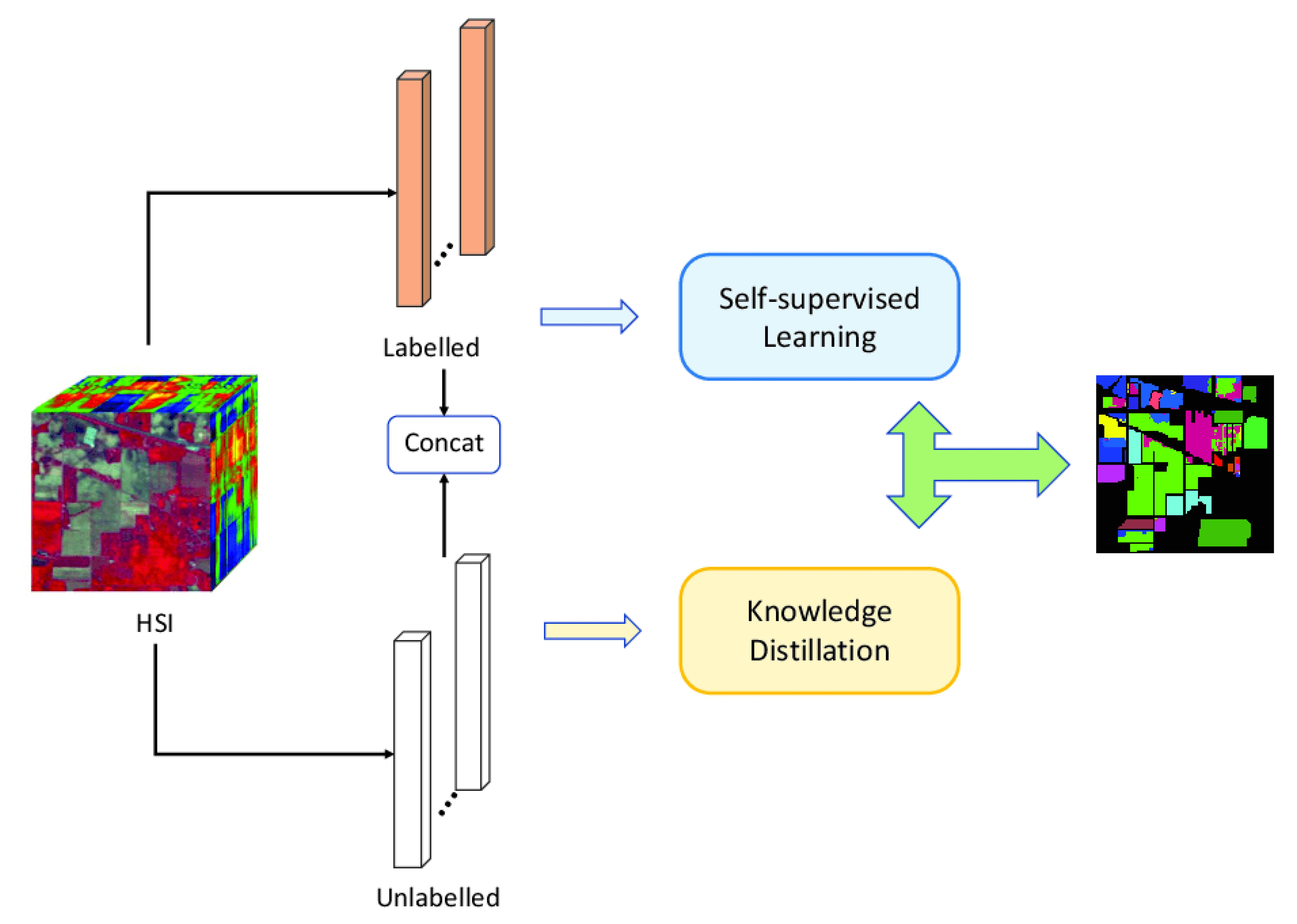
- A novel deep-learning method SSKD with combined knowledge distillation and self-supervised learning is proposed to achieve HSI classification in an end-to-end way with only a small number of labeled samples;
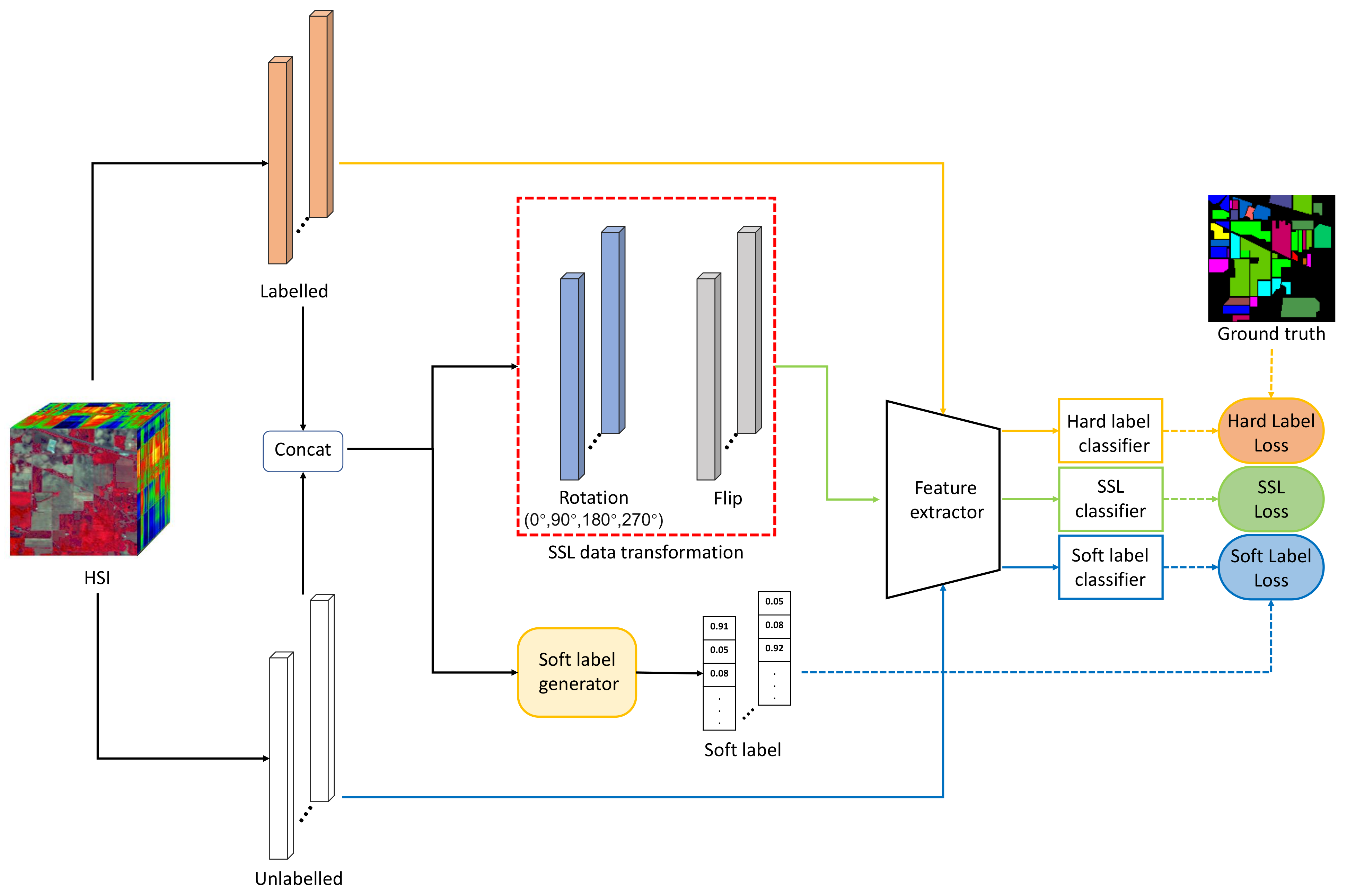
- A novel adaptive soft label generation method is proposed, in which the similarity between labeled and unlabeled samples is first calculated from spectral and spatial perspectives, and then the nearest-neighbour distance ratio between labeled and unlabeled samples is calculated to filter the available samples. The proposed adaptive soft label generation achieves a significant improvement in classification accuracy compared to state-of-the-art methods;
- We present the first concept of soft label quality in the hyperspectrum and provide a simple measure of soft label quality, the idea being to generate soft label quality by using the soft label generation algorithm for existing labeled samples and measuring it by combining the sample labels.
2. Materials and Methods
2.1. Related Work
2.1.1. Self-Supervised Learning
2.1.2. Knowledge Distillation
2.2. Methodology
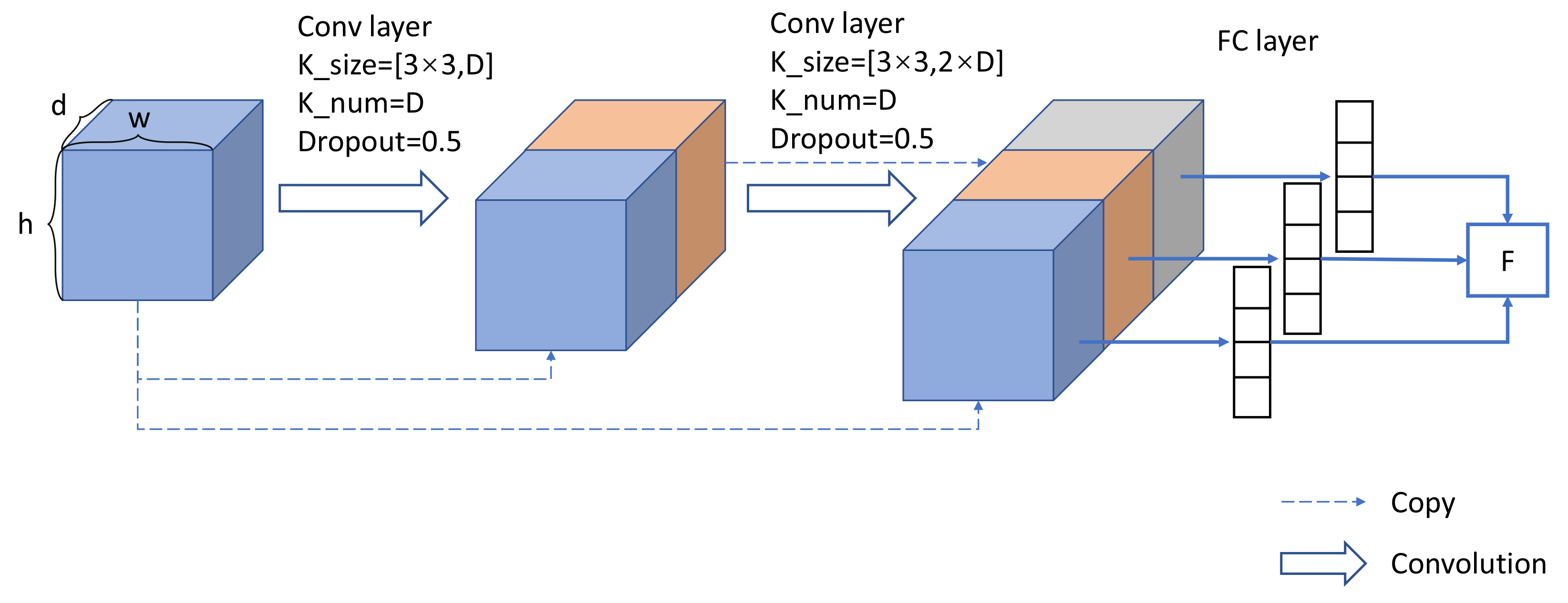
2.2.1. Self-Supervised Learning Network
2.2.2. Soft Label Generation
2.2.3. Knowledge Distillation
3. Results
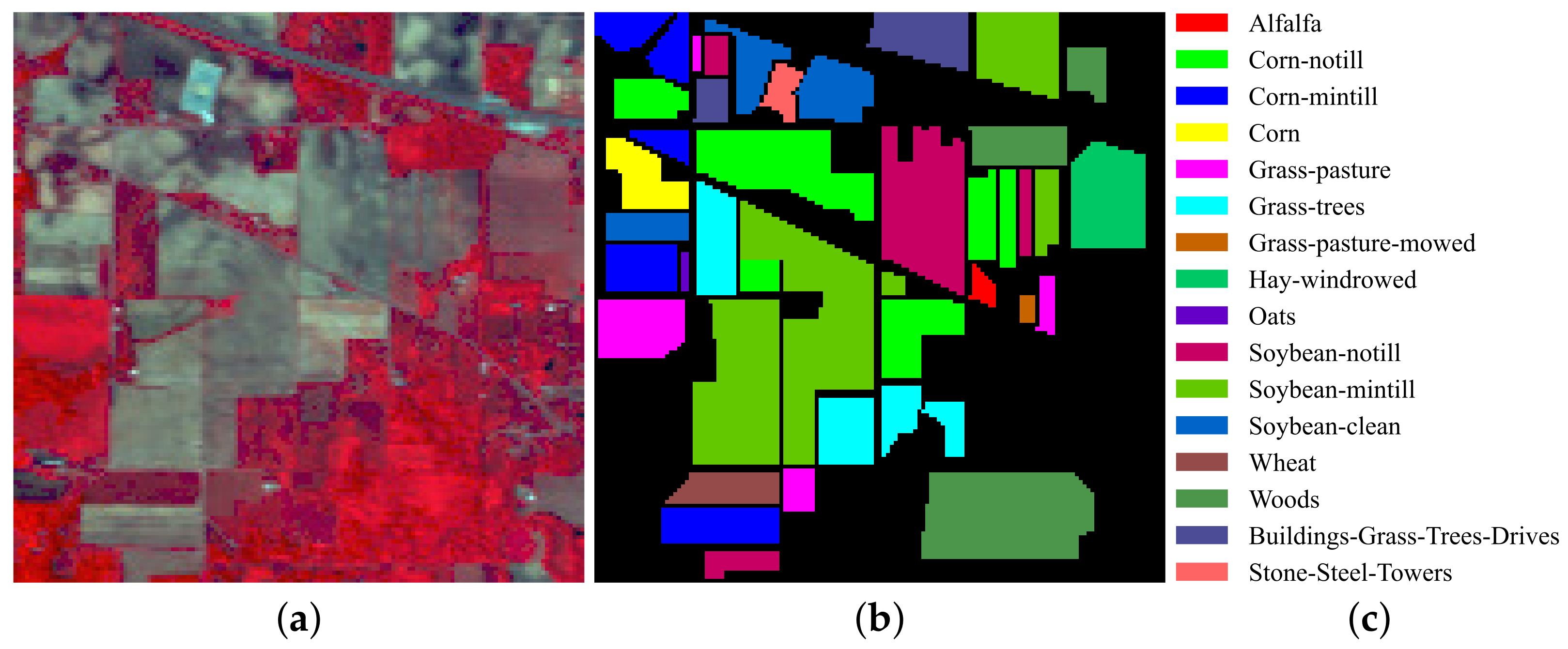
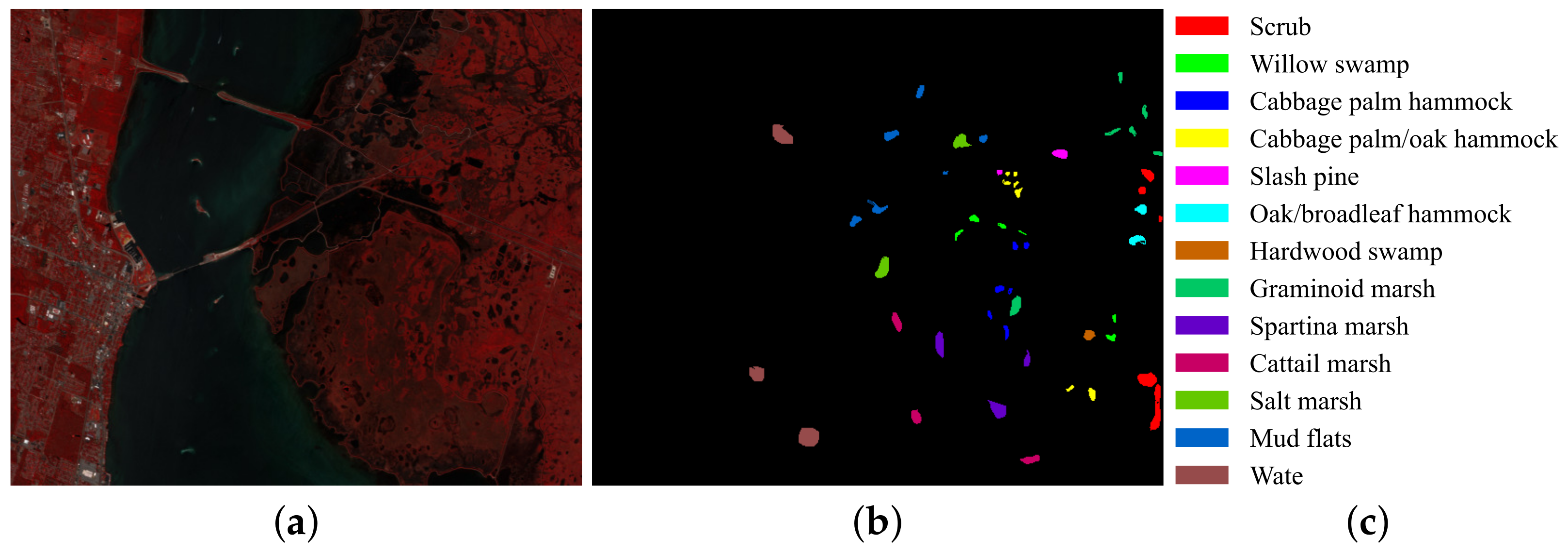
3.1. Datasets
3.2. Experimental Setup
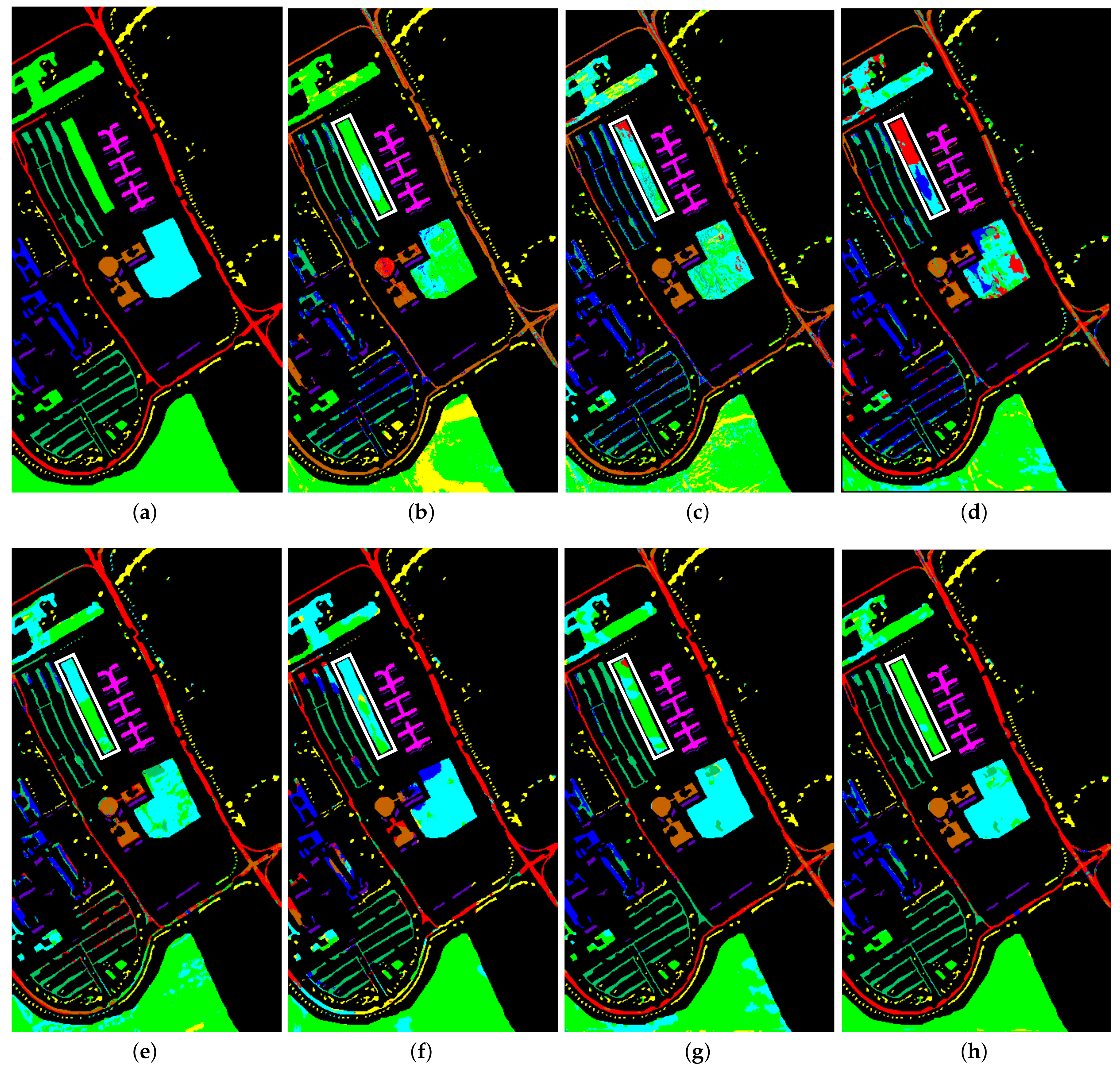
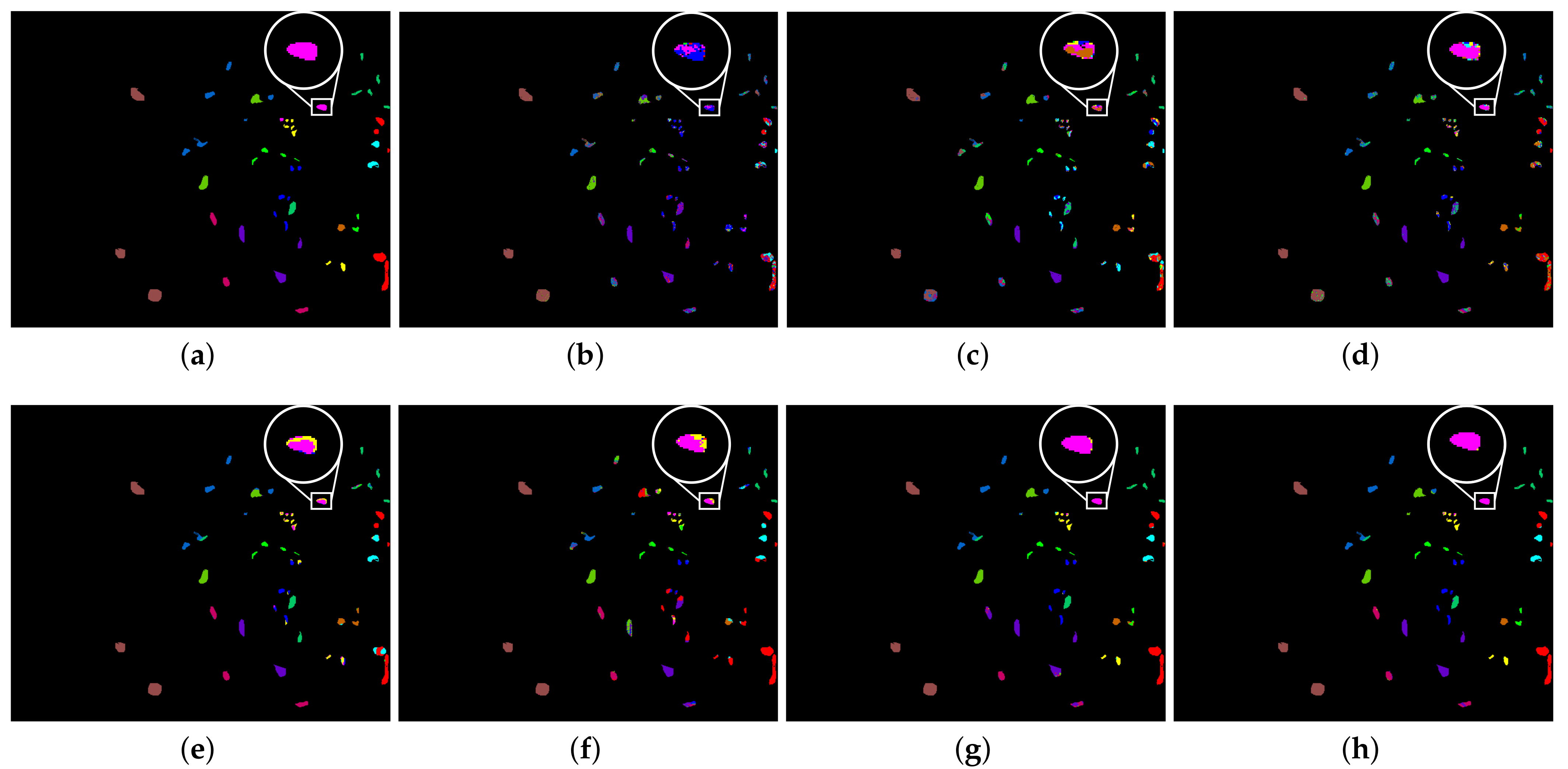
3.3. Classification Maps and Categorized Results
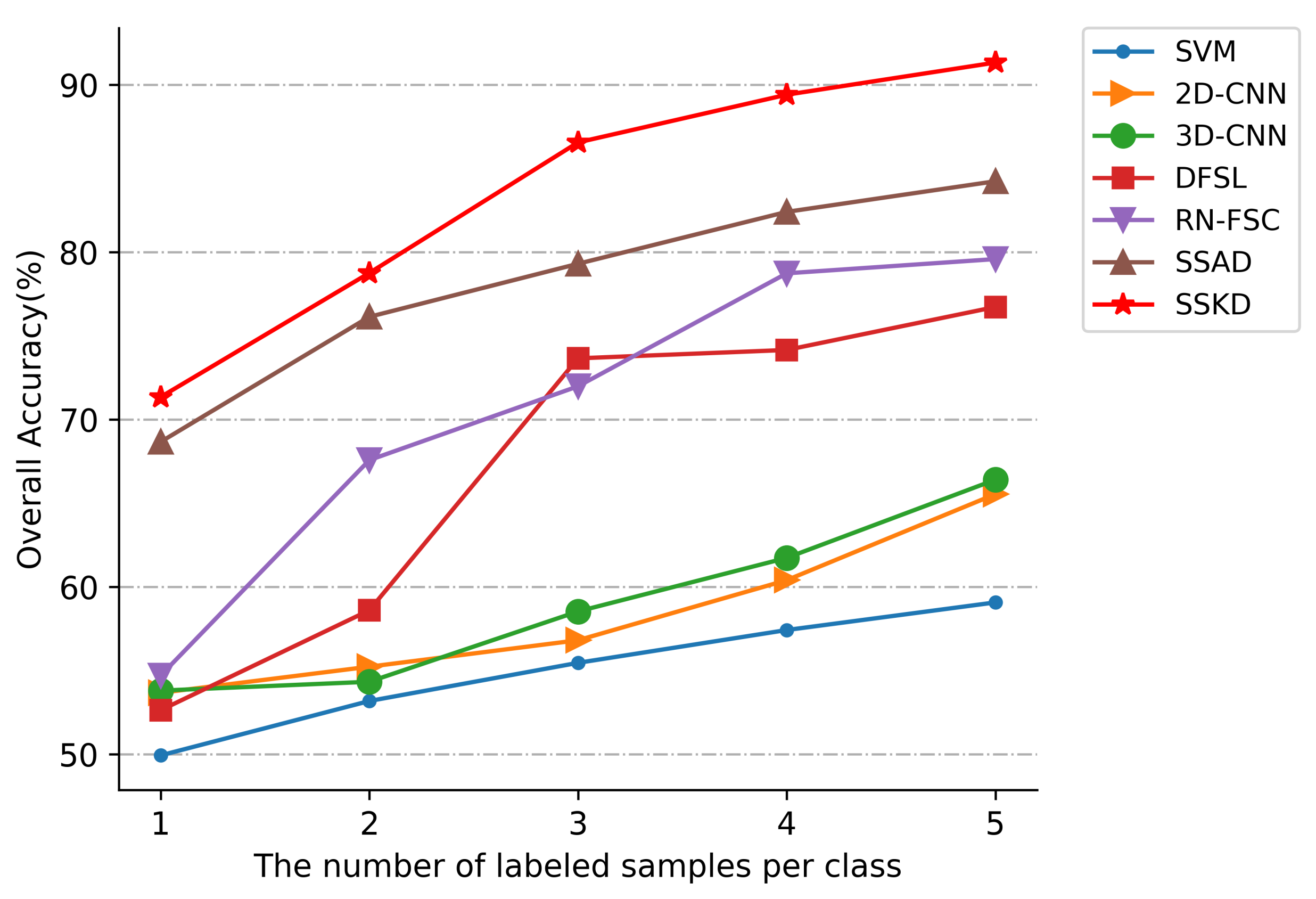
3.4. Compared with Different Number of Training Samples
3.5. Ablation Study
3.6. Efficiency Comparison
4. Discussion
- (1)
- Deep-learning methods 2DCNN and 3DCNN always outperform the traditional methods SVM. Traditional methods of SVM are limited by the inherently shallow structure of the image, making it difficult to extract deeper features. Deep learning can extract deeper image discriminative features through deep neural networks, which can achieve better classification performance. For example, the deep-learning methods 2DCNN and 3DCNN improved the overall accuracy over SVM by 6.5% and 7.33%, respectively, in the UP dataset.
- (2)
- The deep-learning approaches 2DCNN and 3DCNN achieved better classification results on all three datasets compared to the few-shot-learning-based approaches DFSL and RN-FSC. The deep-learning methods (2DCNN, 3DCNN) require a high number of training samples, so they do not perform well with only a few samples. The few-shot-learning approaches enable the models to acquire transferable visual analysis abilities by using a meta-learning training strategy, which allows the models to perform better than the general deep network models when only a small number of labeled samples are provided.
- (3)
- The approaches using soft label SSAD and SSKD performed better overall compared to the traditional methods SVM, deep-learning methods (2DCNN, 3DCNN), and few-shot-learning approaches. With only a small number of labeled samples, the previous methods only utilize a limited number of labeled samples, ignoring the problem of unlabeled sample utilization. The SSAD and SSKD, on the other hand, generate soft labels for the unlabeled samples and feed them into the network for training, fully exploiting the information contained in the unlabeled samples. The actual number of samples used is higher than other deep-learning approaches, allowing the model to extract more discriminative features from the images and achieve better classification results. The problem of a limited number of samples is overcome effectively.
- (4)
- The proposed method SSKD outperformed SSAD on the three test datasets. In terms of overall accuracy, the performance was improved by 4.88%, 7.09% and 4.96% on the three test datasets, respectively. The SSKD outperforms the SSAD in terms of the number and accuracy of soft labels generated, so the SSKD can use more unlabeled samples to train the network and can achieve efficient classification with a limited number of samples.
5. Conclusions
Author Contributions
Funding
Data Availability Statement
Conflicts of Interest
References
- Audebert, N.; Le Saux, B.; Lefèvre, S. Deep learning for classification of hyperspectral data: A comparative review. IEEE Geosci. Remote Sens. Mag. 2019, 7, 159–173. [Google Scholar] [CrossRef]
- Bioucas-Dias, J.M.; Plaza, A.; Camps-Valls, G.; Scheunders, P.; Nasrabadi, N.; Chanussot, J. Hyperspectral remote sensing data analysis and future challenges. IEEE Geosci. Remote Sens. Mag. 2013, 1, 6–36. [Google Scholar] [CrossRef]
- Jänicke, C.; Okujeni, A.; Cooper, S.; Clark, M.; Hostert, P.; van der Linden, S. Brightness gradient-corrected hyperspectral image mosaics for fractional vegetation cover mapping in northern California. Remote Sens. Lett. 2020, 11, 1–10. [Google Scholar] [CrossRef]
- Ozdemir, A.; Polat, K. Deep learning applications for hyperspectral imaging: A systematic review. J. Inst. Electron. Comput. 2020, 2, 39–56. [Google Scholar] [CrossRef]
- Yue, J.; Fang, L.; Rahmani, H.; Ghamisi, P. Self-supervised learning with adaptive distillation for hyperspectral image classification. IEEE Trans. Geosci. Remote Sens. 2021, 60, 1–13. [Google Scholar] [CrossRef]
- Jia, S.; Jiang, S.; Lin, Z.; Li, N.; Xu, M.; Yu, S. A survey: Deep learning for hyperspectral image classification with few labeled samples. Neurocomputing 2021, 448, 179–204. [Google Scholar] [CrossRef]
- Jiang, J.; Ma, J.; Chen, C.; Wang, Z.; Cai, Z.; Wang, L. SuperPCA: A superpixelwise PCA approach for unsupervised feature extraction of hyperspectral imagery. IEEE Trans. Geosci. Remote Sens. 2018, 56, 4581–4593. [Google Scholar] [CrossRef]
- Ahmad, M.; Shabbir, S.; Roy, S.K.; Hong, D.; Wu, X.; Yao, J.; Khan, A.M.; Mazzara, M.; Distefano, S.; Chanussot, J. Hyperspectral image classification—Traditional to deep models: A survey for future prospects. IEEE J. Sel. Top. Appl. Earth Observ. Remote Sens. 2021, 15, 968–999. [Google Scholar] [CrossRef]
- Licciardi, G.; Marpu, P.R.; Chanussot, J.; Benediktsson, J.A. Linear versus nonlinear PCA for the classification of hyperspectral data based on the extended morphological profiles. IEEE Geosci. Remote Sens. Lett. 2011, 9, 447–451. [Google Scholar] [CrossRef]
- Green, A.A.; Berman, M.; Switzer, P.; Craig, M.D. A transformation for ordering multispectral data in terms of image quality with implications for noise removal. IEEE Trans. Geosci. Remote Sens. 1988, 26, 65–74. [Google Scholar] [CrossRef] [Green Version]
- Hyvärinen, A.; Oja, E. Independent component analysis: Algorithms and applications. Neural Netw. 2000, 13, 411–430. [Google Scholar] [CrossRef]
- Melgani, F.; Bruzzone, L. Classification of hyperspectral remote sensing images with support vector machines. IEEE Trans. Geosci. Remote Sens. 2004, 42, 1778–1790. [Google Scholar] [CrossRef]
- Guo, Y.; Han, S.; Li, Y.; Zhang, C.; Bai, Y. K-Nearest Neighbor combined with guided filter for hyperspectral image classification. Procedia Comput. Sci. 2018, 129, 159–165. [Google Scholar] [CrossRef]
- Gislason, P.O.; Benediktsson, J.A.; Sveinsson, J.R. Random forests for land cover classification. Pattern Recognit. Lett. 2006, 27, 294–300. [Google Scholar] [CrossRef]
- Huang, H.; Chen, M.; Duan, Y. Dimensionality reduction of hyperspectral image using spatial-spectral regularized sparse hypergraph embedding. Remote Sens. 2019, 11, 1039. [Google Scholar] [CrossRef]
- Shah, C.; Du, Q. Spatial-Aware Collaboration–Competition Preserving Graph Embedding for Hyperspectral Image Classification. IEEE Geosci. Remote. Sens. Lett. 2021, 19, 1–5. [Google Scholar] [CrossRef]
- Hughes, G. On the mean accuracy of statistical pattern recognizers. IEEE Trans. Inf. Theory 1968, 14, 55–63. [Google Scholar] [CrossRef]
- Mei, X.; Pan, E.; Ma, Y.; Dai, X.; Huang, J.; Fan, F.; Du, Q.; Zheng, H.; Ma, J. Spectral-spatial attention networks for hyperspectral image classification. Remote Sens. 2019, 11, 963. [Google Scholar] [CrossRef]
- Shen, Y.; Zhu, S.; Chen, C.; Du, Q.; Xiao, L.; Chen, J.; Pan, D. Efficient deep learning of nonlocal features for hyperspectral image classification. IEEE Trans. Geosci. Remote Sens. 2020, 59, 6029–6043. [Google Scholar] [CrossRef]
- Liu, B.; Yu, A.; Yu, X.; Wang, R.; Gao, K.; Guo, W. Deep multiview learning for hyperspectral image classification. IEEE Trans. Geosci. Remote Sens. 2020, 59, 7758–7772. [Google Scholar] [CrossRef]
- Liu, S.; Shi, Q.; Zhang, L. Few-shot hyperspectral image classification with unknown classes using multitask deep learning. IEEE Trans. Geosci. Remote Sens. 2020, 59, 5085–5102. [Google Scholar] [CrossRef]
- Wang, Q.; Liu, Y.; Xiong, Z.; Yuan, Y. Hybrid Feature Aligned Network for Salient Object Detection in Optical Remote Sensing Imagery. IEEE Trans. Geosci. Remote Sens. 2022, 60, 5624915. [Google Scholar] [CrossRef]
- Wang, P.; Han, K.; Wei, X.S.; Zhang, L.; Wang, L. Contrastive learning based hybrid networks for long-tailed image classification. In Proceedings of the IEEE Conference on Computer Vision and Pattern Recognition (CVPR 2021), Virtual, 19–25 June 2021; pp. 943–952. [Google Scholar]
- Chen, Y.; Lin, Z.; Zhao, X.; Wang, G.; Gu, Y. Deep learning-based classification of hyperspectral data. IEEE J. Sel. Top. Appl. Earth Obs. Remote Sens. 2014, 7, 2094–2107. [Google Scholar] [CrossRef]
- Hu, W.; Huang, Y.; Wei, L.; Zhang, F.; Li, H. Deep convolutional neural networks for hyperspectral image classification. J. Sens. 2015, 2015, 258619. [Google Scholar] [CrossRef]
- Liang, H.; Li, Q. Hyperspectral imagery classification using sparse representations of convolutional neural network features. Remote Sens. 2016, 8, 99. [Google Scholar] [CrossRef]
- Chen, Y.; Jiang, H.; Li, C.; Jia, X.; Ghamisi, P. Deep feature extraction and classification of hyperspectral images based on convolutional neural networks. IEEE Trans. Geosci. Remote Sens. 2016, 54, 6232–6251. [Google Scholar] [CrossRef]
- Xie, J.; He, N.; Fang, L.; Ghamisi, P. Multiscale densely-connected fusion networks for hyperspectral images classification. IEEE Trans. Circuits Syst. Video Technol. 2020, 31, 246–259. [Google Scholar] [CrossRef]
- Paoletti, M.; Haut, J.; Plaza, J.; Plaza, A. Deep learning classifiers for hyperspectral imaging: A review. ISPRS J. Photogramm. Remote Sens. 2019, 158, 279–317. [Google Scholar] [CrossRef]
- Li, S.; Song, W.; Fang, L.; Chen, Y.; Ghamisi, P.; Benediktsson, J.A. Deep learning for hyperspectral image classification: An overview. IEEE Trans. Geosci. Remote Sens. 2019, 57, 6690–6709. [Google Scholar] [CrossRef]
- Gao, K.; Liu, B.; Yu, X.; Qin, J.; Zhang, P.; Tan, X. Deep relation network for hyperspectral image few-shot classification. Remote Sens. 2020, 12, 923. [Google Scholar] [CrossRef] [Green Version]
- Liu, B.; Yu, X.; Yu, A.; Zhang, P.; Wan, G.; Wang, R. Deep few-shot learning for hyperspectral image classification. IEEE Trans. Geosci. Remote Sens. 2018, 57, 2290–2304. [Google Scholar] [CrossRef]
- Cao, X.; Yao, J.; Xu, Z.; Meng, D. Hyperspectral image classification with convolutional neural network and active learning. IEEE Trans. Geosci. Remote Sens. 2020, 58, 4604–4616. [Google Scholar] [CrossRef]
- Wang, Y.; Mei, J.; Zhang, L.; Zhang, B.; Li, A.; Zheng, Y.; Zhu, P. Self-supervised low-rank representation (SSLRR) for hyperspectral image classification. IEEE Trans. Geosci. Remote Sens. 2018, 56, 5658–5672. [Google Scholar] [CrossRef]
- Misra, I.; Maaten, L.v.d. Self-supervised learning of pretext-invariant representations. In Proceedings of the IEEE/CVF Conference on Computer Vision and Pattern Recognitionn, Seattle, WA, USA, 14–19 June 2020; pp. 6707–6717. [Google Scholar]
- Gou, J.; Yu, B.; Maybank, S.J.; Tao, D. Knowledge distillation: A survey. Int. J. Comput. Vis. 2021, 129, 1789–1819. [Google Scholar] [CrossRef]
- Shi, C.; Fang, L.; Lv, Z.; Zhao, M. Explainable scale distillation for hyperspectral image classification. Pattern Recognit. 2022, 122, 108316. [Google Scholar] [CrossRef]
- Xu, M.; Zhao, Y.; Liang, Y.; Ma, X. Hyperspectral Image Classification Based on Class-Incremental Learning with Knowledge Distillation. Remote Sens. 2022, 14, 2556. [Google Scholar] [CrossRef]
- Ma, J.; Tang, L.; Fan, F.; Huang, J.; Mei, X.; Ma, Y. SwinFusion: Cross-domain Long-range Learning for General Image Fusion via Swin Transformer. IEEE/CAA J. Autom. Sin. 2022, 9, 1200–1217. [Google Scholar] [CrossRef]
- Zbontar, J.; Jing, L.; Misra, I.; LeCun, Y.; Deny, S. Barlow twins: Self-supervised learning via redundancy reduction. In Proceedings of the International Conference on Machine Learning, Virtual, 18–24 July 2021; pp. 12310–12320. [Google Scholar]
- Liu, Y.; Jin, M.; Pan, S.; Zhou, C.; Zheng, Y.; Xia, F.; Yu, P. Graph self-supervised learning: A survey. IEEE Trans. Knowl. Data Eng. 2022. [Google Scholar] [CrossRef]
- Shurrab, S.; Duwairi, R. Self-supervised learning methods and applications in medical imaging analysis: A survey. PeerJ Comput. Sci. 2022, 8, e1045. [Google Scholar] [CrossRef]
- Akbari, H.; Yuan, L.; Qian, R.; Chuang, W.H.; Chang, S.F.; Cui, Y.; Gong, B. Vatt: Transformers for multimodal self-supervised learning from raw video, audio and text. Adv. Condens. Matter Phys. 2021, 34, 24206–24221. [Google Scholar]
- Noroozi, M.; Favaro, P. Unsupervised learning of visual representations by solving jigsaw puzzles. In Proceedings of the European Conference on Computer Vision, Amsterdam, The Netherlands, 8–16 October 2016; Springer: Cham, Switzerland, 2016; pp. 69–84. [Google Scholar]
- Treneska, S.; Zdravevski, E.; Pires, I.M.; Lameski, P.; Gievska, S. GAN-Based Image Colorization for Self-Supervised Visual Feature Learning. Sensors 2022, 22, 1599. [Google Scholar] [CrossRef]
- Gidaris, S.; Singh, P.; Komodakis, N. Unsupervised representation learning by predicting image rotations. arXiv 2018, arXiv:1803.07728. [Google Scholar]
- Paredes-Vallés, F.; de Croon, G. Back to Event Basics: Self-Supervised Learning of Image Reconstruction for Event Cameras via Photometric Constancy. arXiv 2020, arXiv:2009.08283. [Google Scholar]
- Ma, J.; Le, Z.; Tian, X.; Jiang, J. SMFuse: Multi-focus image fusion via self-supervised mask-optimization. IEEE Trans. Comput. Imaging 2021, 7, 309–320. [Google Scholar] [CrossRef]
- Feng, Z.; Xu, C.; Tao, D. Self-supervised representation learning by rotation feature decoupling. In Proceedings of the IEEE/CVF Conference on Computer Vision and Pattern Recognitionn, Long Beach, CA, USA, 15–20 June 2019; pp. 10364–10374. [Google Scholar]
- Wang, Y.; Mei, J.; Zhang, L.; Zhang, B.; Zhu, P.; Li, Y.; Li, X. Self-supervised feature learning with CRF embedding for hyperspectral image classification. IEEE Trans. Geosci. Remote Sens. 2018, 57, 2628–2642. [Google Scholar] [CrossRef]
- Zhu, M.; Fan, J.; Yang, Q.; Chen, T. SC-EADNet: A Self-Supervised Contrastive Efficient Asymmetric Dilated Network for Hyperspectral Image Classification. IEEE Trans. Geosci. Remote Sens. 2021, 60, 1–17. [Google Scholar] [CrossRef]
- Song, L.; Feng, Z.; Yang, S.; Zhang, X.; Jiao, L. Self-Supervised Assisted Semi-Supervised Residual Network for Hyperspectral Image Classification. Remote Sens. 2022, 14, 2997. [Google Scholar] [CrossRef]
- Hinton, G.; Vinyals, O.; Dean, J. Distilling the knowledge in a neural network. arXiv 2015, arXiv:1503.02531. [Google Scholar]
- Wang, L.; Yoon, K.J. Knowledge distillation and student-teacher learning for visual intelligence: A review and new outlooks. IEEE Trans. Pattern Anal. Mach. Intell. 2021, 44, 3048–3068. [Google Scholar] [CrossRef] [PubMed]
- Park, W.; Kim, D.; Lu, Y.; Cho, M. Relational knowledge distillation. In Proceedings of the IEEE/CVF Conference on Computer Vision and Pattern Recognition, Long Beach, CA, USA, 15–21 June 2019; pp. 3967–3976. [Google Scholar]
- Tung, F.; Mori, G. Similarity-preserving knowledge distillation. In Proceedings of the IEEE International Conference on Computer Vision, Seoul, Korea, 27–28 October 2019; pp. 1365–1374. [Google Scholar]
- Zhu, Y.; Wang, Y. Student customized knowledge distillation: Bridging the gap between student and teacher. In Proceedings of the IEEE/CVF International Conference on Computer Vision, Montreal, BC, Canada, 10–17 October 2021; pp. 5057–5066. [Google Scholar]
- Beyer, L.; Zhai, X.; Royer, A.; Markeeva, L.; Anil, R.; Kolesnikov, A. Knowledge distillation: A good teacher is patient and consistent. arXiv 2021, arXiv:2106.05237. [Google Scholar]
- Zhang, L.; Song, J.; Gao, A.; Chen, J.; Bao, C.; Ma, K. Be your own teacher: Improve the performance of convolutional neural networks via self distillation. In Proceedings of the IEEE/CVF International Conference on Computer Vision, Seoul, Korea, 27 October–3 November 2019; pp. 3713–3722. [Google Scholar]
- Ji, M.; Shin, S.; Hwang, S.; Park, G.; Moon, I.C. Refine Myself by Teaching Myself: Feature Refinement via Self-Knowledge Distillation. arXiv 2021, arXiv:2103.08273. [Google Scholar]
- Van Erven, T.; Harremos, P. Rényi divergence and Kullback-Leibler divergence. IEEE Trans. Inf. Theory 2014, 60, 3797–3820. [Google Scholar] [CrossRef] [Green Version]


| No. | Class Name | Number |
|---|---|---|
| 1 | Alfalfa | 46 |
| 2 | Corn-notill | 1428 |
| 3 | Corn-mintill | 830 |
| 4 | Corn | 237 |
| 5 | Grass-pasture | 483 |
| 6 | Grass-tree | 730 |
| 7 | Grass-pasture-mowed | 28 |
| 8 | Hay-windrowed | 478 |
| 9 | Oats | 20 |
| 10 | Soybean-notill | 972 |
| 11 | Soybean-mintill | 2455 |
| 12 | Soybean-clean | 593 |
| 13 | Wheat | 205 |
| 14 | Woods | 1265 |
| 15 | Buildings-Grass-Trees-Drives | 386 |
| 16 | Stone-Steel-Towers | 93 |
| Total | 10,249 |
| No. | Class Name | Number |
|---|---|---|
| 1 | Asphalt | 6631 |
| 2 | Meadows | 18,649 |
| 3 | Gravel | 2099 |
| 4 | Trees | 3064 |
| 5 | Painted metal sheets | 1345 |
| 6 | Bare Soil | 5029 |
| 7 | Bitumen | 1330 |
| 8 | Self-Blocking Bricks | 3682 |
| 9 | Shadows | 947 |
| Total | 42,776 |
| No. | Class Name | Number |
|---|---|---|
| 1 | Scrub | 761 |
| 2 | Willow swamp | 243 |
| 3 | Cabbage palm hammock | 256 |
| 4 | Cabbage palm/oak hammock | 252 |
| 5 | Slash pine | 161 |
| 6 | Oak/broadleaf hammock | 229 |
| 7 | Hardwood swamp | 105 |
| 8 | Graminoid marsh | 431 |
| 9 | Spartina marsh | 520 |
| 10 | Cattail marsh | 404 |
| 11 | Salt marsh | 419 |
| 12 | Mud flats | 503 |
| 13 | Water | 927 |
| Total | 5211 |
| Datasets | Conditions | Soft Label Number | The Correct Number | Precision Judge |
|---|---|---|---|---|
| UP | ≤ 0.085 | 4062 | 4060 | 99.95% |
| ≤ 0.15 or > 0.5 | 13,034 | 13,034 | 100% | |
| IP | ≤ 0.085 | 14,705 | 13,978 | 95.06% |
| ≤ 0.15 or > 0.5 | 18,936 | 18,721 | 98.92% | |
| KSC | ≤ 0.085 | 4,401 | 4,174 | 94.84% |
| ≤ 0.15 or > 0.5 | 9338 | 9315 | 99.75% |
| Class | SVM | 2DCNN | 3DCNN | DFSL | RN-FSC | SSAD | SSKD |
|---|---|---|---|---|---|---|---|
| 1 | 32.86 | 71.95 | 44.55 | 43.80 | 15.57 | 98.37 | 97.56 |
| 2 | 36.53 | 31.36 | 39.18 | 46.67 | 51.45 | 69.59 | 71.80 |
| 3 | 23.80 | 35.36 | 36.57 | 39.27 | 45.46 | 66.75 | 78.43 |
| 4 | 37.79 | 30.60 | 29.46 | 27.40 | 36.29 | 94.54 | 95.8 |
| 5 | 50.78 | 67.52 | 56.73 | 77.39 | 62.65 | 73.71 | 83.48 |
| 6 | 74.32 | 74.34 | 74.92 | 94.59 | 93.75 | 99.63 | 98.97 |
| 7 | 28.55 | 92.39 | 26.56 | 32.31 | 18.54 | 100 | 100 |
| 8 | 75.67 | 74.37 | 78.53 | 97.66 | 80.84 | 99.65 | 100 |
| 9 | 14.91 | 90.00 | 33.18 | 20.38 | 9.62 | 100 | 100 |
| 10 | 39.39 | 43.77 | 42.79 | 58.08 | 79.27 | 77.7 | 86.89 |
| 11 | 44.36 | 45.45 | 48.38 | 71.46 | 83.71 | 71.43 | 85.16 |
| 12 | 26.56 | 21.51 | 35.03 | 32.16 | 44.85 | 80.67 | 67.82 |
| 13 | 79.23 | 91.75 | 80.45 | 72.61 | 79.34 | 100 | 100 |
| 14 | 69.86 | 50.44 | 85.42 | 93.59 | 83.44 | 97.7 | 96.57 |
| 15 | 28.84 | 35.10 | 46.89 | 54.48 | 45.55 | 93.52 | 89.96 |
| 16 | 84.93 | 86.93 | 79.07 | 85.99 | 49.13 | 100 | 100 |
| OA(%) | 46.12 ± 5.02 | 46.99 ± 1.98 | 52.28 ± 3.09 | 59.41 ± 4.06 | 62.22 ± 3.12 | 80.99 ± 2.76 | 85.87 ± 1.88 |
| AA(%) | 59.69 ± 3.58 | 58.93 ± 3.77 | 63.65 ± 4.33 | 59.24 ± 3.64 | 54.97 ± 4.41 | 88.95 ± 1.71 | 90.82 ± 1.63 |
| Kappa | 40.16 ± 5.29 | 40.70 ± 2.28 | 46.67 ± 3.77 | 54.77 ± 4.23 | 58.06 ± 3.44 | 78.33 ± 2.41 | 83.88 ± 2.21 |
| Class | SVM | 2DCNN | 3DCNN | DFSL | RN-FSC | SSAD | SSKD |
|---|---|---|---|---|---|---|---|
| 1 | 63.44 | 49.44 | 77.08 | 88.17 | 86.67 | 79.69 | 87.44 |
| 2 | 61.99 | 65.51 | 68.96 | 91.95 | 98.26 | 77.47 | 93.16 |
| 3 | 38.98 | 77.38 | 67.35 | 62.82 | 54.97 | 92.07 | 80.4 |
| 4 | 66.44 | 71.55 | 75.28 | 91.79 | 74.30 | 95.12 | 91.27 |
| 5 | 93.93 | 99.44 | 99.32 | 99.99 | 97.87 | 100 | 100 |
| 6 | 40.49 | 57.50 | 43.85 | 45.18 | 44.10 | 89.05 | 83.15 |
| 7 | 39.53 | 92.28 | 61.36 | 52.79 | 70.76 | 98.55 | 99.62 |
| 8 | 63.90 | 63.43 | 68.16 | 68.85 | 90.05 | 91.88 | 98.21 |
| 9 | 99.78 | 99.34 | 97.18 | 98.47 | 77.54 | 99.47 | 99.98 |
| OA(%) | 59.08 ± 4.26 | 65.55 ± 5.09 | 66.41 ± 1.95 | 76.73 ± 2.03 | 77.59 ± 3.61 | 84.24 ± 2.07 | 91.33 ± 1.26 |
| AA(%) | 69.53 ± 2.88 | 75.10 ± 2.10 | 77.24 ± 1.94 | 77.78 ± 1.53 | 77.17 ± 2.52 | 91.48 ± 1 | 92.57 ± 0.84 |
| Kappa | 50.04 ± 3.65 | 56.89 ± 5.08 | 58.77 ± 2.97 | 70.20 ± 2.52 | 71.65 ± 3.41 | 79.75 ± 2.49 | 88.50 ± 1.5 |
| Class | SVM | 2DCNN | 3DCNN | DFSL | RN-FSC | SSAD | SSKD |
|---|---|---|---|---|---|---|---|
| 1 | 58.32 | 58.47 | 48.18 | 98.45 | 54.07 | 98.63 | 99.47 |
| 2 | 41.22 | 54.82 | 72.69 | 90.60 | 72.77 | 89.92 | 90.13 |
| 3 | 48.25 | 32.93 | 55.58 | 82.92 | 58.25 | 93.89 | 95.82 |
| 4 | 18.51 | 11.21 | 31.68 | 62.17 | 49.07 | 76.65 | 92.81 |
| 5 | 27.23 | 20.99 | 33.81 | 46.40 | 68.57 | 83.12 | 70.51 |
| 6 | 21.05 | 24.57 | 15.18 | 68.85 | 58.30 | 82.74 | 91.29 |
| 7 | 43.03 | 51.25 | 80.50 | 61.40 | 100 | 100 | 99.50 |
| 8 | 35.36 | 49.58 | 54.40 | 76.84 | 87.19 | 93.27 | 96.19 |
| 9 | 66.06 | 79.97 | 89.03 | 92.64 | 60.24 | 99.74 | 96.41 |
| 10 | 33.53 | 46.80 | 53.07 | 97.71 | 84.02 | 35.51 | 81.83 |
| 11 | 83.26 | 98.24 | 93.78 | 100 | 54.33 | 99.11 | 97.83 |
| 12 | 29.32 | 45.33 | 49.30 | 96.23 | 93.03 | 74.03 | 80.02 |
| 13 | 83.96 | 88.60 | 87.74 | 99.28 | 99.25 | 100 | 100 |
| OA(%) | 56.13 ± 3.03 | 61.47 ± 1.95 | 63.49 ± 4.71 | 87.77 ± 1.41 | 70.62 ± 2.51 | 88.48 ± 3.96 | 93.44 ± 2.18 |
| AA(%) | 48.88 ± 2.28 | 55.94 ± 3.38 | 58.84 ± 4.88 | 82.58 ± 1.63 | 72.24 ± 4.36 | 86.66 ± 3.44 | 91.68 ± 2.71 |
| Kappa | 51.13 ± 3.28 | 57.3 ± 2.29 | 59.79 ± 4.98 | 86.42 ± 1.56 | 67.02 ± 3.92 | 87.16 ± 4.42 | 92.69 ± 2.43 |
| Methods | 1 | 2 | 3 | 4 | 5 |
|---|---|---|---|---|---|
| SSKD | 71.35 ± 3.74 | 78.76 ± 2.5 | 86.56 ± 3.89 | 89.41 ± 2.41 | 91.33 ± 1.26 |
| SSKD(-SS) | 68.26 ± 3.74 | 77.32 ± 3.22 | 83.44 ± 3.62 | 87.92 ± 2.81 | 89.53 ± 2.25 |
| SSKD(-KD) | 63.61 ± 3.11 | 70.82 ± 3.02 | 73.64 ± 3.95 | 76.33 ± 3.48 | 79.42 ± 2.82 |
| SSKD(-SPA) | 66.83 ± 2.47 | 74.71 ± 3.94 | 83.13 ± 2.14 | 84.21 ± 3.21 | 86.88 ± 4.84 |
| SSKD(-SPE) | 68.10 ± 4.62 | 76.01 ± 2.41 | 84.63 ± 2.82 | 88.14 ± 4.05 | 89.21 ± 4.82 |
| Methods | SVM | 2DCNN | 3DCNN | DFSL | RN-FSC | SSAD | SSKD |
|---|---|---|---|---|---|---|---|
| Testing (s) | 0.61 | 0.84 | 6.75 | 5.71 | 48.41 | 10.93 | 11.21 |
Publisher’s Note: MDPI stays neutral with regard to jurisdictional claims in published maps and institutional affiliations. |
© 2022 by the authors. Licensee MDPI, Basel, Switzerland. This article is an open access article distributed under the terms and conditions of the Creative Commons Attribution (CC BY) license (https://creativecommons.org/licenses/by/4.0/).
Share and Cite
Chi, Q.; Lv, G.; Zhao, G.; Dong, X. A Novel Knowledge Distillation Method for Self-Supervised Hyperspectral Image Classification. Remote Sens. 2022, 14, 4523. https://doi.org/10.3390/rs14184523
Chi Q, Lv G, Zhao G, Dong X. A Novel Knowledge Distillation Method for Self-Supervised Hyperspectral Image Classification. Remote Sensing. 2022; 14(18):4523. https://doi.org/10.3390/rs14184523
Chicago/Turabian StyleChi, Qiang, Guohua Lv, Guixin Zhao, and Xiangjun Dong. 2022. "A Novel Knowledge Distillation Method for Self-Supervised Hyperspectral Image Classification" Remote Sensing 14, no. 18: 4523. https://doi.org/10.3390/rs14184523
APA StyleChi, Q., Lv, G., Zhao, G., & Dong, X. (2022). A Novel Knowledge Distillation Method for Self-Supervised Hyperspectral Image Classification. Remote Sensing, 14(18), 4523. https://doi.org/10.3390/rs14184523