Article

Mobile Laser Scanning for Estimating Tree Structural Attributes in a Temperate Hardwood Forest

by
Bastien Vandendaele
1,2,*,
Olivier Martin-Ducup
3,
Richard A. Fournier
1,
Gaetan Pelletier
4 and
Philippe Lejeune
2
1
Département de Géomatique Appliquée, Centre d’Applications et de Recherches en Télédétection (CARTEL), Université de Sherbrooke, 2500, Boulevard de l’Université, Sherbrooke, QC J1K 2R1, Canada
2
TERRA Teaching and Research Center—Forest Is Life, Uliège—Gembloux Agro-Bio Tech, University of Liege, Passage des Déportés 2, 5030 Gembloux, Belgium
3
AMAP, CIRAD, CNRS, INRAE, IRD, Université de Montpellier, botAnique et Modélisation de l’Architecture des Plantes et des Végétations, TA A51/PS2, CEDEX 05, 34398 Montpellier, France
4
Northern Hardwoods Research Institute Inc., 165 Boulevard Hébert, Edmundston, NB E3V 2S8, Canada
*
Author to whom correspondence should be addressed.
Remote Sens. 2022, 14(18), 4522; https://doi.org/10.3390/rs14184522
Submission received: 3 August 2022 / Revised: 30 August 2022 / Accepted: 5 September 2022 / Published: 10 September 2022
(This article belongs to the Special Issue Terrestrial Laser Scanning of Forest Structure)

Abstract

:
The emergence of mobile laser scanning (MLS) systems that use simultaneous localization and mapping (SLAM) technology to map their environment opens up new opportunities for characterizing forest structure. The speed and accuracy of data acquisition makes them particularly adapted to operational inventories. MLS also shows great potential for estimating inventory attributes that are difficult to measure in the field, such as wood volume or crown dimensions. Hardwood species represent a significant challenge for wood volume estimation compared to softwoods because a substantial portion of the volume is included in the crown, making them more prone to allometric bias and more complex to model. This study assessed the potential of MLS data to estimate tree structural attributes in a temperate hardwood stand: height, crown dimensions, diameter at breast height (DBH), and merchantable wood volume. Merchantable wood volume estimates were evaluated to the third branching order using the quantitative structural modeling (QSM) approach. Destructive field measurements and terrestrial laser scanning (TLS) data of 26 hardwood trees were used as reference to quantify errors on wood volume and inventory attribute estimations from MLS data. Results reveal that SLAM-based MLS systems provided accurate estimates of tree height (RMSE = 0.42 m (1.78%), R2 = 0.93), crown projected area (RMSE = 3.23 m2 (5.75%), R2 = 0.99), crown volume (RMSE = 71.4 m3 (23.38%), R2 = 0.99), DBH (RMSE = 1.21 cm (3.07%), R2 = 0.99), and merchantable wood volume (RMSE = 0.39 m3 (18.57%), R2 = 0.95), when compared to TLS. They also estimated operational merchantable volume with good accuracy (RMSE = 0.42 m3 (21.82%), R2 = 0.94) compared to destructive measurements. Finally, the merchantable stem volume derived from MLS data was estimated with high accuracy compared to TLS (RMSE = 0.11 m3 (8.32%), R2 = 0.96) and regional stem taper models (RMSE = 0.16 m3 (14.7%), R2 = 0.93). We expect our results would provide a better understanding of the potential of SLAM-based MLS systems to support in-situ forest inventory.

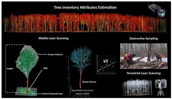
Graphical Abstract

1. Introduction

Forest inventories rely on a network of plots with a fixed radius and a systematic (or random) sampling scheme, covering a domain representative of the forest, to be characterized. Inventory plots are generally surveyed over decades to better understand forest dynamics and the growing stock. However, maintaining these plots is costly, labor intensive, and their number is constantly reduced due to disturbances [1]. These constraints limit the spatial distribution and temporal resolution of field surveys, making them inadequate to support current requirements for accuracy, spatial details, and timely updates [2]. The most valuable attributes that measure reference data in the field are species, diameter at breast height (DBH), and height. Allometric models are then used, based on these measurements, to predict individual tree volume or biomass. Predictions from individual tree models are typically aggregated at the plot level and used to either calibrate or train remote sensing-based models, as well as produce large area estimates [3]. In monocultures of well-studied species, allometric estimates can perform well [4]. However, they are less reliable in mixed forest stands or hardwood stands, with different tree ages where tree-to-tree variability is much greater [5]. The problem is that all trees with the same value of independent variables have the same model prediction for volume when, in reality, they can have very different volumes [3]. In these cases, using allometric equations may lead to uncertainties and cause bias that can propagate when scaling up to the stand level [6]. New methods are currently needed to set up and efficiently survey more plots that will serve as reference data for larger scale remote sensing tools and allometric relationship calibration.
Over the past decades, terrestrial laser scanning (TLS) has evolved from an experimental tool to a practical instrument for the accurate measurement of forest attributes [7]. This technology provides highly accurate data on 3D structures of forest scenes. It also allows non-destructive estimation of tree attributes, which would be otherwise impractical to measure in the field, e.g., stem curves, crown dimensions, wood volume, or above ground biomass (AGB) [8]. A significant breakthrough is the development of algorithms that can reconstruct realistic 3D models of trees from TLS point clouds. These models are referred to as quantitative structural models (QSM). QSM algorithms, such as TreeQSM [9] or SimpleTree [10], allow the estimation of woody volumes of standing trees. A review by [11], comparing estimates of tree volume and AGB from QSM against destructive measurement, have shown that QSMs are capable of estimating tree AGB with less than 10% bias [12]. Despite these significant advances to support field measurements, TLS has not yet been widely adopted by practitioners. The main limit is that TLS data acquisition requires time that exceeds what can be deemed reasonable for a field inventory. For example, covering a 400 m2 forest plot with a TLS may require from three to five scans, from different positions, to avoid occlusion, and it must include geo-referencing procedures to co-register the scans. These procedures require an average of 45 to 80 min of acquisition time for a single 400 m2 plot and generally need a support team. Considering that data pre-processing requires about the same amount of time, this entire process is beyond reasonable time frames for routine forestry applications. It remains to be demonstrated whether in-situ 3D scanning technologies can be used efficiently to the point of being adopted in operational forestry, in which tree and plot-level attributes can be recovered quickly, accurately, and at low cost [13].
Recently, mobile laser scanning (MLS) has demonstrated its potential for the effective assessment of tree and plot-level attributes [14]. MLS has several advantages over TLS [15,16]: increased speed for data acquisition (~3–10 min for scanning a 400 m2 sample plot); easier mobility between trees to avoid occlusion; reduced weight of the equipment; efficient data geo-location; affordability. Typical platforms used for MLS in forestry are generally equipped with a Global Navigation Satellite System (GNSS) receiver and an inertial measurement unit (IMU) for positioning and orientation [17]. Although these systems are very convenient in open areas, they are not useful under dense forest cover, due to poor GNSS reception. To overcome this limitation, new types of MLS systems that do not rely on a GNSS receiver have recently emerged. They use simultaneous localization and mapping (SLAM) algorithms to determine their position and orientation, with respect to their surroundings, while simultaneously mapping the environment. Several studies demonstrated that these devices offer centimeter-level accuracy [18,19].
The use of SLAM-based MLS in forestry is still at an early stage of development, but it may well meet the expectations of practitioners. Several studies have demonstrated their potential and accuracy for tree location and stem DBH retrieval [17,20]. Compared to TLS data, SLAM-based MLS point clouds are generally noisier or fuzzier [21], and they also have lower spatial accuracy due to propagation of positioning errors [22]. A recent study found that SLAM-based MLS systems estimated DBH with an average RMSE of about 1.8 cm [17]. Until recently, the most limiting factor of MLS sensors was their range [23]. However, new generations of SLAM-based MLS that have recently emerged on the market now provide a range of up to 100 m. This has allowed researchers to evaluate their potential to retrieve tree height and crown dimensions [24,25], showing great potential for supporting the development of allometric models. The quality of more complex tree attributes derived from contemporary MLS, such as stem taper or merchantable wood volume, remains unclear and is currently under investigation [22,26,27,28]. This study aimed to evaluate the potential of SLAM-based MLS data to estimate tree structural attributes in a temperate hardwood stand, including tree height, crown dimensions, DBH, and merchantable wood volume. Destructive field measurements and TLS data were used as reference to quantify errors on inventory attribute estimations from MLS data. The results of this paper are expected to provide a better understanding of the potential of SLAM-based MLS systems to support in-situ forest inventory.

2. Materials

2.1. Study Site

A 1 ha mature hardwood site was studied in Jardine Brook, southwest of Saint-Quentin (NB, Canada), at 280 m above sea level (47°25′21.70″N, 67°31′5.84″W) (Figure 1A). The study site belongs to the Central Uplands Ecoregion of Madawaska located in the temperate hardwood zone [29]. This region is characterized by a cold temperate climate with short, cool summers and long, cold winters, with average temperatures of 3.5 °C and precipitation of 1025 mm per year. The soil is of the Caribou type on ablation glacial till, with high fertility, medium texture, and deep depth to the water table (>9 m in the study area) [30]. The study site is located on flat terrain (slope < 1%), it has a crown closure of 56%, and it has little understory or shrub presence (Figure 1B). The trees from the 1 ha hardwood stand have an average height of 18 m (standard deviation of 5.6 m) and an average crown base height of 7.6 m (standard deviation of 2.9 m). The stand has not received high intensity treatments, except for very light removals (<10% basal area) to salvage balsam fir mortality, since the early 1940s. The stand contains about 500 merchantable stems per hectare (DBH ≥ 9 cm), has a basal area of 16 m2/ha, and is considered multi-age, having more than two distinct cohorts or age classes (from 75 to 160-years-old). The stand is mainly composed of sugar maple (Acer saccharum Marshall) (88% basal area), yellow birch (Betula alleghaniensis Britton, 10%), and balsam fir (Abies balsamea (L.) Miller, 2%).

2.2. Field Measurements

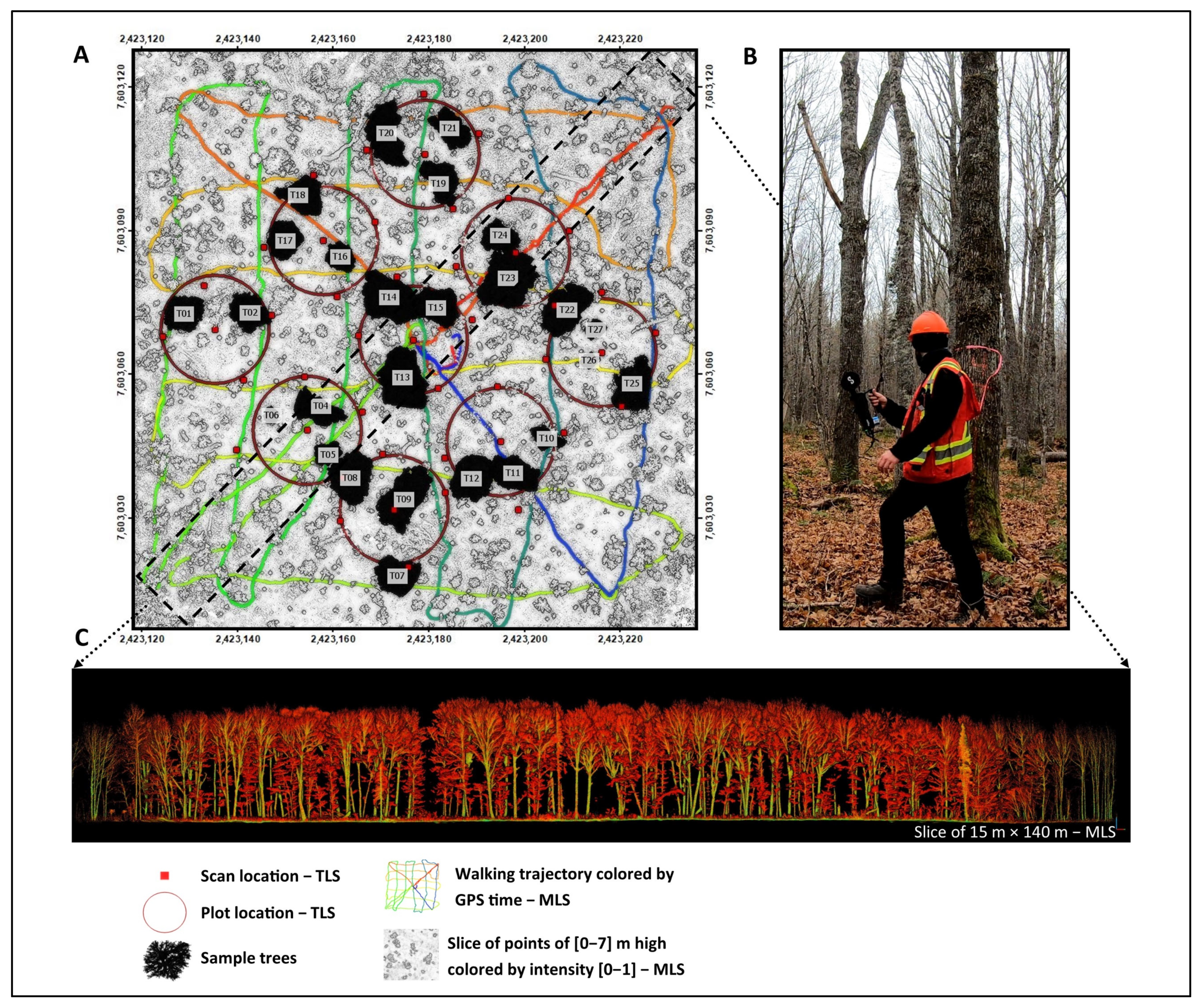
Field measurements were collected in October 2021. Nine sample plots of 11.28 m radius (400 m2) were established within the 1 ha study site (Figure 2A). A total of 26 sample trees (about 3 trees per plot) were selected to be destructively sampled immediately after cutting and bucking by a single-tree harvester. DBH (at 1.3 m) was measured with a measuring tape. The mean and standard deviation of DBH, for the 26 sample trees in our study site, were 41.8 cm and 10.4 cm, respectively. These trees were numbered and tagged with a retro-reflective checkboard to enable their quick identification in the TLS and MLS data and for easy linking to the inventory data. They were geo-referenced using FC-500 Hiper SR Kit Rover (TopCon Positioning Systems Inc., Livermore, CA, USA).
The 26 sample trees were felled and bucked into segments in March 2022. The harvester placed each segment to be measured in two distinct areas: one with all stem segments coming from below the crown base height (i.e., where branches spited the main stem) and a second with all the branches with the smallest piece being longer than 244 cm and with a small end diameter outside bark (DOB) of greater than 8 cm. Post-harvest measurement on each felled trees included: (i) stump height, (ii) length of each segment, and (iii) widest and narrowest DOB at the end of each segment. These measurements were used to calculate the operational merchantable volume per tree (see merchantable wood volume nomenclature, defined in Section 3.3, and the accuracy assessment in Section 3.4).

2.3. Terrestrial Laser Scanning (TLS) Data

The TLS data were acquired in leaf-off conditions, in October 2021, using a FARO Focus3D S 120 (Faro Technologies Inc., Lake Mary, FL, USA). The nine inventory sample plots, similar to those used for field measurements, were scanned to obtain point clouds of the 26 sample trees. The scans were done from five location (i.e., the plot center and the four cardinal points of the plot) to minimize laser signal occlusion (Figure 2A). The center-point of each TLS plot was measured with the TopCon FC-500 Hiper SR Kit Rover (Topcon Positioning Systems, Inc., Livermore, CA, USA). The location of the 26 trees, as well as these center-point locations, were used as references to geo-reference the TLS point cloud and to co-register the scans with the MLS data. The scanner was parameterized to obtain a point spacing of 6.3 mm at 10 m distance from the sensor (i.e., quality: 3×; resolution: ¼). Eight spherical targets were spread within the sample plots to allow scan co-registration within the FARO SCENE 5.1.6.3 software (FARO, Lake Mary, FL, USA). The scan co-registration process reported a mean absolute error of 6.0 mm.

2.4. Mobile Laser Scanning (MLS) Data

The MLS data were acquired in leaf-off conditions in October 2021 using a handheld Emesent Hovermap (Emesent Pty Ltd., Milton, QLD, Australia) (Figure 2B). The Hovermap includes a Velodyne VLP-16 Lite lidar (Velodyne Lidar Inc., Morgan Hill, CA, USA), a data logger (1.8 kg), and an inertial measurement unit (IMU). The VLP-16 has 16 lidar channels and measures up to 600,000 points per second, in dual return mode, within a maximum range of 100 m. The distances are recorded with a continuous wavelength of 903 nm and with a lidar accuracy of ±3 cm. The Hovermap uses SLAM technology, allowing it to create a 3D point cloud without the use of artificial reference targets or tripods. It uses the lidar and IMU data for an instantaneous location of the sensor and generates a coherent map of its surroundings. However, loop closure (i.e., using the same point for start and finish) is highly recommended to update real-time mapping and adjust the MLS trajectory.
Data acquisition with the Hovermap was performed by walking within the study site while the rotating scanner captured lidar data. The 1 ha study site was scanned in a 45-min walk following a 20 m × 20 m grid pattern (Figure 2A). At each corner of the study site, we circled back to the stand center to close the loop several times and adding several viewing perspectives. This design was selected to optimize coverage of the sample plots and to perform a loop closure trajectory for reducing potential drifts associated with the SLAM algorithm. Hovermap data (Figure 2C) were automatically preprocessed in 3 h using the proprietary software Emesent 1.5.0 (Milton, Australia).

3. Methods

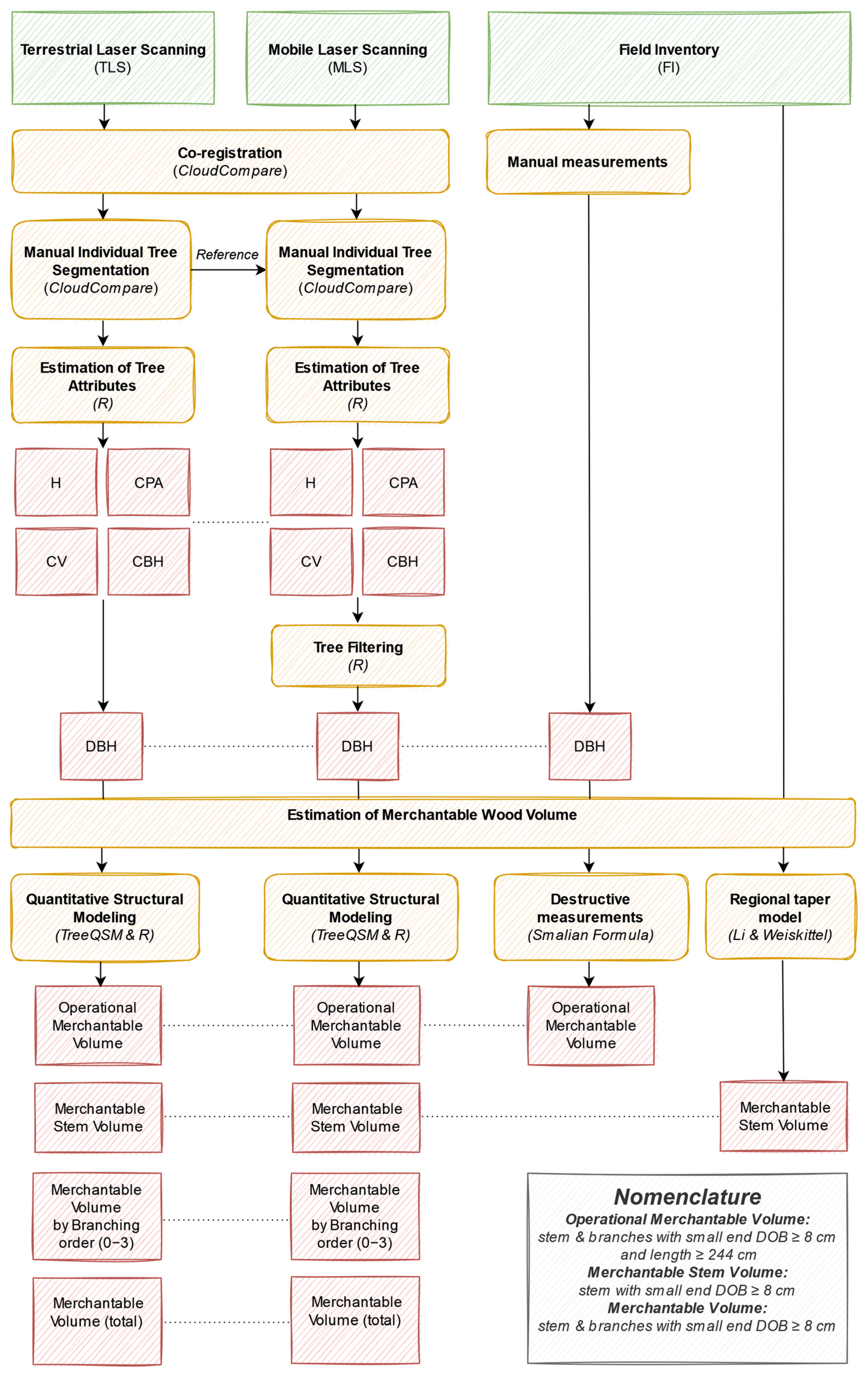
The overall data processing workflow for TLS and MLS, in Figure 3, shows the main steps performed in this study to extract tree structural attributes. These steps included: (i) co-registration and manual individual tree segmentation of TLS and MLS data (Section 3.1); (ii) estimation of tree attributes (Section 3.2); (iii) tree filtering (Appendix A); (iv) estimation of merchantable wood volume (Section 3.3). The three types of merchantable wood volume estimated in this workflow were defined as follows:
  • Operational merchantable volume: volume of the stem and all branches of a tree, with the smallest segment being longer than 244 cm with a small end DOB ≥ 8 cm;
  • Merchantable stem volume: volume of the stem, with a small end DOB ≥ 8 cm (i.e., the main stem to the top of a tree excluding branches);
  • Merchantable volume: volume of the stem and all branches of a tree with a small end DOB ≥ 8 cm.
For the accuracy assessment on estimated attributes (Section 3.4), field measurements were used as reference for DBH and operational merchantable volume. The reference taper model used in the Acadian region (Section 3.4) was compared to the merchantable stem volume derived by the lidar QSMs to provide valuable guidance to foresters. When attributes estimated by the field measurements were either inaccurate or unavailable (such as tree height (H), crown projected area (CPA), crown volume (CV), crown base height (CBH), and merchantable volume per branching order), the attributes estimated from MLS data were compared to the one estimated from TLS data.

3.1. Manual Individual Tree Segmentation

The application of automatic tree segmentation algorithms can impact the estimation of tree structural attributes [31]. Therefore, in this study, we adopted manual segmentation of the sample trees based on visual separability. This was done to minimize the impact of the segmentation process in assessing the accuracy of the estimated tree attributes. To do this, the nine geo-referenced TLS sample plots were first co-registered with the MLS point cloud using CloudCompare’s fine registration Iterative Closest Point (ICP) algorithm [32]. Each sample tree was then located in the TLS and MLS point cloud using the base and rover data, as well as its retro-reflective checkboard. The 26 sample trees were manually segmented from TLS and MLS point clouds using the “segment” tool from CloudCompare. The TLS sample trees were used as reference to assist the MLS manual tree segmentation. The average root-mean-square (RMS) error that was calculated automatically by the co-registration algorithm, over 50,000 points of the 26 TLS and MLS segmented trees pairs, was 3.6 cm. The TLS and MLS point clouds of the 26 manually segmented trees are presented in Figure 4.

3.2. Estimation of Tree Attributes

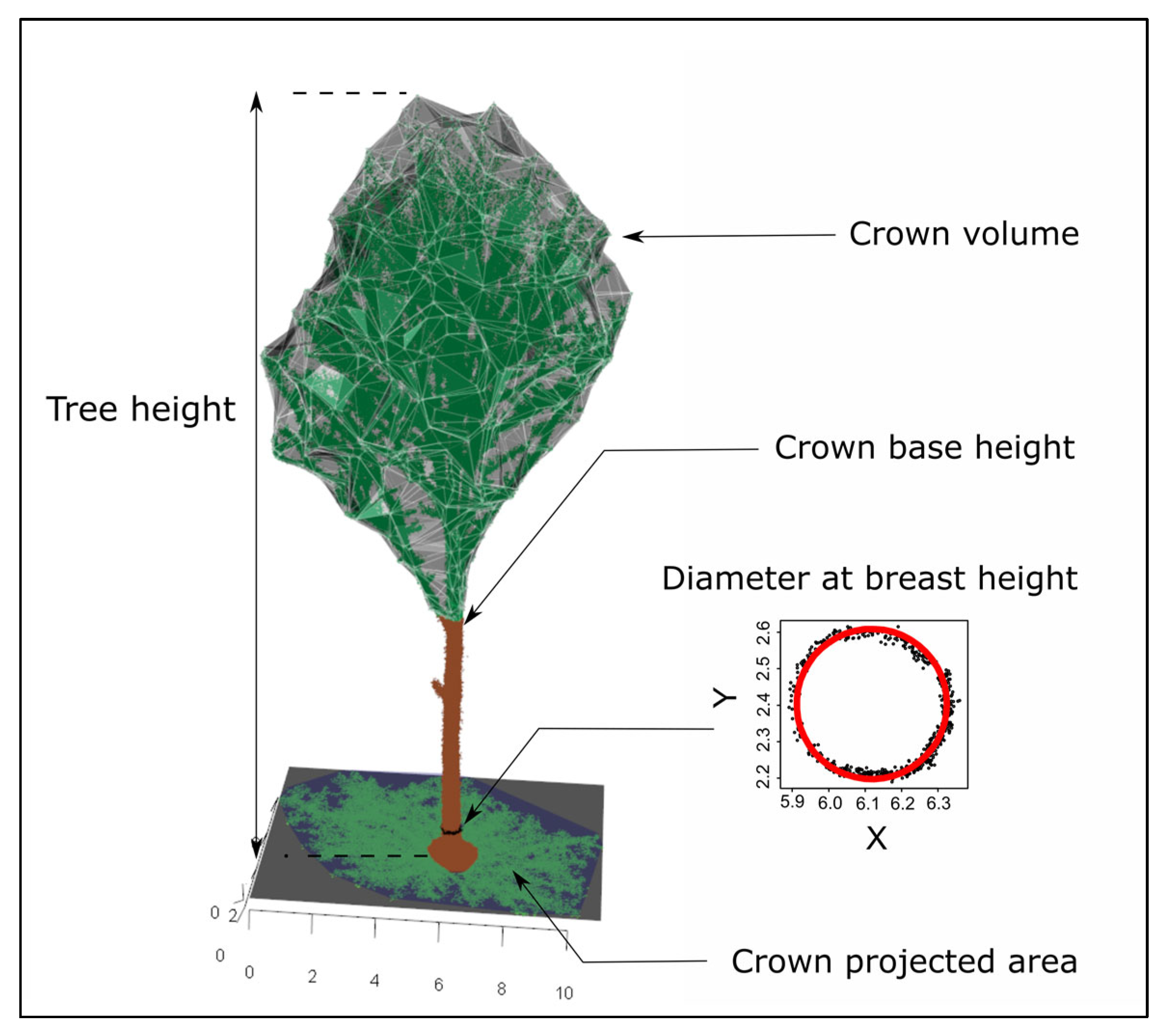
Tree H, CBH, CPA, CV, and DBH were estimated from the TLS and MLS point clouds of all manually segmented trees (Figure 5). All of these attributes were computed using R [33]:
  • H was estimated as the difference between the highest and the lowest point of the manually segmented tree point cloud;
  • CBH was determined using the approach that was described in [34] and used in [31];
  • CPA was determined using the area of the convex hull that was computed on the crown points projected in the xy-plane. The crown points are defined as the points higher than the identified CBH;
  • CV was determined using an alpha shape computed on crown points (α = 1);
  • DBH was estimated by fitting a circle on the XY coordinates of a 5-cm wide point cloud slice, located between 1.275 and 1.325 m height above ground, using the R package “conicfit” [35]. The ground was considered as the lowest Z coordinates of the manually segmented tree point cloud.

3.3. Estimation of Merchantable Wood Volume

The point cloud of the MLS device is noisier than that of the TLS data. Therefore, attributes estimated from MLS data are less reliable. Noise intrinsic to the MLS data can, however, be limited by filtering the point cloud using two different approaches: (i) by using statistical outlier removal (SOR), which removes points that are farther than an average distance of a group of points; (ii) by using a range filter, which removes the points that were sampled farther than a threshold distance from the scanner. A SOR filter (k = 5, sigma = 1.5) was applied to the segmented point clouds using the R package “VoxR” (Version 1.0.0, available online at: https://CRAN.R-project.org/package=VoxR, accessed on 20 April 2022) [36]. Range filters of 15 m and 30 m were applied to the stem and the crown of each point cloud, respectively (see Appendix A for more detail on a sensitivity analysis on the filtering options).
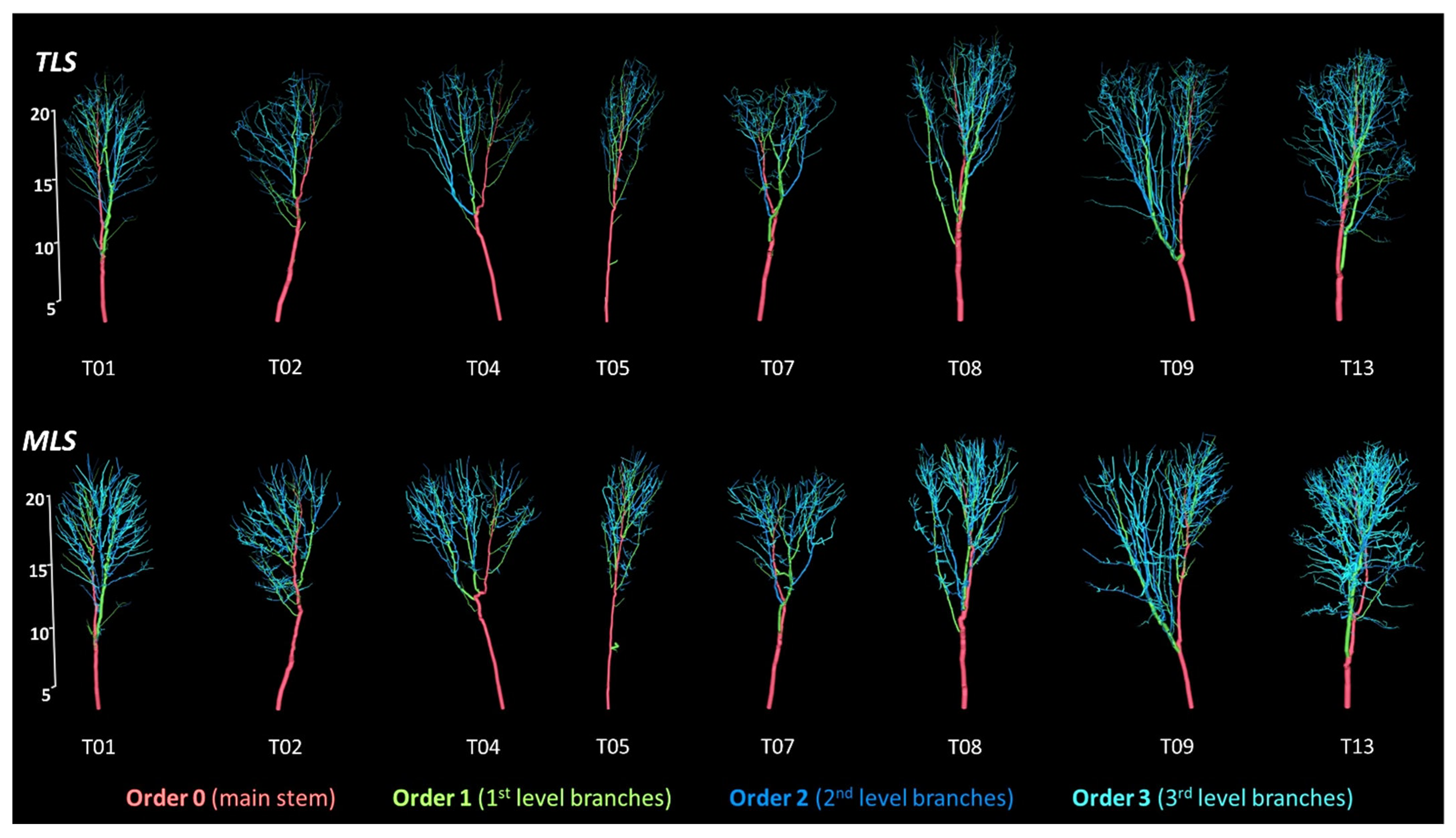
The QSM were generated for each tree using TreeQSM algorithm [9] (Figure 6). The approach described in [37] was used to optimize model parameters and select the best reconstruction. Comparison between the operational merchantable volume obtained from the destructive field measurements and that generated from QSMs were possible because all segments of the QSM smaller than 8 cm diameter were truncated, and the last branches that were shorter than 244 cm were removed using the R package “aRchi” [38]. The resulting modeled trees were, thus, consistent with the field protocol presented in Section 2.2. Additionally, the stem base of each TLS and MLS segmented tree was truncated at the stump height measured in the field after felling to match the destructive field reference. The QSMs included axes of four orders: order 0—main stem and 1st, 2nd, and 3rd-order branches (Figure 6). A fine analysis comparing merchantable volume of TLS and MLS by branching order (up to 3rd) was performed. Finally, the merchantable stem volume, extracted from lidar QSMs, was compared to the merchantable stem volume estimated with species–specific regional taper models developed by Li and Weiskittel [39,40] (Section 3.4).

3.4. Accuracy Assessment on Estimated Attributes

The reference operational merchantable volume was obtained by summing up the volume of each stem and branch segments measured in the field (Section 2.2) using the Smalian formula [41]. The length of each segment and the diameter from each segment’s end (calculated as the mean of the widest and narrowest DOB) were used as input parameters. The merchantable stem volume for each tree was calculated using the Li and Weiskittel taper model developed for hardwood species in the Acadian region [39,40]. Field DBH, TLS-derived tree heights, and species-specific parameters were used as inputs for the taper equations. The reference merchantable volume (by branching order and total) was computed from TLS QSMs (Section 3.3).
Accuracy of the estimated tree attributes (i.e., tree height, crown dimensions, DBH, and merchantable wood volumes) was assessed by calculating the coefficient of determination (R2) (Equation (1)), root-mean-square error (RMSE) (Equation (2)), and bias (Equation (3)):
R 2 = 1 i = 1 n ŷ i y i 2 i = 1 n ȳ i y i 2 ,
RMSE = 1 n   i = 1 n ( ŷ i y i ) 2 ,
bias = 1 n   i = 1 n ( ŷ i y i ) ,
where n represents the number of trees, y i is the reference field inventory/TLS attribute that was measured for t r e e i , ŷ i is the estimated attribute for t r e e I , and ȳ i is the mean of the field inventory/TLS reference attribute.

4. Results

4.1. Tree Height, Crown Dimensions and DBH

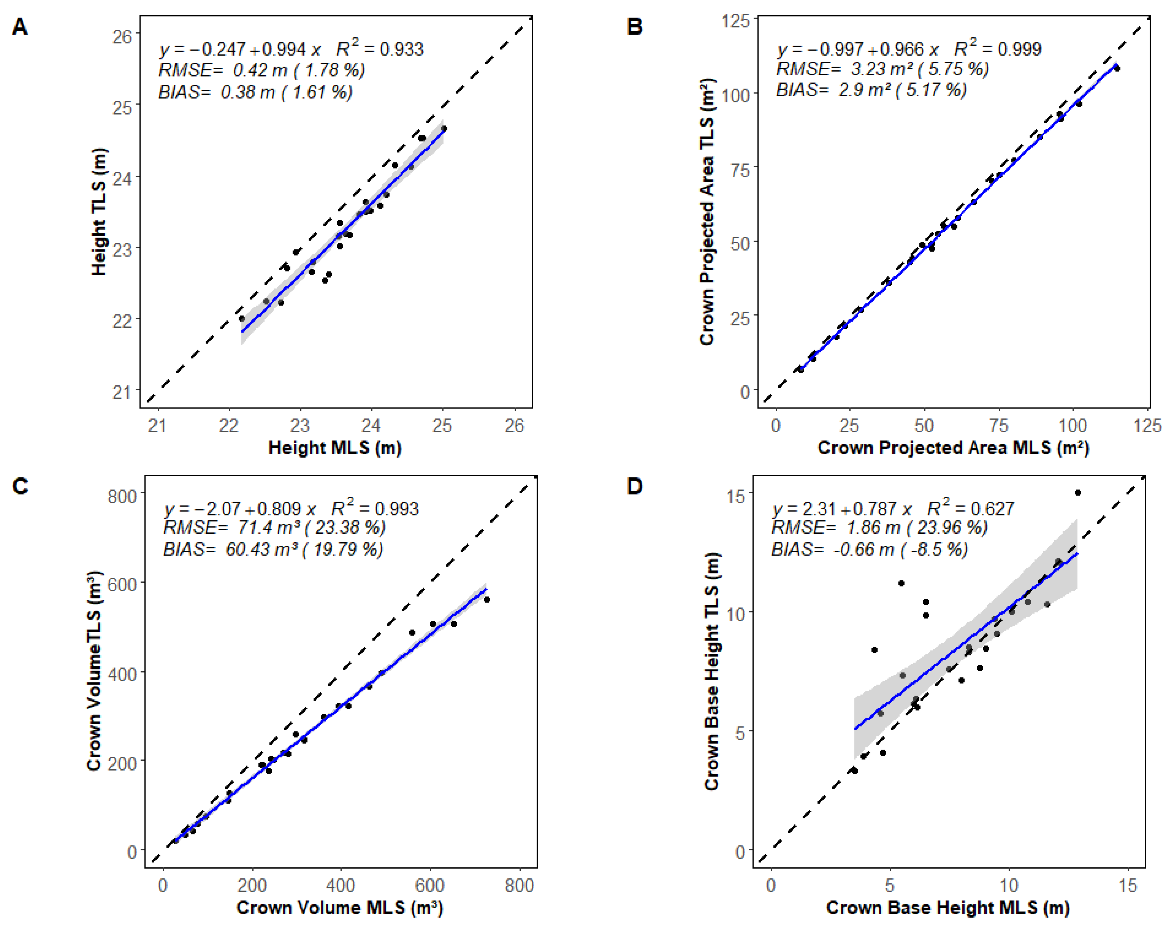
Crown attributes derived from TLS and MLS data show great similarity. The tree height and CPA estimates from the MLS data show a good agreement with TLS data, with an RMSE of 0.42 m (1.78%) (Figure 7A) and 3.23 m2 (5.75%) (Figure 7B), respectively. The MLS crown volume is overestimated, with an RMSE of 71.4 m3 (23.38%), which tends to increase for larger crowns when compared to those estimated from TLS data (Figure 7C). This overestimation is related to the underestimation of the crown base height that was observed for the MLS trees, which increases crown volume (Figure 7D).
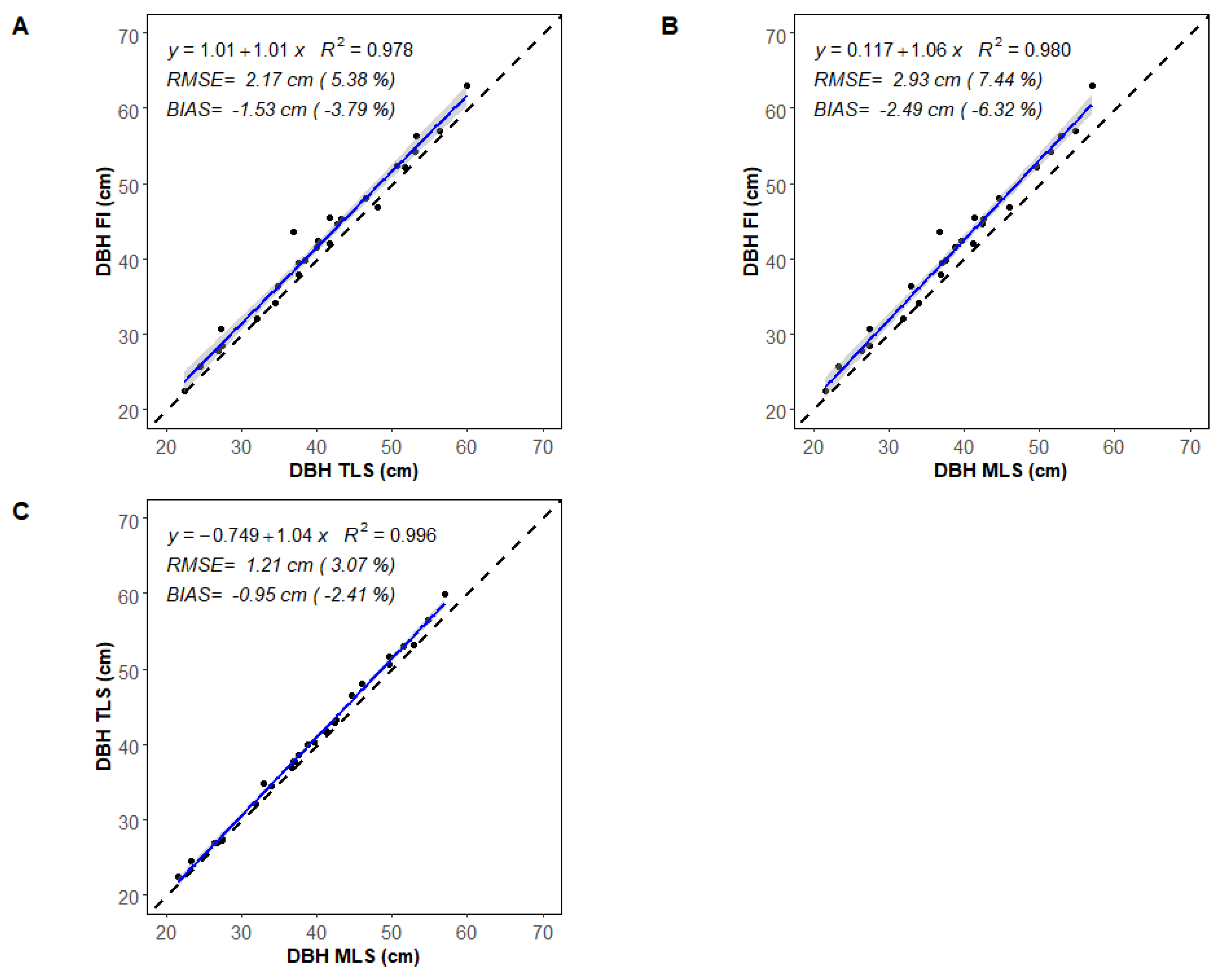
In comparison to field measurements, TLS and MLS data show similar reliable DBH estimates, with a negative bias of 1.53 cm and 2.49 cm, respectively (Figure 8A,B). The strong relationship between DBH, estimated by TLS and MLS data (R2 = 0.99; RMSE = 1.21 cm (3.07%), Figure 8C), shows that, despite MLS data being noisier, the circle-fitting method gave very similar results for TLS and MLS point clouds.

4.2. Merchantable Wood Volume (QSM)

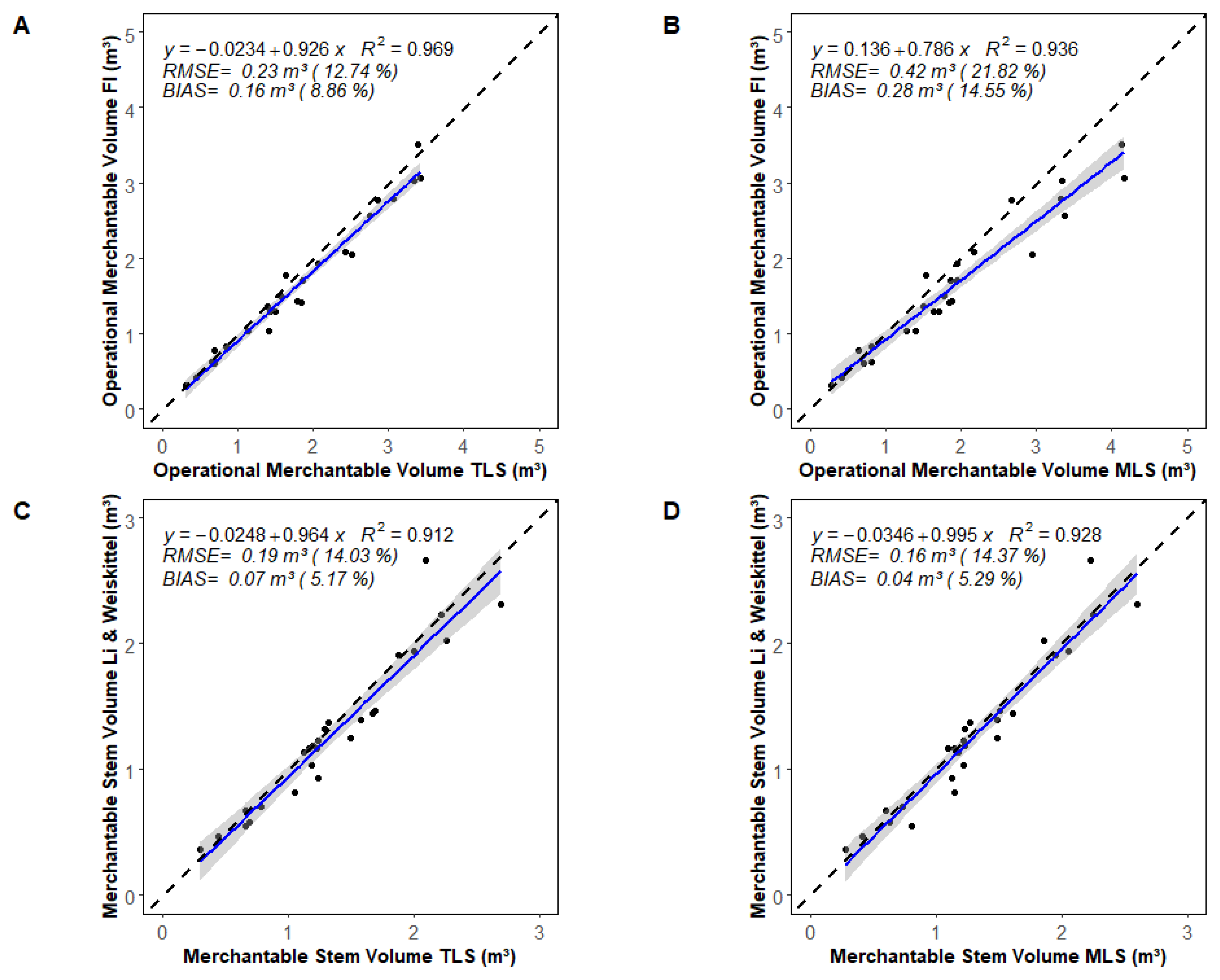
The operational merchantable volume (i.e., stem and branches with small end DOB ≥ 8 cm and length ≥ 244 cm) was overestimated by both TLS (RMSE = 0.23 m3 or 12.7%) and MLS (RMSE = 0.42 m3 or 21.8%) QSMs (i.e., branching order 0–3 with small end DOB ≥ 8 cm and length ≥ 244 cm) when compared with destructive measurements (Figure 9A,B). The deviation with the 1:1 line shows that this overestimation increases with the tree dimensions, especially for the MLS data.
The merchantable stem volume, estimated with the QSMs (i.e., branching order 0 with small end DOB ≥ 8 cm), is strongly related to the merchantable stem volume derived from Li and Weiskittel’s taper model (Figure 9C,D). Estimates from the taper model match those from TLS QSMs (Figure 9C) and MLS QSMs (Figure 9D), with R2 = 0.91 and 0.93, as well as a bias of 0.07 and 0.04 m3, respectively.
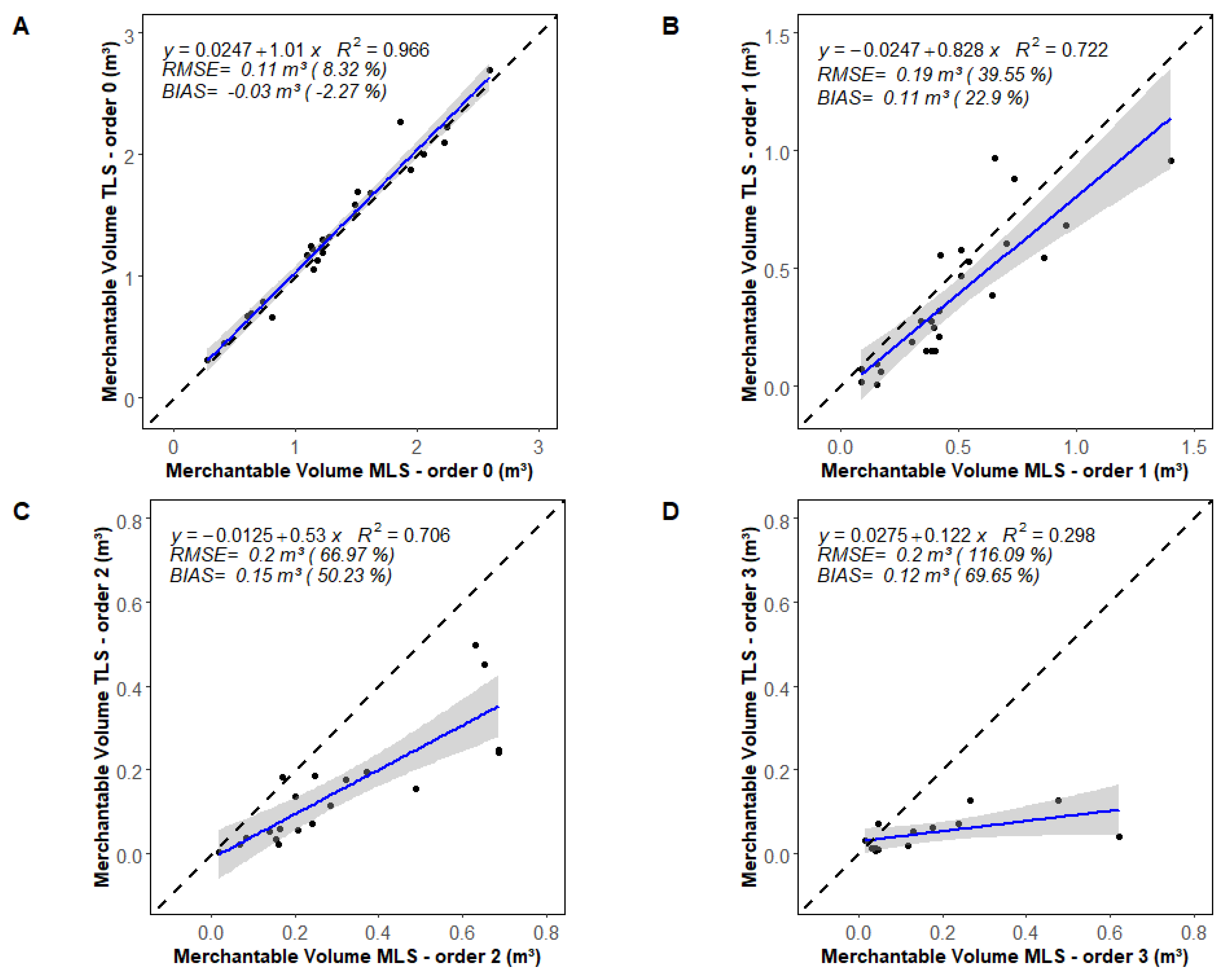
The merchantable volume, estimated by TLS and MLS QSMs presented by branching order (Figure 10), showed that the merchantable stem volume estimated by TLS and MLS QSMs (i.e., branching order 0 with small end DOB ≥ 8 cm) is very similar (R2 = 0.96, RMSE = 0.11 m3 (8.3%) (Figure 10A). However, the branching volume (i.e., order 1 = first branches, order 2 = second branches, and order 3 = third branches; with small end DOB ≥ 8 cm) is systematically overestimated by the MLS QSMs (Figure 10B–D). This overestimation increases substantially with increasing branching order.
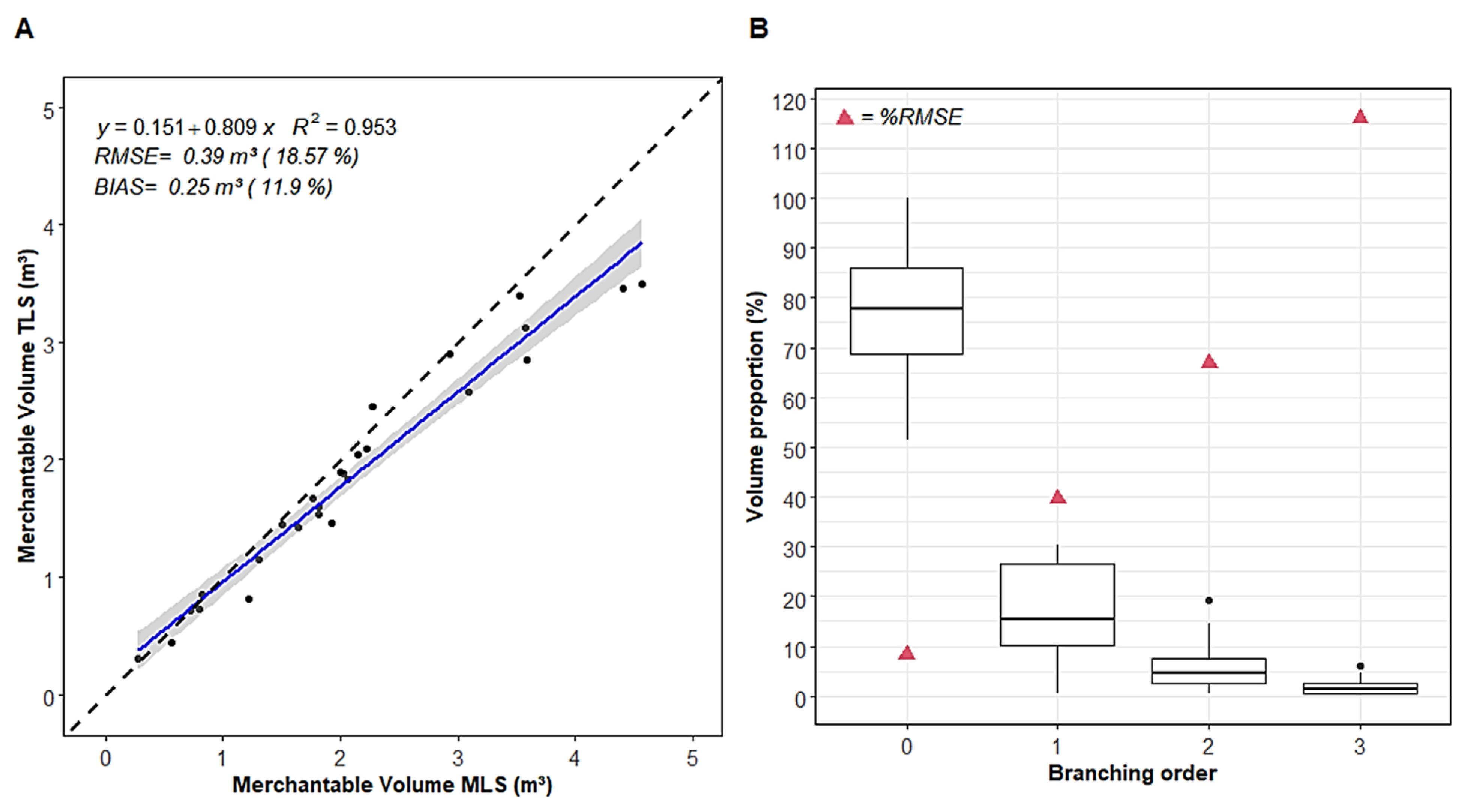
Merchantable volumes that were estimated by TLS and MLS QSMs (order 0–3 with small end DOB ≥ 8 cm) are very similar but show some overestimation of total volume from MLS data (R2 = 0.95, RMSE = 0.39 m3 (18.6%); Figure 11A). The proportion of merchantable volume for each branching order is illustrated in Figure 11B. Boxplots show that the biggest proportion of merchantable volume belongs to the main stem (order 0; mean = 78%) and the first level of branches (order 1; mean = 17%). However, the second and third levels of branches represent, on average, only 6% and 2% of the total merchantable volume, respectively. Therefore, the significant increase in %RMSE (red triangles) observed for second and third-order branching does not have a major effect on estimated total merchantable volume.

5. Discussion

The study compared tree attribute estimates from field measurements, TLS, and MLS data. To the best of our knowledge, no other study has evaluated the potential of SLAM-based MLS data for extracting merchantable wood volume of hardwood trees using a QSM approach. Overall, the estimates from MLS data provided good results. Our work suggests that, with the use of adapted filters to attenuate noise, the estimates of crown and stem attributes are very close to those from TLS data. Although the estimation from MLS data performed well for the volume of the main stem, branching volume tends to be overestimated with gradual bias with branching order. However, the effect of these errors is limited because 2nd and 3rd-order branching only represented a small proportion of total wood volume. In the following sections, we compare the accuracy of each estimated attributes with past studies and highlight some applicability and further development of SLAM-based MLS systems for supporting in-situ forest inventory.

5.1. Comparison of Estimated Attributes with Past Studies

Diameter at Breast Height—DBH was estimated with high accuracy from both TLS and MLS data (Figure 8) with no major difference observed between the two laser systems (Figure 8C). Comparable results of DBH estimates were obtained in [42] with an RMSE of 2.32 cm (12.01%) with MLS data and 2.55 cm (13.19%) with TLS data, when compared with field measurements. Similarly, ref. [43] used a SLAM-based MLS system and achieved a high accuracy with an RMSE of 2.45–2.93 cm (4.7%–5.8%). Conversely, more accurate estimates of DBH were achieved in a boreal coniferous forest by [44], with an RMSE of 1.5 cm (7.5%) between the estimates from field measurements and MLS data. The lower accuracy of DBH, observed in this study when compared to field measurements (Figure 8A,B), may be explained by the non-circular shape of some of the hardwood sample trees. Surprisingly, both TLS and MLS data underestimated DBH values. The main reason for this underestimation lies in the circle-fitting method that fits a circle to the center of the point slice (Figure 5), introducing a negative bias compared to the field measurements. The use of spline-based models may improve DBH accuracy, but they require more careful adjustment of the parameters, based on the point cloud quality, compared to circle fitting algorithms [45].
Tree Height—Several previous studies have highlighted the low accuracy of estimates from MLS data for tree height because of the limited range of the sensor [18,46]. For example, ref. [18] compared the accuracy of the SLAM-based MLS ZEB-REVO (GeoSLAM Ltd., Nottingham, UK) with TLS data in two test sites and observed an RMSE of 1.3 m and 9.4 m, while [46] observed a bias of −4.61 m and an RMSE of 2.15 m with the ZEB1 (GeoSLAM Ltd., Nottingham, UK). Compared to these previous studies, the Hovermap system we used displayed low uncertainties for tree height measurements (Figure 7A). Similar observations were made by the recent studies of [47,48] that both used the ZEB-Horizon (GeoSLAM Ltd., Nottingham, UK), which has a range of 100 m. In [47], tree heights were estimated with an RMSE of 1.11 m and a positive bias of 0.45 m, compared to field-measured heights. In [48], tree heights were estimated with an RMSE of 1.8 m (8.7%) and bias of 1.3 m (6%) in open stands, as well as an RMSE of 1.1 m (4.9%) and bias of 0.68 m (3%) in denser stands, when compared with the ALS data used as reference. Both studies slightly overestimated tree height using recent MLS systems, which is in agreement with our results. It is likely that some treetops are captured more accurately by MLS point clouds than by TLS since TLS is a static system, which is more prone to occlusion than MLS. Overall, we find that, in our leaf-off temperate hardwood forest case (Figure 2C), where sample trees were 22–25 m tall, the Hovermap SLAM-based MLS system was able to estimate tree heights with high accuracy.
Crown Dimensions—The excellent relationship with TLS data (Figure 7B) demonstrated that MLS data captured the whole crowns and was reliable for extracting CPA. Due to the limited range of previous versions of SLAM-based MLS systems, only a few studies investigated their potential for hardwood crown dimension characterization. In [49], researchers used a vehicle-based Riegl VMX-250 MLS to estimate CPA with an RMSE of 2.2–2.9 m2 when compared to those estimated from TLS data, which is comparable to the results obtained in the current study. Using the same vehicle-based MLS system, [27] compared the CPA of 143 hardwood trees with TLS data and reported a mean difference of 5.61 m2. The slightly higher results observed in this study can be explained by the fact that we applied a manual TLS-assisted MLS trees segmentation, compared to [27], who used an automatic ITD algorithm. The overestimation of crown volume observed in Figure 7C is mainly related to a lower height that was identified by the CBH algorithm in MLS data (Figure 7D).
Merchantable Wood Volume—The potential of MLS data for merchantable wood volume estimation was evaluated at the stem and branch levels. At the stem level, the MLS showed small deviations from TLS estimates (Figure 10A) and from the Li and Weiskittel taper model (Figure 9D). At the branch level, wood volume from MLS data was systematically overestimated for fine branches (order 2 and 3; Figure 10C,D). This tendency to overestimate branching volume was also observed by [50] when using TLS data. This result was expected as distance from the scanner increased, resulting in a decreasing point-cloud quality and an increasing point spacing [48,51]. Moreover, topological errors in the QSM reconstructions can also result in volumetric inaccuracies [52]. Indeed, finer branch details are affected by the differences in topologies between TLS and MLS. These discrepancies in the two reconstructed structure models are observed in Figure 7 for trees T08 and T13. The slope recorded in Figure 10B–D suggests that a correction factor could, potentially, be introduced to compensate for this overestimation. Our results can be compared to those from [49], who used a vehicle-based Riegl VMX-250 MLS system to capture corridor-like 3D point clouds. They estimated merchantable volume for 24 hardwood trees using QSM, and they compared the accuracy of estimates from TLS and MLS data. They reported an RMSE of 0.4–0.6 m3 for merchantable volume, which is comparable to the results observed in this study (Figure 11A). Unlike our study, the merchantable volume estimated from the vehicle-based MLS QSMs was underestimated when compared to TLS data [49]. This underestimation of [49] was mainly caused by occlusion due to corridor-mapping acquisition, which was not observed in this study because of the free-range walking configuration. Overall, merchantable stem volume estimates from the SLAM-based MLS data, such as those from our study site and from [48], are close to the accuracy that is required for operational field inventory, e.g., a relative RMSE of 10%.

5.2. Applicability and Further Development

MLS is an effective and practical tool, in terms of data acquisition, for forest inventory. Compared to TLS, MLS offers a simpler way for producing accurate 3D point clouds in less time. Data collection does not require setting up co-registration targets or planning a priori positions for multiple scans. Instead, MLS only requires walking through the forest with an active sensor to minimize occlusion. In this study, scanning 1 ha took about 45 min with an MLS. In comparison, scanning nine 400 m2 sample plots (~0.28 ha) took about 12 h using TLS. Short acquisition times of MLS allow flexibility in the face of changing weather conditions, considering that lidar data are sensitive to wind, which introduces noise [53]. Another important aspect of MLS is its logistical compatibility with operational forestry. With a weight of about 1.8 kg and a simple on-off button to collect data, this device is easy to bring into the field and does not require extensive training. In addition, the preprocessing of SLAM-based MLS data is quite straightforward with almost automatic data processing. It is important to note that the preprocessing time increases considerably with the size of the file, e.g., about 10 min for traditional 400 m2 plots compared to 3–4 h for a hectare. Nevertheless, MLS data acquisition and preprocessing time is much lower when compared to TLS.
The flexibility of MLS data acquisition opens new opportunities for collecting data on large sample plots. In this study, we demonstrated that tree structural attributes can be accurately estimated from SLAM-based MLS data acquired over a 1 ha hardwood site. Similar observations were made with the Hovermap by [19] on a 2-ha conifer genetic trial. Interestingly, both of our studies performed a long-time acquisition with distinct walking patterns, and neither observed instrumental drift or registration inaccuracies in the point cloud, unlike what was previously reported by [42] with the GeoSLAM Horizon. In both acquisitions, the selected walking paths (i.e., 20 m × 20 m grid in this study (Figure 2) and 5 m parallel lines spacing in [19]) regularly revisited area previously scanned to meet the SLAM algorithm’s specification of “closing the loop”. We therefore suggest respecting these recommendations when collecting large area datasets. However, since these observations were made under favorable conditions (i.e., flat terrain with little low vegetation), further study is needed to determine how the walking pattern, forest structure, and sample plot size influence the quality of MLS point clouds [42,43]. Overall, acquiring ground-based lidar data on large sample plots, as performed in this study, holds promise for supporting a wide range of forestry studies that currently lack field reference data or are limited by the size of inventory sample plots (e.g., phenotyping, crown competition, leaf-area index, individual tree crown delineation, etc.).
In less than a decade, there has been significant progress in the development of QSM algorithms. The use of QSMs is now one of the most adopted approaches for processing ground-based point clouds from forested areas [52]. We are currently witnessing a transition from measuring individual tree attributes to full tree reconstruction. The current challenge of QSM application is to improve approachability in the reconstruction process, as it currently requires a great deal of expertise to optimize input parameters [37,52]. We also see a growing number of published and freely available algorithms for manipulating or reconstructing QSMs, such as SimpleTree [10], TreeQSM [9], AdTree [54] or aRchi [38]. However, most of these only work at the tree-level and require tedious manual editing to segment trees from a point cloud, as performed in this study. Further development is still needed to provide fully automatic stand-level solutions to support operational forestry, which are not yet reliable, especially in more complex environment such as a tropical forest [37]. With the increasing availability of QSM algorithms and the democratization of MLS technology, we expect to see, in the near future, new automatic approaches capable of processing larger-scale point clouds. Meanwhile, important steps would be to identify the potential and limitation of SLAM-based MLS technology for tree reconstruction in a variety of forest structures and terrain conditions to generalize conclusions beyond our study.

6. Conclusions

Allometric models used to estimate wood volume generally suffer from uncertainties about data traceability and calibration. TLS currently provides an efficient non-destructive alternative to reconstructing trees from point clouds and estimating volume from QSMs. Yet, TLS use in forest environments is costly, time-consuming, and requires a high-level of expertise to the point where it is impractical in an operational inventory program. In this study, we demonstrated the potential of MLS technology as a promising alternative to collecting non-destructive merchantable wood volume measurements. For the first time, a 1 ha hardwood site was scanned with a SLAM-based MLS system that enabled the extraction of highly accurate 3D point clouds and QSM reconstruction of trees. MLS allows for minimizing signal occlusion, one of the main limitations of TLS systems for tree reconstruction. Although MLS point clouds are still noisier than those from TLS, applying adapted filters to identify structure boundaries led to results that were almost comparable to those from TLS data. Despite needing more work to optimize MLS data collection and clarify the occlusion effect and completeness of the data in more complex forests environments, MLS technology could become an important tool to increase the collection of reference data in the field and feed allometries that are currently calibrated only on a small number of trees.

Author Contributions

Conceptualization, B.V., R.A.F., G.P. and P.L.; methodology, B.V., O.M.-D. and R.A.F.; software, B.V. and O.M.-D.; validation, B.V. and G.P.; formal analysis, B.V. and O.M.-D.; investigation, B.V.; resources, R.A.F. and G.P.; data curation, B.V.; writing—original draft preparation, B.V.; writing—review and editing, B.V., O.M.-D., R.A.F., G.P. and P.L.; visualization, B.V. and O.M.-D.; supervision, R.A.F. and P.L.; project administration, R.A.F. and G.P.; funding acquisition, R.A.F. and G.P. All authors have read and agreed to the published version of the manuscript.

Funding

This research was funded by a grant from the NSERC Discovery program to R.A. Fournier (RGPIN-2020-05780), by private funds from the Northern Hardwoods Research Institute Inc. (NHRI), and by Mitacs «Acceleration funding grant ref. FR60300».

Data Availability Statement

The data presented in this study are available on reasonable request from the corresponding author. The data are not publicly available because they were generated on private land and are subject to a confidentiality agreement with the landowner.

Acknowledgments

We thank NHRI for providing the datasets used in this paper. We are particularly grateful to Pamela Hurley-Poitras for her extensive technical and logistical support throughout the study and for organizing and collecting the destructive measurements. We thank Jeff Smith for geo-referencing the data and assisting with data collection and GIS processing. We are also grateful to RMUS, our technical partners, for sharing their expertise on the use of the Hovermap MLS system. Special thanks to J.D. Irving Limited for allowing us to conduct this study in one of their hardwood stands and for felling and bucking the sampled trees. We thank Udayalakshmi Vepakomma from FPInnovations for her advice on data analysis and W.F.J. Parsons for the english revision.

Conflicts of Interest

The authors declare no conflict of interest. The funders had no role in the design of the study; in the collection, analyses, or interpretation of data; in the writing of the manuscript; or in the decision to publish the results.

Appendix A. Point Cloud Filtering Evaluation

MLS point clouds are noisier than those from TLS. As a result, attributes estimated from MLS may be less reliable, especially for QSM reconstructions, where small noise can lead to significant bias in the volume estimate. However, the noise intrinsic to the MLS data can be limited by filtering the point cloud using two different approaches: (i) statistical outlier removal (SOR), which removes points whose distance is greater than the average distance of a group of points plus a delta value. This filter results in a sharper contour of the stem and branching system point clouds, which in turn can lead to better QSMs reconstruction. And (ii), the range filter that removes points that were sampled at a distance greater than a threshold from the scanner. The further away from the scanner, the noisier the point cloud is due to SLAM co-registration uncertainties. A sensitivity analysis of these two filters was performed to select the best combination of filters to generate reliable QSMs.
Five trees were randomly selected from the 26 trees studied and their characteristics are summarized in Table A1. For each tree, eight filtering modalities were applied:
  • No filter
  • SOR filter only
  • Range filter at 15 m only
  • Range filter at 20 m only
  • Range filter at 30 m only
  • SOR + Range filter at 15 m
  • SOR + Range filter at 20 m
  • SOR + Range filter at 30 m
Note that the range filter was applied below the crown only (i.e., the stem) to avoid suppressing actual points in the crown that are higher than the range filter threshold. However, we decided to systematically apply a range filter of 30 m to the crown to limit noise. Considering that the tallest tree in the sample is 25 m, 30 m is reasonable.
For the SOR filter, the recommended default values were used: k = 5 and sigma = 1.5. k being the number of the closest point used to compute the mean distance and sigma being the multiplier of standard deviation to consider a point as noise when added to the mean distance value. The R package “VoxR” was used to applied SOR filtering [36].
Table A1. Tree metrics of the five randomly selected trees.
IDH (m)CBH (m)CPA (m2)CV (m3)DBH (cm)
T0423.38.549.221737.6
T0523.210.417.873.427.2
T1523.78.354.9244.437.7
T2223.2677.2366.659.9
T2324.712.2108.1505.156.6
For each filtering modality of each tree, a QSM was computed with the same approach used in the main manuscript and described in [37]. The merchantable wood volume of the main axis (order 0) and the first order branches (order 1) was computed and summed for each QSM and compared to the TLS values in order to estimate errors associated with each modality. Only order 0 and 1 were chosen for this analysis, as 95% of the volume in average is contained within these two orders (Figure 11) and strong uncertainties are associated with the reconstruction of higher branching orders, even for TLS based reconstructions. Two metrics were used to estimate the error: absolute errors (AE in m3) (Equation (A1)) and relative error (RE in %) (Equation (A2)):
A E = V o l M L S V o l T L S
R E = A E V o l T L S
With V o l M L S being the merchantable wood volume of order 0 and 1 extracted from the QSM based on the MLS point cloud and V o l T L S being the merchantable wood volume of order 0 and 1 extracted from the QSM based on the TLS point cloud of the same tree.
Results are illustrated in Figure A1. We observe that applying filters significantly reduces the volume estimation error, with a relative error reaching around 10% when no filters are applied. The SOR filter is efficient because it always allows a significant reduction in merchantable wood volume estimation errors (i.e., the four best filtering modalities all include a SOR filter). The SOR filter combined with a 15 m range filter of the stem offers the best combination by reducing the error to 2.7% on average. This latter combination was used to perform the global analysis on the 26 trees studied in the main manuscript.
Figure A1. Relative (%) and absolute (m3) merchantable wood volume error distribution of each filtering modality for five trees randomly chosen among the 26 trees.
Remotesensing 14 04522 g0a1

References

  1. Luoma, V.; Saarinen, N.; Wulder, M.A.; White, J.C.; Vastaranta, M.; Holopainen, M.; Hyyppä, J. Assessing Precision in Conventional Field Measurements of Individual Tree Attributes. Forests 2017, 8, 38. [Google Scholar] [CrossRef]
  2. Achim, A.; Moreau, G.; Coops, N.C.; Axelson, J.N.; Barrette, J.; Bédard, S.; Byrne, K.E.; Caspersen, J.; Dick, A.R.; D’Orangeville, L.; et al. The Changing Culture of Silviculture. For. Int. J. For. Res. 2021, 95, 143–152. [Google Scholar] [CrossRef]
  3. McRoberts, R.E.; Westfall, J.A. Effects of Uncertainty in Model Predictions of Individual Tree Volume on Large Area Volume Estimates. For. Sci. 2014, 60, 34–42. [Google Scholar] [CrossRef]
  4. Muukkonen, P. Generalized Allometric Volume and Biomass Equations for Some Tree Species in Europe. Eur. J. For. Res. 2007, 126, 157–166. [Google Scholar] [CrossRef]
  5. Forrester, D.I.; Pretzsch, H. Tamm Review: On the Strength of Evidence When Comparing Ecosystem Functions of Mixtures with Monocultures. For. Ecol. Manag. 2015, 356, 41–53. [Google Scholar] [CrossRef]
  6. Vorster, A.G.; Evangelista, P.H.; Stovall, A.E.L.; Ex, S. Variability and Uncertainty in Forest Biomass Estimates from the Tree to Landscape Scale: The Role of Allometric Equations. Carbon Balance Manag. 2020, 15, 8. [Google Scholar] [CrossRef]
  7. Calders, K.; Adams, J.; Armston, J.; Bartholomeus, H.; Bauwens, S.; Bentley, L.P.; Chave, J.; Danson, F.M.; Demol, M.; Disney, M.; et al. Terrestrial Laser Scanning in Forest Ecology: Expanding the Horizon. Remote Sens Environ. 2020, 251, 112102. [Google Scholar] [CrossRef]
  8. Wilkes, P.; Lau, A.; Disney, M.; Calders, K.; Burt, A.; Gonzalez de Tanago, J.; Bartholomeus, H.; Brede, B.; Herold, M. Data Acquisition Considerations for Terrestrial Laser Scanning of Forest Plots. Remote Sens Environ. 2017, 196, 140–153. [Google Scholar] [CrossRef]
  9. Raumonen, P.; Kaasalainen, M.; Markku, Å.; Kaasalainen, S.; Kaartinen, H.; Vastaranta, M.; Holopainen, M.; Disney, M.; Lewis, P. Fast Automatic Precision Tree Models from Terrestrial Laser Scanner Data. Remote Sens. 2013, 5, 491–520. [Google Scholar] [CrossRef]
  10. Hackenberg, J.; Spiecker, H.; Calders, K.; Disney, M.; Raumonen, P. SimpleTree—An Efficient Open Source Tool to Build Tree Models from TLS Clouds. Forests 2015, 6, 4245–4294. [Google Scholar] [CrossRef]
  11. Demol, M.; Wilkes, P.; Raumonen, P.; Krishna Moorthy, S.; Calders, K.; Gielen, B.; Verbeeck, H. Volumetric Overestimation of Small Branches in 3D Reconstructions of Fraxinus Excelsior. Silva. Fennica. 2022, 56, 1–26. [Google Scholar] [CrossRef]
  12. Burt, A.; Boni Vicari, M.; da Costa, A.C.L.; Coughlin, I.; Meir, P.; Rowland, L.; Disney, M. New Insights into Large Tropical Tree Mass and Structure from Direct Harvest and Terrestrial Lidar. R. Soc. Open Sci. 2021, 8, 201458. [Google Scholar] [CrossRef]
  13. Liang, X.; Hyyppä, J.; Kaartinen, H.; Lehtomäki, M.; Pyörälä, J.; Pfeifer, N.; Holopainen, M.; Brolly, G.; Francesco, P.; Hackenberg, J.; et al. International Benchmarking of Terrestrial Laser Scanning Approaches for Forest Inventories. ISPRS J. Photogramm. Remote Sens. 2018, 144, 137–179. [Google Scholar] [CrossRef]
  14. Liang, X.; Kukko, A.; Hyyppä, J.; Lehtomäki, M.; Pyörälä, J.; Yu, X.; Kaartinen, H.; Jaakkola, A.; Wang, Y. In-Situ Measurements from Mobile Platforms: An Emerging Approach to Address the Old Challenges Associated with Forest Inventories. ISPRS J. Photogramm. Remote Sens. 2018, 143, 97–107. [Google Scholar] [CrossRef]
  15. di Stefano, F.; Chiappini, S.; Gorreja, A.; Balestra, M.; Pierdicca, R. Mobile 3D Scan LiDAR: A Literature Review. Geomat. Nat. Hazards Risk 2021, 12, 2387–2429. [Google Scholar] [CrossRef]
  16. Liang, X.; Hyyppa, J.; Kukko, A.; Kaartinen, H.; Jaakkola, A.; Yu, X. The Use of a Mobile Laser Scanning System for Mapping Large Forest Plots. IEEE Geosci. Remote Sens. Lett. 2014, 11, 1504–1508. [Google Scholar] [CrossRef]
  17. Balenović, I.; Liang, X.; Jurjević, L.; Hyyppä, J.; Seletković, A.; Kukko, A. Hand-Held Personal Laser Scanning—Current Status and Perspectives for Forest Inventory Application. Croat. J. For. Eng. 2020, 42, 165–183. [Google Scholar] [CrossRef]
  18. Cabo, C.; del Pozo, S.; Rodríguez-Gonzálvez, P.; Ordóñez, C.; González-Aguilera, D. Comparing Terrestrial Laser Scanning (TLS) and Wearable Laser Scanning (WLS) for Individual Tree Modeling at Plot Level. Remote Sens. 2018, 10, 540. [Google Scholar] [CrossRef]
  19. Hartley, R.J.L.; Jayathunga, S.; Massam, P.D.; de Silva, D.; Estarija, H.J.; Davidson, S.J.; Wuraola, A.; Pearse, G.D. Assessing the Potential of Backpack-Mounted Mobile Laser Scanning Systems for Tree Phenotyping. Remote Sens. 2022, 14, 3344. [Google Scholar] [CrossRef]
  20. Donager, J.J.; Sánchez Meador, A.J.; Blackburn, R.C. Adjudicating Perspectives on Forest Structure: How Do Airborne, Terrestrial, and Mobile Lidar-Derived Estimates Compare? Remote Sens. 2021, 13, 2297. [Google Scholar] [CrossRef]
  21. Bauwens, S.; Bartholomeus, H.; Calders, K.; Lejeune, P. Forest Inventory with Terrestrial LiDAR: A Comparison of Static and Hand-Held Mobile Laser Scanning. Forests 2016, 7, 127. [Google Scholar] [CrossRef]
  22. Chen, S.; Liu, H.; Feng, Z.; Shen, C.; Chen, P. Applicability of Personal Laser Scanning in Forestry Inventory. PLoS ONE 2019, 14, e0211392. [Google Scholar] [CrossRef]
  23. Potter, T.L. Mobile Laser Scanning in Forests: Mapping Beneath the Canopy. Ph.D. Thesis, University of Leicester, Leicester, UK, 2019. Available online: https://leicester.figshare.com/articles/thesis/Mobile_laser_scanning_in_forests_Mapping_beneath_the_canopy/11322848 (accessed on 2 August 2022).
  24. Hyyppä, E.; Yu, X.; Kaartinen, H.; Hakala, T.; Kukko, A.; Vastaranta, M.; Hyyppä, J. Comparison of Backpack, Handheld, under-Canopy UAV, and above-Canopy UAV Laser Scanning for Field Reference Data Collection in Boreal Forests. Remote Sens. 2020, 12, 3327. [Google Scholar] [CrossRef]
  25. Arkin, J.; Coops, N.C.; Daniels, L.D.; Plowright, A. Estimation of Vertical Fuel Layers in Tree Crowns Using High Density Lidar Data. Remote Sens. 2021, 13, 4598. [Google Scholar] [CrossRef]
  26. Niță, M.D. Testing Forestry Digital Twinning Workflow Based on Mobile Lidar Scanner and Ai Platform. Forests 2021, 12, 1576. [Google Scholar] [CrossRef]
  27. Bienert, A.; Georgi, L.; Kunz, M.; von Oheimb, G.; Maas, H.G. Automatic Extraction and Measurement of Individual Trees from Mobile Laser Scanning Point Clouds of Forests. Ann. Bot. 2021, 128, 787–804. [Google Scholar] [CrossRef]
  28. Jin, S.; Zhang, W.; Shao, J.; Wan, P.; Cheng, S.; Cai, S.; Yan, G. Estimation of Larch Growth at the Stem, Crown and Branch Levels Using Ground-Based LiDAR Point Cloud. 2021. Available online: https://assets.researchsquare.com/files/rs-910503/v1_covered.pdf?c=1632840255 (accessed on 2 August 2022).
  29. Zelazny, V.F.; New Brunswick Department of Natural Resources; New Brunswick Ecosystem Classsification Working Group. Our Landscape Heritage: The Story of Ecological Land Classification in New Brunswick = Notre Patrimoine Du Paysage, l’histoire de La Classification Écologique Des Terres Au Nouveau-Brunswick; New Brunswick Dept. of Natural Resources: Fredericton, NB, Canada, 2007; ISBN 9781553962038.
  30. Colpitts, M.C.; Fahmy, S.H.; MacDougall, J.E.; Ng, T.T.M.; McInnis, B.G.; Zelazny, V.F. Forest Soils of New Brunswick. CLBRR contribution No. 95-38; U.S. Department of Energy, Office of Scientific and Technical Information: Oak Ridge, TN, USA, 1995. [Google Scholar]
  31. Vandendaele, B.; Fournier, R.A.; Vepakomma, U.; Pelletier, G.; Lejeune, P.; Martin-ducup, O. Estimation of Northern Hardwood Forest Inventory Attributes Using Uav Laser Scanning (Uls): Transferability of Laser Scanning Methods and Comparison of Automated Approaches at the Tree- and Stand-level. Remote Sens. 2021, 13, 2796. [Google Scholar] [CrossRef]
  32. CloudCompare, Version 2.11.3. GPL Software. 2020. Available online: http://www.Cloudcompare.Org/(accessed on 20 December 2021).
  33. R Core Team. R: A Language and Environment for Statistical Computing; R Foundation for Statistical Computing: Vienna, Austria, 2017; Available online: https://www.R-Project.Org/ (accessed on 20 December 2021).
  34. Schneider, R.; Calama, R.; Martin-Ducup, O. Understanding Tree-to-Tree Variations in Stone Pine (Pinus Pinea l.) Cone Production Using Terrestrial Laser Scanner. Remote Sens. 2020, 12, 173. [Google Scholar] [CrossRef]
  35. Gama, J.; Chernov, N. Conicfit: Algorithms for Fitting Circles, Ellipses and Conics Based on the Work by Prof. Nikolai Chernov. R Package Version 1.0.4. 2015. Available online: https://CRAN.R-Project.Org/Package=conicfit (accessed on 15 April 2022).
  36. Lecigne, B.; Delagrange, S.; Messier, C. Exploring Trees in Three Dimensions: VoxR, a Novel Voxel-Based R Package Dedicated to Analysing the Complex Arrangement of Tree Crowns. Ann. Bot. 2018, 121, 589–601. [Google Scholar] [CrossRef]
  37. Martin-Ducup, O.; Mofack, G.; Wang, D.; Raumonen, P.; Ploton, P.; Sonké, B.; Barbier, N.; Couteron, P.; Pélissier, R. Evaluation of Automated Pipelines for Tree and Plot Metric Estimation from TLS Data in Tropical Forest Areas. Ann. Bot. 2021, 128, 753–766. [Google Scholar] [CrossRef] [PubMed]
  38. Martin-Ducup, O.; Lecigne, B. ARchi: Quantitative Structural Model (‘QSM’) Treatment for Tree Architecture. R Package Version 2.1.0. Available online: https://CRAN.R-Project.Org/Package=aRchi (accessed on 20 April 2022).
  39. Li, R.; Weiskittel, A.; Dick, A.R.; Kershaw, J.A.; Seymour, R.S. Regional Stem Taper Equations for Eleven Conifer Species in the Acadian Region of North America: Development and Assessment. North. J. Appl. For. 2012, 29, 5–14. [Google Scholar] [CrossRef]
  40. Weiskittel, A.; Li, R. Development of Regional Taper and Volume Equations: Hardwood Species; DendroMetrics, LLC: Welches, OR, USA, 2012. [Google Scholar]
  41. Bruce, D.; Schumacher, F.X. Forest Mensuration; McGraw-Hill: New York, NY, USA, 1950. [Google Scholar]
  42. Gollob, C.; Ritter, T.; Nothdurft, A. Forest Inventory with Long Range and High-Speed Personal Laser Scanning (PLS) and Simultaneous Localization and Mapping (SLAM) Technology. Remote Sens. 2020, 12, 1509. [Google Scholar] [CrossRef]
  43. del Perugia, B.; Giannetti, F.; Chirici, G.; Travaglini, D. Influence of Scan Density on the Estimation of Single-Tree Attributes by Hand-Held Mobile Laser Scanning. Forests 2019, 10, 277. [Google Scholar] [CrossRef]
  44. Oveland, I.; Hauglin, M.; Gobakken, T.; Næsset, E.; Maalen-Johansen, I. Automatic Estimation of Tree Position and Stem Diameter Using a Moving Terrestrial Laser Scanner. Remote Sens. 2017, 9, 350. [Google Scholar] [CrossRef]
  45. Witzmann, S.; Matitz, L.; Gollob, C.; Ritter, T.; Kraßnitzer, R.; Tockner, A.; Stampfer, K.; Nothdurft, A. Accuracy and Precision of Stem Cross-Section Modeling in 3D Point Clouds from TLS and Caliper Measurements for Basal Area Estimation. Remote Sens. 2022, 14, 1923. [Google Scholar] [CrossRef]
  46. Giannetti, F.; Puletti, N.; Quatrini, V.; Travaglini, D.; Bottalico, F.; Corona, P.; Chirici, G. Integrating Terrestrial and Airborne Laser Scanning for the Assessment of Single-Tree Attributes in Mediterranean Forest Stands. Eur. J. Remote Sens. 2018, 51, 795–807. [Google Scholar] [CrossRef]
  47. Jurjević, L.; Liang, X.; Gašparović, M.; Balenović, I. Is Field-Measured Tree Height as Reliable as Believed—Part II, A Comparison Study of Tree Height Estimates from Conventional Field Measurement and Low-Cost Close-Range Remote Sensing in a Deciduous Forest. ISPRS J. Photogramm. Remote Sens. 2020, 169, 227–241. [Google Scholar] [CrossRef]
  48. Hyyppä, E.; Kukko, A.; Kaijaluoto, R.; White, J.C.; Wulder, M.A.; Pyörälä, J.; Liang, X.; Yu, X.; Wang, Y.; Kaartinen, H.; et al. Accurate Derivation of Stem Curve and Volume Using Backpack Mobile Laser Scanning. ISPRS J. Photogramm. Remote Sens. 2020, 161, 246–262. [Google Scholar] [CrossRef]
  49. Bienert, A.; Georgi, L.; Kunz, M.; Maas, H.G.; von Oheimb, G. Comparison and Combination of Mobile and Terrestrial Laser Scanning for Natural Forest Inventories. Forests 2018, 8, 395. [Google Scholar] [CrossRef]
  50. Demol, M.; Calders, K.; Verbeeck, H.; Gielen, B. Forest Above-Ground Volume Assessments with Terrestrial Laser Scanning: A Ground-Truth Validation Experiment in Temperate, Managed Forests. Ann. Bot. 2021, 128, 805–819. [Google Scholar] [CrossRef]
  51. Abegg, M.; Boesch, R.; Schaepman, M.E.; Morsdorf, F. Impact of Beam Diameter and Scanning Approach on Point Cloud Quality of Terrestrial Laser Scanning in Forests. IEEE Trans. Geosci. Remote Sens. 2021, 59, 8153–8167. [Google Scholar] [CrossRef]
  52. Åkerblom, M.; Kaitaniemi, P. Terrestrial Laser Scanning: A New Standard of Forest Measuring and Modelling? Ann. Bot. 2021, 128, 653–662. [Google Scholar] [CrossRef]
  53. Vaaja, M.T.; Virtanen, J.-P.; Kurkela, M.; Lehtola, V.; Hyyppä, J.; Hyyppä, H. The Effect of Wind on Tree Stem Parameter Estimation Using Terrestrial Laser Scanning. ISPRS Ann. Photogramm. Remote Sens. Spat. Inf. Sci. 2016, III-8, 117–122. [Google Scholar] [CrossRef]
  54. Du, S.; Lindenbergh, R.; Ledoux, H.; Stoter, J.; Nan, L. AdTree: Accurate, Detailed, and Automatic Modelling of Laser-Scanned Trees. Remote Sens. 2019, 11, 2074. [Google Scholar] [CrossRef] [Green Version]
Figure 1. (A) Study site located in Jardine Brook North-Western New-Brunswick, Canada (47°25′21.70″N, 67°31′5.84″W); (B) photography of the northern hardwood stand surveyed in the fall under leaf-off conditions.
Remotesensing 14 04522 g001
Figure 2. (A) Map of the 1 ha hardwood site (47°25′21.70″N, 67°31′5.84″W), showing the TLS and MLS data acquisition patterns, as well as the location of the 26 sample trees located on a MLS slice of points of 0–7 m high that illustrates the terrain and surrounding trees (NAD 1983 CSRS New Brunswick Stereographic); (B) Survey of the stand with the Hovermap MLS system; (C) A 15 m cross-section of the 1 ha MLS point cloud on a 140 m diagonal colorized by intensity (low: red; high: green).
Remotesensing 14 04522 g002
Figure 3. Overall data processing workflow for TLS, MLS, and field measurements (green: input; orange: processing; red: output; italic: software and formula). Acronyms: height (H), crown projected area (CPA), crown volume (CV), crown base height CBH), diameter at breast height (DBH), and diameter outside bark (DOB).
Remotesensing 14 04522 g003
Figure 4. Illustration of the 26 tree pairs manually segmented from the TLS (top) and MLS (bottom) point clouds collected in the leaf-off hardwood stand. All trees are sugar maples (Acer saccharum), except T06 (balsam fir—Abies balsamea), T12, and T18 (yellow birch—Betula alleghaniensis).
Remotesensing 14 04522 g004
Figure 5. Tree structural attributes estimation from a MLS tree: tree height (H), crown base height (CBH), crown projected area (CPA), crown volume (CV), and diameter at breast height (DBH), estimated from a 5 cm slice of the stem at 1.3 m above the ground.
Remotesensing 14 04522 g005
Figure 6. Examples of the quantitative structural models (QSMs) of hardwood trees reconstructed from TLS (top) and MLS (bottom) point clouds. Colors represent branching orders: red (order 0—main stem), green (1st-order branches), blue (2nd-order branches), cyan (3rd-order branches).
Remotesensing 14 04522 g006
Figure 7. Comparison of (A) tree height (H); (B) crown projected area (CPA); (C) crown volume (CV) and (D) crown base height (CBH) for the 26 TLS and MLS trees. The blue line represents the linear regression. The grey zone is the 95% confidence band for predictions. The dashed black line represents the 1:1 line.
Remotesensing 14 04522 g007
Figure 8. Comparison of diameter at breast height (DBH) between (A) field inventory (FI) and TLS, (B) FI and MLS, and (C) TLS and MLS for the 26 sample trees. The blue line represents the linear regression. The grey zone is the 95% confidence band for predictions. The dashed black line represents the 1:1 line.
Remotesensing 14 04522 g008
Figure 9. (A,B) Comparison of operational merchantable volume derived from the destructive field inventory (FI) (i.e., stem and branches with small end diameter outside bark (DOB) ≥ 8 cm and length ≥ 244 cm) with the QSM-derived value (i.e., branching order 0–3 with small end DOB ≥ 8 cm and length ≥ 244 cm) from (A) TLS and (B) MLS data. (C,D) Comparison of the merchantable stem volume derived from Li and Weiskittel’s taper model (i.e., main stem with small end DOB ≥ 8 cm) with the QSM-derived value of the stem (i.e., branching order 0 with small end DOB ≥ 8 cm) from (C) TLS and (D) MLS data. n = 26 trees. The blue line represents the linear regression. The grey zone is the 95% confidence band for predictions. The dashed black line represents the 1:1 line.
Remotesensing 14 04522 g009
Figure 10. (AD) Comparison of merchantable volume (i.e., stem and branches with small end diameter outside bark (DOB) ≥ 8 cm) derived from TLS and MLS QSMs presented by branching order (with small end DOB ≥ 8 cm): (A) order 0 = main stem; (B) order 1 = first-level branches; (C) order 2 = second-level branches; (D) order 3 = third-level branches. n = 26 trees. The blue line represents the linear regression. The grey zone is the 95% confidence band for predictions. The dashed black line represents the 1:1 line.
Remotesensing 14 04522 g010
Figure 11. (A) Comparison of total merchantable volume (i.e., stem and branches with small end diameter outside bark (DOB) ≥ 8 cm) derived from TLS and MLS QSMs (i.e., branching order 0–3 with small end DOB ≥ 8 cm). n = 26 trees. The blue line represents the linear regression. The grey zone is the 95% confidence band for predictions. The dashed black line represents the 1:1 line. (B) Boxplots of the proportion of merchantable volume by branching order (0 = main stem; 1 = first-level branches; 2 = second-level branches; 3 = third-level branches) from TLS QSMs. Red triangles represent the %RMSE by branching order.
Remotesensing 14 04522 g011
Publisher’s Note: MDPI stays neutral with regard to jurisdictional claims in published maps and institutional affiliations.