IMU-Aided Precise Point Positioning Performance Assessment with Smartphones in GNSS-Degraded Urban Environments

Abstract

The tracking of satellite signals with the passive linearly polarized embedded global navigation satellite system (GNSS) antenna of smartphones in dynamic scenarios is susceptible to the changing multipath and obstructions in urban environments, which lead to a significant decrease in the availability and reliability of GNSS solutions. Accordingly, based on the characteristics of smartphone GNSS and inertial measurement unit (IMU) sensors data in GNSS-degraded environments, we established an IMU-aided uncombined precise point positioning (PPP) mathematical model that is suitable for smartphones. To enhance the reliability of initial alignment in dynamic mode, the step function variances depending on carrier-to-noise density ratio were established with the variances of GNSS measurements, and the inertial navigation system (INS) parameters were initialized while both the velocity of smartphones and the position dilution of precision (PDOP) reached corresponding thresholds. Considering the measurement noise and observations gaps of smartphones, the robust Kalman filter (RKF) with equivalent variance matrix was used for parameter estimation to improve the convergence efficiency of the coupled PPP/INS model. Experimental results indicated that the proposed PPP/INS method can effectively improve the positioning performance of smartphones in GNSS-degraded environments. Compared with the conventional smartphone PPP scheme, the PPP/INS horizontal errors in the eastern and western areas of the long trajectory experiment decreased by 49.37% and 48.29%, respectively. Meanwhile, the trajectory deviation of smartphones can remain stable in the tunnel where GNSS signals are blocked.

1. Introduction

For nearly a decade, as a convenient mobile terminal integrating various services such as mobile communication and location-based, smartphones have rapidly spread among the masses [1,2]. According to the GNSS market report, smartphones are now the dominant installation base for GNSS devices [3]. Based on the precise location information of users from smartphones, the mobile applications (APPs) can provide a variety of urban transportation services including vehicle navigation and travel trajectory. In September 2017, with the emergence of the world’s first dual-frequency GNSS chip GCM47755 [3] from Broadcom corporation, the progress of precise point positioning technology in smartphones was actively promoted. However, its stability and reliability are still restricted by the poor multipath suppression capability of the passive linearly polarized embedded GNSS antenna of smartphones in urban environments which are highly dynamic and complex [4]. Nevertheless, with the improved performance and decreased cost of micro-electro-mechanical systems (MEMSs), it is feasible to use the measurement data from IMUs of smartphones to aid the precise positioning under GNSS-degraded environments.

As early as 2012, Niu et al. [5] used the inertial sensors in the iPhone 4 from Apple Inc. to make Global Positioning System (GPS)/INS loosely-coupled integration with 15-states Kalman filter for car navigation, and verified that the MEMS sensors in smartphones can enhance the GPS positioning effectively. In 2015, Elarabi et al. [6] also studied the conjunction between GPS data and collected IMU data from smartphones such as iPhones to estimate the missing GPS route even in the case of signal failures. Prior to Android release N (“Nougat” = version 7) provided by Google Inc. in May 2016, the GNSS chipset of Android smartphones could only output the position–velocity–time (PVT) and limited satellites’ elevation and azimuth information [7]. Since then, the raw GNSS observations of smartphones can be outputted in receiver-independent exchange (RENIX) format directly from mobile APPs, which is convenient to analyze the characteristics of GNSS pseudorange, carrier phase, doppler, and signal strength observations from smartphones [8].

In recent years, more modern smartphones are equipped with the dual-frequency GNSS chip, and the precise point positioning technology is also widely used for smartphones’ precise positioning [9,10,11]. The PPP is a precision absolute point positioning technology based on state space domain correction information by using GNSS pseudorange and carrier phase observations along with international GNSS service (IGS) precise orbit products [12,13]. In May 2018, Xiaomi corporation released Mi 8, the world’s first dual-frequency GNSS smartphone. Subsequently, many researchers analyzed the characteristics of dual-frequency GNSS signal observed by smartphones, and the adverse factors, such as duty cycle [4,10,14], carrier-to-noise ratio [7,15], poor multipath suppression capability [16,17], and gradual accumulation of phase error [11,17,18], which affect the positioning performance of smartphones were found and improved.

The results of correlation studies on multi-GNSS PPP of smartphones indicated that the static horizontal positioning accuracy attained dm level in the open area without significant signal obstructions and strong multipath reflectors, and even can reach cm level after a long time to convergence [8,10]. However, the kinematic positioning error of smartphone PPP will increase to several meters in realistic urban environments, and even to tens of meters under GNSS-degraded environments. Wu et al. [10] used the ionosphere-free combined PPP mathematical model with GPS/Galileo pseudorange and carrier phase observations L1/L5 and E1/E5 of Mi 8, and the kinematic positioning trajectory had severe fluctuations within 4–5 m of the reference trajectory with extreme offsets over 20 m on the playground. Shinghal et al. [19] used the uncombined dual-frequency PPP mathematical model with the prediction technique for data gaps and carrier-to-noise power density ratio (C/N₀) stochastic model, and the kinematic horizontal root mean square (RMS) was approximately 7 m with the Mi 8 placed on the dashboard of the car in a realistic environment, compared with the SwiftNav Piksi real-time kinematic (RTK) solution. However, with the development of intelligent transportation system (ITS) [20] and location-based service (LBS) [21,22], based on the requirements of applications such as augmented reality [23] and seamless positioning [20,24], it is necessary to use some technologies such as the IMU-aided smartphones PPP scheme to achieve continuous position output with approximate positioning accuracy when GNSS signals are blocked.

Therefore, some researchers have suggested work on multi-sensor fusion such as GNSS/MEMS to enable more accurate and continuous positioning in the GNSS-signal-denied environment [25,26]. The characteristics of IMU data of some smartphones have been studied in depth. Kaiser et al. [27] analyzed the quality of available IMU and GNSS measurements provided by Mi 8 both in static and kinematic mode, respectively. The experimental results showed that the high-precision IMU clearly outperforms Mi 8 in terms of sensor noise, and the accelerometer data errors of the z-axis are higher than the x-axis and y-axis, while the gyroscope measurements of the z-axis perform best followed by the y-axis and finally the x-axis. Park et al. [28] investigated the effects of initial attitude estimation errors on loosely coupled GPS/IMU of the Samsung Galaxy A5 with the parameter estimation model based on extended Kalman filter (EKF), and the experimental results showed that the estimated roll, pitch, and yaw angles tend to deviate rapidly with the initial estimation errors increase. Yan et al. [29] processed the IMU data of Mi 8 and Honor Play using a 15-state Kalman filter for a GNSS/INS coupled navigation model. Although the yaw estimation accuracy is only a few degrees and is significantly worse than that of the other attitude parameters, the authors still believe that the IMUs of Mi 8 and Honor Play have a good performance for three-dimensional (3D) positioning and the determination of the velocity and attitude angles. Then, Yan et al. [30] proposed a modified Kalman filter which was used in the GNSS/IMU coupled navigation to integrate the different rate data of gyroscope and accelerometer in smartphones; the experimental results showed that the attitude solution was improved obviously in the simulated GNSS-denied situation. Chiang et al. [31] integrated the smartphone sensor data, including IMU, GNSS, and cameras using the parameter estimation model based on EKF to enhance the navigation performance. Although the location information of the smartphone GNSS/INS coupled model can be obtained directly from the serial port or estimated by standard single point positioning (SPP), the absolute positioning performance of the smartphone is also limited due to the lack of GNSS carrier phase observations and the larger pseudorange measurement noise. Meanwhile, in view of characteristics of smartphone GNSS and IMU sensors data, the PPP/INS coupled model suitable for conventional geodetic receiver cannot directly be used for GNSS and IMU sensors data from a smartphone. Therefore, the GNSS PPP/IMU coupled mathematical model of smartphones with multiple parameters and variable signal quality in GNSS-degraded environments still needs to be further studied and improved.

In this paper, we analyze in detail the characteristics of GNSS and IMU data from smartphones in dynamic mode under GNSS-degraded environments. Accordingly, we propose a comprehensive positioning model by fusing uncombined PPP and MEMS–IMU mathematical models for smartphones. Meanwhile, combined with the C/N₀-dependent stochastic model and RKF parameter estimation model, the positioning performance of smartphones in GNSS-degraded environments is effectively improved. In Section 2, we first describe the experimental environments and devices; the number of visible GNSS satellites, PDOP, and C/N₀ observed by Huawei Mate 30 and Mate 10 on the playground and sidewalk are compared and analyzed, and the IMU data of ADIS16405, Huawei Mate 30, and Huawei Mate 10 are compared by cumulative distribution function combined with the specifications of IMU. After that, in Section 3, based on the uncombined PPP model and linearized state equation of INS, we establish a multi-GNSS uncombined PPP/INS coupled model with the C/N₀-dependent stochastic model and parameter estimation model based on RKF. In Section 4, we show the PPP/INS dynamic experiments and results in multiple GNSS-degraded environments, and the experimental results demonstrate that the proposed PPP/INS mathematical model provides higher positioning accuracy and continuous positioning solutions, compared with the conventional PPP method using smartphones. Finally, we draw conclusions and add remarks in Section 5.

2. GNSS/IMU Sensors Data Characteristics Analysis

This study uses a dual-frequency smartphone Huawei Mate 30 with the Kirin 990 chip developed by Huawei Technologies Co., Ltd., (Shenzhen, China), as the main experimental object, and the integrated Hi1103 chip developed by Hisilicon corporation supports L1 and L5 dual bands of GPS, B1 band of BeiDou (BDS), G1 band of GLONASS, and E1 and E5a dual bands of Galileo. For comparison, the single-frequency smartphone Huawei Mate 10 with BCM47531 chip developed by Broadcom corporation, Analog Devices triaxial inertial sensor ADIS16405, and South geodetic receiver are employed in these experiments, as shown in Figure 1. The smartphones Huawei Mate 30, Mate 10, triaxial inertial sensor ADIS16405, and South geodetic receiver are, respectively, fixed on the board, which can be fixed with support on the vehicle during the experiment. In addition, it should be noted that the distance between the two smartphones and the ADIS16405 is about 10 cm, while the distance between the Mate 30 and the geodetic receiver is about 15 cm.

The experiments were conducted in the east campus of Sun Yat-sen University in Guangzhou City, Guangdong. Considering that the experimental areas include a playground and some narrow roads, the devices were fixed on a bicycle for testing. The first two experiments were conducted on the playground and sidewalk, the third experiment was conducted through the tunnel, and the final experiment is a long trajectory. The length of the dynamic trajectories is approximate 6 km, with an average velocity of around 3.5 m/s and a maximum velocity of around 5.2 m/s, and the whole trajectories are showed in Figure 2.

The GNSS observation data of the Mate 30 and Mate 10 were collected by the Android app GEO++ RINEX Logger V2.1.6 with RINEX version 3.03, while the IMU data of the Mate 30 and Mate 10 were collected by the app named Ubi-Collector developed by our group. The gyros and accelerometers data of triaxial inertial sensor ADIS16405 were collected by the IMU Evaluation software. The coordinate value of the reference station was calculated on the international terrestrial reference frame (ITRF) 14 in 2022 with an accuracy of cm, and the position of the geodetic receiver with differential positioning was taken as the reference to compare in subsequent experiments.

2.1. GNSS Measurements

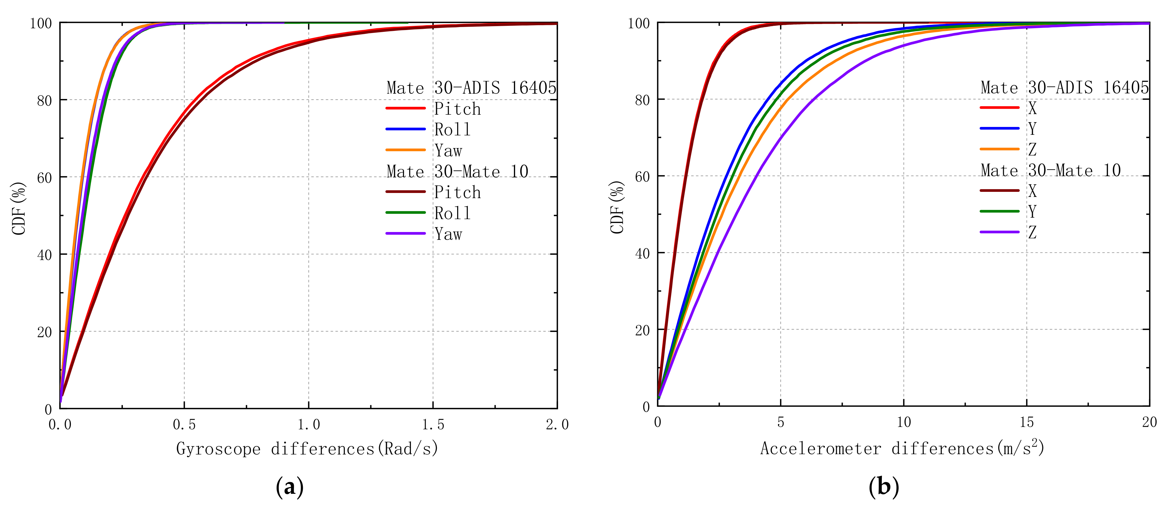
The position estimation accuracy of GNSS measurements depends on the geometry of available GNSS satellite [32]. The PDOP is a factor which indicates the factor of precision of the position with least square estimation (LSE). The Taylor’s series expansion method is used to linearize the pseudorange equation at the approximate receiver position to obtain the difference between the estimated and true receiver positions [33], and the dilution of precision (DOP) measurement matrix can be written as:

$$Q_Z={\left(H^{T}H\right)}^{-1}$$

(1)

where $Q_Z$ is a $4\times 4$ matrix; $H$ is the Jacobian matrix formed with direction cosines from receiver to the satellites. Without the time dilution of precision (TDOP), the PDOP factor is defined as the square root of the trace of the measurement matrix [32]:

$$\mathrm{PDOP}=\sqrt{trace(Q_X)}$$

(2)

where $Q_X$ can be expressed as:

$$Q_X=\left[\begin{array}{ccc}{q}_{11}& q_{12}& q_{13}\\ q_{21}& q_{22}& q_{23}\\ q_{31}& q_{32}& q_{33}\end{array}\right]$$

(3)

The number of GPS and BDS satellites observed by Mate 30 and PDOP values calculated by the formula around the playground twice are shown in Figure 3a. The average number of visible GPS satellites is about 8.1 while that of BDS satellites is about 16.6, and the average PDOP values of GPS and BDS are 1.96 and 1.31, respectively. Although the GNSS signals are slightly degraded due to the trees, the number of visible GPS satellites observed by Mate 30 still fluctuate within a narrow range. For the geodetic receiver, as shown in Figure 3b, it is easy to determine whether the GNSS signals are blocked with the number of visible satellites observed by the geodetic receiver. Meanwhile, although the average number of visible GPS satellites observed by Mate 10 is higher than that of Mate 30, it can be found that the carrier phase measurements of more than half of the visible satellites cannot be logged by Mate 10.

With the GNSS signals slightly degraded due to the trees, as shown in Figure 4b, there are still more than four GPS satellites that can be observed by the Mate 30, as shown in Figure 3a. However, the C/N₀ values of some visible GNSS satellites decrease significantly, as shown in Figure 4a, marked by the red boxes. The C/N₀ is usually used to describe signal noise level in a GNSS receiver, and the value is signal-to-noise ratio (SNR) in 1 Hz width with the unit of dB-Hz.

In Figure 4a, there are 9, 56, and 19 epochs for which the satellite signals of GPS pseudorandom noise (PRN) 17, PRN 19, and PRN 21 cannot be detected in 300 epochs, where the unlock rates are 3.00%, 18.67%, and 6.33%, respectively. The unlock rates of BDS PRN 05, PRN 09, and PRN 21 are 28.00%, 13.33%, and 5.00%, respectively. Both the C/N₀ values of GPS and BDS decrease significantly around 50 epochs and 180 epochs. The average C/N₀ value of GPS in the first 50 epochs is 33.01 dB-Hz, and the average C/N₀ value in the second 50 epochs is 27.20 dB-Hz, which decreases by 17.60%. The average C/N₀ value of BDS in the first 50 epochs is 32.25 dB-Hz, and the average C/N₀ value in the second 50 epochs is 24.67 dB-Hz, which decreases by 23.50%. The maximum C/N₀ values of GPS and BDS are 44 dB-Hz and 39 dB-Hz, while the minimum values are 11 dB-Hz and 9 dB-Hz, respectively.

The second experiment was conducted on the sidewalk where the GNSS signals are significantly degraded due to the buildings and trees on both sides, as shown in Figure 5. The standard deviation (STD) of PDOP values observed by Mate 30 on the sidewalk was 1.17, as shown in Figure 5a, which is 137.96% higher than that of Mate 30 observed on the playground. Compared with the PDOP values observed on the playground in Figure 3b, the STD of PDOP values observed by geodetic receiver and Mate 10 in Figure 5b increased by 201.16% and 247.05%, respectively. Meanwhile, there are 148 and 285 epochs for which the satellite signals of GPS PRN 19 and BDS PRN 05 cannot be detected in 500 epochs, with unlock rates of up to 29.60% and 57.00%, respectively.

In addition, the average C/N₀ value of GPS PRN 19 in the first 50 epochs is 33.55 dB-Hz, and the average C/N₀ value in the second 50 epochs is 15.06 dB-Hz, which decreases by 55.11%. Some studies indicated that the number of carrier phase cycle slips increased significantly with C/N₀ below 30 dB-Hz [8], while some researchers even suggested that the GNSS measurements with C/N₀ below 30 dB-Hz observed by smartphone can be rejected [7,25]. The cutoff C/N₀ value is a convenient method that is suitable for static positioning using smartphones; however, it may not be directly applicable in dynamic mode. In Figure 6a, the average C/N₀ values of GPS and BDS are 28.53 dB-Hz and 27.55 dB-Hz in 500 epochs, respectively, and more than 74.43% of the GPS PRN 19 observations had the C/N₀ below 30 dB-Hz in 500 epochs. Moreover, by comparing GPS PRN 19, PRN 17, and BDS PRN 27, the GNSS satellites with low elevation are more affected by signals being blocked.

2.2. IMU Data

The Huawei Mate 30 integrates an internal IMU chip ICM-20690 developed by Invensense corporation; it is a six-axis motion tracking device which combines a three-axis gyroscope and a three-axis accelerometer in a small $2.5\times 3\times 0.91$ mm package. The low-cost device provides high robustness by supporting 20,000 g shock reliability, while it was also widely used in other smartphones such as Xiaomi Mi 8 and Huawei P40 [29,30]. The initial zero-rate output (ZRO) tolerance of the three-axis gyroscope is ±1°/s and the rate noise spectral density is 0.004°/s/√Hz. The initial tolerance of the three-axis accelerometer is ±40 mg, and the power spectral density is 0.1 mg/√Hz.

The specifications of Analog Devices ADIS16405 are shown in

Table 1. Specifications of Analog Devices ADIS16405. The σ is one sigma (confidence level).

Parameter	Gyroscope	Parameter	Accelerometer
Initial Bias Error (°/s)	±3 (1 σ)	Initial Bias Error (mg)	±50 (1 σ)
In-Run Bias Stability (°/s)	0.007 (1 σ)	In-Run Bias Stability (mg)	0.2 (1 σ)
Angular Random Walk (°/sqrt(h))	2.0 (1 σ)	Velocity Random Walk (m/s/sqrt(h))	0.2 (1 σ)
Rate Noise Density (°/s/sqrt(Hz))	0.05	Noise Density (mg/sqrt(Hz))	0.5

. As shown in Figure 1 for device placement, it should be noted that the x-axis and z-axis of ADIS16405 point to the opposite direction to the y-axis and z-axis of Mate 30, respectively. The ADIS16405 default sample rate setting of 819.2 samples per second (SPS) and the IMU raw data of Mate 30 were recorded with sample rate of 100 SPS. The comparisons of the IMU data from Mate 30 and ADIS16405 on the playground are shown in Figure 7.

Although the IMU data of three-axis gyroscope and three-axis accelerometer recorded by the Mate 30 agree well with the data of ADIS16405, the IMU data of ADIS16405 are smoother than those of Mate 30, which is in line with the comparisons of IMU data recorded by the smartphone Honor Play and the commercial IMU STIM 300 [29]. The mean absolute deviation (MAD) can describe the measuring spread of data, which can be written as:

$$MAD=\frac{1}{n}{\displaystyle \sum _{i=1}^n\left|x_i-\overline{x}\right|}$$

(4)

where $\overline{x}$ is the average value of data. In Figure 7a, The MAD of pitch and roll recorded by Mate 30 are 0.265 rad/s and 0.071 rad/s, which are 18.9% and 4.6% higher than those of ADIS16405, respectively. The MAD of yaw from Mate 30 is 0.078 rad/s, which is almost the same as that of ADIS16405. In Figure 7b, the MAD of x-, y-, and z-axis of the accelerometer recorded by the Mate 30 were 21.1%, 1.2%, and 53.0% higher than those of ADIS16405, respectively. Moreover, the IMU data from Mate 10 were used for comparison, as shown in Figure 8.

The Euclidean metric measure is a widely used distance measure for determining the distance between any two vectors, and the Euclidean distance $\eta$ between two $n$-dimensional vectors is given by:

$$\eta =\sqrt{{\displaystyle \sum _{i=1}^n{\left(x_i-y_i\right)}^2}}$$

(5)

The Euclidean distances of pitch, roll, and yaw between Mate 30 and ADIS16405 are 83.30, 20.66, and 20.40, respectively. However, in Figure 8a, the Euclidean distances between Mate 30 and Mate 10 are 86.86, 25.69, and 24.16, respectively. Meanwhile, in Figure 8b, the average Euclidean distance of the accelerometer between Mate 30 and Mate 10 is 632.05, which is also higher than that between Mate 30 and ADIS16405.

The CDF of three-axis gyroscope and accelerometer differences are shown in Figure 9. The pitch, roll, and yaw differences between Mate 30 and ADIS16405 are lower than those between Mate 30 and Mate 10 within the same percentile in Figure 9a, and the differences are 3.39, 0.95, and 0.54 rad/s within one sigma, respectively. Meanwhile, the CDF of three-axis accelerometer differences between Mate 30 and ADIS16405 are also lower than those between Mate 30 and Mate 10 within the same percentile in Figure 9b. Compared with the gyroscope and accelerometer differences between Mate 30 and Mate 10, the IMU measurements from Mate 30 match slightly better with those from ADIS16405.

3. Multi-GNSS PPP/INS Mathematical Model

The researchers recorded that some smartphones such as Mi 8 received above four satellites with L5/E5 band for only about 13 h over a 24 h collection [10], and there are only a few Galileo satellites observed by smartphones such as Huawei Mate 30 that can be logged with dual-frequency observations [8]. It is difficult to conduct dual-frequency PPP with an ionosphere-free combined model [12,34] especially in the GNSS-degraded environment. Therefore, the uncombined PPP model for dual-frequency GNSS observations of smartphones was used in this experiment, and the flow chart of the GNSS PPP/INS integrated navigation scheme is shown in Figure 10.

The PPP/INS integrated navigation scheme for smartphones mainly consists of uncombined PPP model and INS model. The initial absolute position of the smartphone was provided by GNSS PPP solutions, and the initial alignment of PPP/INS was conducted in dynamic mode. Meanwhile, the stochastic model is composed of GNSS step function variances depending on C/N₀, and the RKF is applied to parameter estimation. The specific mathematical models are as follows.

3.1. Uncombined PPP Model

The GNSS observation equations for pseudorange and carrier phase between receiver and satellite are given by the following:

$$P_i^s={\rho }^s+cd{t}_r+cd{t}_D^s-cd{t}^s+T^s+\frac{f_1^2}{f_i^2}{I}^s+B_{P_i}^{r,s}-B_{P_i}^s+{\epsilon }_{{}_{P_i}}^{}$$

(6)

$$L_i^s={\rho }^s+cd{t}_r+cd{t}_D^s-cd{t}^s+T^s-\frac{f_1^2}{f_i^2}{I}^s-{\lambda }_i^s{N}_i^s+B_{L_i}^{r,s}-B_{L_i}^s+{\epsilon }_{L_i}^{}$$

(7)

where $P$ is pseudorange measurements, and $L$ is carrier phase measurements scaled to distance; the superscript $s$ denotes satellite system, and the subscript $i$ denotes frequency; $\rho$ is the geometric range between the receiver and satellite; $c$ is the speed of light in vacuum, and $d{t}_r$ is receiver clock error; $d{t}_D^s$ is the time bias between $s$ satellite system and GPS; $d{t}^Q$ is satellite clock error; $T$ is tropospheric delay; $f_i$ is the frequency of $L_i$, and $I$ is ionospheric delay of $L_1$; ${\lambda }_i$ is the wavelength of $f_i$,$N_i$ is the integer ambiguity of $L_i$ in cycle; the symbols $B_{P_i}^r$, $B_{L_i}^r$, $B_{P_i}^s$, and $B_{L_i}^s$ are code and phase hardware delay of receiver and satellite, respectively, and the $\epsilon$ terms are unmodeled errors, including code and phase multipath effect and measurement random noise.

According to the studies on GNSS signal characteristics of smartphones such as Huawei P10, P20, and Mate 30, the carrier-to-noise weighting should be used for low-cost GNSS receivers instead of elevation-dependent weighting [7,8,15]. Based on the formula [35,36] that expresses the phase variance ${\sigma }_S^2$ in $\mathrm{m}{\mathrm{m}}^2$ as a function of the measured C/N₀ values, and with reference to elevation-dependent weighting method, the GNSS step function variance of smartphone can be given as:

$${\sigma }_s^2(\mathrm{C}/{\mathrm{N}}_0)=\left\{\begin{array}{ll}{C}_s\cdot {10}^{\frac{-(\mathrm{C}/{\mathrm{N}}_0\mathrm{measured})}{10}}\hfill & \mathrm{C}/{\mathrm{N}}_0>\alpha \hfill \\ C_s\cdot {10}^{\frac{-(\mu \cdot \mathrm{C}/{\mathrm{N}}_0\mathrm{measured})}{10}}\hfill & \mathrm{C}/{\mathrm{N}}_0\le \alpha ,\mu \in \left(0,1\right)\hfill \end{array}\right.$$

(8)

and

$$C_s=B_s{\left[\frac{\lambda }{2\pi }\right]}^2$$

(9)

where $\alpha$ is the threshold value of C/N₀; $\mu$ denotes coefficient of C/N₀ which can be determined by the gross GNSS measurements noise below the threshold value; $B_S$ is the carrier tracking loop bandwidth (Hz), and the effect of the oscillator stability on the phase variances is considered negligible. Due to the lack of bandwidth information, the constant values obtained by fitting phase variance and C/N₀ variance are usually used as the parameters $C_S$.

By using Equations (6) and (7), the error equation of GNSS observation is given directly as:

$$V=H\cdot X+l$$

(10)

where $V$ is measurement residual, and $H$ is the coefficient matrix. The GNSS basic parameters can be written as:

$$X_{\mathrm{GNSS}}=\left[x,\hspace{1em}y,\hspace{1em}z,\hspace{1em}cd{t}_r,\hspace{1em}cd{t}_D^B,\hspace{1em}T,\hspace{1em}{\hat{I}}_1,\hspace{1em}{\hat{N}}_1^G\hspace{1em}{\hat{N}}_5^G\hspace{1em}{\hat{N}}_1^B\right]$$

(11)

where $x$, $y$, $z$ denote three-dimensional coordinates of the receiver, $d{t}_D^B$ is BDS system time bias, ${\hat{I}}_1$ denotes ionospheric delay of $L_1$, ${\hat{N}}_1^G$, ${\hat{N}}_5^G$, and ${\hat{N}}_1^B$ are the integer ambiguity parameters of GPS and BDS, respectively.

3.2. MEMS–INS Model

Commonly used coordinate systems in inertial navigation mainly include inertial frame (i-frame), Earth-centered Earth-fixed frame (e-frame), body frame (b-frame), and navigation frame (n-frame). With the dead reckoning algorithm, the dynamic equation of INS in e-frame can be summarized as [37]:

$$\left(\begin{array}{c}{\dot{r}}_{\mathrm{INS}}^e\\ {\dot{v}}_{\mathrm{INS}}^e\\ {\dot{C}}_b^e\end{array}\right)=\left(\begin{array}{c}{v}_{\mathrm{INS}}^e\\ C_b^e{f}_{ib}^b-2{\mathsf{\Omega }}_{ie}^e{v}_{\mathrm{INS}}^e+g^e\\ C_b^e{\mathsf{\Omega }}_{eb}^b\end{array}\right)$$

(12)

where $r_{\mathrm{INS}}^e$ and $v_{\mathrm{INS}}^e$ denote the position and velocity vectors of the IMU in the e-frame, respectively; $C_b^e$ denotes the direction cosine matrix from b-frame to e-frame, and $f_{ib}^b$ denotes the specific force vector of e-frame with respect to i-frame in the e-frame; ${\mathsf{\Omega }}_{ie}^e$ denotes the skew symmetric matrix of the earth rotation vector of ${\omega }_{ie}^e$ relative to i-frame, expressed in e-frame; $g^e$ denotes the gravity vector in the e-frame; ${\mathsf{\Omega }}_{eb}^b$ denotes the skew symmetric matrix of ${\omega }_{eb}^b$, and ${\omega }_{eb}^b$ can be written as:

$${\omega }_{eb}^b={\omega }_{ei}^b+{\omega }_{ib}^b={\omega }_{ib}^b-{\omega }_{ie}^b={\omega }_{ib}^b-C_e^b{\omega }_{ie}^e$$

(13)

where ${\omega }_{ib}^b$ denotes gyroscope angular velocity, $C_e^b$ denotes the inverse matrix of $C_b^e$.

By using the dynamic equation, the error state model of INS can be expressed as [38]:

$$\left(\begin{array}{c}\delta {\dot{r}}_{\mathrm{INS}}^e\\ \delta {\dot{v}}_{\mathrm{INS}}^e\\ {\dot{\phi }}^e\end{array}\right)=\left(\begin{array}{c}\delta v_{\mathrm{INS}}^e\\ -2{\mathsf{\Omega }}_{ie}^e\delta v_{\mathrm{INS}}^e+\left[\left(C_b^e{f}_{ib}^b\right)\times \right]{\phi }^e-C_b^e\delta f_{ib}^b\\ -{\mathsf{\Omega }}_{ie}^e{\phi }^e+C_b^e\delta {\omega }_{ib}^b\end{array}\right)$$

(14)

where $\left[\left(C_b^e{f}_{ib}^b\right)\times \right]$ denotes the skew symmetric matrix of $\left(C_b^e{f}_{ib}^b\right)$. The errors of specific force and gyroscope angular velocity can be written as follows:

$$\delta f_{ib}^b=\delta b_a+{\epsilon }_a$$

(15)

$$\delta {\omega }_{ib}^b=\delta b_g+{\epsilon }_g$$

(16)

Then, the linearized state equation of INS can be expressed as:

$$\left[\begin{array}{c}\delta {\dot{r}}_{\mathrm{INS}}^e\\ \delta {\dot{v}}_{\mathrm{INS}}^e\\ {\dot{\phi }}^e\\ \delta {\dot{b}}_a\\ \delta {\dot{b}}_g\end{array}\right]=\left[\begin{array}{ccccc}0& I& 0& 0& 0\\ 0& -2{\mathsf{\Omega }}_{ie}^e& \left[\left(C_b^e{f}_{ib}^b\right)\times \right]& -C_b^e& 0\\ 0& 0& -{\mathsf{\Omega }}_{ie}^e& 0& C_b^e\\ 0& 0& 0& 0& 0\\ 0& 0& 0& 0& 0\end{array}\right]\left[\begin{array}{c}\delta r_{\mathrm{INS}}^e\\ \delta v_{\mathrm{INS}}^e\\ {\phi }^e\\ \delta b_a\\ \delta b_g\end{array}\right]+\left[\begin{array}{cc}0& 0\\ -C_b^e& 0\\ 0& C_b^e\\ 0& 0\\ 0& 0\end{array}\right]\left[\begin{array}{c}{\epsilon }_a\\ {\epsilon }_b\end{array}\right]$$

(17)

where $\delta r_{\mathrm{INS}}^e$, $\delta v_{\mathrm{INS}}^e$, and ${\phi }^e$ denote the position, velocity, and attitude error vector in e-frame; $\delta b_a$ and $\delta b_g$ denote the bias errors of accelerometer and gyroscope, respectively; ${\epsilon }_a$ and ${\epsilon }_g$ denote the processing noise vectors of accelerometer and gyroscope biases, respectively.

3.3. Uncombined PPP/INS Coupled Model

Considering the bias error and noise of low-cost IMU, the initial alignment of INS is usually conducted with dynamic mode. The pitch and roll angle are calculated by accelerometer of IMU:

$$\varphi =-sign(f_D^n)si{n}^{-1}\left(\frac{f_E^n}{g}\right)$$

(18)

$$\theta =sign(f_D^n)si{n}^{-1}\left(\frac{f_N^n}{g}\right)$$

(19)

where $\varphi$ and $\theta$ are pitch and roll angle, respectively; $f^n$ is the specific force vector in the n-frame; $E$, $N$, and $D$ denote the east, north, and down directions, respectively; $\mathrm{g}$ is the gravity vector. With the roll angle in the plane set to zero approximately, the approximate pitch and yaw angle are solved by GNSS with the information of location and speed, which can be expressed as [29]:

$$\varphi =ta{n}^{-1}\left(\frac{v_D}{\sqrt{v_N^2+v_E^2}}\right)$$

(20)

$$\psi =ta{n}^{-1}\left(\frac{v_E}{v_N}\right)$$

(21)

Moreover, the PPP/INS model coupled with the data of the MEMS module, such as ADIS16405 and the GNSS observations from smartphones, should unify the measurements to the same reference frame using the level arm. The conversion relation with the level arm correction vector $l^b$ calculated by the IMU geometrical center and the GNSS antenna phase center can be expressed as [37]:

$$r_{\mathrm{GNSS}}^e=r_{\mathrm{INS}}^e+C_b^e{l}^b$$

(22)

$$v_{\mathrm{GNSS}}^e=v_{\mathrm{INS}}^e+C_b^e{\mathsf{\Omega }}_{ib}^b{l}^b-{\mathsf{\Omega }}_{ie}^e{C}_b^e{l}^b$$

(23)

where $r_{\mathrm{GNSS}}^e$ and $v_{\mathrm{GNSS}}^e$ denote the position and velocity vectors of the GNSS antenna phase center in the e-frame, respectively; ${\mathsf{\Omega }}_{ib}^b$ denotes the skew symmetric matrix of ${\omega }_{ib}^b$. In addition, the state covariance matrix, system noise matrix and state transition matrix should be adjusted. Combining state vector $X_{\mathrm{GNSS}}$ in Equation (11), the dynamics model of PPP/INS can be expressed as:

$$\left[\begin{array}{c}{z}_r^e\\ z_v^e\end{array}\right]=\left[\begin{array}{c}{r}_{\mathrm{GNSS}}^e\\ v_{\mathrm{GNSS}}^e\end{array}\right]-\left(\left[\begin{array}{c}{r}_{\mathrm{INS}}^e\\ v_{\mathrm{INS}}^e\end{array}\right]+\left[\begin{array}{c}{C}_b^e{l}^b\\ C_b^e{\mathsf{\Omega }}_{eb}^b{l}^b\end{array}\right]\right)$$

(24)

and the basic parameters of PPP/INS dynamic equation can be written as:

$$X_{\mathrm{PPP}/\mathrm{INS}}=\left[\begin{array}{ccccc}\widehat{r},& \widehat{v},& \widehat{\phi },& {\widehat{b}}_a,& {\widehat{b}}_g\end{array}\right]$$

(25)

while the coefficient matrix can be expressed as:

$$H_{\mathrm{PPP}/\mathrm{INS}}=\left[\begin{array}{ccccc}-I_{3\times 3}& 0& C_b^e{l}^b& 0& 0\\ 0& -I_{3\times 3}& C_b^e{\mathsf{\Omega }}_{eb}^b{l}^b& 0& 0\end{array}\right]$$

(26)

3.4. Robust Kalman Filter Parameter Estimation Model

To reduce the effects of measurement outliers on smartphones positioning, the robust Kalman filter method is used for parameter estimation to balance the contribution of normal and abnormal observations with equivalent variance matrix. Based on the nonlinear extended Kalman filter dynamic and observation models, the formula of robust Kalman gain matrix ${\overline{K}}_k$ can be written as [39]:

$${\overline{K}}_k=P_k^{-}{H}_k^T{(H_k{P}_k^{-}{H}_k^T+{\overline{R}}_k)}^{-1}$$

(27)

where $P_k^{-}$ denotes the state covariance matrix, and $H_k$ denotes the coefficient matrix. With the robust M estimation principle, the equivalent covariance matrix is ${\overline{R}}_k$ instead of the original covariance $R_k$, which can be expressed as [40]:

$${\overline{R}}_k=\frac{R_k}{{\gamma }_i}$$

(28)

where ${\gamma }_i$ denotes the variance inflation factor. Based on the institute of geodesy and geophysics (IGG) III weighting function, the reduction factor of the weight elements could be chosen as [41]:

$${\gamma }_i=\left\{\begin{array}{ll}1& \left|{\overline{v}}_i\right|\le k_0\\ \frac{k_0}{\left|{\overline{v}}_i\right|}{\left(\frac{k_1-\left|{\overline{v}}_i\right|}{k_1-k_0}\right)}^2& k_0<\left|{\overline{v}}_i\right|\le k_1\\ 0& \left|{\overline{v}}_i\right|>k_1\end{array}\right.$$

(29)

where $k_0$ and $k_1$ are thresholds commonly used as 1.5–3.0 and 3.0–8.0, respectively; ${\overline{v}}_i$ denotes a standardized residual, as follows [42]:

$${\overline{v}}_i=\frac{v_i}{\sqrt{{\hat{\sigma }}_0^2{Q}_{vi}}}$$

(30)

where $v_i$ denotes the residual of measurements, and $Q_{vi}$ denotes corresponding variance, ${\hat{\sigma }}_0^2$ denotes the unit weight variance estimated by generalized least squares.

$${\hat{\sigma }}_0^2=\frac{{\xi }^T{Q}_{\xi }^{-1}\xi }{n}$$

(31)

where $\xi$ denotes predicted residual vector (innovations), $Q_{\xi }$ denotes the corresponding covariance matrix as follows:

$$Q_{\xi }=R_k+H_k{P}_k^{-}{H}_k^T$$

(32)

The updated state correction vector and error covariance of the robust Kalman filter can be expressed as:

$${\hat{X}}_k={\hat{X}}_{\overline{k}}+{\overline{K}}_k(L_k-H_k{\hat{X}}_{\overline{k}})$$

(33)

$$P_k=[I-{\overline{K}}_k{H}_k]P_k^{-}{[I-{\overline{K}}_k{H}_k]}^T+{\overline{K}}_k{\overline{R}}_k{\overline{K}}_k^T$$

(34)

4. Experiment and Result

The PPP/INS positioning experiments of smartphones were conducted using GNSS observations including L1/L5 of GPS and B1 of BDS from smartphones and IMU data from smartphones and triaxial inertial sensor ADIS16405. The products, such as precise satellite orbit and clock, final global ionospheric map (GIM), and differential code bias (DCB), were provided by the IGS data center. The hydrostatic troposphere error was corrected with the Saastamoinen model [43], and the zenith delay of the wet troposphere was estimated as a parameter. Moreover, the other effects, such as Earth tide, relativity, and Sagnac, were modeled and corrected sufficiently. The cutoff elevation of satellites was 15 degrees, and the position was initialized from standard single point positioning (SPP) using pseudorange on the L1 frequency with a variance of 60² (m²). The receiver clock was initialized with a variance of 60² (m²) per epoch, and other parameters, such as the integer ambiguities of carrier phase, were usually initialized at the beginning and estimated as a float solution.

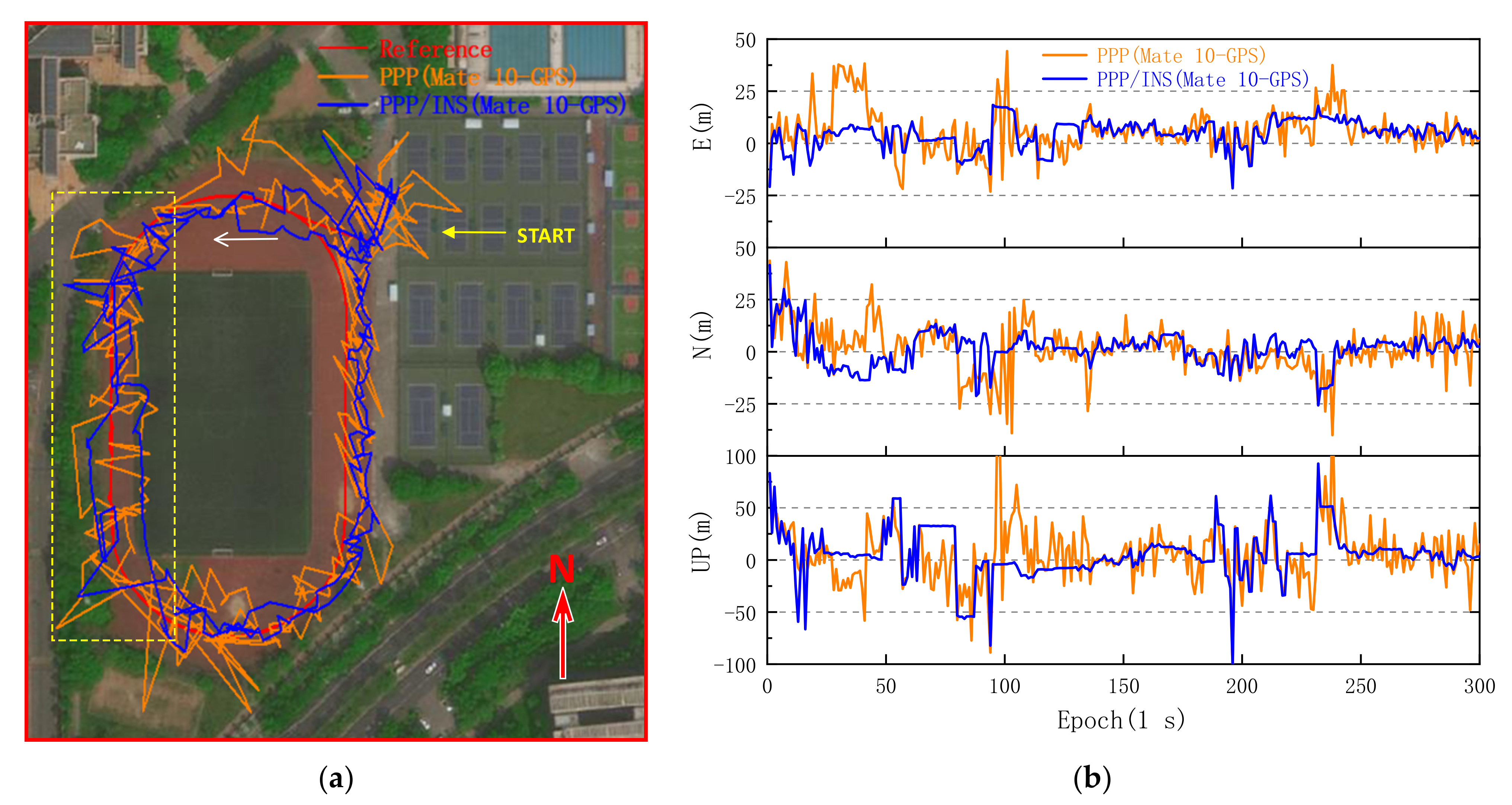
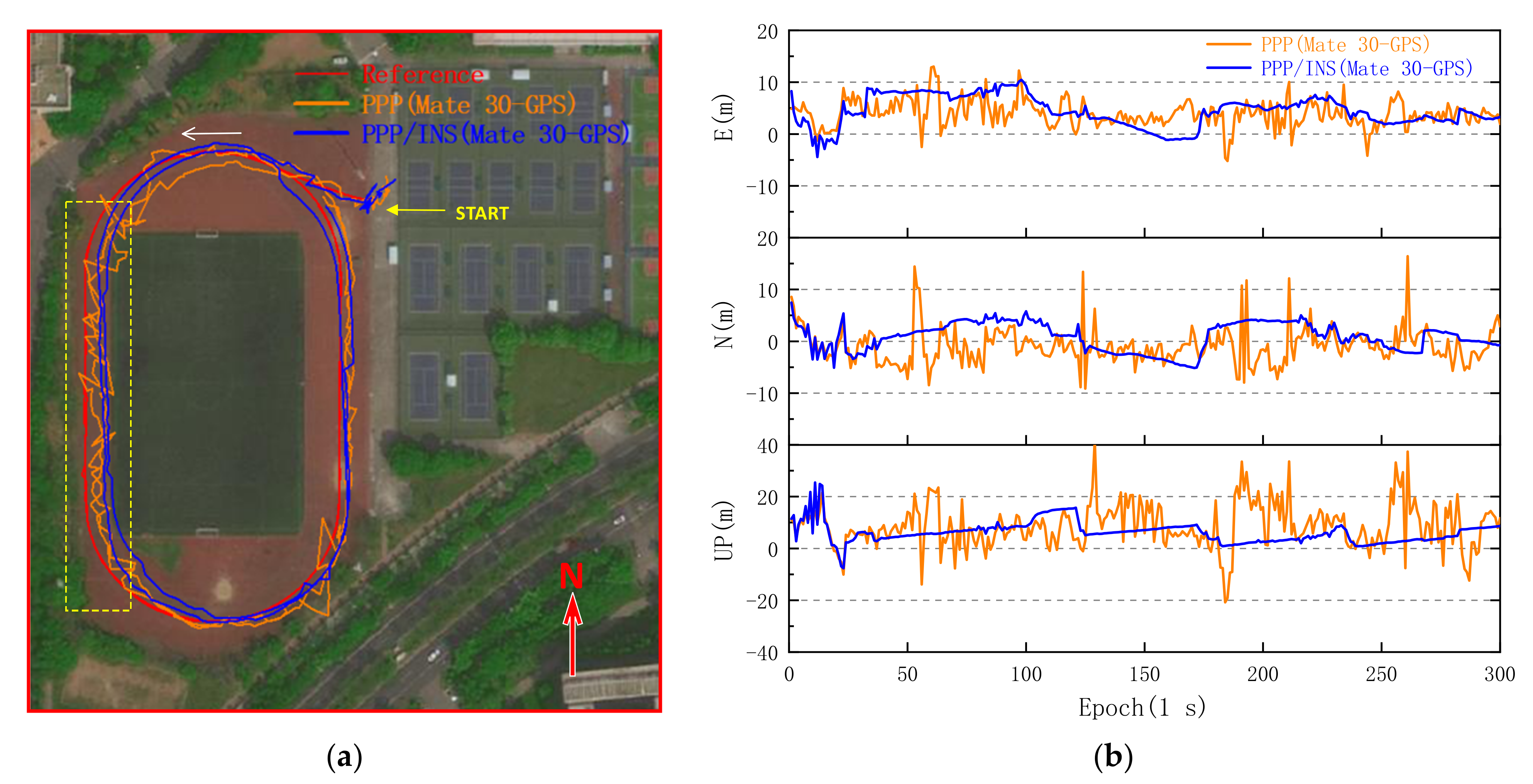
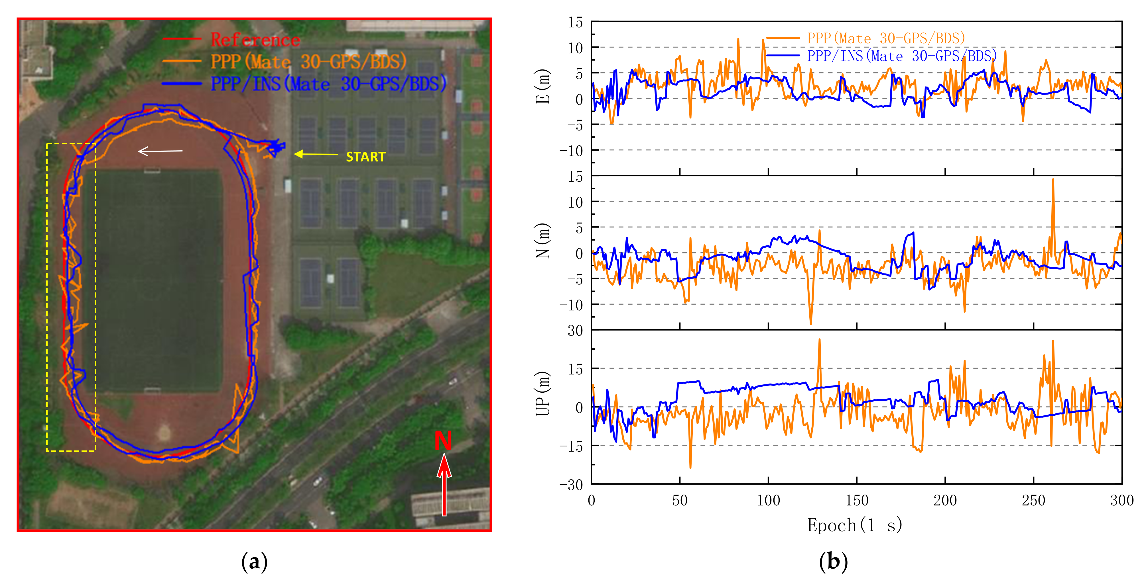
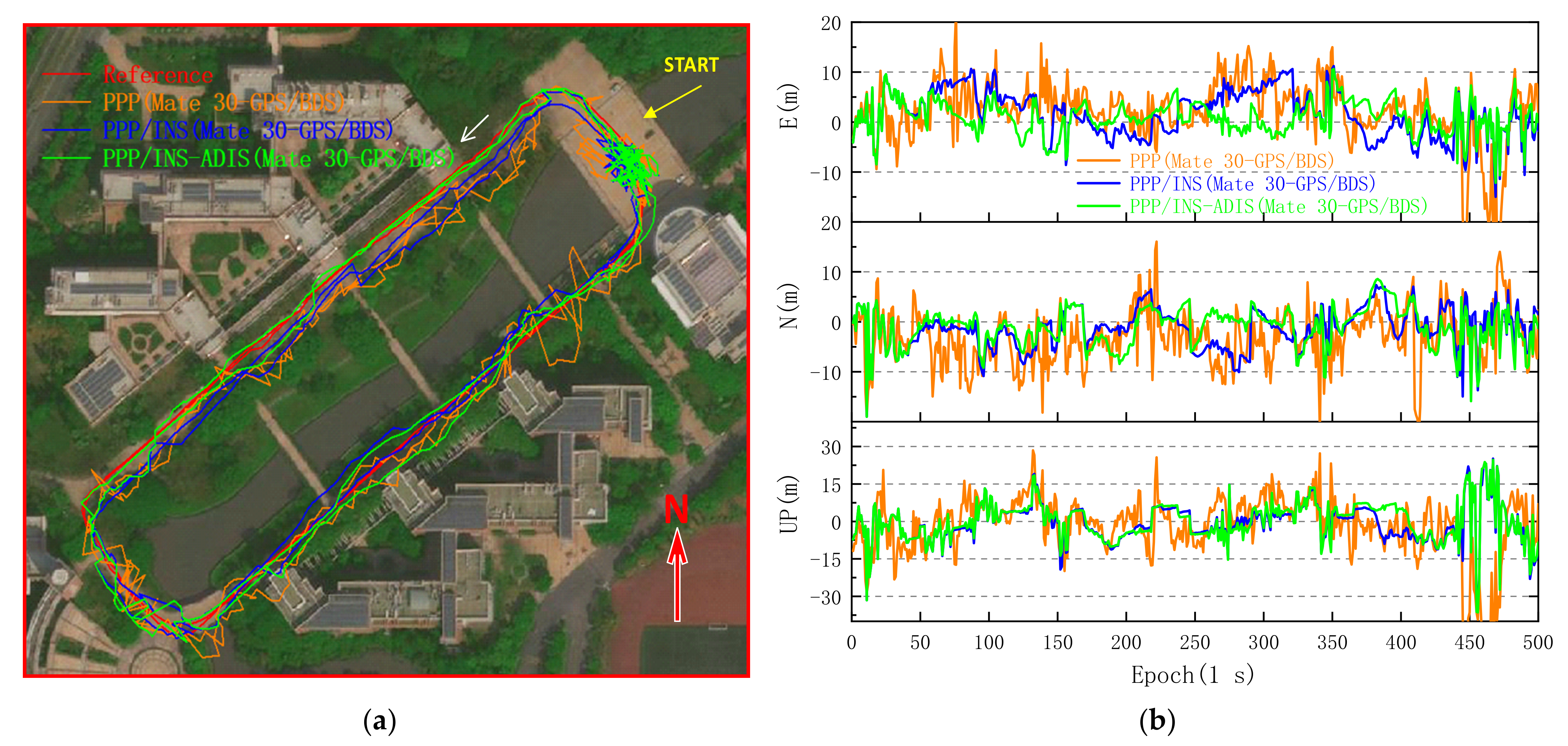
4.1. PPP/INS Solutions on the Playground and Sidewalk

While the pitch and roll angle were calculated by accelerometer, the yaw angle of smartphones was estimated by position and speed provided by GNSS solutions for PPP/INS initial alignment in dynamic mode. The INS parameters would be initialized while both the velocity of the receiver and the PDOP of the GNSS reached corresponding thresholds. Meanwhile, considering the convergence velocity and precision of smartphones PPP initialization, the yaw angle is directly estimated by the geodetic receiver with differential positioning during INS initial alignment in the experiments. Moreover, some reference coordinates which cannot be outputted by the geodetic receiver with GNSS integer ambiguities estimated as a fix solution were estimated by the post-processing fitting method. The conventional PPP method adopted the standard Kalman filter parameter estimation model while the robust Kalman filter was used in the PPP/INS coupled model, and both adopted the C/N₀-dependent stochastic model. The PPP and PPP/INS positioning trajectories of Huawei Mate 10 are shown in Figure 11a, and the corresponding positioning errors in terms of east, north, and up directions are shown in Figure 11b.

In Figure 11a, the positioning errors of single-frequency GPS PPP of the Huawei Mate 10 show a significant fluctuation at the beginning even in the open area, and then the smartphone enters the area marked by the yellow box successively in about 50 epochs and 180 epochs. In Figure 11b, the RMS of GPS PPP/INS horizontal errors is 11.293 m, which decreases by 32.24% compared with that of GPS PPP horizontal errors, and the RMS of PPP/INS vertical errors is 23.717 m, which decreases by 19.63% compared with that of GPS PPP vertical errors. However, although the positioning accuracy of the Huawei Mate 10 is improved with INS, its absolute positioning accuracy is still closely related to positioning accuracy of the smartphone PPP. For the early single-frequency smartphones such as Mate 10, an amount of raw carrier phase measurements cannot be logged due to many cycle slips in GNSS-degraded environments, and the weak positioning performance makes it difficult to meet the requirements of a high-precision location service even in the open area. In contrast, the dual-frequency smartphone Mate 30 has significantly better positioning performance, as shown in Figure 12. The RMS of Mate 30 GPS PPP horizontal errors can reach 5.996 m in the same environment.

From Figure 12b, although the Mate 30 GPS PPP/INS maximum horizontal positioning error decreases by 32.08% from 16.407 to 11.144 m, the horizontal positioning accuracy did not improve significantly with INS, and the RMS of Mate 30 PPP/INS horizontal errors is 6.033 m which is almost the same as that of PPP. Meanwhile, in Figure 12a, it can be found that the trajectory of PPP/INS positioning is still flat while the smartphone is in the area marked by the yellow box, but the offset is also increasing. However, the RMS of GPS PPP/INS vertical positioning errors decreases by 39.80% from 12.274 to 7.389 m, and the RMS of three-dimensional positioning errors is 9.539 m. Then, the BDS observations of Mate 30 were used in the GNSS PPP/INS experiment, and the results are shown in Figure 13.

Compared with Figure 12a, the offset of trajectory was significantly improved in Figure 13a. In

Table 2. RMS of GNSS PPP and PPP/INS positioning error using smartphones on the playground. Dir denotes direction. G and B denote GPS and BDS, respectively. H, V, and 3D denote horizontal, vertical, and three-dimensional.

	Smartphone Kinematic Positioning Error RMS (m)
Dir	Huawei Mate 10		Huawei Mate 30
	G(PPP)	G(PPP/INS)	G(PPP)	G(PPP/INS)	GB(PPP)	GB(PPP/INS)
E	12.157	8.112	4.732	5.318	3.666	2.546
N	11.403	8.304	3.682	2.849	3.920	2.521
H	16.668	11.293	5.996	6.033	5.367	3.583
V	29.509	23.717	12.274	7.389	7.359	5.546
3D	33.891	26.269	13.660	9.539	9.108	6.603

, the RMS of Mate 30 GPS/BDS PPP/INS horizontal errors decreases by 33.24% from 5.367 to 3.583 m, and the maximum horizontal positioning error decreases from 15.041 to 7.294 m. The RMS of Mate 30 GPS/BDS PPP/INS vertical errors decreases by 24.64% from 7.359 to 5.546 m. Previously, the average C/N₀ value observed on the west side of the playground was significantly lower than that on the east side, as shown in Figure 4a. Comparing the PPP solutions on the west and east sides of the playground, the RMS of Mate 30 GPS/BDS PPP horizontal errors on the west side is 6.515 m, which is 27.17% higher than the 5.123 m on the east side.

However, based on the INS-aided and RKF parameter estimation model, the RMS of Mate 30 GPS/BDS positioning horizontal errors on the west side of the playground decreases by 41.21% to 3.830 m, and the RMS of Mate 30 GPS/BDS positioning horizontal errors on the east side of the playground can reach 3.073 m. Subsequently, the IMU data of ADIS16405 were used with Huawei Mate 30 in the experiment on the sidewalk, and the GNSS PPP and PPP/INS solutions are shown in Figure 14.

Although the GNSS signals are significantly degraded due to the buildings and trees on both sides in Figure 14a, the PPP solutions of Mate 30 still can be outputted with GPS and BDS. However, compared with the PPP solutions on the playground, the RMS of PPP horizontal and vertical errors increases to 9.200 and 13.389 m, respectively. In Figure 14b, the RMS of PPP/INS horizontal errors decreases by 29.53% to 6.483 m, and the RMS of PPP/INS vertical errors decreases by 41.98% from 13.389 to 7.768 m. Meanwhile, compared with the positioning trajectories between PPP/INS and PPP/INS–ADIS, it can be found that the trajectory of PPP/INS–ADIS fits more closely to the reference trajectory, especially on the northwest side. As shown in

Table 3. RMS of GPS/BDS PPP and PPP/INS positioning errors using Huawei Mate 30 on the sidewalk.

Direction	Huawei Mate 30 Kinematic Positioning Error RMS (m)
	GB(PPP)	GB(PPP/INS)	GB(PPP/INS–ADIS)
E	6.589	4.903	3.470
N	6.420	4.241	4.054
H	9.200	6.483	5.336
V	13.389	7.768	7.859
3D	16.245	10.118	9.499

, the RMS of PPP/INS–ADIS horizontal errors is 5.336 m, which is lower than that of PPP/INS, and the RMS of PPP/INS–ADIS vertical errors is approximate to that of PPP/INS.

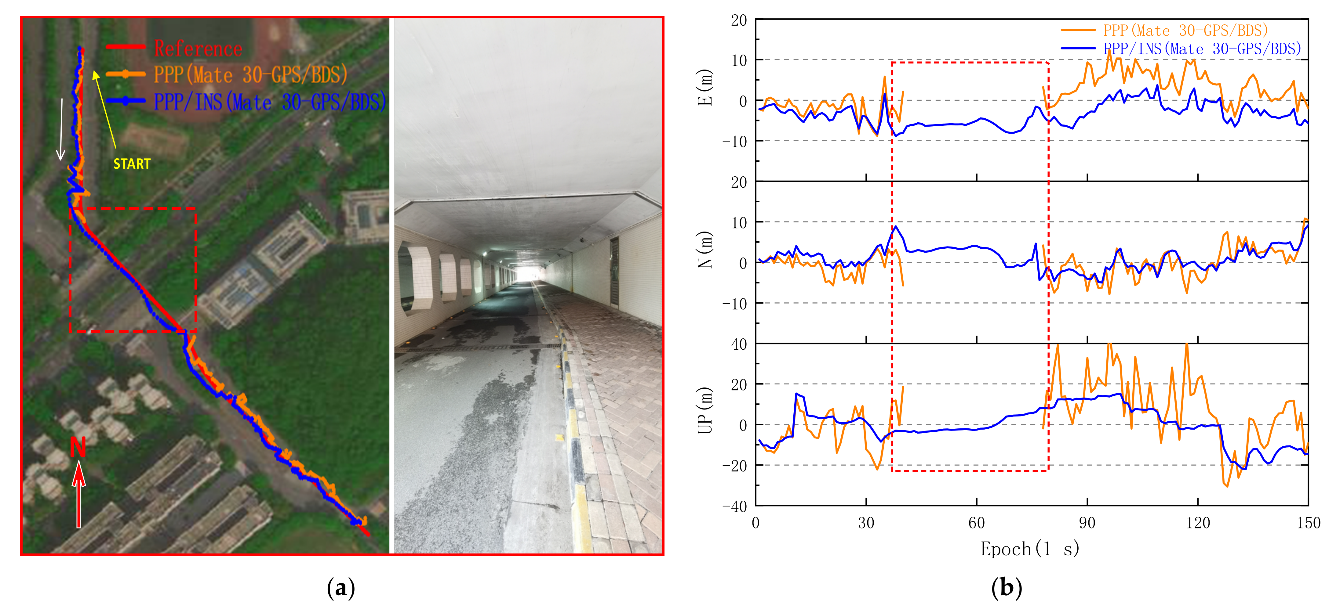
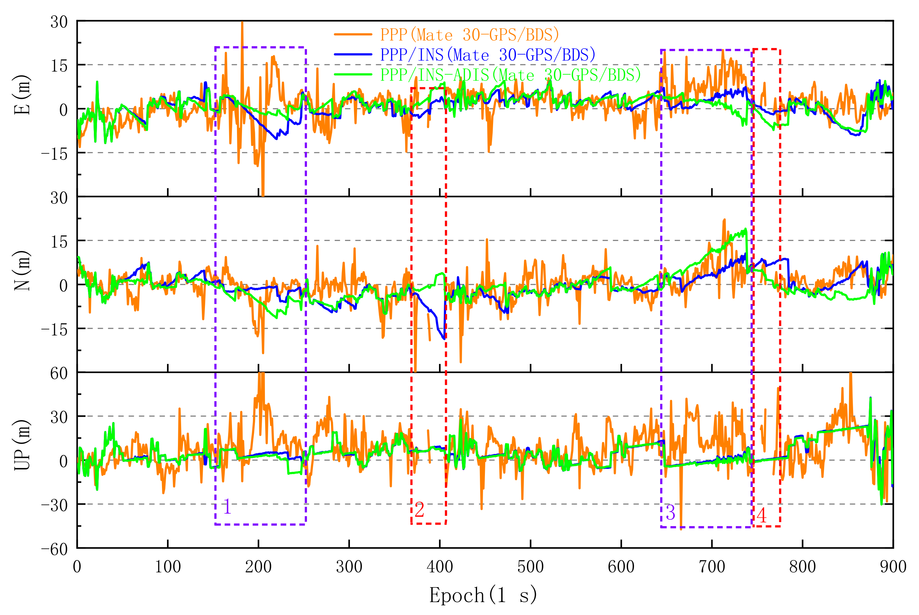
4.2. PPP/INS Solutions for Tunnel and Long Trajectory

Considering that few GNSS satellites signals can be observed by smartphones in some areas such as tunnels, the solutions of the current epoch would be output by INS when the number of satellites could not meet the requirements of GNSS positioning, and other parameters, such as ambiguity, are usually initialized at the beginning, which are the same as before. As shown in Figure 15a, the experiment was conducted in a tunnel shown on the right with a length of about 80 m, and the vertical drop is more than 10 m. The trajectories of Mate 30 GPS/BDS PPP and PPP/INS solutions are shown on the left, and the gaps between the positioning points are preserved in the trajectory.

In fact, the GNSS satellite signals were blocked gradually before the smartphone entered the tunnel, the PDOP value of GNSS satellites increased gradually, and the horizontal and vertical errors were shown to fluctuate significantly for 25 to 40 epochs in Figure 15b. From 41 to 77 epochs, the number of GNSS satellites observed by Mate 30 was insufficient to meet the requirement of the PPP method. Nevertheless, the position of the smartphone can still be obtained continuously with the PPP/INS coupled method while inside the tunnel, and the horizontal deviation from the reference point is more than 8 m at 29 epochs. Then, the positioning points of PPP/INS gradually approach the reference trajectory after leaving the tunnel. The RMS of horizontal deviation in the tunnel is 6.700 m, and the maximum horizontal and vertical deviation are 8.139 and 7.996 m, respectively. Compared with the RMS of PPP/INS horizontal errors from 1 to 40 epochs, the RMS of PPP/INS horizontal errors in the tunnel increases only 21.99%. Meanwhile, it should be noted that the deviation will increase significantly with the further increase of the length of tunnel. Finally, a long trajectory experiment with PPP, PPP/INS, and PPP/INS–ADIS was conducted, and the trajectories are shown in Figure 16.

In the areas marked by purple boxes 1 and 3, it can be found that the trajectory of GPS/BDS PPP is not smooth, and the maximum horizontal errors of GPS/BDS PPP in the areas even reached 49.813 m and 27.627 m, respectively. This can be attributed to the measurement residuals of some satellites with low signal quality, which belong to outliers and are not eliminated in the process of iteration. With the INS-aided and RKF parameter estimation model, as shown in Figure 17, the maximum horizontal errors of GPS/BDS PPP/INS in the areas marked by purple boxes 1 and 3 are 20.662 and 8.933 m, which are decreased by 58.52% and 67.67%, respectively.

As shown in

Table 4. The RMS of PPP, PPP/INS, and PPP/INS positioning errors using Huawei Mate 30 on the areas marked by purple boxes 1 and 3.

Direction	Huawei Mate 30 GPS/BDS Kinematic Positioning Error RMS (m)
	150–250 (Epochs)			650–750 (Epochs)
	PPP	PPP/INS	PPP/INS–ADIS	PPP	PPP/INS	PPP/INS–ADIS
E	9.837	5.252	2.267	9.072	3.532	3.788
N	5.799	2.417	5.998	7.258	4.860	6.574
H	11.419	5.782	6.412	11.618	6.008	7.587
V	23.190	4.507	5.083	19.446	2.784	7.498
3D	25.849	7.331	8.183	22.652	6.622	10.667

, compared with PPP solutions, the RMS of PPP/INS horizontal errors in the area marked by purple box 1 decreases by 49.37% from 11.419 to 5.782 m, and the RMS of PPP/INS horizontal errors in the area marked by purple box 3 decreases by 48.29% from 11.618 to 6.008 m. Meanwhile, the RMS of PPP/INS vertical errors also decreases significantly. In the area marked by red box 2, as shown in Figure 16, the deviations on the south direction between the trajectories of PPP/INS and reference increased rapidly after the GNSS signals were blocked, which can be caused by the scarcity of GNSS satellites before. Meanwhile, it can be found that the southward error of PPP is higher than 30 m in 373 epochs, as shown in Figure 17. However, compared with the trajectory of PPP/INS, the deviations of trajectory between PPP/INS–ADIS and reference are lower. In the area marked by red box 4, the deviations of trajectory of PPP/INS are approximate to those of PPP/INS–ADIS. For the long trajectory experiment, the RMS of PPP/INS and PPP/INS–ADIS horizontal errors are 6.01 and 5.73 m, respectively, which are significantly lower than those of conventional PPP.

Therefore, with the higher reliability of initial alignment in dynamic mode and RKF parameter estimation model with equivalent variance matrix, some adverse factors, such as the effects of multipath, noise level, and observations gaps, related to GNSS signal quality of smartphones under GNSS-degraded environments were overcome to some extent. The convergence efficiency of the PPP/INS model is enhanced and the trajectory deviation of the smartphone can remain stable in some areas, such as tunnels, when GNSS signals are blocked.

5. Conclusions

In this study, we proposed an IMU-aided uncombined PPP coupled mathematical model that integrated IMU data and GNSS observations from smartphones to enhance the positioning performance of smartphones under GNSS-degraded environments. The GNSS measurements observed by the dual-frequency smartphone Huawei Mate 30 integrated Hi1103 chipset and the single-frequency smartphone Huawei Mate 10 integrated BCM47531 chipset, and the data of IMU from the smartphones and triaxial inertial sensor ADIS16405, were used in several experiments. The main conclusions are summarized as follows:

(1)

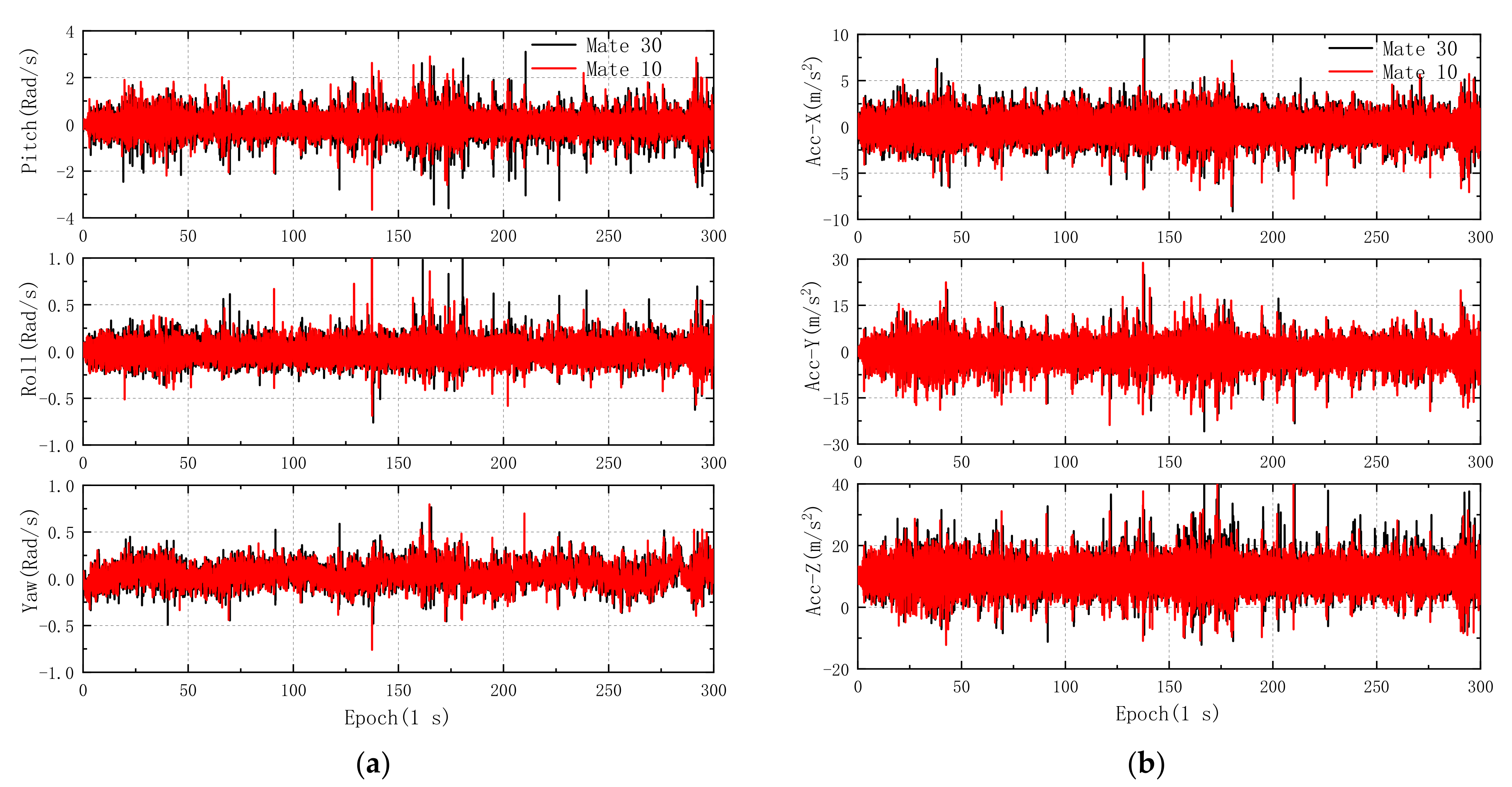
More than half of the carrier phase measurements cannot be observed in dynamic mode by the early single-frequency smartphones such as the Mate 10 in some areas where GNSS signal degrades slightly. Although the positioning accuracy of the Mate 10 is improved with the PPP/INS coupled model, its absolute positioning accuracy is still closely related to PPP accuracy. The weak positioning performance of single-frequency smartphones makes it difficult to meet the requirements of a precision location service, even in the open area.

(2)

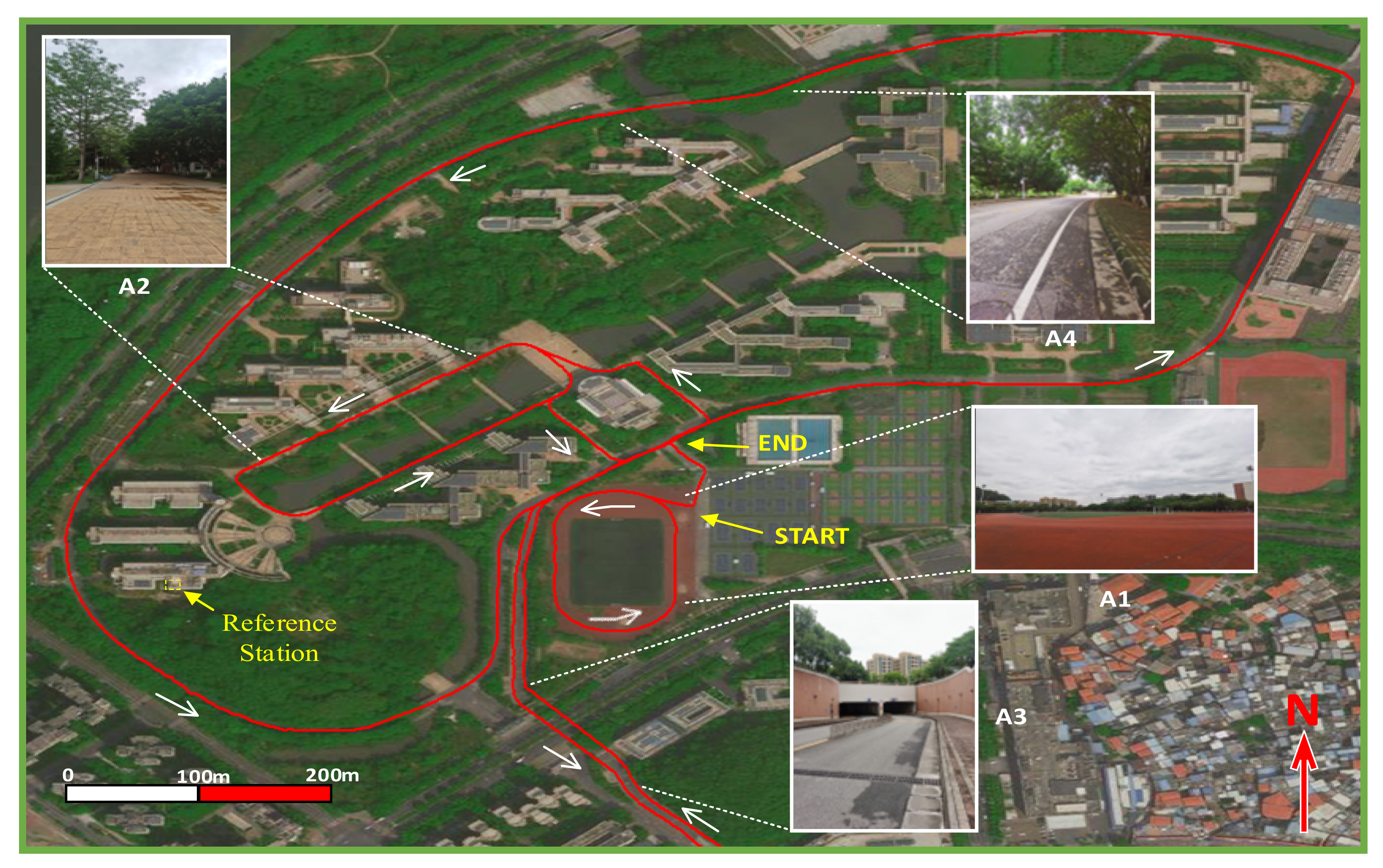
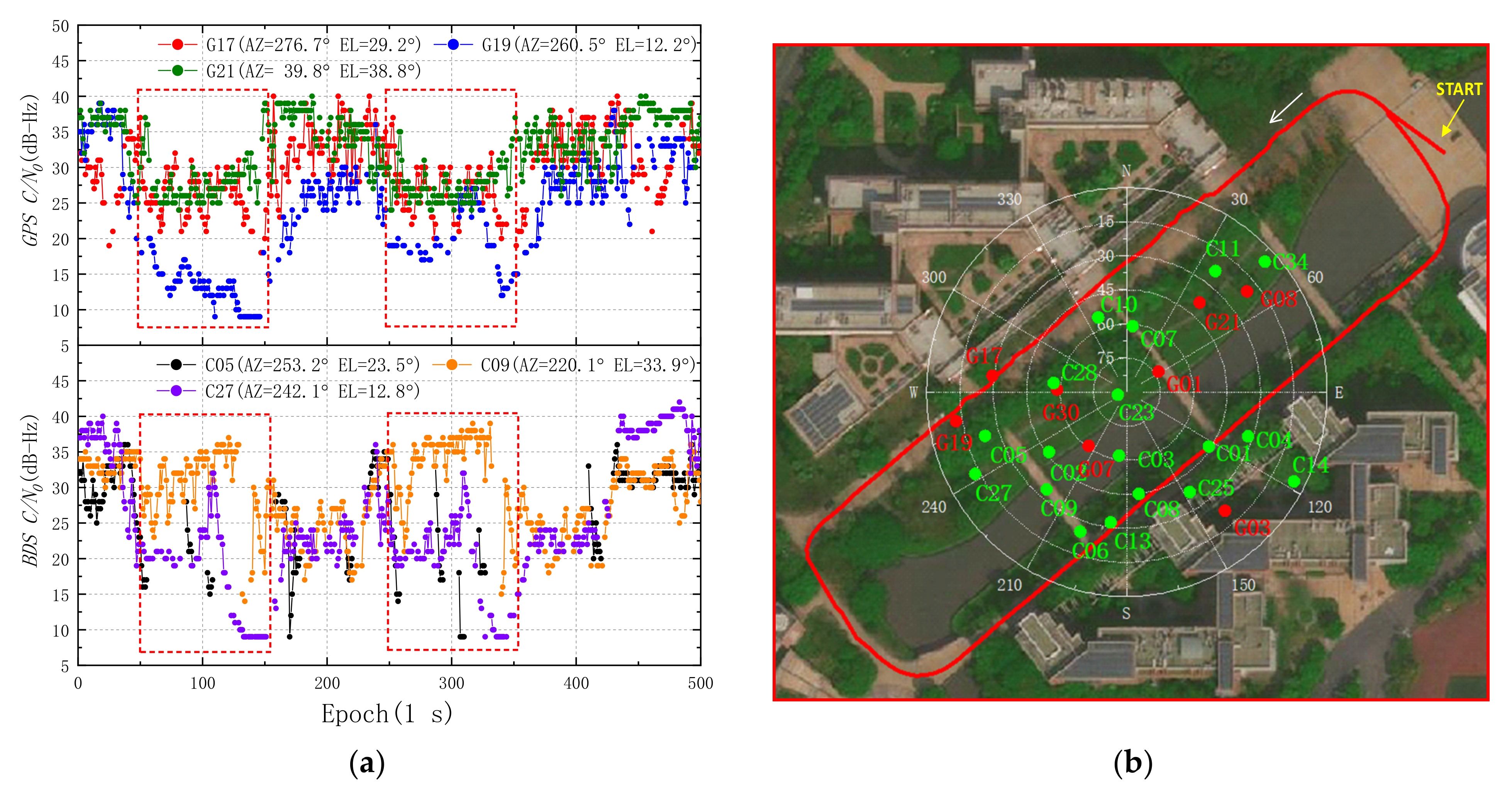
Unlike the geodetic receiver, the number of visible GNSS satellites observed by the Mate 30 fluctuate within a narrow range, which is caused by the weak multipath suppression ability of GNSS antenna of smartphones. In some areas where GNSS signals are significantly degraded due to the buildings and trees on both sides, the RMS of smartphone PPP horizontal positioning errors can even reach more than 10 m.

(3)

With the proposed PPP/INS coupled method, the RMS of PPP horizontal and vertical positioning errors on smartphone decreased significantly in various GNSS-degraded environments, and long trajectory experimental results indicated that the RMS of PPP/INS horizontal errors in the eastern and western areas decrease by 49.37% and 48.29%, respectively, compared with convention PPP solutions. Meanwhile, the results of several experiments also show that the positioning accuracy of PPP/INS is roughly equivalent to that of PPP/INS–ADIS.

(4)

Moreover, the position of smartphone can be outputted continuously while moving through the tunnel with a length of about 80 m; the PPP/INS trajectory deviation of smartphone in the tunnel remained stable. The horizontal deviation from the reference point is more than 8 m after 29 epochs, and the positioning points quickly approach the reference trajectory after leaving the tunnel.

In summary, the proposed PPP/INS coupled model integrated dual-frequency GNSS observations and IMU data from smartphones with C/N₀-dependent stochastic model and RKF model to improve the positioning performance in GNSS-degraded environments. However, the absolute positioning accuracy of GNSS PPP/INS in the open area is still closely related to PPP accuracy. Moreover, in the northern area of long trajectory experiments, the deviation of PPP/INS positioning gradually increases when the GNSS signals are blocked for a long time, which is related to the positioning error before entering the GNSS-signals-blocked area and the drift of INS. Therefore, we will further integrate other sensors such as cameras in smartphones for when the GNSS signals are blocked for long period of time, and conduct the experiments with multiple modes of transportation. In addition, with the improved performance of GNSS and internal IMU chipset of smartphones in the future, we can anticipate that high-precision position of smartphones will play a significant part in various navigation applications such as ITS and LBS.

References

1. Engelbrecht, J.; Booysen, M.J.; van Rooyen, G.J.; Bruwer, F.J. Survey of smartphone-based sensing in vehicles for intelligent transportation system applications. IET Intell. Transp. Syst. 2015, 9, 924–935. [Google Scholar] [CrossRef]
2. Specht, C.; Szot, T.; Dabrowski, P.; Specht, M. Testing GNSS receiver accuracy in Samsung Galaxy series mobile phones at a sports stadium. Meas. Sci. Technol. 2020, 31, 064006. [Google Scholar] [CrossRef]
3. Paziewski, J. Recent advances and perspectives for positioning and applications with smartphone GNSS observations. Meas. Sci. Technol. 2020, 31, 091001. [Google Scholar] [CrossRef]
4. Li, G.C.; Geng, J.H. Characteristics of raw multi-GNSS measurement error from Google Android smart devices. GPS Solut. 2019, 23, 90. [Google Scholar] [CrossRef]
5. Niu, X.J.; Zhang, Q.; Li, Y.; Cheng, Y.H.; Shi, C. Using Inertial Sensors of iPhone 4 for Car Navigation. In Proceedings of the IEEE/ION Position Location and Navigation Symposium (PLANS), Myrtle Beach, SC, USA, 23–26 April 2012; pp. 555–561. [Google Scholar]
6. Elarabi, T.; Suprem, A. Orientation and Displacement Detection for Smartphone Device Based Inertial Measurement Units. In Proceedings of the IEEE International Symposium on Signal Processing and Information Technology (ISSPIT), Abu Dhabi, United Arab Emirates, 7–10 December 2015; pp. 122–126. [Google Scholar]
7. Liu, W.K.; Shi, X.; Zhu, F.; Tao, X.L.; Wang, F.H. Quality analysis of multi-GNSS raw observations and a velocity-aided positioning approach based on smartphones. Adv. Space Res. 2019, 63, 2358–2377. [Google Scholar] [CrossRef]
8. Zhu, H.Y.; Xia, L.Y.; Wu, D.J.; Xia, J.C.; Li, Q.X. Study on Multi-GNSS Precise Point Positioning Performance with Adverse Effects of Satellite Signals on Android Smartphone. Sensors 2020, 20, 6447. [Google Scholar] [CrossRef]
9. Elmezayen, A.; El-Rabbany, A. Precise Point Positioning Using World’s First Dual-Frequency GPS/GALILEO Smartphone. Sensors 2019, 19, 2593. [Google Scholar] [CrossRef]
10. Wu, Q.; Sun, M.F.; Zhou, C.J.; Zhang, P. Precise Point Positioning Using Dual-Frequency GNSS Observations on Smartphone. Sensors 2019, 19, 2189. [Google Scholar] [CrossRef] [PubMed]
11. Chen, B.; Gao, C.F.; Liu, Y.S.; Sun, P.Y. Real-time Precise Point Positioning with a Xiaomi MI 8 Android Smartphone. Sensors 2019, 19, 2835. [Google Scholar] [CrossRef]
12. Zumberge, J.F.; Heflin, M.B.; Jefferson, D.C.; Watkins, M.M.; Webb, F.H. Precise point positioning for the efficient and robust analysis of GPS data from large networks. J. Geophys. Res. 1997, 102, 5005–5017. [Google Scholar] [CrossRef] [Green Version]
13. Heroux, P.; Kouba, J. GPS precise point positioning using IGS orbit products. Phys. Chem. Earth Part A-Solid Earth Geod. 2001, 26, 573–578. [Google Scholar] [CrossRef]
14. Linty, N.; Lo Presti, L.; Dovis, F.; Crosta, P. Performance analysis of duty-cycle power saving techniques in GNSS mass-market receivers. In Proceedings of the IEEE/ION Position, Location and Navigation Symposium (PLANS), Monterey, CA, USA, 5–8 May 2014; pp. 1096–1104. [Google Scholar]
15. Paziewski, J.; Sieradzki, R.; Baryla, R. Signal characterization and assessment of code GNSS positioning with low-power consumption smartphones. GPS Solut. 2019, 23, 98. [Google Scholar] [CrossRef]
16. Gogoi, N.; Minetto, A.; Linty, N.; Dovis, F. A Controlled-Environment Quality Assessment of Android GNSS Raw Measurements. Electronics 2019, 8, 5. [Google Scholar] [CrossRef]
17. Hakansson, M. Characterization of GNSS observations from a Nexus 9 Android tablet. GPS Solut. 2019, 23, 21. [Google Scholar] [CrossRef]
18. Humphreys, T.E.; Murrian, M.; van Diggelen, F.; Podshivalov, S.; Pesyna, K.M. On the Feasibility of cm-Accurate Positioning via a Smartphone’s Antenna and GNSS Chip. In Proceedings of the IEEE/ION Position, Location and Navigation Symposium (PLANS), Savannah, GA, USA, 11–14 April 2016; pp. 232–242. [Google Scholar]
19. Shinghal, G.; Bisnath, S. Conditioning and PPP processing of smartphone GNSS measurements in realistic environments. Satell. Navig. 2021, 2, 10. [Google Scholar] [CrossRef]
20. Gikas, V.; Perakis, H. Rigorous Performance Evaluation of Smartphone GNSS/IMU Sensors for ITS Applications. Sensors 2016, 16, 1240. [Google Scholar] [CrossRef] [PubMed]
21. Wang, L.; Li, Z.S.; Zhao, J.J.; Zhou, K.; Wang, Z.Y.; Yuan, H. Smart Device-Supported BDS/GNSS Real-Time Kinematic Positioning for Sub-Meter-Level Accuracy in Urban Location-Based Services. Sensors 2016, 16, 2201. [Google Scholar] [CrossRef] [PubMed]
22. Jukic, O.; Iliev, T.B.; Sikirica, N.; Lenac, K.; Spoljar, D.; Filjar, R. A method for GNSS positioning performance assessment for location-based services. In Proceedings of the 28th Telecommunications Forum (TELFOR), Belgrade, Serbia, 24–25 November 2020; pp. 89–92. [Google Scholar]
23. Yuan, Z.K.; Zhu, D.F.; Chi, C.; Tang, J.H.; Liao, C.Y.; Yang, X. Visual-Inertial State Estimation with Pre-integration Correction for Robust Mobile Augmented Reality. In Proceedings of the 27th ACM International Conference on Multimedia (MM), Nice, France, 21–25 October 2019; pp. 1410–1418. [Google Scholar]
24. Bahillo, A.; Aguilera, T.; Alvarez, F.J.; Perallos, A. WAY: Seamless Positioning Using a Smart Device. Wirel. Pers. Commun. 2017, 94, 2949–2967. [Google Scholar] [CrossRef]
25. Guo, L.; Wang, F.H.; Sang, J.Z.; Lin, X.H.; Gong, X.W.; Zhang, W.W. Characteristics Analysis of Raw Multi-GNSS Measurement from Xiaomi Mi 8 and Positioning Performance Improvement with L5/E5 Frequency in an Urban Environment. Remote Sens. 2020, 12, 744. [Google Scholar] [CrossRef]
26. Wang, L.; Li, Z.S.; Wang, N.B.; Wang, Z.Y. Real-time GNSS precise point positioning for low-cost smart devices. GPS Solut. 2021, 25, 69. [Google Scholar] [CrossRef]
27. Kaiser, S.; Wei, Y.Z.; Renaudin, V. Analysis of IMU and GNSS Data Provided by Xiaomi 8 Smartphone. In Proceedings of the 11th International Conference on Indoor Positioning and Indoor Navigation (IPIN), Univ Oberta Catalunya, Lloret de Mar, Spain, 29 November–2 December 2021. [Google Scholar]
28. Park, K.; Kim, W.; Seo, J. Effects of Initial Attitude Estimation Errors on Loosely Coupled Smartphone GPS/IMU Integration System. In Proceedings of the 20th International Conference on Control, Automation and Systems (ICCAS), Busan, Korea, 13–16 October 2020; pp. 800–803. [Google Scholar]
29. Yan, W.L.; Bastos, L.; Magalhaes, A. Performance Assessment of the Android Smartphone’s IMU in a GNSS/INS Coupled Navigation Model. IEEE Access 2019, 7, 171073–171083. [Google Scholar] [CrossRef]
30. Yan, W.L.; Zhang, Q.Z.; Wang, L.J.; Mao, Y.; Wang, A.S.; Zhao, C.S. A Modified Kalman Filter for Integrating the Different Rate Data of Gyros and Accelerometers Retrieved from Android Smartphones in the GNSS/IMU Coupled Navigation. Sensors 2020, 20, 5208. [Google Scholar] [CrossRef] [PubMed]
31. Chiang, K.W.; Le, D.T.; Duong, T.T.; Sun, R. The Performance Analysis of INS/GNSS/V-SLAM Integration Scheme Using Smartphone Sensors for Land Vehicle Navigation Applications in GNSS-Challenging Environments. Remote Sens. 2020, 12, 1732. [Google Scholar] [CrossRef]
32. Biswas, S.K.; Qiao, L.; Dempster, A.G. Effect of PDOP on performance of Kalman Filters for GNSS-based space vehicle position estimation. GPS Solut. 2017, 21, 1379–1387. [Google Scholar] [CrossRef]
33. Doong, S.H. A closed-form formula for GPS GDOP computation. GPS Solut. 2009, 13, 183–190. [Google Scholar] [CrossRef]
34. Kouba, J.; Springer, T. New IGS Station and Satellite Clock Combination. GPS Solut. 2001, 4, 31–36. [Google Scholar] [CrossRef]
35. Brunner, F.K.; Hartinger, H.; Troyer, L. GPS signal diffraction modelling: The stochastic SIGMA-Delta model. J. Geod. 1999, 73, 259–267. [Google Scholar] [CrossRef]
36. Hartinger, H.; Brunner, F.N. Variances of GPS Phase Observations: The SIGMA-e Model. GPS Solut. 1999, 2, 35–43. [Google Scholar] [CrossRef]
37. Gu, S.F.; Dai, C.Q.; Fang, W.T.; Zheng, F.; Wang, Y.T.; Zhang, Q.; Lou, Y.D.; Niu, X.J. Multi-GNSS PPP/INS tightly coupled integration with atmospheric augmentation and its application in urban vehicle navigation. J. Geod. 2021, 95, 64. [Google Scholar] [CrossRef]
38. Du, Z.Q.; Chai, H.Z.; Xiao, G.R.; Yin, X.; Wang, M.; Xiang, M.Z. Analyzing the contributions of multi-GNSS and INS to the PPP-AR outage re-fixing. GPS Solut. 2021, 25, 81. [Google Scholar] [CrossRef]
39. Yang, Y.; He, H.; Xu, G. Adaptively robust filtering for kinematic geodetic positioning. J. Geod. 2001, 75, 109–116. [Google Scholar] [CrossRef]
40. Guo, F.; Zhang, X.H. Adaptive robust Kalman filtering for precise point positioning. Meas. Sci. Technol. 2014, 25, 105011. [Google Scholar] [CrossRef]
41. Yang, Y.; Song, L.; Xu, T. Robust estimator for correlated observations based on bifactor equivalent weights. J. Geod. 2002, 76, 353–358. [Google Scholar] [CrossRef]
42. Zhang, Q.Q.; Zhao, L.D.; Zhao, L.; Zhou, J.H. An Improved Robust Adaptive Kalman Filter for GNSS Precise Point Positioning. IEEE Sens. J. 2018, 18, 4176–4186. [Google Scholar] [CrossRef]
43. Saastamoinen, J. Contributions to the theory of atmospheric refraction. II. Refraction corrections in satellite geodesy. Bull. Géodés. 1972, 105, 279–298. [Google Scholar] [CrossRef]
Figure 1. View of the experiment devices. Left: Huawei Mate 10, triaxial inertial sensor ADIS16405, Huawei Mate 30, and South geodetic receiver. Right: the reference station is placed in the open area on the roof.
Remotesensing 14 04469 g001
Figure 2. Dynamic trajectories of the whole experiments. The pictures named A1, A2, A3, and A4 show some realistic GNSS-degraded environments for each experiment, and the yellow box shows the location of the reference station. A denotes the area.
Remotesensing 14 04469 g002
Figure 3. Number of GNSS satellites and PDOP values on the playground in area 1. (a) GPS and BDS measurements observed by Mate 30; (b) GPS measurements observed by the geodetic receiver and Mate 10.
Remotesensing 14 04469 g003
Figure 4. Carrier-to-noise power density ratio values of GNSS satellites observed by the Huawei Mate 30 on the playground. (a) Some GPS and BDS satellites whose signals are degraded due to the trees, and the red box shows the C/N0 value in the area marked by the yellow box in Figure 4b. (b) Left: reference trajectory and sky plot of GPS and BDS. Right: realistic environment marked by the yellow box.
Remotesensing 14 04469 g004
Figure 5. Number of GNSS satellites and PDOP values on the sidewalk in area 2. (a) GPS and BDS measurements observed by Mate 30; (b) GPS measurements observed by the geodetic receiver and Mate 10.
Remotesensing 14 04469 g005
Figure 6. The C/N0 values of GNSS satellites observed by the Huawei Mate 30 on the sidewalk in area 2. (a) The same GPS and BDS satellites as in Figure 4a, and the red box shows the C/N0 values of the satellites decrease significantly. (b) Reference trajectory and sky plot of GPS and BDS.
Remotesensing 14 04469 g006
Figure 7. Comparisons of the IMU data from Mate 30 and ADIS16405. (a) Three-axis gyroscope; (b) three-axis accelerometer.
Remotesensing 14 04469 g007
Figure 8. Comparisons of the IMU data from Mate 30 and Mate 10. (a) Three-axis gyroscope; (b) three-axis accelerometer.
Remotesensing 14 04469 g008
Figure 9. Comparison of cumulative distribution function (CDF) of three-axis gyroscope and accelerometer differences from Mate 30, ADIS16405, and Mate 10. (a) Three-axis gyroscope; (b) three-axis accelerometer. Mate 30–ADIS16405 denotes the CDF of gyroscope and accelerometer differences between Mate 30 and ADIS16405, and Mate 30–Mate 10 denotes the CDF of gyroscope and accelerometer differences between Mate 30 and Mate 10.
Remotesensing 14 04469 g009
Figure 10. The flow chart of GNSS PPP/INS integrated navigation on smartphones.
Remotesensing 14 04469 g010
Figure 11. GPS PPP and PPP/INS solutions from Huawei Mate 10 on the playground. (a) Trajectories of GPS PPP and PPP/INS solutions. (b) Comparison of GPS PPP and PPP/INS solutions with reference points. The E and N denote east and north direction, respectively.
Remotesensing 14 04469 g011
Figure 12. GPS PPP and PPP/INS solutions from Huawei Mate 30 on the playground. (a) Trajectories of GPS PPP and PPP/INS solutions. (b) Comparison of GPS PPP and PPP/INS solutions with reference points.
Remotesensing 14 04469 g012
Figure 13. GPS/BDS PPP and PPP/INS solutions from Huawei Mate 30 on the playground. (a) Trajectories of GPS/BDS PPP and PPP/INS solutions. (b) Comparison of GPS/BDS PPP and PPP/INS solutions with reference points.
Remotesensing 14 04469 g013
Figure 14. GPS/BDS PPP and PPP/INS solutions from Huawei Mate 30 on the sidewalk. (a) Trajectories of GPS/BDS PPP and PPP/INS solutions. (b) Comparison of GPS/BDS PPP, PPP/INS, and PPP/INS–ADIS solutions with reference points. PPP/INS–ADIS denotes that the data of ADIS16405 were used in the PPP/INS coupled model instead of the IMU data of smartphone.
Remotesensing 14 04469 g014
Figure 15. GPS/BDS PPP and PPP/INS solutions from Huawei Mate 30 in the tunnel. (a) Left: trajectories of GPS/BDS PPP and PPP/INS solutions. Right: the realistic environment marked in the red box. (b) Comparison of GPS/BDS PPP and PPP/INS solutions with reference points, and the red box shows the GPS/BDS PPP/INS solutions in the tunnel.
Remotesensing 14 04469 g015
Figure 16. The long trajectories of GPS/BDS PPP, PPP/INS, and PPP/INS–ADIS solutions using Huawei Mate 30 and ADIS16405. Left: the realistic environment marked in the purple box 3. Right: the realistic environment marked in the purple box 1. The areas where the number of satellites cannot meet the requirements of GNSS positioning are marked by red boxes 2 and 4.
Remotesensing 14 04469 g016
Figure 17. Comparison of Huawei Mate 30 GPS/BDS PPP, PPP/INS, and PPP/INS–ADIS solutions with reference points. The boxes 1, 2, 3, and 4 corresponds to the boxes in Figure 16.
Remotesensing 14 04469 g017