Abstract
The article discusses an important issue of railway line construction and maintenance, which fundamentally is the verification of geometric parameters of the railway track. For this purpose, mobile measurements have been performed using a measuring platform with two properly arranged GNSS receivers, which made it possible to determine the base vector of the platform. The measuring functionality of the system was extended by IMU. In this article, the effect of measuring conditions on the accuracy of the results collected from GNSS receivers is analyzed. In particular, the advisability of digital filtering of the recorded coordinates to eliminate disturbances is indicated. The article also presents the possible use of GNSS devices and the IMU unit for determining the direction angle and the longitudinal and lateral inclination angles of the railway track. This makes it possible to verify the track geometry in the horizontal plane by determining the positions of straight sections, circular arcs, and transition curves. It is indicated that the results of measurements are repeatable despite the dynamic interaction between the railway track and the measuring platform. The results confirm the usefulness of the applied GNSS and IMU signal processing method for monitoring the geometrical parameters of the railway track in operating conditions.
1. Introduction
In order to detect changes or analyze trends in individual parameters, the monitoring of the technical condition used is aimed at planning regulatory processes or even preventing potential failures.
In the monitoring of the rail transport infrastructure, one can distinguish the evolution from manual maintenance, through methods related to the use of many sensors of various physical quantities, to solutions such as for Industry 4.0 [1], for which improved methods of interpretation of data from related monitoring are required, e.g., sensor fusion, big data analytics, or digital twins [2,3,4,5,6].
During the railway track operation, its shape is subject to horizontal and vertical deformations, which means that monitoring of its technical condition is required. This is completed by performing relevant measurements to determine the railway track axis and compare it with the designed shape. For this purpose, a precise geodetic inspection of a railway line is carried out, both in the construction and operation stages. The railway track measurements can be divided into four main categories.
The first category includes static chord techniques which make it possible to measure the sagitta being the measure of railway geometrical irregularities [7,8]. Here, traditional railway surveying methods are used and are more frequently combined with GNSS (Global Navigation Satellite System) techniques, all performed in a stationary mode of measurement. This group also includes measuring trolleys [9,10,11,12,13]. These solutions allow for obtaining measurement results of local nature and also of global relevance when coupled with the GNSS. The common features of the methods composing this group are high accuracy measurement and small speed of motion of the measuring system (typically from 0.1 to about 1 km/h). The main aim of the performed solutions is to evaluate the irregularities of railway tracks and to check the position that consists of the real track axis with the designed one.
The second group of methods includes automatic measurement systems. The measuring devices are installed on special diagnostic trolleys or vehicles. Chord techniques are also used in this group, as well as satellite location systems or inertial measurement units. The systems in this group are characterized by slightly higher measuring speeds—typically from 3 to 5 km/h [14,15,16,17].
The third group comprises all types of inspection vehicles used for diagnostics of railway track geometry and technical condition of elements of railway track surface and substructure. As a rule, these vehicles move at higher speeds, from about 50–60 km/h to even as much as 250 km/h [18,19]. Their measuring performance is excellent, but high measurement accuracy is only obtained when the rail irregularities are evaluated. Converting the rail geometrical irregularities evaluated based on the measured sagitta–to–chord ratio to its shape description in the X, Y, H space, where X and Y are the coordinates in the horizontal plane and H is the height related to Normaal Amsterdams Peil (NAP), is a complex problem. The global parameters are only used for the spatial positioning of the rail to evaluate its irregularity [20].
A remarkable change, in both qualitative and quantitative senses, has been brought about by methods making use of GNSS, and Permanent GNSS Networks [6,10,15,21,22]. By introducing corrections to the earlier recorded coordinates in the so-called post-processing, these methods offer a very efficient and accurate measurement of railway track coordinates. In the InnoSatTrack project, a method is proposed which makes use of several GNSS receivers in mobile arrangement, complemented by an IMU and MLS (Mobile Laser Scanning). This method allows railway track axis measurements with a tolerance of 1 cm at the measuring speed level of 30 km/h [22].
The above method also allows to make use of additional measured quantities, such as lateral and longitudinal inclination angles and direction angle of the track. The information on inclination angles in horizontal and vertical planes is required when introducing corrections to the railway track axis coordinates, which is related to the fact that the GNSS receivers are installed above the plane determined by the rail heads [22,23]. The quality of the performed measurement of coordinates can also be evaluated based, for instance, on the estimated base vector and reference distances between the receivers [22,24].
The novel aspects discussed in the article include:
- analyzing the effect of measurement conditions observed on the railway line on the accuracy of position measurement obtained from GNSS receivers, and possible further detection of disturbed coordinate values recorded in mobile measurements,
- demonstrating the repeatability of the high-precision measurement data obtained from multiple passages of the measuring platform along the same track segment,
- proposing a better utilization scheme of coordinates obtained based on GNSS when the IMU system cannot be installed by applying smoothing digital filtering to eliminate disturbances introduced, for instance, by natural obstacles,
- determining the railway track curvature based on Savitzky–Golay algorithm,
- proposing the fusion of GNSS signals, the track’s longitudinal and lateral inclination angles and direction angle recorded by the IMU, the base vector length, and the track curvature for developing geometry segmentation algorithms.
- The basic aims of the work include:
- performing mobile measurements with systems, GNSS and IMU/INS, and the use of advanced measurement and signal post-processing methods with digital filtering on the example of the railway line section of characteristic geometry and natural obstacles,
- determining the usability range of GNSS signals at the occurrence of short-term disturbances. In this case, the GNSS signal quality index and the length of the measuring system base vector were used for detecting qualitatively incorrect coordinate records,
- demonstrating the repeatability of measurements of longitudinal and lateral inclination angles and the direction angle of the railway track in mobile measurement conditions, and their accuracy by comparing with the data given in the documentation,
- proposing and verifying the method’s applicability concerning the measurement of longitudinal and lateral inclination angles and direction angles of the railway track, with simultaneous indication of the requirement concerning the accuracy of measurement,
- indicating possible applications of mobile GNSS and IMU measurements for developing efficient algorithms for the automatic reconstruction of railway track geometry in both horizontal and vertical planes, which includes identifying constant inclination sections, grade–line alignment arcs, as well as straight sections, circular arcs, and transition curves.
Section 2 presents experimental studies performed on the selected railway line section with complex geometry, while Section 3 describes a novel approach that makes use of digital filtering when post-processing the results obtained from GNSS receivers. Attention was paid to the selection of filtering parameters, which was completed using the Whittaker and Savitzky–Golay algorithms. Section 4 discusses the measurements performed with IMU/INS, in particular the issue of high-precision recording of longitudinal and lateral inclination angles and direction angles of the railway track. Identifying the elements of railway track geometry is presented in Section 5, using the studied railway line as an example. The results of the performed measurements and calculations are presented in graphical form. Section 6 summarizes the work and presents conclusions, indicating the possible potential for the development of algorithms performing automatic reconstruction of railway line geometry to support railway infrastructure management processes.
2. Experimental Studies on the Railway Line
The railway lines have a precisely defined track macro–geometry. In the horizontal plane, their geometry is comprised of straight sections, circular arcs, and transition curves, while in the vertical plane, constant inclination sections and grade–line alignment arcs can be named. At the same time, the parameter of railway track cross-section is cant. The railway track geometry determines the permissible speed of trains on a given line section. As a result of constructional and maintenance shortcomings, some deformations appear with respect to the designed track geometry in the global reference system. This process of track geometry degradation grows with time and is observed as micro-geometrical deviations, the so-called horizontal and vertical imperfections [25,26,27,28]. It is noteworthy that large-scale track geometry deformations in relation to the designed shape, and cases of irregularity of relatively short wavelength are analyzed separately. Therefore, getting an overall view of the railway track geometry requires measurements ranging from several millimeters up to a dozen of kilometers or more, depending on whether the analysis concerns the railway track microgeometry or global coordinates of its trajectory. To precisely determine the lateral and longitudinal inclination of the railway track, high-resolution angle measurements are also required, at least to the order of hundredths of a degree.
The experimental studies were completed in Poland on a single–track PKP (Polish State Railway) railway line no. 211, on the Kościerzyna–Lipusz section between km 68 + 500 and km 65 + 700 (Figure 1). The basic measurements were made on the railway line fragment consisting of four straight sections, three circular arcs (curves), and a relevant number of transition curves linking the straight sections with the arcs. The railway line trajectory and the measuring area are shown in Figure 1.
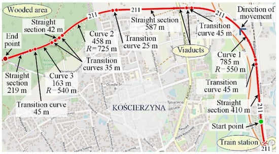
Figure 1.
The trajectory of railway line no. 211 from Kościerzyna train station https://www.openrailwaymap.org (accessed on 9 December 2021).
In its initial part from the start point of mobile measurements, the railway line passes the area without large natural obstacles for GNSS signal reception, but after Curve 1, two road viaducts disturb the reception of the GNSS signal. Then, the line passes an open area until Curve 2, after which it enters the woodland. These varying area conditions, illustrated in Figure 2, are of high significance for GNSS signal reception and, consequently, for the accuracy of railway track coordinate measurement.
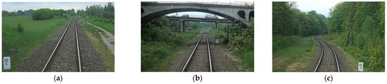
Figure 2.
Views of sections of railway line no. 211: (a) open area along initial section; (b) viaducts in central section; (c) final woodland section.
To measure the shape of the selected railway line section, two high-precision GNSS Leica GS18 receivers, marked A and B, and the Ekinox2-U IMU unit were mounted on the measuring platform. The measuring instruments were installed on a typical PKP service vehicle, i.e., a PWM15 trailer with a wheel axis distance equal to 6.39 m, pulled by a WM15 motor car. This train arrangement is shown in Figure 3. The receivers, A and B, mounted at the reference distance, lAB = 5.9 m, along the longitudinal axis of the platform, determine the so-called measuring base vector. The IMU unit, placed in the symmetry point of lAB and as well as the symmetry of the trailer, cooperated with two additional Aero AT1675-382 GNSS antennas, creating, with the computing unit, the so-called INS system. The IMU unit recorded the lateral inclination angle (roll), the longitudinal inclination angle (pitch), and the direction angle (yaw). The antennas of the INS unit made it possible to record the position coordinates of this device. The accuracy of INS, defined as RMSE of 2D position in post-processed data using Inertial Explorer with at least Precise Point Positioning data, is equal to 3 cm in case of GNSS signal lost for less than 10 s. At Real-Time Kinematics (RTK) a typical accuracy position goes to 1 cm.
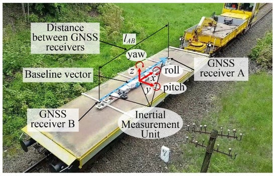
Figure 3.
The measuring platform with GNSS and IMU units’ placement, where: yaw, roll, and pitch represent, respectively, the direction, and lateral and longitudinal inclination angles of the track.
On the selected railway line segment, a number of measuring platform passages were executed with different speeds and different operation modes of the measuring instruments. Selected passage parameters are shown in Figure 4a, while the recorded railway track coordinates are presented in Figure 4b in the coordinate system PL-2000 (the Y-axis is directed from West to East, and the X-axis is from South to North). PL-2000 is the system of plane coordinates that is presently in force in Poland. It was developed as a result of Gauss–Krüger mapping of the ellipsoid GRS 80 (Geodetic Reference System 1980) with longitudes 15°E, 18°E, 21°E, and 24°E [22].
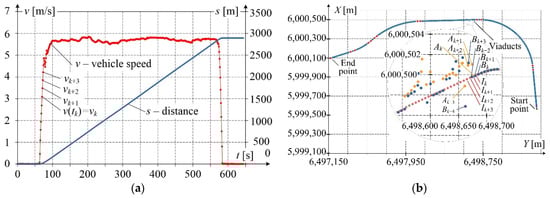
Figure 4.
Results of measurement recorded in RTN mode: (a) speed changes and covered distance; (b) trajectory of railway line coordinates in PL-2000 reference system—where Ak, Bk, and Ik are the coordinates recorded respectively by the receiver’s A, B, and INS at moments tk, tk+1, … with period 1 s, in the enlarged scale is shown a disturbance related to the passage under the road viaducts.
During the measurement, the coordinates were recorded in RTN (Real Time Network) mode, while the corrections obtained from ground reference stations to improve their accuracy were introduced in real-time every 1 s. In Figure 4a one can observe the measuring platform speed vk, recorded every 1 s, (the average speed was approximately equal to 20 km/h ≈ 5.5 m/s), and the calculated distance s covered by the platform. This distance amounted to slightly less than 3 km in total. Additionally, in the railway line trajectory (Figure 4b), the starting and final points of the measurement are marked, and the points at which the section type changes between straight section, circular arc, and transition curve. The magnified trajectory fragment, corresponding to the vicinity of road viaducts, presents the coordinates recorded by receivers Ak and Bk and by INS – Ik working in RTN mode, every 1 s. Even a preliminary qualitative visual analysis makes it possible to notice the presence of significant deviations from the railway track axis, which is the effect of obstructing the GNSS receiver by the viaducts. The recorded Ik values correspond approximately to the track axis. For longer times of GNSS signal decay, the error of Ik increases.
The error of coordinate determination from the GNSS signal is affected, among other factors, by the number of available satellites. To estimate this error, the quality index CQ3D (Coordinate Quality in 3D space) was recorded, and the length of the base vector was calculated. Figure 5 presents changes in the relative number of available satellites n/nmax, where nmax = 16. What is clearly visible is the reduced number of available satellites in the vicinity of viaducts and in the woodland area. The quality index CQ3D reaches visibly higher values in the vicinity of viaducts and in the woodland area than in the open area. A high value of CQ3D means a larger measurement error. The base vector length lAB, calculated from the coordinates recorded by receivers A and B and related to the real reference length lref measured with high accuracy using an independent method during platform stop, also confirms the occurrence of unacceptable results recorded in the vicinity of viaducts, and less accurate results in the woodland area, as compared to those recorded in the open area.
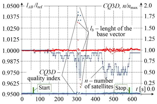
Figure 5.
Variability of the relative length of measuring base vector, number of available satellites, and quality index.
The base vector length lAB at time tk is given by the formula:
where YA(tk) and XA(tk), and YB(tk) and XB(tk) are plane coordinates recorded by receivers A and B.
Formula (1) omits the vertical coordinate, as the effect of a longitudinal inclination of the railway track on the base vector length is negligibly small.
The application of GNSS receivers working with a frequency of 20 Hz, or even 100 Hz, in combination with data post-processing provides opportunities for obtaining high measuring density, e.g., every 0.5 m, at the platform speed of 10 m/s and sampling frequency of 20 Hz. Simultaneously, small measurement errors are achieved, as they are reduced by corrections introduced in post-processing. Figure 6 shows the measurement results obtained in post-processing, for the operating frequency of the antennas equal to 20 Hz. Compared to Figure 4b, a much better quality of the GNSS results can be observed. In particular, their density is higher than that of 1-s INS records, which facilitates further processing to determine the railway track geometry. The analysis of the results of the GNSS coordinates recorded in the RTN mode with a frequency of 1 Hz shows that passing of the measuring platform under the road viaducts results in two periods of disturbances of the signals recorded by receivers A and B. These periods last for about 8 s each, with an approximately 4-s period of correct recording between them (see the magnified fragment in Figure 4b). A more detailed disturbance analysis can be made in post-processing for the data recorded with a frequency of 20 Hz. As shown in Figure 6, the processed results recorded by receiver A and the INS device reveal clear disturbances introduced by the viaducts. For the measuring platform speed of 20 km/h, the distance covered by the platform during the time of occurrence of these disturbances is about 45 m.
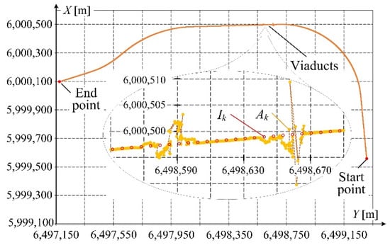
Figure 6.
Results of post-processing of the signal from receiver A in 20 Hz mode and from INS – Ik markers in 1 Hz mode.
3. Processing of Measurement Results Obtained from GNSS Receivers
Natural obstacles introduce disturbances to the GNSS signals recorded in mobile measurements. The disturbed points can be distant from the real track trajectory by several meters or more, and could even be totally lost. Such cases of an erroneous recording should be identified at the stage of measuring signal analysis. For this purpose, the values of the quality index CQ3D can be used along with the number of available satellites. Alternatively, it can be completed by controlling the base vector length lAB(tk). A clear correlation has been established between these quantities, as shown in Figure 5, which provides opportunities for using algorithms characteristic for data fusion to ensure a high value of the identification confidence index. Correct identification of erroneous measurement results enables their elimination from the data set, with simultaneous signalization of the appearance of a gap in the data stream. Another approach is based on digital filtering making use, for instance, of the well-known Whittaker algorithm [24,29,30]. Significant advantages of this algorithm include correct operation of the filter even when a substantial amount of data is missing, which is achieved by introducing the vector P with weight factors, e.g., equal to 0 or 1 to select the measurement data. In this case, high computing speed can be achieved due to the use of sparse matrices and controlling the operation with only one parameter λ.
For the data series ξi with length N, where i = 1, 2, …, N, and equal spaces (with respect to time or distance), the filtering algorithm finds continuous series σi which match ξi. To do this, a compromise is to be found between two contradictory goals: fidelity of matching and roughness.
The measure of mismatch between σi and data series ξi can be calculated as the sum of squares of differences:
At the same time, a simple and effective measure of roughness is calculating the sum of second-order squares of differences:
Combining these two goals gives the sum Q = S + λR, where the parameter λ should be selected such as to obtain a relevant balance between roughness and fidelity of matching.
The idea of the least squares method with penalty function is to find the value of σi which minimizes Q. The algorithm modified for a case when some data in the input signal are missing can be formulated as:
where P is a matrix with weight factors pi values on the diagonal.
In the reported case, the input data ξi to the Whittaker algorithm contains the measured coordinates Y(ti) = Yi, X(ti) = Xi, for i = 1, 2, 3, …, where ti+1 – ti = T is a constant value defining the sampling time of the measurement, and P is the weight vector with data correctness indices pi, elaborated based on the analysis of coefficients of the quality index CQ3D and the base vector length lAB. The parameter λ was found through optimization.
Figure 7 shows the effect of filtering the Y and X coordinates recorded by receivers A and B in RTN mode every 1 s. The reference signal in this case was the trajectory measured using the INS system. The application of filtering eliminated signal discontinuities and decreased the distance between the reference trajectory and the one recorded by the receivers. Since the sampling frequency was relatively low and the majority of the disturbed measuring points A and B were situated on one side with respect to the reference axis, the trajectories AFilter 1 and AFilter 2 after filtering still deviated from the expected values, despite attempts to optimize the parameters of the Whittaker algorithm (AFilter 1 corresponds λ = 2 while AFilter 2 λ = 90). This indicates some limitations of GNSS signal recording in RTN mode to identify the railway track geometry. Figure 7b shows the same fragment of the track axis trajectory but drawn based on GNSS signals recorded with a sampling frequency equal to 20 Hz and corrected in post-processing. Here, a different distribution of points recorded by receiver A when the measuring platform passed the viaducts with respect to the reference INS curve is observed. As for the RTN signal, the 20 Hz coordinates were filtered using the Whittaker algorithm with the same λ parameter. The obtained trajectory AFilter differs only slightly from the reference INS curve. This demonstrates the possibility to use the GNSS signal also when disturbances occur on relatively long stretches of track. These cases, however, require a proper selection of measurement and filtering parameters.
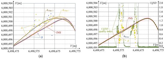
Figure 7.
Results of filtering: (a) the trajectories AFilter 1 and AFilter 2 obtained by the Whittaker algorithm with the coordinates of the receivers A and B and INS (details see in Figure 4) in RTN mode every 1 s; (b) the trajectory AFilter after post-processing of signal recorded with 20 Hz frequency by receiver A, against the 1–s INS results, additionally, the quality indicator CQ3D is marked.
When identifying the geometry of the railway track axis in the horizontal plane, an essential parameter is the direction angle of the track, i.e., the horizontal angle of the track in the geodetic coordinate system. Figure 8a shows the direction angle αGNSS of the railway track, analytically determined from the GNSS signal after post-processing. For comparison, the figure also presents the angle α measured by the INS system and the difference Δα between these two signals. For a high–quality GNSS signal, the difference Δα does not exceed 0.2 degrees, which is a very good result when taking into account the range of the measured quantities. The appearance of a disturbance during the platform passage under the viaducts affects the direction angle similar to the horizontal Y and X coordinates. The values of the direction angle can also be filtered, as shown in Figure 8b. After applying various filter parameters, the difference Δα with respect to the reference value was reduced to a level not exceeding 1.2 degrees. This is a satisfying result, in particular when the disturbances appear on the track section with constant or linearly changing direction angle, which corresponds, respectively, to the straight section or circular arc of the track. What is noteworthy here, the railway line design and construction principles say that the track axis geometry cannot change abruptly and in a discrete manner, which is a significant prerequisite when developing an algorithm for its identification.
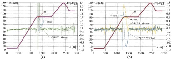
Figure 8.
Results of direction angle measurement: (a) αGNSS—from GNSS and α—from INS, with angle difference Δα = α – αGNSS; (b) from GNSS after Whittaker filtering αFilter 1 and αFilter 2 and from INS α, with angle differences Δα1 = α – αFilter 1 and Δα2 = α – αFilter 2.
The issue of track axis geometry identification is related to the track surface plane defined by the top points of rail sequences. By default, the GNSS antennas are situated above this plane, which imposes the need to correct the recorded coordinates, especially in the presence of track cant [22]. To determine these corrections, one should know the value of the lateral inclination angle αt at the measurement point. The longitudinal inclination angle αv affects the position of GNSS antennas much less. These corrections cannot be determined from GNSS signals, and an additional measuring instrument, IMU/INS, in this case, should be used. The information on the course of changes of angles αt and αv can additionally be used as input parameters to the algorithm identifying the track axis geometry in both horizontal and vertical planes.
4. Processing Results of IMU Measurement
The inertial measurement units (IMU) extended to the INS system allow recording with high precision lateral and longitudinal inclination angles and the direction angle of the railway track. Moreover, they extend the functional recording of coordinates when the GNSS signal is lost. The sampling times of GNSS signals and IMU sensors are different. For GNSS, the sampling frequency is usually between several and several tens of samples per second, while for IMU it is of the order of hundreds. In the presented results of measurements, the GNSS receiver worked with 20 Hz frequency, the INS antenna with 5 Hz, and IMU with 100 Hz. The IMU resolution of the angle measurement was 0.05°. Figure 9, Figure 10 and Figure 11 present the results recorded during eight measuring passages of the same track section.
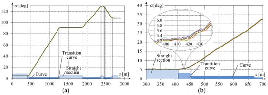
Figure 9.
Railway track direction angle obtained from multiple passages: (a) entire curve; (b) fragment in an expanded scale.
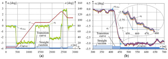
Figure 10.
Direction and lateral inclination angle of the track: (a) direction angle α from INS, and lateral inclination angles: αt from measurement and αt Doc from documentation, with indicated types of railway track sections; (b) in expanded scale from multiple passages.
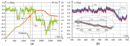
Figure 11.
Height and longitudinal inclination angle of the track: (a) relative track position height changes: ΔhINS from INS and ΔhA from GNSS receiver A, and longitudinal inclination angles: αv from measurement and αv Doc from documentation; (b) in expanded scale from multiple passages.
Figure 9 shows changes in the railway track direction angle, with an additional indication of straight sections, circular arcs, and transition curves taken from the railway line documentation. The obtained results reveal high repeatability, with an error below ±0.1°.
Figure 10 presents the direction angle α and the lateral inclination angle αt of the track as a function of the covered distance. The included lateral inclination angle αt Doc taken from the railway line documentation indicates straight sections, transition curves, and circular arcs.
Likewise, Figure 11 presents the longitudinal inclination angle αv obtained from the measurement and αv Doc from the documentation. Additionally, track position height changes ΔhINS from INS and ΔhA from GNSS receiver A are included. Height disturbances corresponding to the times of measuring platform passage under the viaducts can be clearly observed in the ΔhA curve.
The results recorded during multiple passages testify to the high precision of measurement, even for periods of small longitudinal railway track inclination. The convergence of measurement results with data from the documentation is also clearly visible.
5. Identifying the Railway Track Geometry
The railway track geometry is decisive for train running parameters. The task of determining railway line coordinates is executed using various measuring techniques [20,21,24,31,32,33]. In this task, the key issue is to identify particular track geometry elements: straight sections, circular arcs, and transition curves [14,21,31,33,34,35,36,37,38,39]. For this purpose, the distribution of track axis curvature along the examined track segment can be used. In [2] an odometric algorithm based on the equations of motion of a body moving along the track was used. A multi-sensor measurement system was used, inter alia, for linear and angular velocity. In [32,38] complex iterative algorithms are used concerning the determination of the directional angles of the track from the registration of GNSS coordinates, which are then used to approximate the curvature of the track. As in [36], the chord method is used. In both cases, measurement results proved to be sensitive to movement disorders.
The new aspects discussed, among others, in this article are to indicate the required INS parameters, in particular in terms of measuring angles and the use of efficient filtering and derivatives approximation algorithms of measurement results, taking into account the quality indicator of this data.
In analytical considerations concerning railway track axis design, the measure of track curvature on nonlinear sections is the curvature given by the formula:
where Δφ is the angle between tangents to the curve at the endpoints of the arc, and Δs is the arc length.
For a parametrically described curve x(t), y(t), its curvature at a given point is:
where t is the parameter, and x′(t), x″(t), y′(t), y″(t) are, respectively, the first and second-order derivatives.
The radius of the curve at a given point is defined as the inverse of the absolute value of its curvature at this point:
Determining the railway track curvature κ from definition (5) or Formula (6), when based on the measured coordinates, is difficult due to its discrete form. An additional inconvenience is some uncertainty of measurement data related to the class of the used measuring instruments and characteristics of the applied measurement method. Another possible source of uncertainty is related to disturbances of the measured trajectory resulting from the motion of the measuring platform on the track. All this makes it advisable to perform digital data processing which will give approximate values of curvature. However, this approach is extremely complex in systems of directly linked curves—without straight sections separating them. Segmenting a system that consists of several (sometimes even more than ten) curves based on the approximation of measurement data in the coordinate system PL-2000 is a time-consuming computation process that optimizes the matching error. Moreover, in some configurations, one can expect many solutions close to each other in matching the quality and simultaneously different with respect to the obtained parameters (number, type, and length of curves, as well as boundary curves).
It is noteworthy that using Formula (5) in a discrete data analysis may lead to significant local changes of values in curvature computations. The possibility to make use of the parametric relation (6) results from the fact that the measured railway track axis coordinates are expressed, as a function of time, in the plane coordinate system PL-2000. However, in this case, the first and second derivatives of coordinates Y(t) and X(t) should be calculated numerically, which, bearing in mind the abovementioned features of the processed measurements, is a complex issue. In the present study, the derivatives were calculated using the well-known Savitzky–Golay algorithm, and filtering was performed using the Whittaker algorithm [24,30].
The derivatives were calculated using a window of seven samples in length and the approximating function in the form of a 2nd-degree polynomial. At the platform speed of 20 km/h, this window width corresponds to the track section length between extreme samples equal to 40 cm. The obtained results are presented in Figure 12.
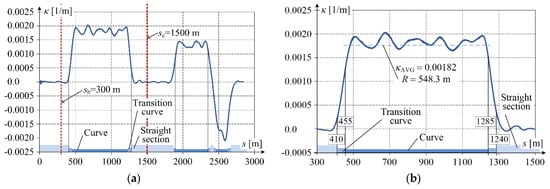
Figure 12.
Track curvature determined from PL-2000 coordinates: (a) for the entire examined railway line section—selected details for the example section from sb = 300 m to se = 1500 m are shown in figure b; (b) expanded fragment of a circular arc with transition curves, against data from the documentation on transition points between straight sections and transition curves, i.e., 410, 455, 1240, and 1285 m, and arc with radius R = 550 m.
As mentioned above, the variability analysis of the numerically determined curvature as a function of the examined track section length may be used for identifying straight sections, arcs, and transition curves. The curvature of the straight section equals zero, while for the arc it is constant and related to its radius. The curvature of the transition curve changes depending on its type. Fluctuations of curvature values make the unambiguous interpretation more complicated. A technique that is frequently used in this case is the linear section approximation making use of the least squares method with thresholding [34,35]. It should be stressed that the linear waveform of curvature along the transition curve corresponds only to the curve having the form of a clothoid. The results of identification completed using the least squares method for the numerically determined curvature shown in Figure 12a are given in Table 1.

Table 1.
Results of railway line section geometry identification.
Along with extending the measuring capabilities to situations when the GNSS signal quality is lost, the application of the INS unit in the measuring system provides an opportunity for using the lateral inclination angle signal in algorithms identifying the track geometry. The results of the railway line section geometry identification based on the lateral inclination angle αt carried out in the same way as for the curvature (Figure 10a), are given in Table 1. For comparison, the railway line curvature taken from the design documentation is also included.
The presented analysis has demonstrated that the numerically calculated curvature can be effectively used for determining the radii of circular arcs. Change in the measured lateral inclination angles which results from the presence of cants used on horizontal arcs of the railway line (cant transitions along transition curves and constant cant values on circular arcs) does not require advanced algorithms to calculate derivatives. However, the applicability of the lateral angle variability analysis for identifying railway track geometry elements in the horizontal plane is limited by the possible presence of arcs for which the cant was either not designed or not constructed or both. For this reason, an effective approach can be the integration of the curvature variability analysis with the lateral angle variability analysis, which will combine the advantages of these two approaches.
Comparing the results in Table 1 reveals some divergences, especially in the lengths of the identified sections. For a relatively short straight section between the transition curves linking two reverse circular arcs no. 2 and 3, the lateral angle variability analysis gives better results, compared to the documentation as a reference. The observed discrepancies result in part from the imperfection of the applied identification method and uncertainty of measurement, and in part from possible, relatively large differences between the real track and its documentation. The measurement uncertainty was determined by comparing the results of a mobile GNSS measurement with static measurements carried out according to standard geodetic methods [40]. It is advisable to continue the research of methods used for track geometry identification in the horizontal plane via evaluating curvature variability along the track axis. With the use of optimization techniques, this method will enable a more precise approximation of the measured and analyzed railway track sections. The need for increased precision in determining railway track geometry results directly from high requirements concerning railway lines against other transport routes [33,34].
6. Conclusions
Mobile measurements performed to determine the railway track axis using the GNSS technique are a useful tool for determining and estimating the geometry of the railway track during its operation. It is advisable to use GNSS receivers with 20 Hz frequency in combination with final data post-processing. The use of two receivers provides an opportunity for additionally determining the base vector, which facilitates the estimation of the obtained results’ quality.
The performed multiple measurements have demonstrated high accuracy of the obtained results, which shows their potential for determining the shape and position of the railway track axis with high precision, especially when introducing corrections for the lateral and longitudinal inclination of the track and platform motion on it.
The reconstruction of the railway line geometry, including its segmentation into straight sections and arcs, can be obtained using the Whittaker and Savitzky–Golay filtering algorithms. The application of the IMU/INS unit for extremely precise angle measurements enables the introduction of corrections to the coordinates recorded by the receivers (Figure 3) and supports identifying track geometry elements.
Currently, works are in progress by the authors to develop an algorithm for data fusion of the calculated curvature with the lateral inclination angle and direction angle of the track recorded by the INS system on the Y, X plane of the PL-2000 coordinate system. The developed algorithm, which will automatically reconstruct track geometry from mobile GNSS/INS measurements, is intended to support design processes and track maintenance performed by the railway infrastructure manager.
Author Contributions
Conceptualization: A.W., W.K., K.K. and S.J.; methodology: S.J. and K.K.; software: S.J.; validation: S.J. and J.S.; formal analysis: S.J. and K.K.; investigation: A.W., W.K., K.K., S.J., P.C., J.S. (Jacek Skibicki), S.G., J.S. (Jacek Szmaglinski), M.M, R.L., L.L. and A.S.; resources: A.W., W.K. and K.K.; data curation: S.J., K.K.; writing—original draft preparation: S.J. and K.K.; writing—review and editing: S.J. and K.K.; visualization: K.K.; supervision: W.K., J.S. (Jacek Szmaglinski) and A.W. All authors have read and agreed to the published version of the manuscript.
Funding
The research project entitled “Developing an innovative method to determine the precise rail vehicle trajectory” is co-financed by the European Fund for Regional Development within the framework of the Operational Programme Smart Growth 2014–2020 (POIR.04.01.01-00-0017/17-00) and by PKP Polskie Linie Kolejowe S.A. It is carried out within the framework of a joint undertaking entitled “BRIK—Research and Development in Railway Infrastructure”. The BRIK support program is jointly operated by the National Centre for Research and Development and PKP Polskie Linie Kolejowe S.A. Project acronym: InnoSatTrack.
Conflicts of Interest
The authors declare no conflict of interest.
References
- Tzanakakis, K. The Railway Track and Its Long Term Behaviour a Handbook for a Railway Track of High Quality; Springer: Berlin/Heidelberg, Germany, 2015. [Google Scholar]
- Escalona, J.L.; Urda, P.; Muñoz, S. A Track Geometry Measuring System Based on Multibody Kinematics, Inertial Sensors and Computer Vision. Sensors 2021, 21, 683. [Google Scholar] [CrossRef] [PubMed]
- Gao, Y.; Qian, S.; Li, Z.; Wang, P.; Wang, F.; He, Q. Digital Twin and Its Application in Transportation Infrastructure. In Proceedings of the 2021 IEEE 1st International Conference on Digital Twins and Parallel Intelligence (DTPI), Beijing, China, 15 July–15 August 2021; IEEE: Beijing, China, 2021; pp. 298–301. [Google Scholar] [CrossRef]
- Kostrzewski, M.; Melnik, R. Condition Monitoring of Rail Transport Systems: A Bibliometric Performance Analysis and Systematic Literature Review. Sensors 2021, 21, 4710. [Google Scholar] [CrossRef] [PubMed]
- Minea, M.; Dumitrescu, C.M.; Dima, M. Robotic Railway Multi-Sensing and Profiling Unit Based on Artificial Intelligence and Data Fusion. Sensors 2021, 21, 6876. [Google Scholar] [CrossRef] [PubMed]
- Otegui, J.; Bahillo, A.; Lopetegi, I.; Diez, L.E. Evaluation of Experimental GNSS and 10-DOF MEMS IMU Measurements for Train Positioning. IEEE Trans. Instrum. Meas. 2019, 68, 269–279. [Google Scholar] [CrossRef]
- Chiou, S.-B.; Yen, J.-Y. Precise Railway Alignment Measurements of the Horizontal Circular Curves and the Vertical Parabolic Curves Using the Chord Method. Proc. Inst. Mech. Eng. Part F J. Rail Rapid Transit 2019, 233, 537–549. [Google Scholar] [CrossRef]
- Kampczyk, A. Magnetic-Measuring Square in the Measurement of the Circular Curve of Rail Transport Tracks. Sensors 2020, 20, 560. [Google Scholar] [CrossRef]
- Jiang, Q.; Wu, W.; Jiang, M.; Li, Y. A New Filtering and Smoothing Algorithm for Railway Track Surveying Based on Landmark and IMU/Odometer. Sensors 2017, 17, 1438. [Google Scholar] [CrossRef]
- Li, R.; Bai, Z.; Chen, B.; Xin, H.; Cheng, Y.; Li, Q.; Wu, F. High-Speed Railway Track Integrated Inspecting by GNSS-INS Multisensor. In Proceedings of the 2020 IEEE/ION Position, Location and Navigation Symposium (PLANS), Portland, OR, USA, 20–23 April 2020; IEEE: Portland, OR, USA, 2020; pp. 798–809. [Google Scholar] [CrossRef]
- Naganuma, Y.; Yada, T.; Uematsu, T. Development of an Inertial Track Geometry Measuring Trolley and Utilization of Its Highprecision Data. Int. J. Transp. Dev. Integr. 2019, 3, 271–285. [Google Scholar] [CrossRef]
- Sánchez, A.; Bravo, J.L.; González, A. Estimating the Accuracy of Track-Surveying Trolley Measurements for Railway Maintenance Planning. J. Surv. Eng. 2017, 143, 05016008. [Google Scholar] [CrossRef]
- Zhang, Q.; Chen, Q.; Niu, X.; Shi, C. Requirement Assessment of the Relative Spatial Accuracy of a Motion-Constrained GNSS/INS in Shortwave Track Irregularity Measurement. Sensors 2019, 19, 5296. [Google Scholar] [CrossRef]
- Chen, Q.; Niu, X.; Zuo, L.; Zhang, T.; Xiao, F.; Liu, Y.; Liu, J. A Railway Track Geometry Measuring Trolley System Based on Aided INS. Sensors 2018, 18, 538. [Google Scholar] [CrossRef] [PubMed]
- Shankar, S.; Roth, M.; Schubert, L.A.; Verstegen, J.A. Automatic Mapping of Center Line of Railway Tracks Using Global Navigation Satellite System, Inertial Measurement Unit and Laser Scanner. Remote Sens. 2020, 12, 411. [Google Scholar] [CrossRef]
- Zhang, X.; Cui, X.; Huang, B. The Design and Implementation of an Inertial GNSS Odometer Integrated Navigation System Based on a Federated Kalman Filter for High-Speed Railway Track Inspection. Appl. Sci. 2021, 11, 5244. [Google Scholar] [CrossRef]
- Zhou, Y.; Chen, Q.; Niu, X. Kinematic Measurement of the Railway Track Centerline Position by GNSS/INS/Odometer Integration. IEEE Access 2019, 7, 157241–157253. [Google Scholar] [CrossRef]
- Chang, L.; Sakpal, N.P.; Elberink, S.O.; Wang, H. Railway Infrastructure Classification and Instability Identification Using Sentinel-1 SAR and Laser Scanning Data. Sensors 2020, 20, 7108. [Google Scholar] [CrossRef]
- Wang, Y.; Wang, L.; Hu, Y.H.; Qiu, J. RailNet: A Segmentation Network for Railroad Detection. IEEE Access 2019, 7, 143772–143779. [Google Scholar] [CrossRef]
- Weston, P.; Roberts, C.; Yeo, G.; Stewart, E. Perspectives on Railway Track Geometry Condition Monitoring from In-Service Railway Vehicles. Veh. Syst. Dyn. 2015, 53, 1063–1091. [Google Scholar] [CrossRef]
- Ai, C.; Tsai, Y. Automatic Horizontal Curve Identification and Measurement Method Using GPS Data. J. Transp. Eng. 2015, 141, 04014078. [Google Scholar] [CrossRef]
- Wilk, A.; Koc, W.; Specht, C.; Skibicki, J.; Judek, S.; Karwowski, K.; Chrostowski, P.; Szmagliński, J.; Dąbrowski, P.; Czaplewski, K.; et al. Innovative Mobile Method to Determine Railway Track Axis Position in Global Coordinate System Using Position Measurements Performed with GNSS and Fixed Base of the Measuring Vehicle. Measurement 2021, 175, 109016. [Google Scholar] [CrossRef]
- Wilk, A.; Specht, C.; Karwowski, K.; Koc, W.; Skibicki, J.; Czaplewski, K.; Chrostowski, P.; Dąbrowski, P.; Grulkowski, S.; Judek, S.; et al. Correction of Determined Coordinates of Railway Tracks in Mobile Satellite Measurements. Diagnostyka 2020, 21, 77–85. [Google Scholar] [CrossRef]
- Wilk, A.; Koc, W.; Specht, C.; Judek, S.; Karwowski, K.; Chrostowski, P.; Czaplewski, K.; Dabrowski, P.S.; Grulkowski, S.; Licow, R.; et al. Digital Filtering of Railway Track Coordinates in Mobile Multi–Receiver GNSS Measurements. Sensors 2020, 20, 5018. [Google Scholar] [CrossRef]
- Aceituno, J.F.; Chamorro, R.; Muñoz, S.; Escalona, J.L. An Alternative Procedure to Measure Railroad Track Irregularities. Application to a Scaled Track. Measurement 2019, 137, 417–427. [Google Scholar] [CrossRef]
- Khosravi, M.; Soleimanmeigouni, I.; Ahmadi, A.; Nissen, A. Reducing the Positional Errors of Railway Track Geometry Measurements Using Alignment Methods: A Comparative Case Study. Measurement 2021, 178, 109383. [Google Scholar] [CrossRef]
- Taheri Andani, M.; Peterson, A.; Munoz, J.; Ahmadian, M. Railway Track Irregularity and Curvature Estimation Using Doppler LIDAR Fiber Optics. Proc. Inst. Mech. Eng. Part F J. Rail Rapid Transit 2018, 232, 63–72. [Google Scholar] [CrossRef]
- Zhu, F.; Zhou, W.; Zhang, Y.; Duan, R.; Lv, X.; Zhang, X. Attitude Variometric Approach Using DGNSS/INS Integration to Detect Deformation in Railway Track Irregularity Measuring. J. Geod. 2019, 93, 1571–1587. [Google Scholar] [CrossRef]
- Eilers, P.H.C. A Perfect Smoother. Anal. Chem. 2003, 75, 3631–3636. [Google Scholar] [CrossRef]
- Roy, I.G. An Optimal Savitzky–Golay Derivative Filter with Geophysical Applications: An Example of Self-potential Data. Geophys. Prospect. 2020, 68, 1041–1056. [Google Scholar] [CrossRef]
- Elberink, S.; Khoshelham, K. Automatic Extraction of Railroad Centerlines from Mobile Laser Scanning Data. Remote Sens. 2015, 7, 5565–5583. [Google Scholar] [CrossRef]
- Li, W.; Pu, H.; Schonfeld, P.; Song, Z.; Zhang, H.; Wang, L.; Wang, J.; Peng, X.; Peng, L. A Method for Automatically Recreating the Horizontal Alignment Geometry of Existing Railways: Recreating the Horizontal Alignment of Existing Railways. Comput.-Aided Civ. Infrastruct. Eng. 2019, 34, 71–94. [Google Scholar] [CrossRef]
- Luo, W.; Li, L. Automatic Geometry Measurement for Curved Ramps Using Inertial Measurement Unit and 3D LiDAR System. Autom. Constr. 2018, 94, 214–232. [Google Scholar] [CrossRef]
- AL-Qadri, M.; Cheng, J.; Zhang, Y. Semi-Automatic Extraction of Geometric Elements of Curved Ramps from Google Earth Images. Sustainability 2022, 14, 1001. [Google Scholar] [CrossRef]
- Easa, S.M.; Wang, F. Fitting Composite Horizontal Curves Using the Total Least-Squares Method. Surv. Rev. 2011, 43, 67–79. [Google Scholar] [CrossRef]
- Koc, W.; Wilk, A.; Specht, C.; Karwowski, K.; Skibicki, J.; Czaplewski, K.; Judek, S.; Chrostowski, P.; Szmagliński, J.; Dąbrowski, P.; et al. Determining horizontal curvature of railway track axis in mobile satellite measurements. Bull. Pol. Acad. Sci. Tech. Sci. 2021, 69, 1–10. [Google Scholar] [CrossRef]
- Lamas, D.; Soilán, M.; Grandío, J.; Riveiro, B. Automatic Point Cloud Semantic Segmentation of Complex Railway Environments. Remote Sens. 2021, 13, 2332. [Google Scholar] [CrossRef]
- Pu, H.; Zhao, L.; Li, W.; Zhang, J.; Zhang, Z.; Liang, J.; Song, T. A Global Iterations Method for Recreating Railway Vertical Alignment Considering Multiple Constraints. IEEE Access 2019, 7, 121199–121211. [Google Scholar] [CrossRef]
- Soilán, M.; Nóvoa, A.; Sánchez-Rodríguez, A.; Justo, A.; Riveiro, B. Fully Automated Methodology for the Delineation of Railway Lanes and the Generation of IFC Alignment Models Using 3D Point Cloud Data. Autom. Constr. 2021, 126, 103684. [Google Scholar] [CrossRef]
- Szmagliński, J.; Wilk, A.; Koc, W.; Karwowski, K.; Chrostowski, P.; Skibicki, J.; Grulkowski, S.; Judek, S.; Licow, R.; Makowska-Jarosik, K.; et al. Verification of Satellite Railway Track Position Measurements Making Use of Standard Coordinate Determination Techniques. Remote Sens. 2022, 14, 1855. [Google Scholar] [CrossRef]


Publisher’s Note: MDPI stays neutral with regard to jurisdictional claims in published maps and institutional affiliations. |
© 2022 by the authors. Licensee MDPI, Basel, Switzerland. This article is an open access article distributed under the terms and conditions of the Creative Commons Attribution (CC BY) license (https://creativecommons.org/licenses/by/4.0/).