Fusing Hyperspectral and Multispectral Images via Low-Rank Hankel Tensor Representation

Abstract

Hyperspectral images (HSIs) have high spectral resolution and low spatial resolution. HSI super-resolution (SR) can enhance the spatial information of the scene. Current SR methods have generally focused on the direct utilization of image structure priors, which are often modeled in global or local lower-order image space. The spatial and spectral hidden priors, which are accessible from higher-order space, cannot be taken advantage of when using these methods. To solve this problem, we propose a higher-order Hankel space-based hyperspectral image-multispectral image (HSI-MSI) fusion method in this paper. In this method, the higher-order tensor represented in the Hankel space increases the HSI data redundancy, and the hidden relationships are revealed by the nonconvex penalized Kronecker-basis-representation-based tensor sparsity measure (KBR). Weighted 3D total variation (W3DTV) is further applied to maintain the local smoothness in the image structure, and an efficient algorithm is derived under the alternating direction method of multipliers (ADMM) framework. Extensive experiments on three commonly used public HSI datasets validate the superiority of the proposed method compared with current state-of-the-art SR approaches in image detail reconstruction and spectral information restoration.

1. Introduction

The hyperspectral (HS) remote sensing technique, which emerged in the 1980s, is a comprehensive scientific technique combining information processing, computer technology and other technologies. Hyperspectral images (HSIs) consist of dozens to hundreds of spectral bands in the same area of the Earth’s surface. HSIs have the characteristics of high dimensionality, high redundant band information and high spectral resolution. Compared to traditional remote sensing techniques, hyperspectral remote sensing techniques can be used to qualitatively and quantitatively detect substances with ultrastrong spectral information. The advantage of HSIs lies in their high spectral resolution. In HSIs, many bands are required to increase the physical size of the photoreceptor, spatial resolution is sacrificed as a result. However, high spatial resolution images are required in many applications of HS remote sensing, such as marine research [1,2], food detection [3], military [4] and other fields [5,6,7,8,9]. Therefore, research on super-resolution (SR) reconstruction technology for HSIs has important scientific significance and engineering application value.

Recent studies of HSI SR can be divided into four types: Bayesian framework [10,11,12,13], matrix factorization [14,15,16,17], tensor factorization [18,19,20,21], and deep learning [22,23,24].

The Bayesian framework is a common method that is used to establish the posterior distribution of high spatial resolution hyperspectral image (HR-HSI) based on prior information and observational models. In [10], a multi-sparse Bayesian learning method was proposed based on the sparsity prior and the temporal correlation between successive frames. Wei et al. [11] adopted a Bayesian model based on sparse coding and dictionary learning to solve the fusion problem. The maximum a posterior (MAP) estimator, which uses a coregistered HSI from an auxiliary sensor, was introduced in [12]. In [13], a Bayesian sparse representation and spectral decomposition fusion method was adopted to improve image resolution. Bayesian-based methods are very sensitive to the independence of input data, which limits the practical application of the Bayesian framework.

Matrix factorization-based methods usually decompose HSI into two matrix forms to represent the spectral dictionary and low retention numbers. These two matrices are estimated by observing HS-multispectral (HS-MS) pairs. In [14], a spectral matrix decomposition and dictionary learning method was proposed to train spectral dictionaries of high spatial-spectral information by low spatial resolution HSI (LR-HSI) and HR multispectral image (HR-MSI) matrices. In [15], a spatial-spectral sparse representation method was adopted by using spectral decomposition priors, sparse priors and nonlocal self-similarity. In [16], a non-negative structure sparse representation (NSSR) method based on the sparsity of HR-HSI was proposed for the joint estimation of the HS dictionary and sparse code. In [17], based on sparse representation and local spatial low-rank, a method was proposed to solve HSI SR by estimating spectral dictionary and regression coefficients. Hyperspectral data are three-dimensional images, which have one more dimension of spectral information than ordinary two-dimensional images. Matrix-based methods destroy the data structure.

As multidimensional arrays, tensors provide a natural expression of HSI data. Tensor representation has been widely applied to high-dimensional data denoising [25,26,27,28], completion [29,30,31] and SR [18,19,20,21] in the past few years. A coupled non-negative tensor decomposition (NTD) method was introduced in [18] to extend the non-negative matrix decomposition to a tensor. In this method, Tucker decomposition of LR-HSI and HR-MSI is performed under NTD constraints. A joint tensor decomposition (JTF)-based method for solving HR-HSI was proposed by Ren et al. [19]. These methods are designed by treating the HSI data as a 3rd-order tensor and assuming that the tensor is of sufficiently global low-rank. Nonlocal self-similarity is an important feature of images. It depicts the repeated appearance of the nonlocal regional structure of the image, effectively retains the edge information of the image, and has certain advantages in image restoration. Dian et al. [20] adopted a fusion method based on low tensor train rank (LTTR) decomposition. This method was applied to HR-HSI through the nonlocal similarity learned from HR-MSI, and multiple group 4D similarity cubes were formed. The SR problem was efficiently solved using LTTR priors for the 4D cubes. In [21], a fusion method based on nonlocal Tucker decomposition, which uses the nonlocal similarity of HS data, was proposed. The clustering blocks obtained by nonlocal self-similarity are very dependent on the accuracy of block matching. The nonlocal clustering space does not improve the data redundancy, which makes it difficult to effectively explore the low-rank characteristics contained in the data.

With its superior effect in detection, recognition, classification and other tasks [32,33,34,35,36,37,38,39], deep learning has been gradually applied to deal with low-level vision tasks in recent years [22,23,24]. Bing et al. [22] proposed an improved generative adversarial network (GAN) to improve the squeeze and excitation (SE) block. By increasing the weight value of important features and reducing the weight value of weak features, the SE block is included in the simplified enhanced deep residual networks for the single image SR (SISR) model to recover HSIs. To improve the computing speed of deep learning networks, Kim et al. [23] designed an SISR network, which improves the fire modules based on Squeeze-Net, and asymmetrically arranges the fire modules. The number of network parameters is effectively reduced. In [24], a video SR network based on learning temporal dynamics was introduced. In this network, filters with different temporal scales are used to fully exploit the temporal relationship of continuous LR frames, and a spatial alignment network is employed to reduce motion complexity. The performance of deep learning networks is closely determined by the size of the training data. However, the size of the acquired HSI data is limited by the physical size of the photosensor, and there are only dozens to hundreds of spectral bands, which is not sufficient for training.

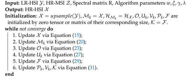
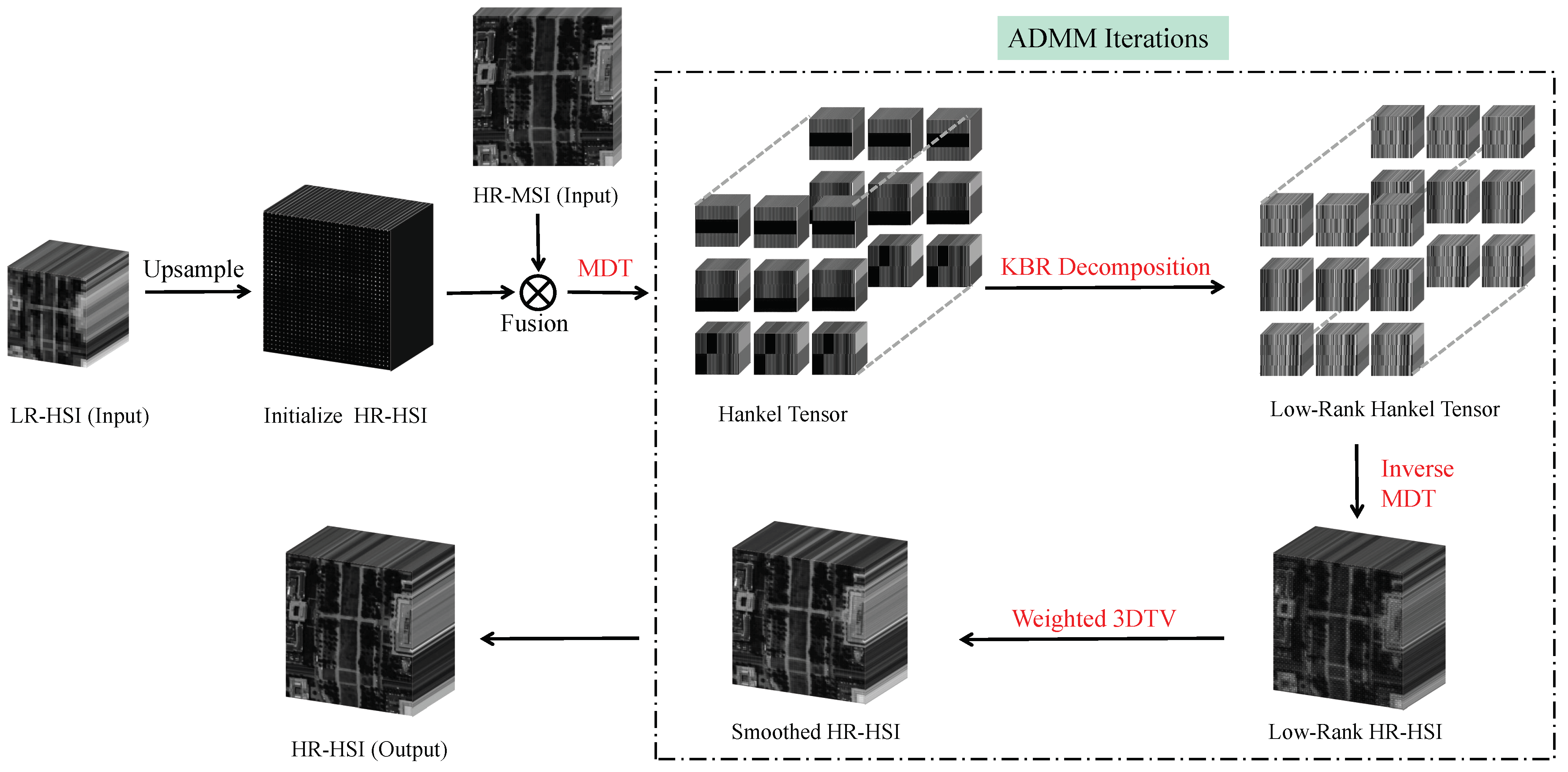
Considering the limitation of HSI data and to better maintain the data structure, we adopt a tensor-based method. To improve data redundancy and fully explore the low-rank characteristics of data, we propose using HSIs in the Hankel space to carry out high-order low-rank tensor SR (HTSR). The Hankel space is an embedded space obtained by employing delay-embedding transform in a multi-way manner for tensors, which consists of duplicated high-order tensors with low-rankness. Different from traditional high-order tensor decomposition, we use a folded-concave penalized Kronecker-basis-representation-based tensor sparsity measure (KBR) tensor decomposition [40] to reasonably and effectively represent the low-rank properties of high-order tensor in the Hankel space. From the spatial-spectral domain of HS data, there are local smoothing characteristics between adjacent pixels. We adopt W3DTV to constrain the spatial-spectral local continuity of HSIs. To further improve the effect of HSI SR recovery, HSI-MSI fusion is used in our method. Unlike HSIs, multispectral images (MSIs) contain 3–20 discontinuous bands with a higher signal-to-noise ratio (SNR) and spatial resolution. HR-MSI-assisted enhancement can compensate for the lack of LR-HSI, so the fusion method can more accurately reconstruct HR-HSI.

The contributions are highlighted as follows:

• To exploit the low-rank information hidden in HSI data, we propose modeling the SR problem in the Hankel space. Compared with the global and nonlocal image spaces, the effectiveness of the designed Hankel space SR has been demonstrated.
• A folded-concave penalized KBR tensor decomposition is proposed to describe the low-rank characteristics in the spatial–spectral domain of the high-order tensor in the Hankel space.
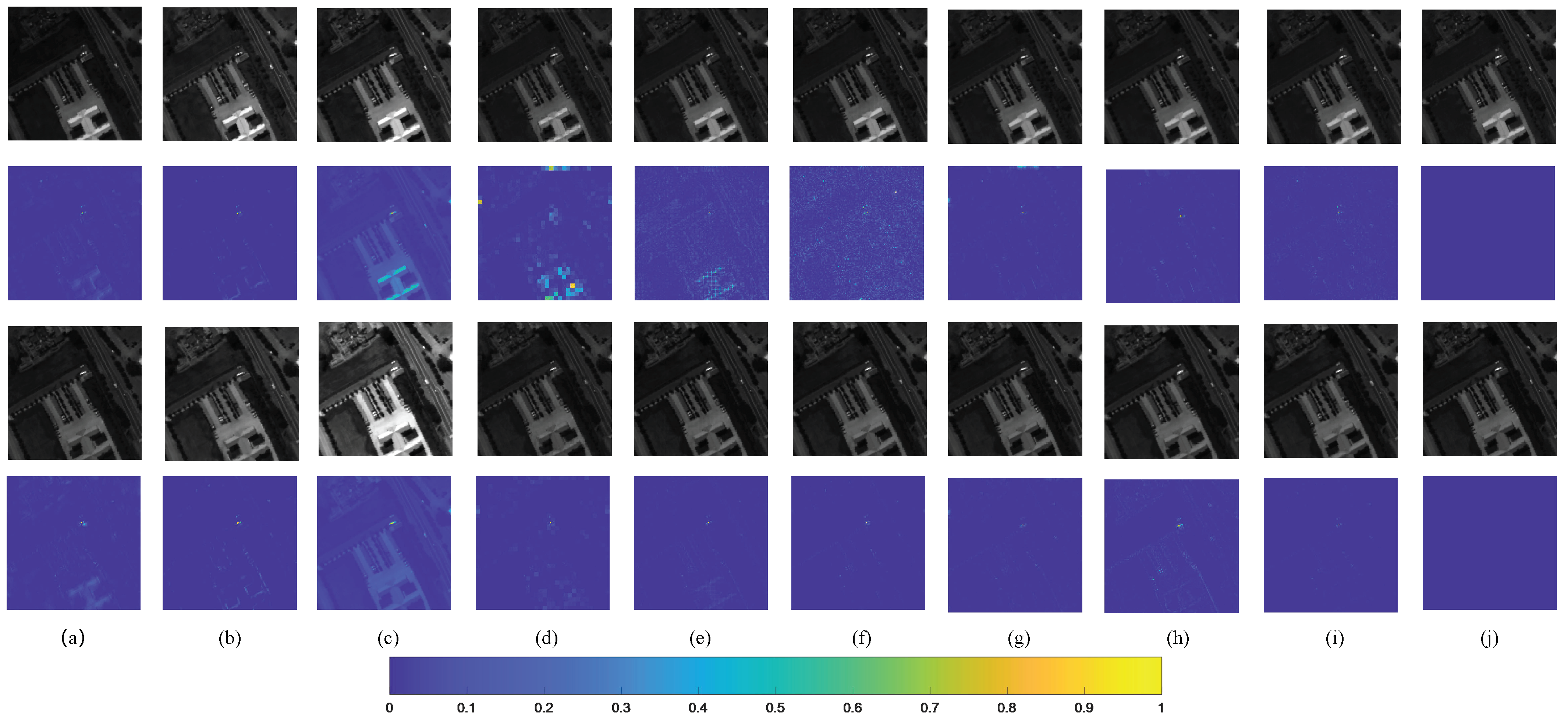
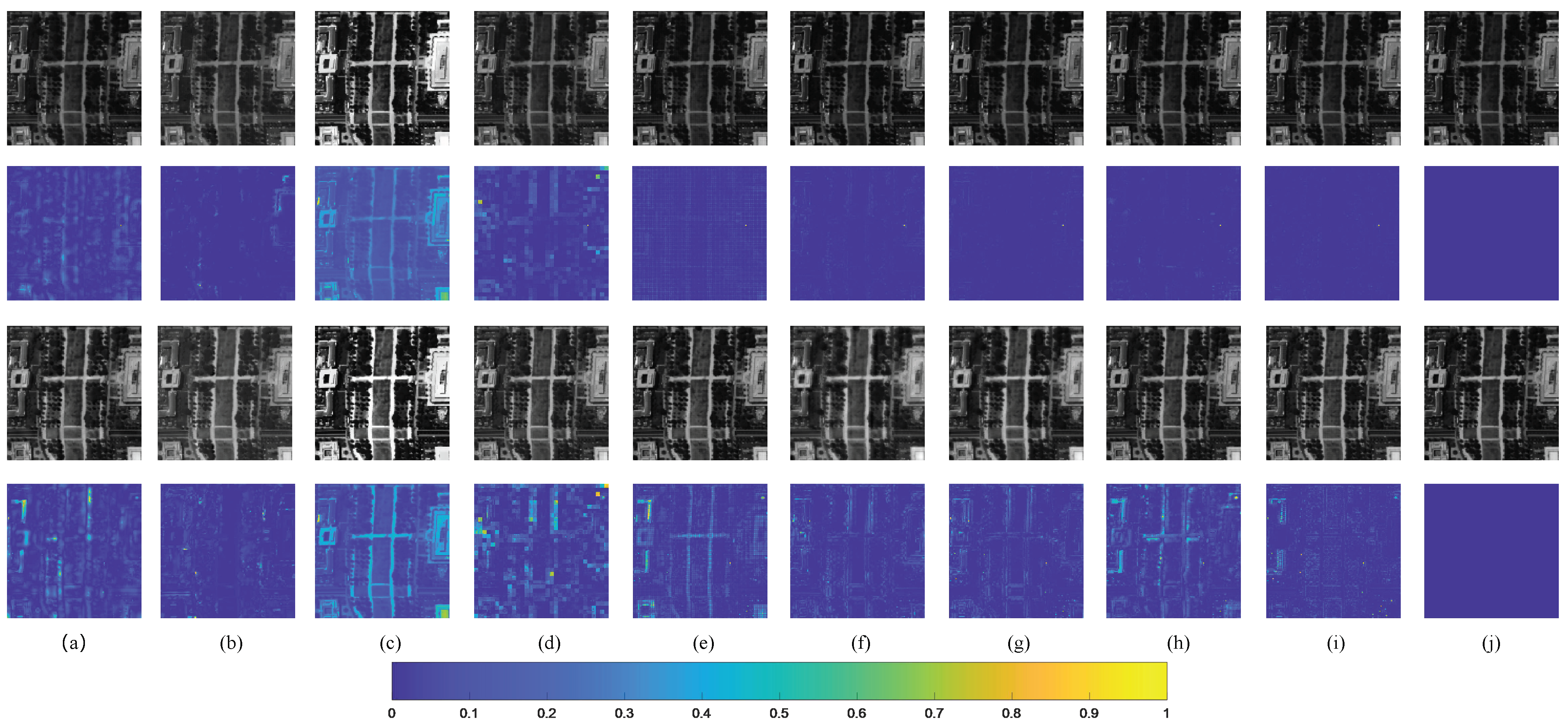
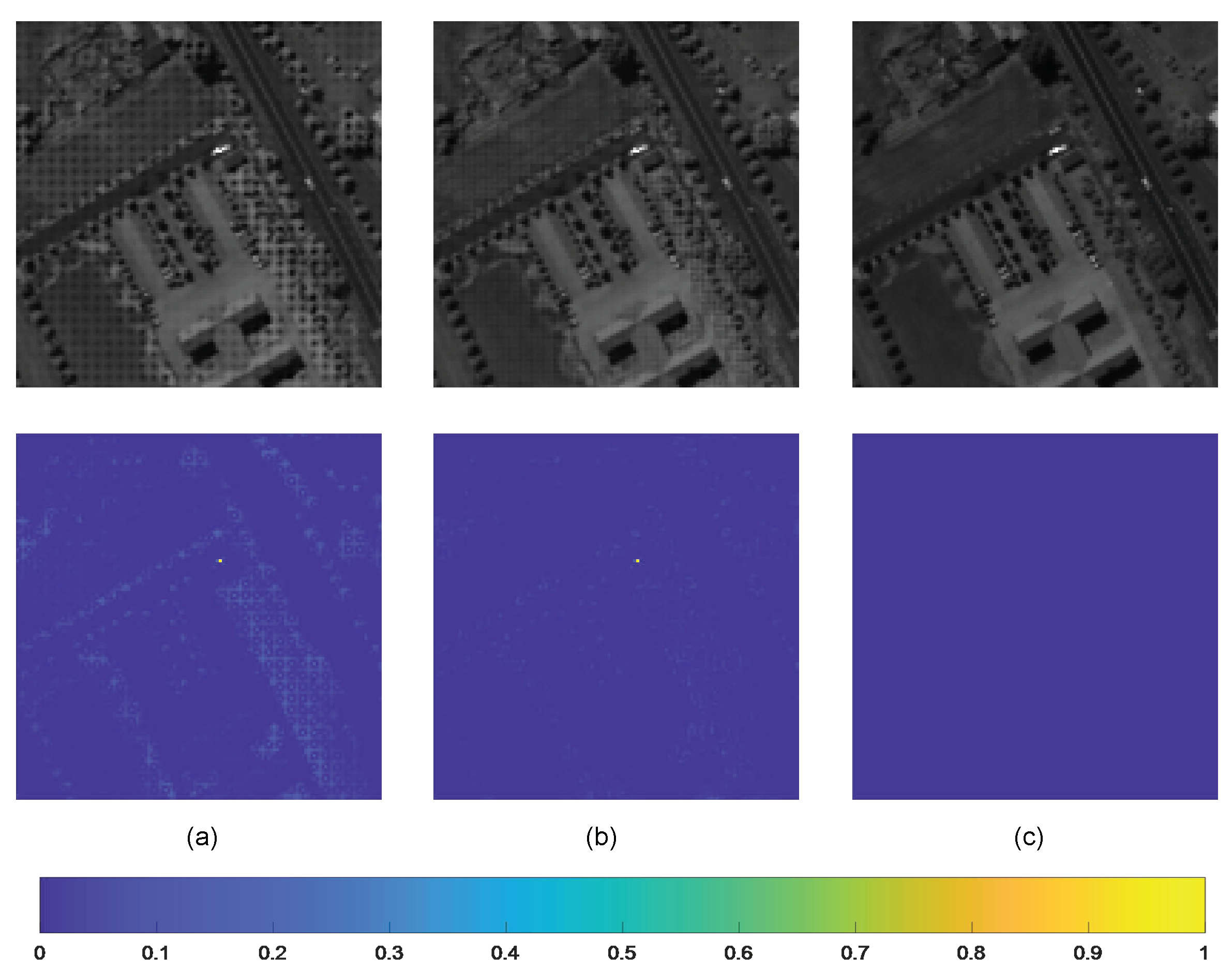
• Extensive experiments demonstrate that our HTSR method can obtain a relatively great performance compared with the current state-of-the-art methods.

The rest of this paper is organized as follows. In Section 2, we introduce the tensor preparatory knowledge. In Section 3, we present the proposed HTSR fusion method. In Section 4, we introduce the optimization problem of the solution algorithm of the HTSR method in detail. The experimental results on three commonly used hyperspectral datasets are described in Section 5. Finally, conclusions are presented in Section 6.

2. Notions and Preliminaries on Tensors

A tensor is a multidimensional array, and a given tensor of order N is denoted as $\mathcal{X}\in {\mathbb{R}}^{I_1\times I_2\times \cdots \times I_N}$. The related operations of the tensor are introduced in

Table 1. Tensor notations and operations.

Notation	Definition
$x,\mathbf{x},X,\mathcal{X}$	scalar, vector, matrix, tensor
$x_{i_1,i_2,\dots ,i_N}$	tensor element
${\mathcal{X}}_{:,i_2,i_3,\dots ,i_N}$	tensor fiber
${\mathcal{X}}_{:,:,i_3,\dots ,i_N}$	tensor slice
$\mathcal{Y}=\mathcal{X}{\times }_{n}U$	tensor mode$-n$ product
${\mathcal{X}}_{\left(n\right)}$ or $unfol{d}_n\left(\mathcal{X}\right)$	tensor mode$-n$ matrix
$fol{d}_n\left({\mathcal{X}}_{\left(n\right)}\right)$	the inverse operation of $unfol{d}_n\left(\mathcal{X}\right)$
$r_n=rank\left({\mathcal{X}}_{\left(n\right)}\right)$	multilinear rank
$\mathcal{X}=\mathcal{G}{\times }_1{U}^1{\times }_2{U}^2···{\times }_N{U}^N$	Tucker decomposition
$\mathcal{X}={\sum }_r^R{\mathbf{x}}_r^{\left(1\right)}\circ {\mathbf{x}}_r^{\left(2\right)}\circ \cdots \circ {\mathbf{x}}_r^{\left(N\right)}$	CP decomposition
$\langle \mathcal{X},\mathcal{Y}\rangle$	inner product
${\parallel \mathcal{X}\parallel }_0$	${\ell }_0$ norm
${\parallel \mathcal{X}\parallel }_1$	${\ell }_1$ norm
${\parallel \mathcal{X}\parallel }_F$	${\ell }_F$ norm

.

3. HSI-MSI Fusion Problem Formulation

In this section, the HTSR method for HR-HSI SR is presented. The main framework of HTSR is shown in Figure 1.

3.1. Observation Model

In this paper, all HR-HSI, HR-MSI, and LR-HSI are denoted as 3D tensors. The target HR-HSI is denoted as $\mathcal{X}\in {\mathbb{R}}^{W\times H\times B}$, where W and H represent the spatial size of the spatial mode and B represents the band size of the spectral mode. LR-HSI is denoted as $\mathcal{Y}\in {\mathbb{R}}^{w\times h\times B}$. Through spatial blurring and downsampling from $\mathcal{X}$, $\mathcal{Y}$ can be obtained as follows:

$$\mathcal{Y}=DS\mathcal{X}$$

(1)

where S is the blurring operator and D is the downsampling operator.

$\mathcal{Z}\in {\mathbb{R}}^{W\times H\times b}$ denotes the acquired HR-MSI of the same scene, where b represents the spectral bands. Through downsampling from $\mathcal{X}$ along the spectral mode, $\mathcal{Z}$ can be modeled as

$$\mathcal{Z}=\mathcal{X}{\times }_{3}R$$

(2)

where $R\in {\mathbb{R}}^{b\times B}$ represents the spectral response matrix.

3.2. Multi-Way Delay-Embedding Transform on HR-HSI

Traditionally, global or nonlocal low-rank techniques are used to model direct correlations in data. These techniques are insufficient for exploiting indirect correlations hidden in data. To better employ the low-rank correlations hidden in $\mathcal{X}$, we map it to the Hankel space. We perform Hankel processing on all modes of $\mathcal{X}$ to acquire Hankel tensor ${\mathcal{H}}_{\mathcal{X}}$ via multi-way delay-embedding transform (MDT) [41]. The Hankel tensor ${\mathcal{H}}_{\mathcal{X}}$ can be obtained via MDT with an N-th order tensor $\mathcal{X}$ and $\xi \in {\mathbb{R}}^N$ as follows:

$${\mathcal{H}}_{\xi }\left(\mathcal{X}\right)=fold{}_{(I,\xi )}(\mathcal{X}{\times }_1{J}_1\cdots {\times }_N{J}_N)$$

(3)

where a 2N-th order tensor from the input N-th order tensor is constructed by $fold{}_{(I,\xi )}:{\mathbb{R}}^{{\xi }_1(I_1-{\xi }_1+1)\times \cdots \times {\xi }_N(I_N-{\xi }_N+1)}\to {\mathbb{R}}^{{\xi }_1\times (I_1-{\xi }_1+1)\times \cdots \times {\xi }_N\times (I_N-{\xi }_N+1)}$, $J_n\in {\left\{0,1\right\}}^{{\xi }_n(I_n-{\xi }_n+1)\times I_n}$ ($n\in [1,N]$) is a duplication matrix. The inverse MDT for Hankel tensor ${\mathcal{H}}_{\mathcal{X}}$ is defined by

$${\mathcal{H}}_{\xi }^{-1}\left({\mathcal{H}}_{\mathcal{X}}\right)=unfol{d}_{(I,\xi )}\left({\mathcal{H}}_{\mathcal{X}}\right){\times }_1{J}_1^{\perp }\cdots {\times }_N{J}_N^{\perp }$$

(4)

where $unfold{}_{(I,\xi )}=fol{d}_{(I,\xi )}^{-1}$, $J^{\perp }={\left(J^{T}J\right)}^{-1}{J}^T$.

The MDT is a combination of multi-way folding and multi-linear duplication operations. Thus, the Hankel tensor ${\mathcal{H}}_{\mathcal{X}}$ has the characteristic of high redundancy and is a high-order tensor. The KBR is more suitable for exploiting the low-rank information hidden in the high-order Hankel tensor. For a given N-dimensional tensor $\mathcal{X}\in {\mathbb{R}}^{I_1\times I_2\times \cdots \times I_N}$, its KBR decomposition can be represented as

$$S\left(\mathcal{X}\right)=t{∥\mathcal{O}∥}_0+(1-t){\displaystyle \prod _{j=1}^N}rank\left({\mathcal{X}}_{\left(j\right)}\right)$$

(5)

where $t\in [0,1]$ is used to balance the two terms in the equation and $\mathcal{O}\in {\mathbb{R}}^{r_1\times r_2\times \cdots \times r_N}$ is the core tensor of the Tucker decomposition of $\mathcal{X}$. The first term characterizes the number of non-zero elements in the nuclear tensor, and the second term characterizes the volume size of the non-zero square in the nuclear tensor.

Since the $l_0$ norm and the nuclear norm in Equation (5) are discrete measures, it is computationally difficult to directly model them, and it is necessary to reasonably relax them. Many studies have shown that it is easy to relax the $l_0$ norm and the nuclear norm [21,42,43] using the minimax concave plus (MCP) norm, which is very reasonable and can compensate for the biased estimates brought by $l_0$ norm modeling.

The MCP penalty is a typical folded-concave penalty as follows:

$${\psi }_{\lambda }\left(t\right)=\left\{\begin{array}{ll}\gamma {\lambda }^2/2,& if\left|t\right|\ge \gamma \lambda .\\ \lambda \left|t\right|-\frac{t^2}{2\gamma },& otherwise.\end{array}\right.$$

(6)

where $\gamma$ is a fixed constant.

To better approximate ${\mathcal{H}}_{\mathcal{X}}$, we adopt the MCP penalty as the sparsity constraint, and the above KBR sparse model is formulated as

$$S^{*}\left({\mathcal{H}}_{\mathcal{X}}\right)=M_{{\lambda }_1}\left(\mathcal{O}\right)+{\lambda }_3{\displaystyle \prod _{j=1}^N}{M}_{{\lambda }_2}^{*}\left({\mathcal{H}}_{{\mathcal{X}}_{\left(j\right)}}\right)$$

(7)

where $M_{{\lambda }_1}\left(\mathcal{O}\right)={\displaystyle \sum _{i,j,k}}{\psi }_{{\lambda }_1}\left({\mathcal{O}}_{i,j,k}\right)$, ${M^{*}}_{{\lambda }_2}\left({\mathcal{H}}_{{\mathcal{X}}_{\left(j\right)}}\right)={\displaystyle \sum _m}{\psi }_{{\lambda }_2}({\sigma }_m\left({\mathcal{H}}_{{\mathcal{X}}_{\left(j\right)}}\right))$, and ${\sigma }_m\left({\mathcal{H}}_{{\mathcal{X}}_{\left(j\right)}}\right)$ is the m-th singular value of ${\mathcal{H}}_{{\mathcal{X}}_{\left(j\right)}}$.

3.3. Weighted 3D Total Variation Regularization

Total variation (TV) regularization has been commonly applied to study the spatial piecewise smooth structure to address HSI restoration tasks [21,44,45]. Considering that HR-HSI is a 3D tensor and has a strong spatial-spectral continuity structure, we use a weighted 3DTV (W3DTV) term to explore the local smooth structure of $\mathcal{X}$ as follows:

$${∥\mathcal{X}∥}_{3DTV}=\sum _{a,b,c}{w}_1\left|x_{a,b,c}-x_{a,b,c-1}\right|+w_2\left|x_{a,b,c}-x_{a,b-1,c}\right|+w_3\left|x_{a,b,c}-x_{a-1,b,c}\right|$$

(8)

We obtain the following form:

$${∥\mathcal{X}∥}_{3DTV}={∥G_w\left(\mathcal{X}\right)∥}_1$$

(9)

where $G_w(·)=[w_1\times G_h(·);w_2\times G_v(·);w_3\times G_t(·)]$ is the weighted 3D difference operator. $G_h(·)$, $G_v(·)$ and $G_t(·)$ are the first-order difference operators along the three modes of the HSI cube.

3.4. HSI-MSI Fusion via HTSR

By integrating the regulation terms mentioned above (Equations (1), (2), (7) and (9)), we formulate the HSI-MSI fusion problem as

$$S^{*}\left({\mathcal{H}}_{\mathcal{X}}\right)+{\lambda }_4{∥\mathcal{Y}-DS\mathcal{X}∥}_F^2+{\lambda }_5{∥\mathcal{Z}-\mathcal{X}{\times }_{3}R∥}_F^2+{\lambda }_{TV}{∥\mathcal{X}∥}_{3DTV}$$

(10)

which is equal to

$$\begin{array}{l}{M}_{{\lambda }_1}\left(\mathcal{O}\right)+{\lambda }_3{\displaystyle \prod _{j=1}^N}{M}_{{\lambda }_2}^{*}\left({\mathcal{H}}_{{\mathcal{X}}_{\left(j\right)}}\right)+{\lambda }_4{∥\mathcal{Y}-DS\mathcal{X}∥}_F^2+{\lambda }_5{∥\mathcal{Z}-\mathcal{X}{\times }_{3}R∥}_F^2+{\lambda }_{TV}{∥G_w\left(\mathcal{X}\right)∥}_1\\ {\mathcal{H}}_{\mathcal{X}}=\mathcal{O}{\times }_1{U}_1\cdots {\times }_N{U}_N\end{array}$$

(11)

where ${\lambda }_1$, ${\lambda }_2$, ${\lambda }_3$, ${\lambda }_4$, ${\lambda }_5$ and ${\lambda }_{TV}$ are regularization parameters. This is a nonconvex optimization problem.

4. Optimization Procedure

4.1. Algorithm

Equation (11) is an unconstrained optimization problem. We propose an effective algorithm to solve it under the ADMM framework. By introducing two auxiliary variables $\mathcal{F}=G_w\left(\mathcal{X}\right)$ and $\mathcal{X}=\mathcal{M}$, we have

$$\begin{array}{c}\hfill M_{{\lambda }_1}\left(\mathcal{O}\right)+{\lambda }_3{\displaystyle \prod _{j=1}^N}{M}_{{\lambda }_2}^{*}\left({\mathcal{H}}_{{{\mathcal{M}}_j}_{\left(j\right)}}\right)+{\lambda }_4{∥\mathcal{Y}-DS\mathcal{X}∥}_F^2+{\lambda }_5{∥\mathcal{Z}-\mathcal{X}{\times }_{3}R∥}_F^2+{\lambda }_{TV}{∥\mathcal{F}∥}_1\hfill \\ \begin{array}{cc}s.t.& {\mathcal{H}}_{{\mathcal{M}}_j}=\mathcal{O}{\times }_1{U}_1\cdots {\times }_N{U}_N\end{array}\hfill \\ \begin{array}{cc}& \end{array}\mathcal{X}={\mathcal{M}}_j\hfill \\ \begin{array}{cc}& \end{array}\mathcal{F}=G_w\left(\mathcal{X}\right)\hfill \\ \begin{array}{cc}& \end{array}{U}_j^T{U}_j=I,j=1,\cdots ,N\hfill \end{array}$$

(12)

The corresponding augmented Lagrangian function is given as:

$$\begin{array}{l}L(\mathcal{X},\mathcal{M},\mathcal{O},U,\mathcal{F},\mathcal{K},\mathcal{P},\mathcal{V})\\ =M_{{\lambda }_1}\left(\mathcal{O}\right)+{\lambda }_3{\displaystyle \prod _{j=1}^N}{M}_{{\lambda }_2}^{*}\left({{\mathcal{H}}_{{\mathcal{M}}_j}}_{\left(j\right)}\right)+{\lambda }_{{}_4}{∥\mathcal{Y}-DS\mathcal{X}∥}_F^2+{\lambda }_5{∥\mathcal{Z}-\mathcal{X}{\times }_{3}R∥}_F^2\\ +{\lambda }_{TV}{∥\mathcal{F}∥}_1+〈\mathcal{F}-G_w\mathcal{X},\mathcal{K}〉+\frac{l}{2}{∥\mathcal{F}-G_w\mathcal{X}∥}_F^2+{\displaystyle \sum _{j=1}^N}〈\mathcal{X}-{\mathcal{M}}_j,{\mathcal{P}}_j〉\\ +{\displaystyle \sum _{j=1}^N}\frac{\mu }{2}{∥\mathcal{X}-{\mathcal{M}}_j∥}_F^2+{\displaystyle \sum _j^N}〈{\mathcal{H}}_{{\mathcal{M}}_j}-\mathcal{O}{\times }_1{U}_1\cdots {\times }_N{U}_N,{\mathcal{V}}_j〉\\ +{\displaystyle \sum _j^N}\frac{v}{2}{∥{\mathcal{H}}_{{\mathcal{M}}_j}-\mathcal{O}{\times }_1{U}_1\cdots {\times }_N{U}_N∥}_F^2\end{array}$$

(13)

where $\mathcal{K}$, ${\left\{\mathcal{P}\right\}}_{j=1}^N$ and ${\left\{\mathcal{V}\right\}}_{j=1}^N$ are the Lagrangian multipliers. $\mu$, v and l are the penalty parameters and $U_j^T{U}_j=I,\forall j=1,\cdots ,N$. Based on ADMM, we can minimize Equation (13) by solving the following subproblems:

Update $\mathcal{X}$. By fixing the other variables, Equation (13) leads to the following optimization problem:

$$\begin{array}{l}\begin{array}{cc}\mathcal{X}& =\end{array}\underset{\mathcal{X}}{argmin}\mathcal{L}(\mathcal{X},\mathcal{M},\mathcal{O},U,\mathcal{F},\mathcal{K},\mathcal{P},\mathcal{V})\\ \begin{array}{cc}& =\end{array}{\lambda }_{{}_4}{∥\mathcal{Y}-DS\mathcal{X}∥}_F^2+{\lambda }_5{∥\mathcal{Z}-\mathcal{X}{\times }_{3}R∥}_F^2+〈\mathcal{F}-G_w\mathcal{X},\mathcal{K}〉\\ \begin{array}{cc}& +\frac{l}{2}{∥\mathcal{F}-G_w\mathcal{X}∥}_F^2+{\displaystyle \sum _{j=1}^N}〈\mathcal{X}-{\mathcal{M}}_j,{\mathcal{P}}_j〉+{\displaystyle \sum _{j=1}^N}\frac{\mu }{2}{∥\mathcal{X}-{\mathcal{M}}_j∥}_F^2\end{array}\end{array}$$

(14)

which is equivalent to solving the following linear equation:

$$\begin{array}{l}2{\lambda }_4{\left(DS\right)}^{T}DS\mathcal{X}+\mu N\mathcal{X}+l{G}_w^{\prime }{G}_w\mathcal{X}+2{\lambda }_5\mathcal{X}\\ =2{\lambda }_4{\left(DS\right)}^T\mathcal{Y}+{\displaystyle \sum _{j=1}^N}(\mu {\mathcal{M}}_j-{\mathcal{P}}_j)+l{G}_w^{\prime }\mathcal{F}+G_w^{\prime }\mathcal{K}+2{\lambda }_5\left(\mathcal{Z}{\times }_3{R}^T\right)\end{array}$$

(15)

where ${\left(DS\right)}^T$ denotes the transpose of $DS$ and $G_w^{\prime }$ denotes the adjoint of $G_w$. Equation (15) can be addressed by the off-the-shelf conjugate gradient method.

Update ${\mathcal{M}}_k$. By fixing the other variables, Equation (13) with regard to ${\mathcal{H}}_{{\mathcal{M}}_j}$ is

$$\begin{array}{c}\begin{array}{cc}{\mathcal{H}}_{{\mathcal{M}}_j}& =\end{array}\underset{{\mathcal{H}}_{{\mathcal{M}}_j}}{argmin}\mathcal{L}(\mathcal{X},\mathcal{M},\mathcal{O},U,\mathcal{F},\mathcal{K},\mathcal{P},\mathcal{V})\hfill \\ ={\lambda }_3{\displaystyle \prod _{j=1}^N}{M}_{{}_{{\lambda }_2}}^{*}\left({\mathcal{H}}_{{\mathcal{M}}_{j\left(j\right)}}\right)+{\displaystyle \sum _{j=1}^N}\left\{〈\mathcal{X}-{\mathcal{M}}_j,{\mathcal{P}}_j〉+\frac{\mu }{2}{∥\mathcal{X}-{\mathcal{M}}_j∥}_F^2\right\}\hfill \\ +{\displaystyle \sum _{j=1}^N}\left\{〈{\mathcal{H}}_{{\mathcal{M}}_j}-\mathcal{O}{\times }_1{U}_1\cdots {\times }_N{U}_N,{\mathcal{V}}_j〉+\frac{v}{2}{∥{\mathcal{H}}_{{\mathcal{M}}_j}-\mathcal{O}{\times }_1{U}_1\cdots {\times }_N{U}_N∥}_F^2\right\}\hfill \end{array}$$

(16)

With ${\mathcal{H}}_{{\mathcal{M}}_j}(j\ne k)$, ${\mathcal{H}}_{{\mathcal{M}}_k}$ can be solved via

$$\begin{array}{c}\begin{array}{cc}\underset{{\mathcal{H}}_{{\mathcal{M}}_k}}{argmin}& {\lambda }_3{\displaystyle \prod _{j\ne k}^N}{M}_{{}_{{\lambda }_2}}^{*}\left({\mathcal{H}}_{{\mathcal{M}}_{j\left(j\right)}}\right)M_{{}_{{\lambda }_2}}^{*}\left({\mathcal{H}}_{{\mathcal{M}}_{k\left(k\right)}}\right)+〈{\mathcal{H}}_{\mathcal{X}}-{\mathcal{H}}_{{\mathcal{M}}_k},{\mathcal{H}}_{{\mathcal{P}}_k}〉+\frac{\mu }{2}{∥{\mathcal{H}}_{\mathcal{X}}-{\mathcal{H}}_{{\mathcal{M}}_k}∥}_F^2\end{array}\hfill \\ +〈{\mathcal{H}}_{{\mathcal{M}}_k}-\mathcal{O}{\times }_1{U}_1\cdots {\times }_N{U}_N,{\mathcal{V}}_k〉+\frac{v}{2}{∥{\mathcal{H}}_{{\mathcal{M}}_k}-\mathcal{O}{\times }_1{U}_1\cdots {\times }_N{U}_N∥}_F^2\hfill \end{array}$$

(17)

The above equation is equal to

$$\underset{{\mathcal{H}}_{{\mathcal{M}}_k}}{argmin}{\beta }_k{M}_{{}_{{\lambda }_2}}^{*}\left({\mathcal{H}}_{{\mathcal{M}}_{k\left(k\right)}}\right)+\frac{1}{2}{∥{\mathcal{H}}_{{\mathcal{M}}_k}-\mathcal{T}∥}_F^2$$

(18)

where $\mathcal{T}=\frac{{\mathcal{H}}_{{\mathcal{P}}_k}+\mu {\mathcal{H}}_{\mathcal{X}}-{\mathcal{V}}_k+v\left(\mathcal{O}{\times }_1{U}_1\cdots {\times }_N{U}_N\right)}{\mu +v}$, ${\beta }_k=\frac{{\lambda }_3{\displaystyle \prod _{j\ne k}}\alpha }{\mu +v},(k=1,2,\cdots ,N)$.

In addition, $\alpha =\left\{\begin{array}{c}\begin{array}{cc}1,& if{M}_{{}_{{\lambda }_2}}^{*}\left({\mathcal{H}}_{{\mathcal{M}}_{j\left(j\right)}}\right)=0\end{array}\hfill \\ M_{{}_{{\lambda }_2}}^{*}\left({\mathcal{H}}_{{\mathcal{M}}_{j\left(j\right)}}\right),otherwise\hfill \end{array}\right.$.

We can solve Equation (18) via

$$\begin{array}{c}\hfill \begin{array}{cc}{\mathcal{H}}_{{\mathcal{M}}_k}=fol{d}_k\left[S_{{\lambda }_2{\beta }_k,T_k}\left({\mathcal{T}}_{\left(k\right)}\right)\right],& k=1,2,\cdots N\end{array}\end{array}$$

(19)

$S_{\mathsf{\Omega }}\left(X\right)$ is the singular value shrinkage operator which is formed as $S_{\mathsf{\Omega }}\left(X\right):=U_X{D}_{\mathsf{\Omega }}\left({\sum }_X\right)V_X^T$, where $X=U_X{\sum }_X{V}_X^T$ is the singular value decomposition. For a matrix Y, ${\left[D_{\mathsf{\Omega }}\left(Y\right)\right]}_{mn}=\mathrm{sgn}(Y\left(mn\right){(\left|Y_{mn}\right|-\mathsf{\Omega })}_{+}$. Additionally, the weight matrix $T_k$ is defined by $T_k=Diag{\left((\lambda -\sigma \left({\mathcal{H}}_{{\mathcal{M}}_{\left(j\right)}}\right)/\gamma )\right)}_{+})$ for some fixed $\gamma >1$.

Therefore, we can obtain ${\mathcal{M}}_k(k\in [1,N])$ by

$${\mathcal{M}}_k={\mathcal{H}}_{{\mathcal{M}}_k}^{-1}$$

(20)

where ${\mathcal{H}}_{{\mathcal{M}}_k}^{-1}$ is the inverse MDT for Hankel tensor ${\mathcal{H}}_{{\mathcal{M}}_k}$.

Update $\mathcal{O}$. By extracting all terms containing $\mathcal{O}$, Equation (13) can be deduced as follows:

$$\begin{array}{cc}\mathcal{O}& =\end{array}\underset{\mathcal{O}}{argmin}{M}_{{\lambda }_1}\left(\mathcal{O}\right)+{\displaystyle \sum _{j=1}^N}\frac{v}{2}{∥\mathcal{O}{\times }_1{U}_1\cdots {\times }_N{U}_N-(\frac{{\mathcal{V}}_j}{v}+{\mathcal{H}}_{{\mathcal{M}}_j})∥}_F^2$$

(21)

For any tensor $\mathcal{A}$, there is the ${∥\mathcal{A}{\times }_{n}U∥}_F^2={∥\mathcal{A}∥}_F^2$ form. By mode-j producting $U_j^T$ on each mode, Equation (21) can be rewritten as:

$$\begin{array}{cc}\underset{\mathcal{O}}{argmin}& M_{{\lambda }_1}\left(\mathcal{O}\right)+{\displaystyle \sum _{j=1}^N}\frac{v}{2}{∥\mathcal{O}-\mathcal{N}∥}_F^2\end{array}$$

(22)

where $\mathcal{N}=(\frac{{\mathcal{V}}_j}{v}+{\mathcal{H}}_{{\mathcal{M}}_j}){\times }_1{U^T}_1\cdots {\times }_N{U^T}_N$.

$\mathcal{O}$ can be updated by:

$$\mathcal{O}={D_{\delta }}_{,\mathcal{W}}\left(\mathcal{N}\right)$$

(23)

where $\delta ={\lambda }_1/vN$, $\mathcal{W}={({\lambda }_1-\mathcal{O}/\gamma )}_{+}$.

Update $U_k$. By extracting all terms containing $U_k$, Equation (13) can be deduced as follows:

$$U_K=\underset{U_k^T{U}_k=I}{argmin}〈{\mathcal{H}}_{{\mathcal{M}}_k}-\mathcal{O}{\times }_1{U}_1\cdots {\times }_N{U}_N,{\mathcal{V}}_k〉+\frac{v}{2}{∥{\mathcal{H}}_{{\mathcal{M}}_k}-\mathcal{O}{\times }_1{U}_1\cdots {\times }_N{U}_N∥}_F^2$$

(24)

When $U_j(j\ne k)$ and the other variables are fixed, we need to solve the following:

$$\begin{array}{cc}\underset{U_k^T{U}_k=I}{argmin}& {∥\mathcal{O}{\times }_1{U}_1\cdots {\times }_N{U}_N-\mathcal{R}∥}_F^2\end{array}$$

(25)

where $\mathcal{R}=\frac{{\mathcal{V}}_k}{v}+{\mathcal{H}}_{{\mathcal{M}}_k}$.

Combining equations ${∥\mathcal{D}{\times }_{n}U∥}_F^2={∥\mathcal{D}∥}_F^2$ and $\mathcal{B}=\mathcal{D}{\times }_{n}U\iff {\mathcal{B}}_{\left(n\right)}=U{\mathcal{D}}_{\left(n\right)}$, Equation (25) is equivalent to:

$$\underset{U_k^T{U}_k=I}{max}〈Z_k,U_k〉$$

(26)

where $Z_k={\mathcal{R}}_{(k)}{(unfold{}_k(\mathcal{O}{\stackrel{-}{\times }}_{-k}{\left\{U_j\right\}}_{j=1}^N))}^T$ and $\mathcal{O}{\stackrel{-}{\times }}_{-k}{\left\{U_j\right\}}_{j=1}^N=\mathcal{O}{\times }_1{U}_1\cdots {\times }_{k-1}{U}_{k-1}{\times }_{k+1}{U}_{k+1}\cdots {\times }_N{U}_N$.

According to von Neumann’s trace inequality [46], $U_k$ can be solved as:

$$U_k^{+}=B_k{C}_k^T,k=1,2,\cdots N$$

(27)

where $Z_k=B_{k}D{C}_k^T$ is the SVD of $Z_k$.

Update $\mathcal{F}$. By selecting all terms containing $\mathcal{F}$, Equation (13) can be deduced:

$$\mathcal{F}=\underset{\mathcal{F}}{argmin}{\lambda }_{TV}{∥\mathcal{F}∥}_1+〈\mathcal{F}-G_w\mathcal{X},\mathcal{K}〉+\frac{l}{2}{∥\mathcal{F}-G_w\mathcal{X}∥}_F^2$$

(28)

We can update $\mathcal{F}$ as

$$\mathcal{F}=fol{d}_j\left[Soft{}_{{\lambda }_{TV}{\beta }_j/l}(G_w{\mathcal{X}}_{\left(j\right)}-\frac{{\mathcal{K}}_{\left(j\right)}}{l})\right]$$

(29)

where $Sof{t}_{{\lambda }_{TV}{\beta }_j/l}(·)$ is the soft-thresholding operator, which has the following form:

$$\begin{array}{c}\hfill {Soft}_{\psi }\left(a\right)=\left\{\begin{array}{c}\hfill a-\psi ,ifa>\psi ,\hfill \\ \hfill a+\psi ,ifa<\psi ,\hfill \\ \hfill 0,otherwise.\hfill \end{array}\right.\end{array}$$

(30)

where $\psi >0$ and $a\in \mathbb{R}$.

Update Lagrangian multipliers ${\mathcal{P}}_j,{\mathcal{V}}_j,\mathcal{K}$.

$$\begin{array}{c}\mathcal{K}=\mathcal{K}+\theta ·l(\mathcal{F}-G_w\mathcal{X})\hfill \\ {\mathcal{P}}_j={\mathcal{P}}_j+\theta ·\mu (\mathcal{X}-{\mathcal{M}}_j)\hfill \\ {\mathcal{V}}_j={\mathcal{V}}_j+\theta ·v(H_{{\mathcal{M}}_j}-\mathcal{O}{\times }_1{U}_1\cdots {\times }_N{U}_N)\hfill \end{array}$$

(31)

where the parameter $\theta$ is fixed, $\theta =1.05$, and parameters $\mu$, v and l have a certain adaptive update strategy that promotes the astringency of our optimization algorithm. For instance, we initialize $l={10}^{-5}$, and we can update l as

$$l\leftarrow p_1·l,if\mathrm{Re}s>p_2·\mathrm{Re}{s}_{pre}$$

(32)

where $\mathrm{Res}={∥\mathcal{Y}-DS{\mathcal{X}}^{m+1}∥}_F$ and $\mathrm{Res}{}_{pre}={∥\mathcal{Y}-DS{\mathcal{X}}^m∥}_F$, and $p_1$ and $p_2$ can be taken as 1.05 and 0.95, respectively. The proposed algorithm for the HTSR model (11) is shown in Algorithm 1.

Algorithm 1: HTSR-Based HSI Super-Resolution.

4.2. Computational Cost Analysis

The main computational cost of our method HTSR lies in the following subproblems: as for the subproblem of updating $\mathcal{X}$, the main cost lies in solving a large linear system by using conjugate gradient technique. It is known that the computational cost of conjugate gradient method for solving a linear system $Ar=b$ is $O\left(m\sqrt{k}\right)$, where m is the number of nonzero entries in A and k is its condition number. Thus, the main cost solving such a subproblem is $O({\left(WH\right)}^2\sqrt{k_1}+\sqrt{k_2}+B^2\sqrt{k_3}+\sqrt{k_4})$, where $k_1$, $k_2$, $k_3$ and $k_4$ are the condition numbers for the linear system, see Equation (15). It is not hard to see that these condition numbers could not be very large, since all such linear systems are well defined. For the subproblem of updating ${\mathcal{M}}_k$ and $\mathcal{O}$, the singular value shrinkage cost is $O(W{\left(HB\right)}^2+B{\left(WH\right)}^2+H{\left(WB\right)}^2)$. For the subproblem of updating $U_k$, it requires performing several SVDs for each $Z_k$, where k is the number of iterations used in the algorithm. Thus, if we adopt a parallel computing procedure, the cost of solving this subproblem is comparable to a simple SVD algorithm, which gives the cost as $O\left(WHB\right)$. For the subproblems of updating $\mathcal{F}$ and Lagrangian multipliers, they can be solved through a simple algebraic calculation. In all, the total computational complexity of HTSR is $O(K({\left(WH\right)}^2\sqrt{k_1}+\sqrt{k_2}+B^2\sqrt{k_3}+\sqrt{k_4}+W{\left(HB\right)}^2+B{\left(WH\right)}^2+H{\left(WB\right)}^2+WHB))$. The computational cost of HTSR is comparable with the existing matrix and tensor-based methods for dealing with HSI tasks [16,21], and thus reasonable in practice.

5. Experiments

5.1. Datasets

To test the effectiveness of the proposed HTSR method, three different HSI datasets are used in the experiment.

The first dataset is Pavia University [47]. The size of this dataset is 610 × 340 × 115. We select 93 clean spectral bands from this dataset as the ground truth (GT) HR-HSI with a size of 128 × 128 × 93. We use a 5 × 5 Gaussian spatial filter with a standard deviation of 2 and a downsampling operator with 4 × 4 disjoint spatial blocks averaged on the HR-HSI to generate the LR-HSI with a size of 32 × 32 × 93. The HR-MSI with a size of 128 × 128 × 4 is constructed using an IKONOS-like spectral reflectance response filter [48]. The second dataset is the Washington DC Mall [49]. This dataset has a size of 1208 × 307 × 191. We take a 128 × 128 × 191 subset from this dataset as the GT HR-HSI. The third dataset is the Urban. The size of this dataset is 307 × 307 × 210. We select 176 clean spectral bands from this dataset as GT HR-HSI, with a size of 128 × 128 × 176. The LR-HSI and HR-MSI of these two datasets are constructed and applied to the first dataset.

5.2. Compared Methods and Quantitative Metrics

Eight state-of-the-art (SOTA) HSI SR methods are compared with our HTSR method, including the GS adaptive (GSA) method [50], coupled nonnegative matrix factorization (CNMF) method [51], coupled spectral unmixing (CSU) method [52], NSSR method [16], local low-rank and sparse representations (LRSR) method [17], LTTR method [20], HS-MS image Fusion with spectral Variability (FuVar) method [53], and nonlocal low-rank tensor decomposition and spectral unmixing (LRTD) method [21]. Five assessments are used in this paper to measure the quality of recovered HSIs, including the peak SNR (PSNR), spectral angle mapper (SAM) [10], universal image quality index (UIQI) [54], relative dimensionless global error in synthesis (ERGAS) [55], and the degree of distortion (DD). Note that the higher values of UIQI and PSNR, and the lower values of DD, ERGAS, and SAM indicate better performance.

All experiments are performed in MATLAB R2020a on a 3.60 GHz Intel i9-9900K CPU and 36-GB RAM localhost.

5.3. Experimental Results

We quantitatively and qualitatively compare our HTSR method with eight SOTA SR methods on the Pavia University, Washington DC Mall and Urban datasets.

Table 2. Quantitative metrics of the competitive methods on the Pavia University dataset.

Method	Pavia University
	PSNR	SAM	UIQI	ERGAS	DD
GSA [50]	34.788	3.934	0.967	2.861	3.476
CNMF [51]	32.848	3.373	0.960	3.351	3.341
CSU [52]	38.633	2.346	0.980	2.057	1.878
NSSR [16]	36.343	2.390	0.983	2.284	2.473
LRSR [17]	41.568	1.999	0.992	1.256	1.704
LTTR [20]	41.893	2.407	0.986	1.584	1.508
FuVar [53]	41.145	2.497	0.984	1.470	1.596
LRTD [21]	41.871	2.191	0.992	1.246	1.491
HTSR	42.251	2.122	0.992	1.216	1.400

The best and second-best performance measures are highlighted in red and blue, respectively.

shows the PSNR, SAM, UIQI, ERGAS, and DD of all competitive methods on the above HSI datasets. The best and second-best performance measures are highlighted in red and blue, respectively.

From Table 2,

Table 3. Quantitative metrics of the competitive methods on the Washington DC Wall dataset.

Method	Washington
	PSNR	SAM	UIQI	ERGAS	DD
GSA [50]	27.813	5.816	0.971	3.053	8.831
CNMF [51]	28.660	3.669	0.974	2.608	6.772
CSU [52]	31.994	4.250	0.930	4.332	3.993
NSSR [16]	30.166	4.134	0.983	2.230	6.212
LRSR [17]	34.835	2.532	0.994	1.376	3.636
LTTR [20]	33.021	5.671	0.973	2.544	5.997
FuVar [53]	33.128	4.604	0.986	1.847	4.512
LRTD [21]	35.101	3.699	0.990	1.613	4.042
HTSR	37.458	3.460	0.992	1.309	3.273

The best and second-best performance measures are highlighted in red and blue, respectively.

and

Table 4. Quantitative metrics of the competitive methods on the Urban dataset.

Method	Urban
	PSNR	SAM	UIQI	ERGAS	DD
GSA [50]	29.417	7.059	0.962	3.696	7.240
CNMF [51]	29.691	4.699	0.977	2.752	4.681
CSU [52]	33.266	4.117	0.981	2.690	3.410
NSSR [16]	31.934	4.754	0.980	2.778	4.913
LRSR [17]	34.339	3.148	0.992	2.096	4.204
LTTR [20]	33.444	6.648	0.966	3.330	5.170
FuVar [53]	35.245	5.300	0.981	2.506	3.925
LRTD [21]	35.729	4.398	0.987	2.192	3.626
HTSR	37.639	4.112	0.987	2.003	3.243

The best and second-best performance measures are highlighted in red and blue, respectively.

, we can see that our HTSR method is superior to the eight competitive methods in terms of PSNR, ERGAS, and DD metrics, and ranks second in terms of UIQI and SAM metrics. HTSR method outperforms the GSA, CNMF, CUS, NSSR, FuVar, and LTTR methods in all metrics on the three HSI datasets. Notably, the GSA method only uses a simple image transformation operation, and the metrics are relatively low. Furthermore, the proposed HTSR method outperforms the LRTD method for most metrics on each dataset. It also has better PSNR, ERGAS, and DD values than LRSR. The above results show that using a high-order Hankel space data structure in HSI SR is a viable idea. We infer that the good performance of the HTSR method is a result of its ability to exploit priors of the HSI data, including the local smoothness structures and low-rank characteristics.

To qualitatively compare the performance of these competing methods, Figure 2, Figure 3 and Figure 4 show two recovered bands and their corresponding error images on each dataset. The closer the dark blue the error image is, the smaller the error between the GT and the reconstructed band.

Figure 2 shows the reconstructed image results of the 22nd and 40th bands and their corresponding error images on the Pavia University dataset. Among all the comparison methods, satisfactory results are achieved based on the HR-HSI recovered by the HTSR and LRTD methods. The error images generated by the HTSR method in the 40th band are the closest to the ground truth, and a few spectral distortions are produced when using the LRTD method. Figure 3 shows the reconstructed 15th and 38th bands and their corresponding error images yielded by GSA, CNMF, CSU, NSSR, LRSR, LTTR, FuVar, LRTD, and our HTSR method on the Washington dataset. The reconstructed image results of the 25th and 40th bands and their corresponding error images on the Urban dataset are shown in Figure 4. From the error images in Figure 3 and Figure 4, we can easily find that our HTSR method has much bluer and smoother results. The error images reconstructed by competitive methods result in obviously different shades of yellow. Compared with other methods, better recovery performance in terms of spatial details is achieved by using our HTSR method.

To further prove the significance of MDT in the HTSR model, we conduct experiments on HTSR and HTSR without MDT (HTSRWM), which can be rewritten as the following model:

$$\begin{array}{l}{M}_{{\lambda }_1}\left(\mathcal{O}\right)+{\lambda }_3{\displaystyle \prod _{j=1}^N}{M}_{{\lambda }_2}^{*}\left({\mathcal{X}}_{\left(j\right)}\right)+{\lambda }_4{∥\mathcal{Y}-DS\mathcal{X}∥}_F^2+{\lambda }_5{∥\mathcal{Z}-\mathcal{X}{\times }_{3}R∥}_F^2+{\lambda }_{TV}{∥G_w\left(\mathcal{X}\right)∥}_1\\ \mathcal{X}=\mathcal{O}{\times }_1{U}_1\cdots {\times }_N{U}_N\end{array}$$

(33)

From

Table 5. Quantitative metrics of HTSRWM method and HTSR method on the Pavia University, Washington DC Wall and Urban data sets.

Method	Pavia University
	PSNR	SAM	UIQI	ERGAS	DD
HTSRWM	39.583	2.869	0.984	1.750	1.975
HTSR	42.251	2.122	0.992	1.216	1.400
Method	Washington
	PSNR	SAM	UIQI	ERGAS	DD
HTSRWM	34.383	3.644	0.984	1.898	4.658
HTSR	37.458	3.460	0.992	1.309	3.273
Method	Urban
	PSNR	SAM	UIQI	ERGAS	DD
HTSRWM	34.428	5.305	0.975	2.879	4.694
HTSR	37.639	4.112	0.987	2.003	3.243

The best performance measures are highlighted in red.

, we can see that the MDT in the HTSR model can indeed improve the performance of HTSR. For clarity, we mark the best results in bold red. For example, Figure 5, Figure 6 and Figure 7 show the 63rd band of Pavia University, the 30th band of Washington DC Mall and the 15th band of Urban datasets and the corresponding error images that are reconstructed by the HTSR method and HTSRWM method. From Figure 5, Figure 6 and Figure 7, we can see that the HSI recovered by the HTSRWM method has obvious artifacts. The HR-HSI details recovered by the HTSR method are closer to the GT, which further demonstrates the significance of MDT in the HTSR model.

5.4. Experimental Setup

In our HTSR model, there are six regularization parameters ${\lambda }_1$, ${\lambda }_2$, ${\lambda }_3$, ${\lambda }_4$, ${\lambda }_5$, and ${\lambda }_{TV}$ in Equation (11) and the MDT parameter $\xi$ in Equation (4), the MCP parameter $\gamma$ in Equation (6) and the W3DTV parameter w in Equation (8). Taking parameter ${\lambda }_4$ as an example, we fixed other parameters and then optimized ${\lambda }_4$ from a group of candidate values (chosen first from a large range with a big interval then from a relatively small range determined by the performance with a small interval). We thus chose ${\lambda }_4=8\times {10}^2$. The above parameter tune rules are also suitable for other regularization parameters, then we have ${\lambda }_1={10}^{-3}$, ${\lambda }_2={10}^{-1}$, ${\lambda }_3={10}^{-1}$, ${\lambda }_5=1.3$, and ${\lambda }_{TV}={10}^{-2}$. Since LR-HSI does not degrade the spectrum and the spectrum information is relatively complete, we selected the window length of MDT along the spectral dimension with a small step size 2. The window length of MDT along the spatial dimension was tuned according to the rules mentioned in regularization terms. For the sake of calculation complexity and performance, we chose the spatial dimension window length of 4, and then we had $\xi =[4,4,2]$. $\gamma$ is a fixed constant in MCP. According to the parameter value commonly used in [42,56], we set $\gamma =5$. For simplicity, we fixed the value of $w_j(j=1,2)$ to 0.1 since the spatial dimensions have a similar effect, and tune the spectral weight $w_3$ between 0 to 1. We found that the reconstruction performance was stable when $0.6\le w_3\le 1$. As such, we fixed the value of $w_3$ to 0.8 in our model, and then we had $w=[0.1,0.1,0.8]$. For the selection of ranks, we first fixed the ranks of the first, third and fifth dimensions according to $\xi$, and then optimized the ranks of other dimensions according to the tune rules mentioned above. Thus, we have the rank value of the Hankel tensor as $Rank=[4,60,4,60,2,30]$. The values of each parameter in our HTSR model are shown in

Table 6. The values of each parameter in HTSR model.

Trade-off	${\mathit{\lambda }}_1$	${\mathit{\lambda }}_2$	${\mathit{\lambda }}_3$	${\mathit{\lambda }}_4$	${\mathit{\lambda }}_5$	${\mathit{\lambda }}_{\mathit{T}\mathit{V}}$
	0.001	0.1	0.1	800	1.3	0.01
Others	$\xi$	$\gamma$	w
	[4, 4, 2]	5	[0.1, 0.1, 0.8]

. The algorithm is stopped when the difference of ${{∥{\mathcal{X}}^k-{\mathcal{X}}^{k-1}∥}_F/\phantom{{∥{\mathcal{X}}^k-{\mathcal{X}}^{k-1}∥}_F∥HR∥}∥HR∥}_F$ between iterations is less than ${10}^{-5}$.

6. Conclusions

In this paper, we address the issue of HSI SR from the viewpoint of higher-order Hankel space prior modeling. Instead of directly using the global or local prior, we seek to model the SR problem by mapping the HSI dataset to the Hankel space via MDT. To fully exploit the low-rank characteristic of the spatial domain versus the spectral domain of HR-HSI in the higher-order Hankel tensor form, we attempt to use the nonconvex penalized KBR. W3DTV is further applied to maintain the local smoothness in the image structure. Compared with the SOTA SR methods, the results of our experiment show that relatively good reconstruction results can be obtained using our HTSR method, and the effectiveness of higher-order tensor modeling in the Hankel space has also been verified. Notice that our method is in common with singular spectrum analysis (SSA)-like scheme [57] from the perspective of processing flow, i.e., they both need embedding/transformation, low-rank approximation, and inverse embedding/transformation. However, they are different in the embedding strategies and the low-rank approximation techniques. The SSA-like methods construct a 2D trajectory matrix for vector, 2D and multivariate time series. Then, singular value decomposition is applied to the trajectory matrix to extract signals representing different components of the original time series. It is a special case of principal component analysis based on 2D matrix data. While for the MDT used in our method, it embeds the data into a high-dimensional feature space and constructs a duplicate tensor with high dimensions. Then, the high-order tensor data is represented by low-rank tensor decompositions in the embedded space. The high-order tensor presentation provides a way to exploit the relationship between each order hidden in the data and our model is designed in this framework.

References

1. Balsi, M.; Moroni, M.; Chiarabini, V.; Tanda, G. High-Resolution Aerial Detection of Marine Plastic Litter by Hyperspectral Sensing. Remote Sens. 2021, 13, 1557. [Google Scholar] [CrossRef]
2. Pu, Y.; Hu, S.; Luo, Y.; Liu, X.; Hu, L.; Ye, L.; Li, H.; Xia, F.; Gao, L. Multiscale Perspectives on an Extreme Warm-Sector Rainfall Event over Coastal South China. Remote Sens. 2022, 14, 3110. [Google Scholar] [CrossRef]
3. Zhang, X.; Han, L.; Dong, Y.; Shi, Y.; Huang, W.; Han, L.; González-Moreno, P.; Ma, H.; Ye, H.; Sobeih, T. A Deep Learning-Based Approach for Automated Yellow Rust Disease Detection from High-Resolution Hyperspectral UAV Images. Remote Sens. 2019, 11, 1554. [Google Scholar] [CrossRef]
4. Huang, B.; Song, H.; Cui, H.; Peng, J.; Xu, Z. Spatial and Spectral Image Fusion Using Sparse Matrix Factorization. IEEE Trans. Geosci. Remote Sens. 2014, 52, 1693–1704. [Google Scholar] [CrossRef]
5. Farrar, M.B.; Wallace, H.M.; Brooks, P.; Yule, C.M.; Tahmasbian, I.; Dunn, P.K.; Hosseini Bai, S. A Performance Evaluation of Vis/NIR Hyperspectral Imaging to Predict Curcumin Concentration in Fresh Turmeric Rhizomes. Remote Sens. 2021, 13, 1807. [Google Scholar] [CrossRef]
6. Légaré, B.; Bélanger, S.; Singh, R.K.; Bernatchez, P.; Cusson, M. Remote Sensing of Coastal Vegetation Phenology in a Cold Temperate Intertidal System: Implications for Classification of Coastal Habitats. Remote Sens. 2022, 14, 3000. [Google Scholar] [CrossRef]
7. Cen, Y.; Huang, Y.; Hu, S.; Zhang, L.; Zhang, J. Early Detection of Bacterial Wilt in Tomato with Portable Hyperspectral Spectrometer. Remote Sens. 2022, 14, 2882. [Google Scholar] [CrossRef]
8. Yin, C.; Lv, X.; Zhang, L.; Ma, L.; Wang, H.; Zhang, L.; Zhang, Z. Hyperspectral UAV Images at Different Altitudes for Monitoring the Leaf Nitrogen Content in Cotton Crops. Remote Sens. 2022, 14, 2576. [Google Scholar] [CrossRef]
9. Thornley, R.H.; Verhoef, A.; Gerard, F.F.; White, K. The Feasibility of Leaf Reflectance-Based Taxonomic Inventories and Diversity Assessments of Species-Rich Grasslands: A Cross-Seasonal Evaluation Using Waveband Selection. Remote Sens. 2022, 14, 2310. [Google Scholar] [CrossRef]
10. Liu, Y.; Yang, Y.; Shu, Y.; Zhou, T.; Luo, J.; Liu, X. Super-Resolution Ultrasound Imaging by Sparse Bayesian Learning Method. IEEE Access. 2019, 7, 47197–47205. [Google Scholar] [CrossRef]
11. Wei, Q.; Bioucas-Dias, J.; Dobigeon, N.; Tourneret, J.-Y. Hyperspectral and multispectral image fusion based on a sparse representation. IEEE Trans. Geosci. Remote Sens. 2015, 53, 3658–3668. [Google Scholar] [CrossRef]
12. Hardie, R.C.; Eismann, M.T.; Wilson, G.L. MAP estimation for hyperspectral image resolution enhancement using an auxiliary sensor. IEEE Trans. Image Process. 2004, 13, 1174–1184. [Google Scholar] [CrossRef] [PubMed]
13. Ghasrodashti, E.K.; Karami, A.; Heylen, R.; Scheunders, P. Spatial Resolution Enhancement of Hyperspectral Images Using Spectral Unmixing and Bayesian Sparse Representation. Remote Sens. 2017, 9, 541. [Google Scholar] [CrossRef]
14. Zhao, Y.; Yi, C.; Yang, J.; Chan, J.C.-W. Spectral super-resolution based on matrix factorization and spectral dictionary. In Proceedings of the 2016 8th Workshop on Hyperspectral Image and Signal Processing: Evolution in Remote Sensing (WHISPERS), Los Angeles, CA, USA, 21–24 August 2016; pp. 1–6. [Google Scholar]
15. Dian, R.; Li, S.; Fang, L.; Wei, Q. Multispectral and hyperspectral image fusion with spatial-spectral sparse representation. Inf. Fusion. 2019, 49, 262–270. [Google Scholar] [CrossRef]
16. Dong, W.; Fu, F.; Shi, G.; Cao, X.; Wu, J.; Li, G.; Li, X. Hyperspectral Image Super-Resolution via Non-Negative Structured Sparse Representation. IEEE Trans. Image Process. 2016, 25, 2337–2352. [Google Scholar] [CrossRef] [PubMed]
17. Dian, R.; Li, S.; Fang, L.; Bioucas-Dias, J. Hyperspectral Image Super-Resolution via Local Low-Rank and Sparse Representations. In Proceedings of the IGARSS 2018—2018 IEEE International Geoscience and Remote Sensing Symposium, Valencia, Spain, 22–27 July 2018; pp. 4003–4006. [Google Scholar]
18. Zare, M.; Helfroush, M.S.; Kazemi, K.; Scheunders, P. Hyperspectral and Multispectral Image Fusion Using Coupled Non-Negative Tucker Tensor Decomposition. Remote Sens. 2021, 13, 2930. [Google Scholar] [CrossRef]
19. Ren, X.; Lu, L.; Chanussot, J. Toward Super-Resolution Image Construction Based on Joint Tensor Decomposition. Remote Sens. 2020, 12, 2535. [Google Scholar] [CrossRef]
20. Dian, R.; Li, S.; Fang, L. Learning a Low Tensor-Train Rank Representation for Hyperspectral Image Super-Resolution. IEEE Trans. Neural Netw. Learn. Syst. 2019, 30, 2672–2683. [Google Scholar] [CrossRef]
21. Wang, K.; Wang, Y.; Zhao, X.-L.; Chan, J.C.-W.; Meng, D. Hyperspectral and Multispectral Image Fusion via Nonlocal Low-Rank Tensor Decomposition and Spectral Unmixing. IEEE Trans. Geosci. Remote Sens. 2020, 58, 7654–7671. [Google Scholar] [CrossRef]
22. Bing, X.; Zhang, W.; Zheng, L.; Zhang, Y. Medical Image Super Resolution Using Improved Generative Adversarial Networks. IEEE Access. 2019, 7, 145030–145038. [Google Scholar] [CrossRef]
23. Kim, H.; Kim, G. Single Image Super-Resolution Using Fire Modules with Asymmetric Configuration. IEEE Signal Process. Lett. 2020, 27, 516–519. [Google Scholar] [CrossRef]
24. Liu, D.; Wang, Z.; Fan, Y.; Liu, X.; Wang, Z.; Chang, S.; Wang, X.; Huang, T.S. Learning Temporal Dynamics for Video Super-Resolution: A Deep Learning Approach. IEEE Trans. Image Process. 2018, 27, 516–519. [Google Scholar] [CrossRef]
25. Chen, X.; Han, Z.; Wang, Y.; Zhao, Q.; Meng, D.; Lin, L.; Tang, Y. A Generalized Model for Robust Tensor Factorization With Noise Modeling by Mixture of Gaussians. IEEE Trans. Neural Netw. Learn. Syst. 2018, 29, 5380–5393. [Google Scholar] [CrossRef] [PubMed]
26. Lin, J.; Huang, T.; Zhao, X.; Jiang, T.; Zhuang, L. A Tensor Subspace Representation-Based Method for Hyperspectral Image Denoising. IEEE Trans. Geosci. Remote Sens. 2021, 59, 7739–7757. [Google Scholar] [CrossRef]
27. Wu, Y.; Fang, L.; Li, S. Weighted Tensor Rank-1 Decomposition for Nonlocal Image Denoising. IEEE Trans. Image Process. 2019, 28, 2719–2730. [Google Scholar] [CrossRef]
28. Gong, X.; Chen, W.; Chen, J.; Ai, B. Tensor Denoising Using Low-Rank Tensor Train Decomposition. IEEE Signal Process. Lett. 2020, 27, 1685–1689. [Google Scholar] [CrossRef]
29. Zhao, Q.; Zhou, G.; Zhang, L.; Cichocki, A.; Amari, S.-I. Bayesian Robust Tensor Factorization for Incomplete Multiway Data. IEEE Trans. Neural Netw. Learn. Syst. 2016, 27, 736–748. [Google Scholar] [CrossRef] [PubMed]
30. Liu, Y.; Shang, F.; Fan, W.; Cheng, J.; Cheng, H. Generalized higher order orthogonal iteration for tensor learning and decomposition. IEEE Trans. Neural Netw. Learn. Syst. 2016, 27, 2551–2563. [Google Scholar] [CrossRef]
31. Xie, T.; Li, S.; Fang, L.; Liu, L. Tensor Completion via Nonlocal Low-Rank Regularization. IEEE Trans. Neural Netw. Learn. Syst. 2019, 49, 2344–2354. [Google Scholar] [CrossRef] [PubMed]
32. Qi, C.; Xie, J.; Zhang, H. Joint Antenna Placement and Power Allocation for Target Detection in a Distributed MIMO Radar Network. Remote Sens. 2022, 14, 2650. [Google Scholar] [CrossRef]
33. Rukhovich, D.I.; Koroleva, P.V.; Rukhovich, D.D.; Rukhovich, A.D. Recognition of the Bare Soil Using Deep Machine Learning Methods to Create Maps of Arable Soil Degradation Based on the Analysis of Multi-Temporal Remote Sensing Data. Remote Sens. 2022, 14, 2224. [Google Scholar] [CrossRef]
34. An, W.; Zhang, X.; Wu, H.; Zhang, W.; Du, Y.; Sun, J. LPIN: A Lightweight Progressive Inpainting Network for Improving the Robustness of Remote Sensing Images Scene Classification. Remote Sens. 2022, 14, 2224. [Google Scholar] [CrossRef]
35. Jia, X.; Jing, X.; Zhu, X.; Chen, S.; Du, B.; Cai, Z.; He, Z.; Yue, D. Semi-Supervised Multi-View Deep Discriminant Representation Learning. IEEE Trans. Pattern Anal. Mach. Intell. 2021, 43, 2496–2509. [Google Scholar] [CrossRef] [PubMed]
36. Zhong, G.; Zhang, K.; Wei, H.; Zheng, Y.; Dong, J. Marginal Deep Architecture: Stacking Feature Learning Modules to Build Deep Learning Models. IEEE Access 2019, 7, 30220–30233. [Google Scholar] [CrossRef]
37. Massaoudi, M.; Chihi, I.; Abu-Rub, H.; Refaat, S.S.; Oueslati, F.S. Convergence of Photovoltaic Power Forecasting and Deep Learning: State-of-Art Review. IEEE Access 2021, 9, 136593–136615. [Google Scholar] [CrossRef]
38. Lin, J.; Mou, L.; Zhu, X.; Ji, X.; Wang, Z.J. Attention-Aware Pseudo-3-D Convolutional Neural Network for Hyperspectral Image Classification. IEEE Trans. Geosci. Remote Sens. 2021, 59, 7790–7802. [Google Scholar] [CrossRef]
39. Lin, J.; Wang, Q.; Yuan, Y. In defense of iterated conditional mode for hyperspectral image classification. In Proceedings of the 2014 IEEE International Conference on Multimedia and Expo (ICME), Chengdu, China, 14–18 July 2014; pp. 1–6. [Google Scholar]
40. Xie, Q.; Zhao, Q.; Meng, D.; Xu, Z. ronecker-Basis-Representation Based Tensor Sparsity and Its Applications to Tensor Recovery. IEEE Trans. Pattern Anal. Mach. Intell. 2018, 40, 1888–1902. [Google Scholar] [CrossRef] [PubMed]
41. Yokota, T.; Erem, B.; Guler, S.; Warfield, S.K.; Hontani, H. Missing Slice Recovery for Tensors Using a Low-Rank Model in Embedded Space. In Proceedings of the 2018 IEEE/CVF Conference on Computer Vision and Pattern Recognition, Salt Lake City, UT, USA, 18–23 June 2018; pp. 8251–8259. [Google Scholar]
42. Wang, Y.; Chen, X.; Han, Z.; He, S. Hyperspectral Image Super-Resolution via Nonlocal Low-Rank Tensor Approximation and Total Variation Regularization. Remote Sens. 2017, 9, 1286. [Google Scholar] [CrossRef]
43. He, S.; Zhou, H.; Wang, Y.; Cao, W.; Han, Z. Super-resolution reconstruction of hyperspectral images via low rank tensor modeling and total variation regularization. In Proceedings of the 2016 IEEE International Geoscience and Remote Sensing Symposium (IGARSS), Beijing, China, 10–15 July 2016; pp. 6962–6965. [Google Scholar]
44. Shi, F.; Cheng, J.; Wang, L.; Yap, P.-T.; Shen, D. LRTV: MR Image Super-Resolution With Low-Rank and Total Variation Regularizations. IEEE Trans. Med. Imaging. 2015, 34, 2459–2466. [Google Scholar] [CrossRef] [PubMed]
45. Zhang, Y.; Tuo, X.; Huang, Y.; Yang, J. A TV Forward-Looking Super-Resolution Imaging Method Based on TSVD Strategy for Scanning Radar. IEEE Trans. Geosci. Remote Sens. 2020, 58, 4517–4528. [Google Scholar] [CrossRef]
46. Mirsky, L. A trace inequality of john von neumann. Monatshefte für Math. 1975, 79, 303–306. [Google Scholar] [CrossRef]
47. Dell’Acqua, F.; Gamba, P.; Ferrari, A.; Palmason, J.A.; Benediktsson, J.A.; Arnason, K. Exploiting spectral and spatial information in hyperspectral urban data with high resolution. IEEE Geosci. Remote Sens. Lett. 2004, 1, 322–326. [Google Scholar] [CrossRef]
48. Wei, Q.; Dobigeon, N.; Tourneret, J.-Y. Fast Fusion of Multi-Band Images Based on Solving a Sylvester Equation. IEEE Trans. Image Process 2015, 24, 4109–4121. [Google Scholar] [CrossRef] [PubMed]
49. Basedow, R.W.; Carmer, D.C.; Andersonand, M.E. HYDICE system: Implementation and performance. In Proceedings of the 1995 Imaging Spectrometry Conference, Orlando, FL, USA, 17–18 April 1995; pp. 258–267. [Google Scholar]
50. Aiazzi, B.; Baronti, S.; Selva, M. Improving Component Substitution Pansharpening Through Multivariate Regression of MS +Pan Data. IEEE Trans. Geosci. Remote Sens. 2007, 45, 3230–3239. [Google Scholar] [CrossRef]
51. Yokoya, N.; Yairi, T.; Iwasaki, A. Coupled Nonnegative Matrix Factorization Unmixing for Hyperspectral and Multispectral Data Fusion. IEEE Trans. Geosci. Remote Sens. 2012, 50, 528–537. [Google Scholar] [CrossRef]
52. Lanaras, C.; Baltsavias, E.; Schindler, K. Hyperspectral Super-Resolution by Coupled Spectral Unmixing. In Proceedings of the 2015 IEEE International Conference on Computer Vision (ICCV), Santiago, Chile, 7–13 December 2015; pp. 3586–3594. [Google Scholar]
53. Borsoi, R.A.; Imbiriba, T.; Bermudez, J. Super-Resolution for Hyperspectral and Multispectral Image Fusion Accounting for Seasonal Spectral Variability. IEEE Trans. Image Process. 2020, 29, 116–127. [Google Scholar] [CrossRef] [PubMed]
54. Wang, Z.; Bovik, A.C. A universal image quality index. IEEE Signal Process. Lett. 2002, 9, 81–84. [Google Scholar] [CrossRef]
55. Wald, L. Quality of high resolution synthesised images: Is there a simple criterion? In Proceedings of the Third Conference Fusion of Earth Data: Merging Point Measurements, Raster Maps and Remotely Sensed Images, Sophia Antipolis, France, 28–30 January 2000; pp. 99–103. [Google Scholar]
56. Jia, H.; Chen, X.; Han, Z.; Liu, B.; Wen, T.; Tang, Y. Nonconvex Nonlocal Tucker Decomposition for 3D Medical Image Super-Resolution. Front. Neuroinform. 2022, 16, 880301. [Google Scholar] [CrossRef] [PubMed]
57. Golyandina, N.; Korobeynikov, A.; Shlemov, A.; Usevich, K. Multivariate and 2D Extensions of Singular Spectrum Analysis with the Rssa Package. J. Stat. Software. 2015, 67, 1–78. [Google Scholar] [CrossRef] [Green Version]
Figure 1. The framework of our HTSR method.
Remotesensing 14 04470 g001
Figure 2. Reconstructed HR-HSI and corresponding error images for Pavia University. First and second rows: reconstructed HSI and its corresponding error image at the 22nd band. Third and fourth rows: reconstructed HSI and its corresponding error image at the 40h band. (a) GSA; (b) CNMF; (c) CSU; (d) NSSR; (e) LRSR; (f) LTTR; (g) FuVar; (h) LRTD; (i) HTSR; (j) Ground truth.
Remotesensing 14 04470 g002
Figure 3. Reconstructed HR-HSI and corresponding error images for Washington DC Mall. First and second rows: reconstructed HSI and its corresponding error image at the 15th band. Third and fourth rows: reconstructed HSI and its corresponding error image at the 38th band. (a) GSA; (b) CNMF; (c) CSU; (d) NSSR; (e) LRSR; (f) LTTR; (g) FuVar; (h) LRTD; (i) HTSR; (j) Ground truth.
Remotesensing 14 04470 g003
Figure 4. Reconstructed HR-HSI and corresponding error images for Ubran. First and second rows: reconstructed HSI and its corresponding error image at the 25th band. Third and fourth rows: reconstructed HSI and its corresponding error image at the 40th band. (a) GSA; (b) CNMF; (c) CSU; (d) NSSR; (e) LRSR; (f) LTTR; (g) FuVar; (h) LRTD; (i) HTSR; (j) Ground truth.
Remotesensing 14 04470 g004
Figure 5. Reconstructed HR-HSI and its corresponding error image at the 63rd band for Pavia University. (a) HTSRWM method. (b) HTSR method. (c) Ground truth.
Remotesensing 14 04470 g005
Figure 6. Reconstructed HR-HSI and its corresponding error image at the 30th band for Washington DC Mall. (a) HTSRWM method; (b) HTSR method; (c) Ground truth.
Remotesensing 14 04470 g006
Figure 7. Reconstructed HR-HSI and its corresponding error image at the 15th band for Ubran. (a) HTSRWM method; (b) HTSR method; (c) Ground truth.
Remotesensing 14 04470 g007