

.png)
Reconstruction of Sentinel-2 Image Time Series Using Google Earth Engine

 , , and
Abstract
:1. Introduction
2. Study Area and Data
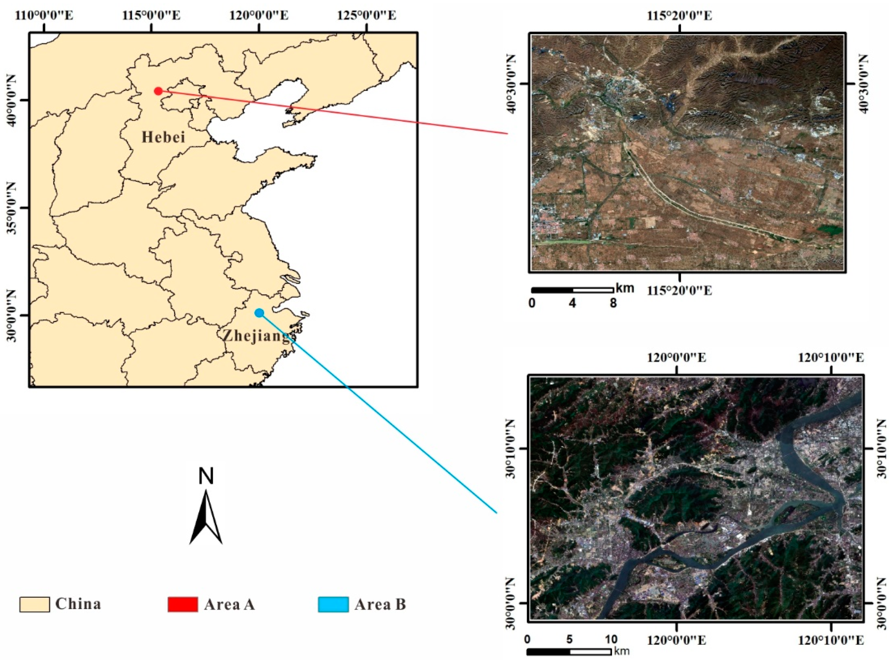
2.1. Study Area
2.1.1. Samples of Different Vegetation Species
2.1.2. Large Scale Study Area
2.2. Data
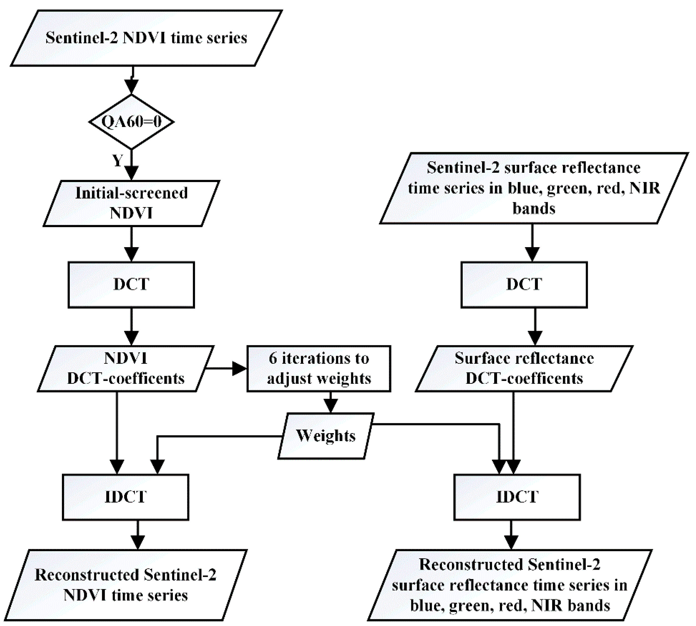
3. Methodology
3.1. Introduction of Original DCT-PLS Method
3.2. Reconfigure of the DCT-PLS for Irregular Interval Data
3.3. The Setting of N and s Parameters
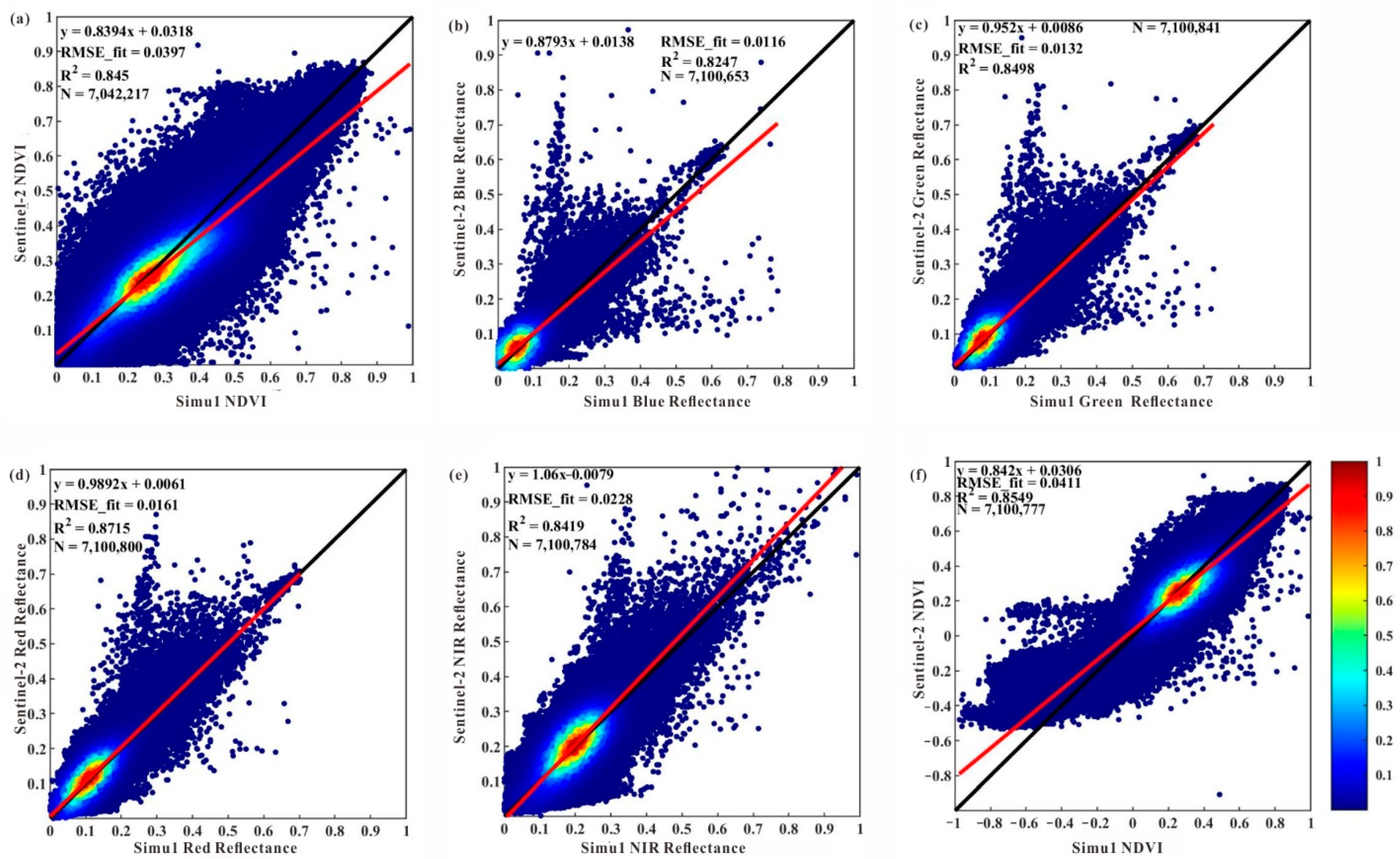
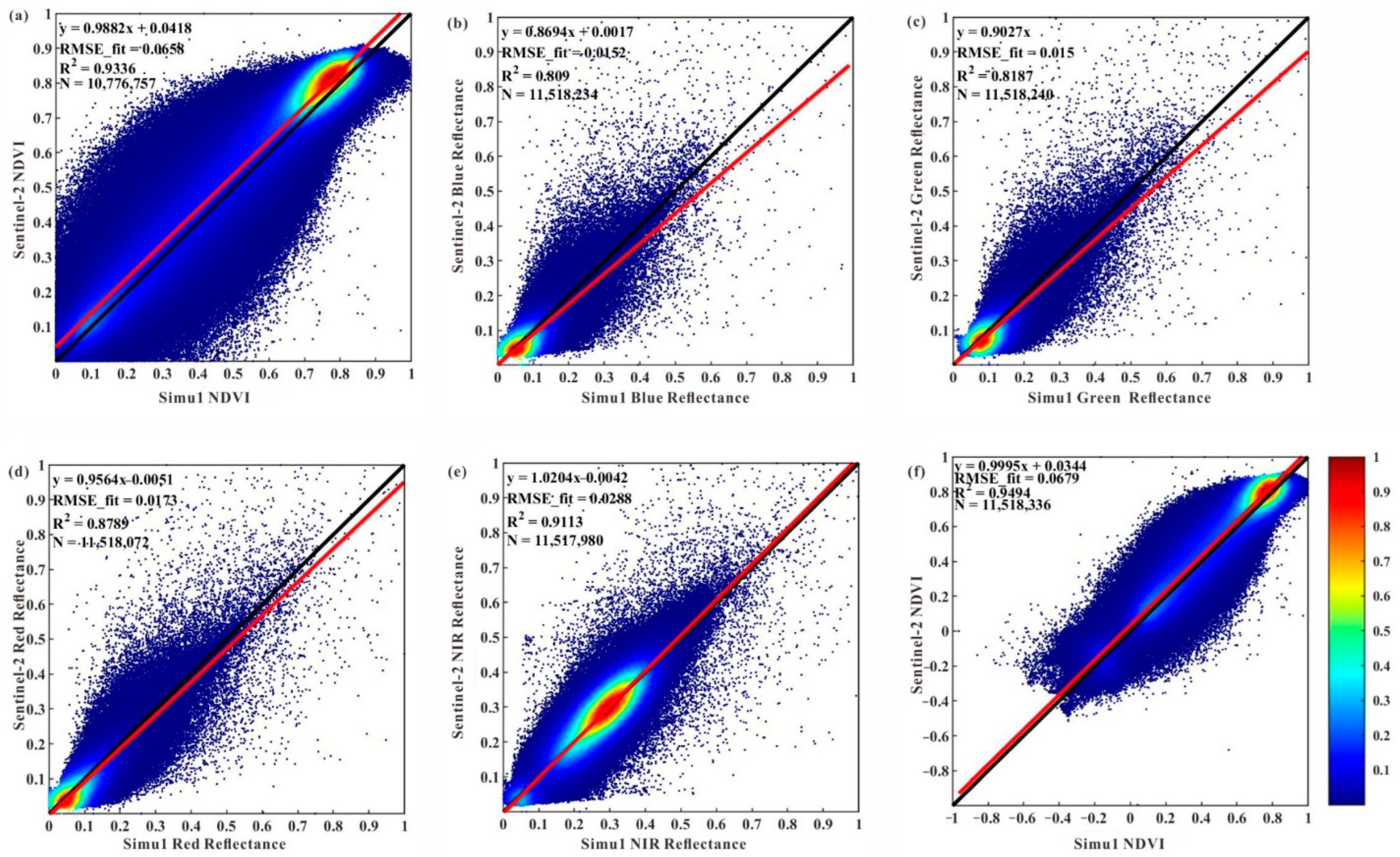
3.4. Relationship between the NDVI Reconstruction and Surface Reflectance Reconstruction
4. Results
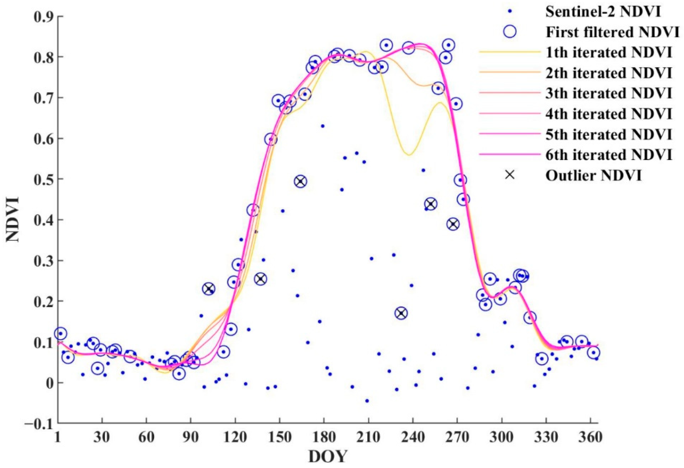
4.1. The Performance of Removing Outliers through Iterations
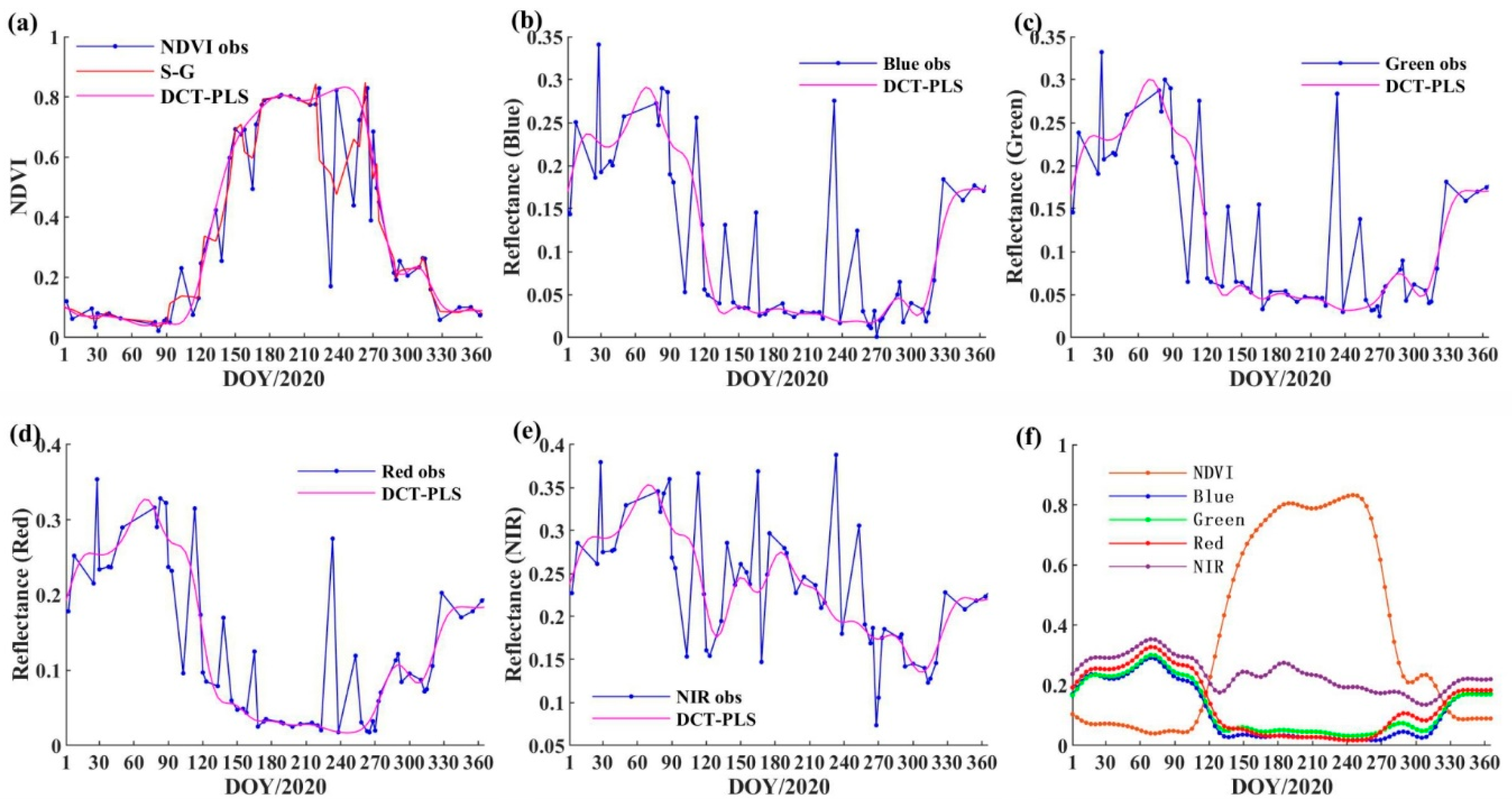
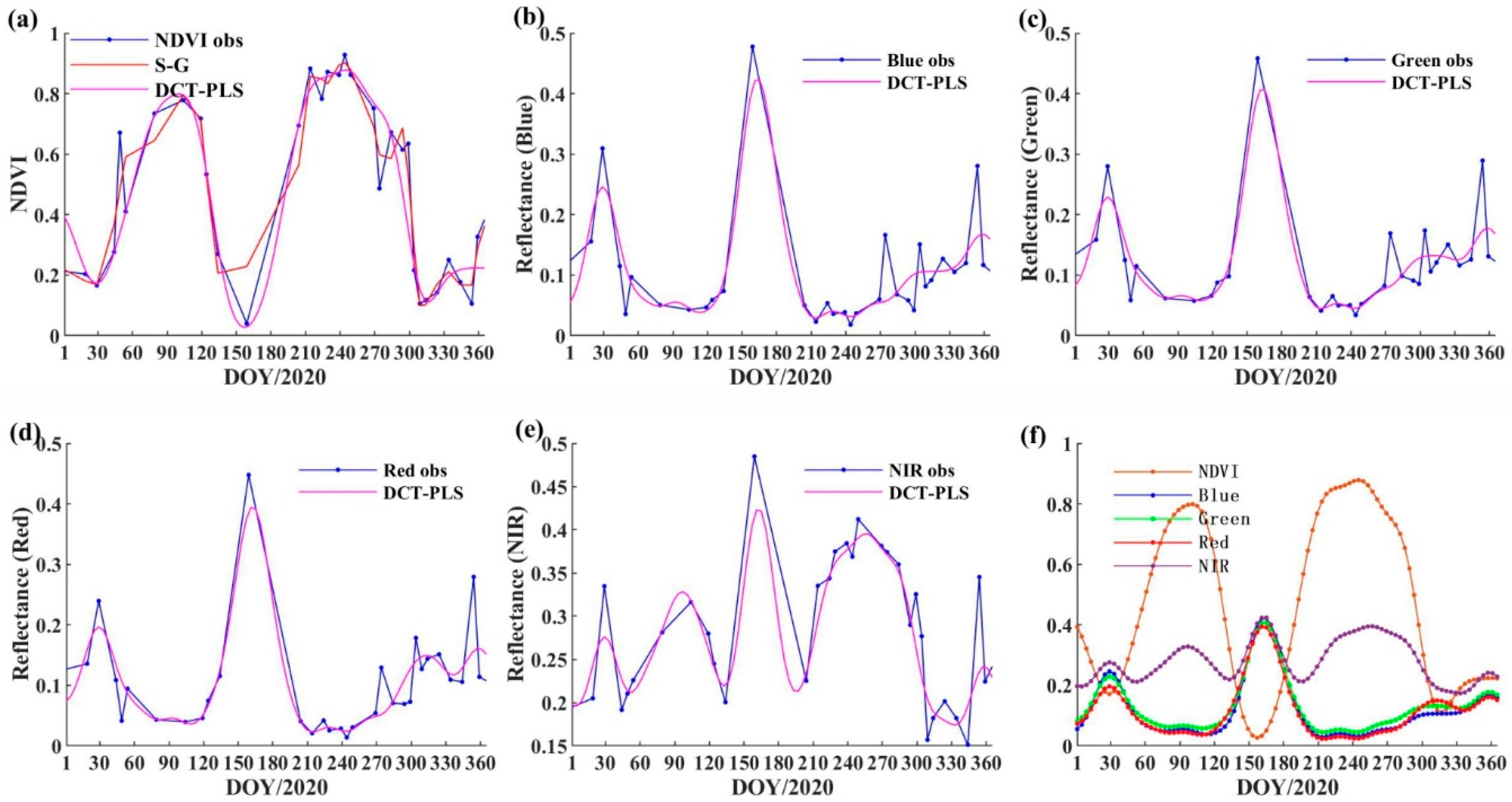
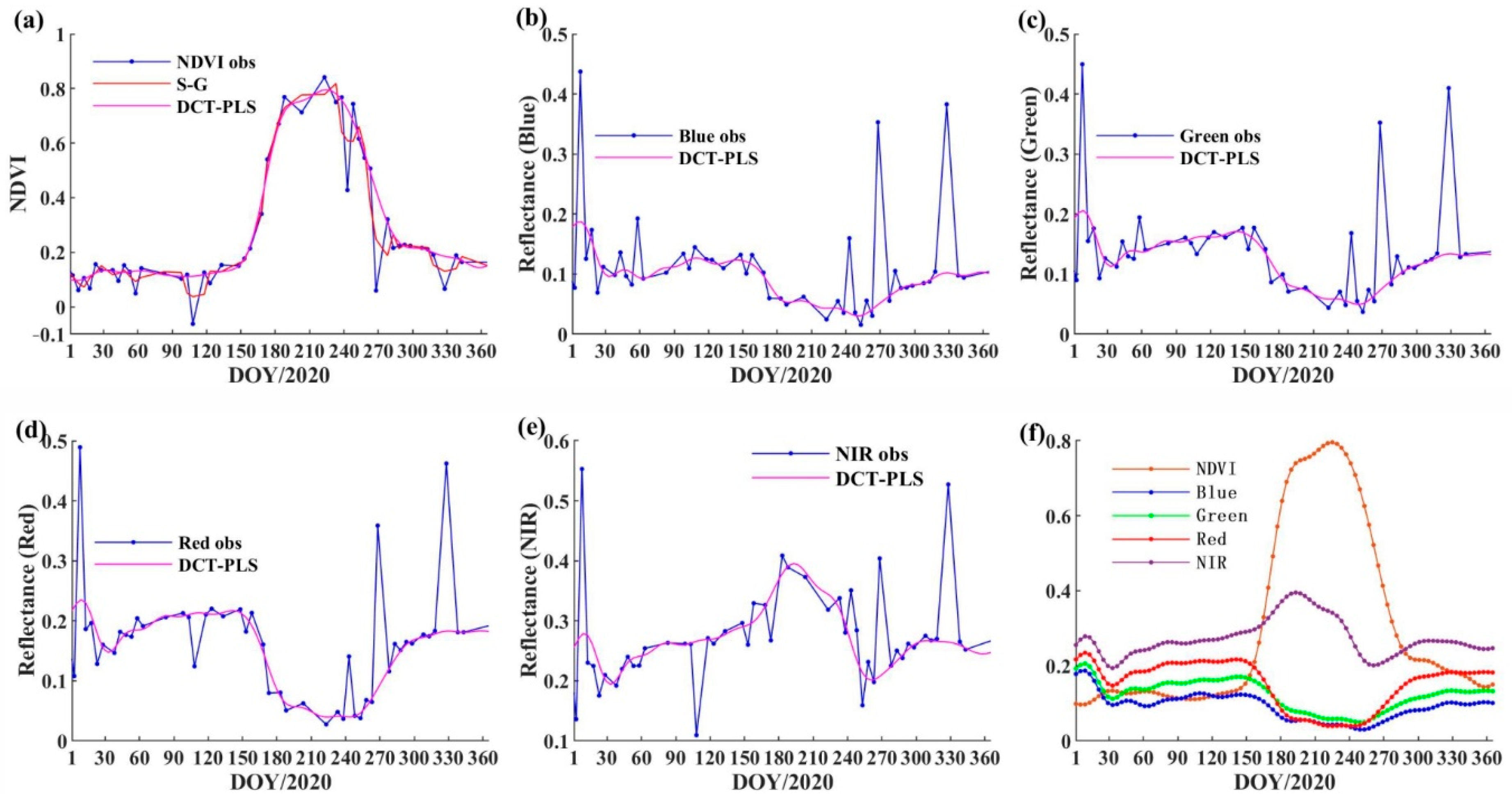
4.2. The Performance of Time Series Reconstruction on Typical Samples
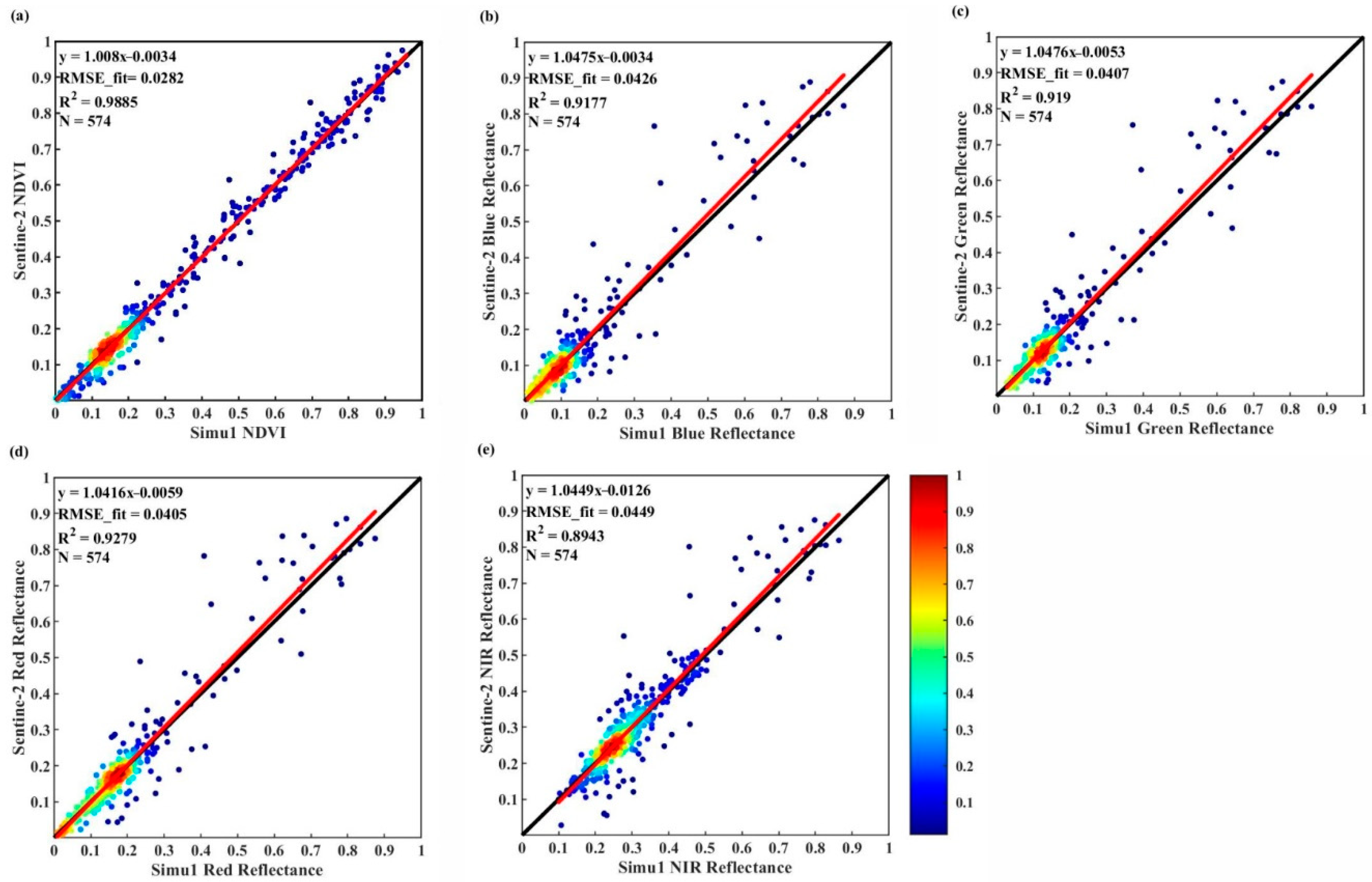
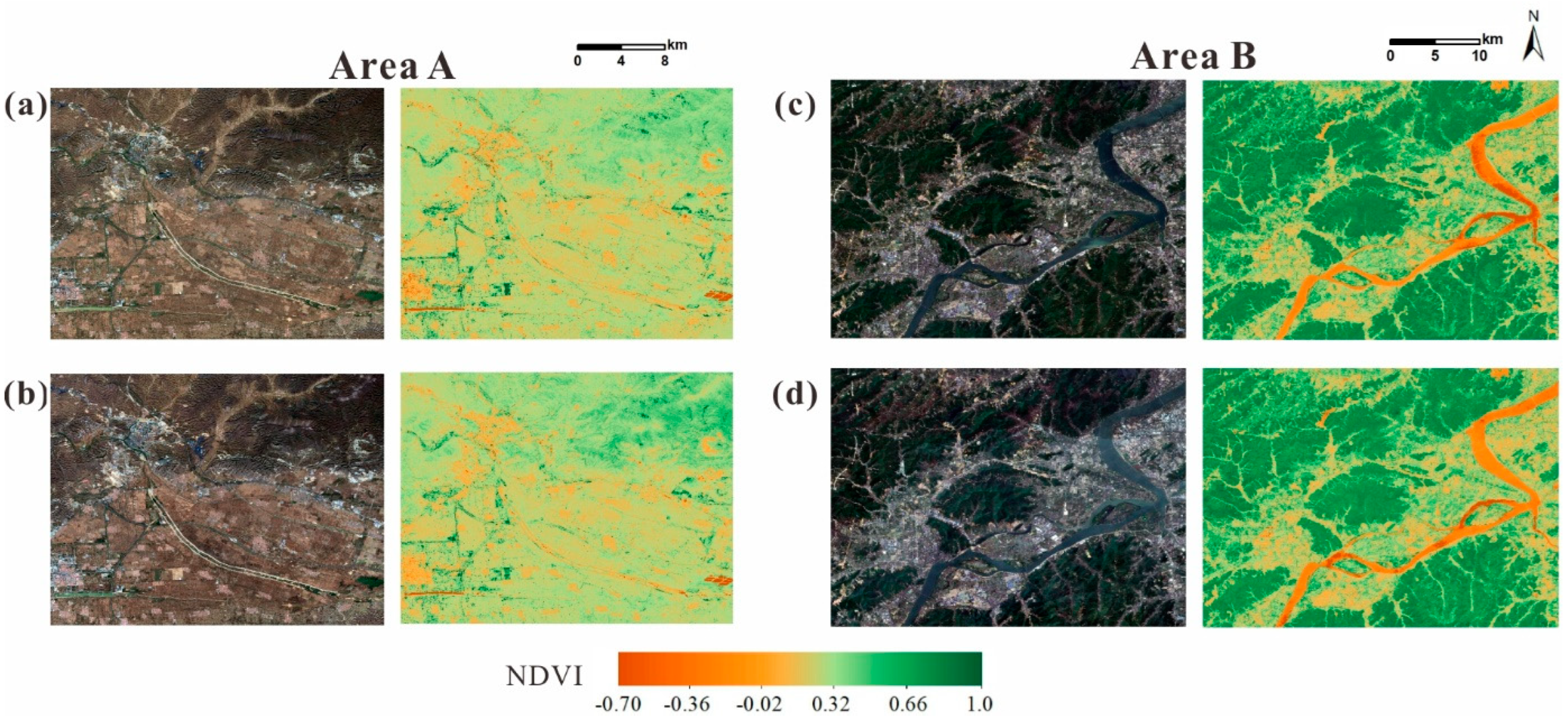
4.3. The Performance of Time Series Reconstruction for Images
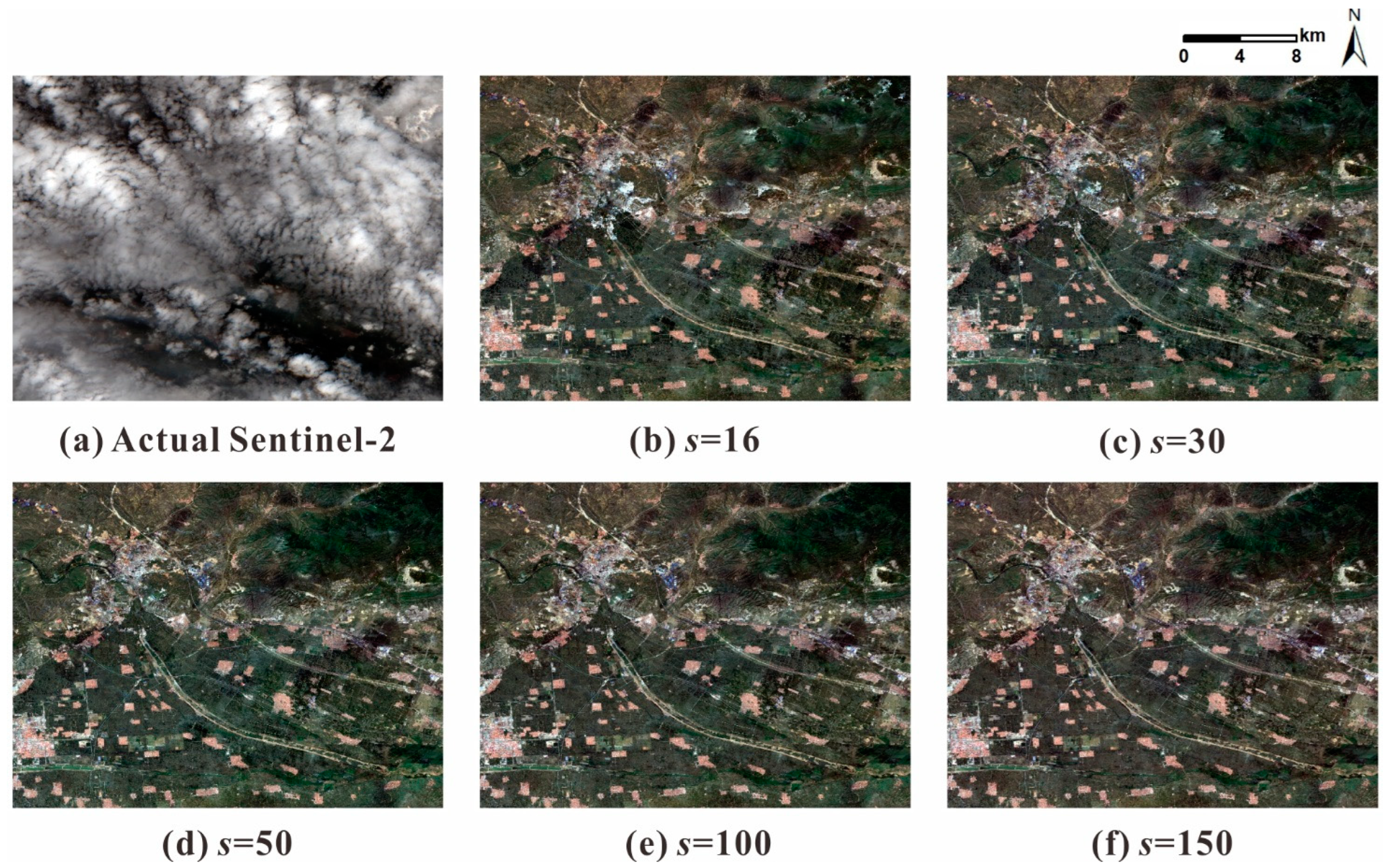
4.3.1. Case 1
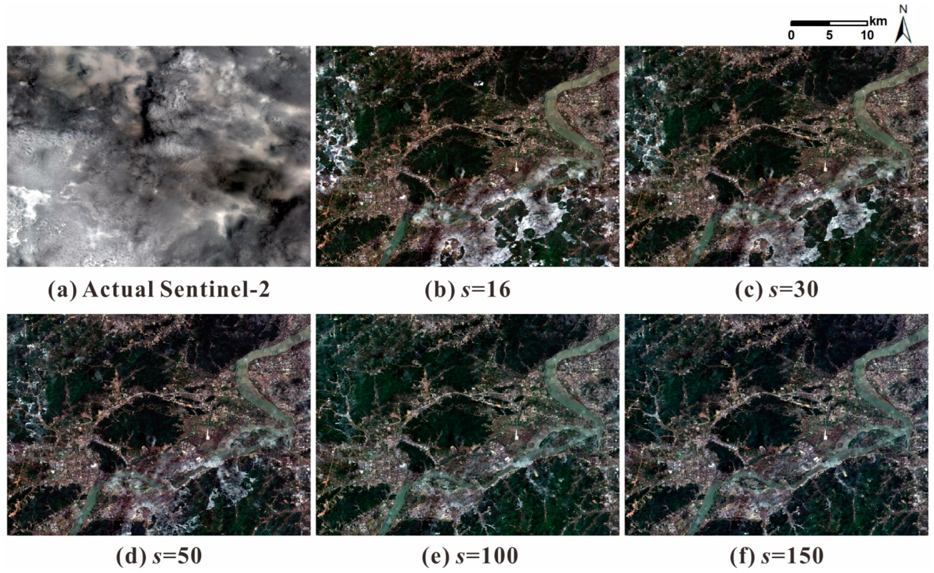
4.3.2. Case 2
4.3.3. Case 3
5. Conclusions
Supplementary Materials
Author Contributions
Funding
Data Availability Statement
Acknowledgments
Conflicts of Interest
References
- Liang, S.L.; Fang, H.L.; Chen, M.Z. Atmospheric Correction of Landsat Etm+ Land Surface Imagery-Part I: Methods. IEEE Trans. Geosci. Remote Sens. 2001, 39, 2490–2498. [Google Scholar] [CrossRef]
- Huang, S.; Tang, L.N.; Hupy, J.P.; Wang, Y.; Shao, G.F. A Commentary Review on the Use of Normalized Difference Vegetation Index (NDVI) in the Era of Popular Remote Sensing. J. For. Res. 2021, 32, 1–6. [Google Scholar] [CrossRef]
- Li, S.; Xu, L.; Jing, Y.H.; Yin, H.; Li, X.H.; Guan, X.B. High-Quality Vegetation Index Product Generation: A Review of NDVI Time Series Reconstruction Techniques. Int. J. Appl. Earth Obs. Geoinf. 2021, 105, 18. [Google Scholar] [CrossRef]
- Xie, Y.; Huang, J.X. Integration of a Crop Growth Model and Deep Learning Methods to Improve Satellite-Based Yield Estimation of Winter Wheat in Henan Province, China. Remote Sensing 2021, 13, 4372. [Google Scholar] [CrossRef]
- Sun, Y.H.; Ren, H.Z.; Zhang, T.Y.; Zhang, C.Y.; Qin, Q.M. Crop Leaf Area Index Retrieval Based on Inverted Difference Vegetation Index and NDVI. IEEE Geosci. Remote Sens. Lett. 2018, 15, 1662–1666. [Google Scholar] [CrossRef]
- Xiao, Z.; Liang, S.; Wang, T.; Liu, Q. Reconstruction of Satellite-Retrieved Land-Surface Reflectance Based on Temporally-Continuous Vegetation Indices. Remote Sens. 2015, 7, 9844–9864. [Google Scholar] [CrossRef]
- Zhou, F.Q.; Zhong, D.T.; Peiman, R. Reconstruction of Cloud-Free Sentinel-2 Image Time-Series Using an Extended Spatiotemporal Image Fusion Approach. Remote Sens. 2020, 12, 22. [Google Scholar] [CrossRef]
- Sun, L.; Gao, F.; Xie, D.; Anderson, M.; Chen, R.; Yang, Y.; Yang, Y.; Chen, Z. Reconstructing Daily 30 m NDVI over Complex Agricultural Landscapes Using a Crop Reference Curve Approach. Remote Sens. Environ. 2021, 253, 112156. [Google Scholar] [CrossRef]
- Chen, Y.; Cao, R.; Chen, J.; Liu, L.; Matsushita, B. A Practical Approach to Reconstruct High-Quality Landsat NDVI Time-Series Data by Gap Filling and the Savitzky–Golay Filter. ISPRS J. Photogramm. Remote Sens. 2021, 180, 174–190. [Google Scholar] [CrossRef]
- Drusch, M.; Del Bello, U.; Carlier, S.; Colin, O.; Fernandez, V.; Gascon, F.; Hoersch, B.; Isola, C.; Laberinti, P.; Martimort, P.; et al. Sentinel-2: Esa’s Optical High-Resolution Mission for Gmes Operational Services. Remote Sens. Environ. 2012, 120, 25–36. [Google Scholar] [CrossRef]
- Hunt, M.L.; Blackburn, G.A.; Carrasco, L.; Redhead, J.W.; Rowland, C.S. High Resolution Wheat Yield Mapping Using Sentinel-2. Remote Sens. Environ. 2019, 233, 15. [Google Scholar] [CrossRef]
- Llorens, R.; Sobrino, J.A.; Fernandez, C.; Fernandez-Alonso, J.M.; Vega, J.A. A Methodology to Estimate Forest Fires Burned Areas and Burn Severity Degrees Using Sentinel-2 Data. Application to the October 2017 Fires in the Iberian Peninsula. Int. J. Appl. Earth Obs. Geoinf. 2021, 95, 102243. [Google Scholar] [CrossRef]
- Xiao, D.Y.; Niu, H.P.; Guo, F.C.; Zhao, S.X.; Fan, L.X. Monitoring Irrigation Dynamics in Paddy Fields Using Spatiotemporal Fusion of Sentinel-2 and MODIS. Agric. Water Manag. 2022, 263, 107409. [Google Scholar] [CrossRef]
- Shen, H.; Li, X.; Cheng, Q.; Zeng, C.; Yang, G.; Li, H.; Zhang, L. Missing Information Reconstruction of Remote Sensing Data: A Technical Review. IEEE Geosci. Remote Sens. Mag. 2015, 3, 61–85. [Google Scholar] [CrossRef]
- Tang, Z.P.; Amatulli, G.; Pellikka, P.K.E.; Heiskanen, J. Spectral Temporal Information for Missing Data Reconstruction (Stimdr) of Landsat Reflectance Time Series. Remote Sens. 2022, 14, 172. [Google Scholar] [CrossRef]
- Tang, H.; Yu, K.; Hagolle, O.; Jiang, K.; Geng, X.; Zhao, Y. A Cloud Detection Method Based on a Time Series of MODIS Surface Reflectance Images. Int. J. Digit. Earth 2013, 6, 157–171. [Google Scholar] [CrossRef]
- Pouliot, D.; Latifovic, R. Reconstruction of Landsat Time Series in the Presence of Irregular and Sparse Observations: Development and Assessment in North-Eastern Alberta, Canada. Remote Sens. Environ. 2018, 204, 979–996. [Google Scholar] [CrossRef]
- Li, X.H.; Shen, H.F.; Zhang, L.P.; Li, H.F. Sparse-Based Reconstruction of Missing Information in Remote Sensing Images from Spectral/Temporal Complementary Information. ISPRS J. Photogramm. Remote Sens. 2015, 106, 1–15. [Google Scholar] [CrossRef]
- Wu, W.; Ge, L.Q.; Luo, J.C.; Huan, R.H.; Yang, Y.P. A Spectral-Temporal Patch-Based Missing Area Reconstruction for Time-Series Images. Remote Sens. 2018, 10, 1560. [Google Scholar] [CrossRef]
- Malambo, L.; Heatwole, C.D. A Multitemporal Profile-Based Interpolation Method for Gap Filling Nonstationary Data. IEEE Trans. Geosci. Remote Sens. 2016, 54, 252–261. [Google Scholar] [CrossRef]
- Yan, L.; Roy, D.P. Large-Area Gap Filling of Landsat Reflectance Time Series by Spectral-Angle-Mapper Based Spatio-Temporal Similarity (Samsts). Remote Sens. 2018, 10, 609. [Google Scholar] [CrossRef]
- Zhu, X.L.; Chen, J.; Gao, F.; Chen, X.H.; Masek, J.G. An Enhanced Spatial and Temporal Adaptive Reflectance Fusion Model for Complex Heterogeneous Regions. Remote Sens. Environ. 2010, 114, 2610–2623. [Google Scholar] [CrossRef]
- Zhu, X.L.; Helmer, E.H.; Gao, F.; Liu, D.S.; Chen, J.; Lefsky, M.A. A Flexible Spatiotemporal Method for Fusing Satellite Images with Different Resolutions. Remote Sens. Environ. 2016, 172, 165–177. [Google Scholar] [CrossRef]
- Zhong, D.T.; Zhou, F.Q. A Prediction Smooth Method for Blending Landsat and Moderate Resolution Imagine Spectroradiometer Images. Remote Sens. 2018, 10, 1371. [Google Scholar] [CrossRef]
- Julien, Y.; Sobrino, J.A. Comparison of Cloud-Reconstruction Methods for Time Series of Composite NDVI Data. Remote Sens. Environ. 2010, 114, 618–625. [Google Scholar] [CrossRef]
- Roy, D.P.; Yan, L. Robust Landsat-Based Crop Time Series Modelling. Remote Sens. Environ. 2020, 238, 16. [Google Scholar] [CrossRef]
- Chen, J.; Jönsson, P.; Tamura, M.; Gu, Z.; Matsushita, B.; Eklundh, L. A Simple Method for Reconstructing a High-Quality NDVI Time-Series Data Set Based on the Savitzky–Golay Filter. Remote Sens. Environ. 2004, 91, 332–344. [Google Scholar] [CrossRef]
- Ma, M.; Veroustraete, F. Reconstructing Pathfinder Avhrr Land NDVI Time-Series Data for the Northwest of China. Adv. Space Res. 2006, 37, 835–840. [Google Scholar] [CrossRef]
- Zhu, W.Q.; Pan, Y.Z.; He, H.; Wang, L.L.; Mou, M.J.; Liu, J.H. A Changing-Weight Filter Method for Reconstructing a High-Quality NDVI Time Series to Preserve the Integrity of Vegetation Phenology. IEEE Trans. Geosci. Remote Sens. 2012, 50, 1085–1094. [Google Scholar] [CrossRef]
- Jonsson, P.; Eklundh, L. Seasonality Extraction by Function Fitting to Time-Series of Satellite Sensor Data. IEEE Trans. Geosci. Remote Sens. 2002, 40, 1824–1832. [Google Scholar] [CrossRef]
- Beck, P.S.A.; Atzberger, C.; Hogda, K.A.; Johansen, B.; Skidmore, A.K. Improved Monitoring of Vegetation Dynamics at Very High Latitudes: A New Method Using MODIS NDVI. Remote Sens. Environ. 2006, 100, 321–334. [Google Scholar] [CrossRef]
- Das, M.; Ghosh, S.K. A Deep-Learning-Based Forecasting Ensemble to Predict Missing Data for Remote Sensing Analysis. IEEE J. Sel. Top. Appl. Earth Obs. Remote Sens. 2017, 10, 5228–5236. [Google Scholar] [CrossRef]
- Ahmad, R.; Yang, B.; Ettlin, G.; Berger, A.; Rodriguez-Bocca, P. A Machine-Learning Based Convlstm Architecture for NDVI Forecasting. Int. Trans. Oper. Res. 2020, 28, 12887. [Google Scholar] [CrossRef]
- Roerink, G.J.; Menenti, M.; Verhoef, W. Reconstructing Cloudfree NDVI Composites Using Fourier Analysis of Time Series. Int. J. Remote Sens. 2000, 21, 1911–1917. [Google Scholar] [CrossRef]
- Lu, X.L.; Liu, R.G.; Liu, J.Y.; Liang, S.L. Removal of Noise by Wavelet Method to Generate High Quality Temporal Data of Terrestrial MODIS Products. Photogramm. Eng. Remote Sens. 2007, 73, 1129–1139. [Google Scholar] [CrossRef]
- Cao, R.Y.; Chen, Y.; Shen, M.G.; Chen, J.; Zhou, J.; Wang, C.; Yang, W. A Simple Method to Improve the Quality of NDVI Time-Series Data by Integrating Spatiotemporal Information with the Savitzky-Golay Filter. Remote Sens. Environ. 2018, 217, 244–257. [Google Scholar] [CrossRef]
- Padhee, S.K.; Dutta, S. Spatio-Temporal Reconstruction of MODIS NDVI by Regional Land Surface Phenology and Harmonic Analysis of Time-Series. GISci. Remote Sens. 2019, 56, 1261–1288. [Google Scholar] [CrossRef]
- Chu, D.; Shen, H.F.; Guan, X.B.; Chen, J.M.; Li, X.H.; Li, J.; Zhang, L.P. Long Time-Series NDVI Reconstruction in Cloud-Prone Regions Via Spatio-Temporal Tensor Completion. Remote Sens. Environ. 2021, 264, 112632. [Google Scholar] [CrossRef]
- Wang, Q.M.; Atkinson, P.M. Spatio-Temporal Fusion for Daily Sentinel-2 Images. Remote Sens. Environ. 2018, 204, 31–42. [Google Scholar] [CrossRef]
- Xiong, S.P.; Du, S.H.; Zhang, X.Y.; Ouyang, S.; Cui, W.H. Fusing Landsat-7, Landsat-8 and Sentinel-2 Surface Reflectance to Generate Dense Time Series Images with 10m Spatial Resolution. Int. J. Remote Sens. 2022, 43, 1630–1654. [Google Scholar] [CrossRef]
- Gorelick, N.; Hancher, M.; Dixon, M.; Ilyushchenko, S.; Thau, D.; Moore, R. Google Earth Engine: Planetary-Scale Geospatial Analysis for Everyone. Remote Sens. Environ. 2017, 202, 18–27. [Google Scholar] [CrossRef]
- Kong, D.; Zhang, Y.; Gu, X.; Wang, D. A Robust Method for Reconstructing Global MODIS Evi Time Series on the Google Earth Engine. ISPRS J. Photogramm. Remote Sens. 2019, 155, 13–24. [Google Scholar] [CrossRef]
- Khanal, N.; Matin, M.A.; Uddin, K.; Poortinga, A.; Chishtie, F.; Tenneson, K.; Saah, D. A Comparison of Three Temporal Smoothing Algorithms to Improve Land Cover Classification: A Case Study from Nepal. Remote Sens. 2020, 12, 2888. [Google Scholar] [CrossRef]
- Liu, X.K.; Ji, L.Y.; Zhang, C.; Liu, Y.H. A Method for Reconstructing NDVI Time-Series Based on Envelope Detection and the Savitzky-Golay Filter. Int. J. Digit. Earth 2022, 15, 553–584. [Google Scholar] [CrossRef]
- Garcia, D. Robust Smoothing of Gridded Data in One and Higher Dimensions with Missing Values. Comput. Stat. Data Anal. 2010, 54, 1167–1178. [Google Scholar] [CrossRef]
- Rousseeuw, P.J.; Leroy, A.M. Robust Regression and Outlier Detection; John Wiley & Sons: New York, NY, USA, 1987. [Google Scholar]
- Savitzky, A.; Golay, M.J.E. Smoothing + Differentiation of Data by Simplified Least Squares Procedures. Anal. Chem. 1964, 36, 1627–1639. [Google Scholar] [CrossRef]


| Typical Vegetation Samples | Sample ID | Province | Longitude (°E) | Latitude (°N) |
|---|---|---|---|---|
| Larch | 1 | Hebei | 117.50 | 42.58 |
| Rotation of rice | 2 | Zhejiang | 120.47 | 30.37 |
| Rice | 3 | Liaoning | 122.09 | 40.99 |
| Rotation of wheat and corn | 4 | Henan | 113.78 | 33.92 |
| Grass | 5 | Hebei | 114.76 | 41.29 |
| Soybean | 6 | Hebei | 114.79 | 41.18 |
| Potato | 7 | Hebei | 114.92 | 41.35 |
| Grape | 8 | Hebei | 115.43 | 40.34 |
| Tobacco | 9 | Hebei | 114.66 | 39.81 |
| Corn | 10 | Hebei | 115.31 | 40.37 |
| Sentinel-2 L2A Product Information in the Selected Bands | ||||
|---|---|---|---|---|
| Band Name | Description | Central Wavelength (nm) | Bandwidth (nm) | Resolution (m) |
| B2 | Blue | 490 | 65 | 10 |
| B3 | Green | 560 | 35 | 10 |
| B4 | Red | 665 | 30 | 10 |
| B8 | NIR | 842 | 115 | 10 |
| QA60 | Cloud mask | - | - | 60 |
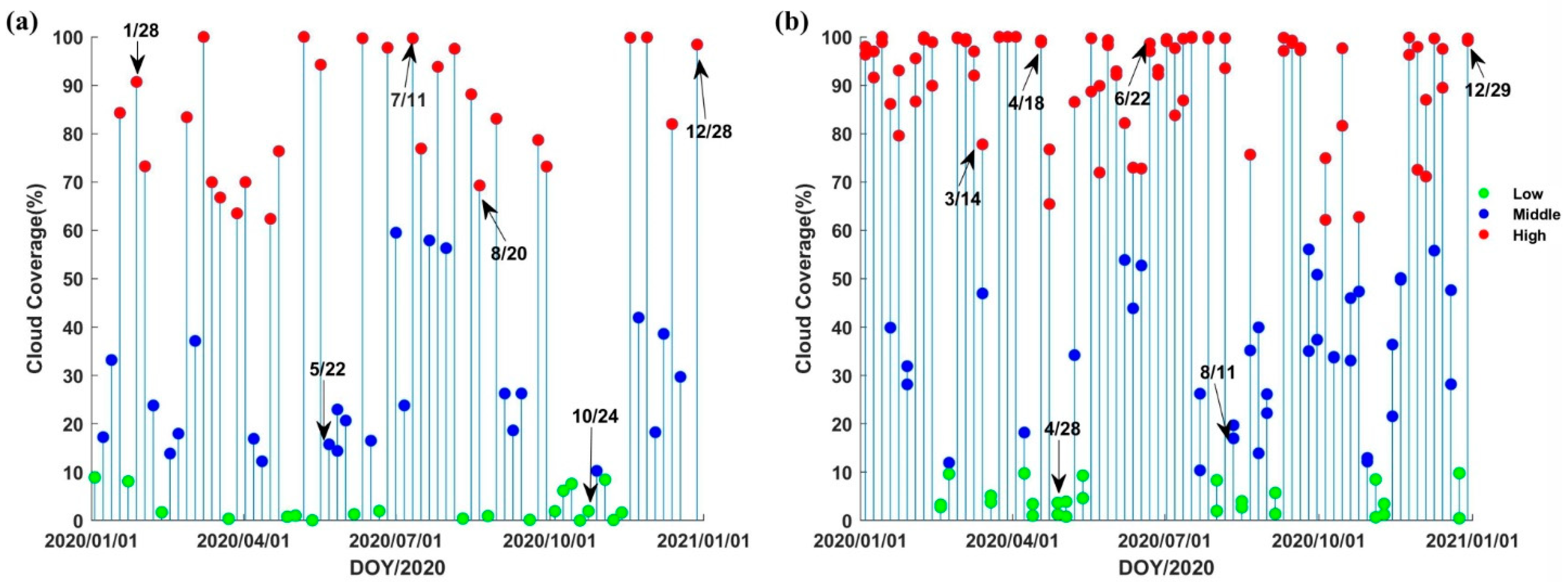
| Information of available images in the two study areas | ||||
| Study Area | Date range | Number (used/total) | Average cloud coverage (used/total) | |
| Area A | 1 June 2019–1 June 2021 | 117/149 | 25.74%/40.28% | |
| Area B | 1 June 2019–1 June 2021 | 162/301 | 28.50%/59.61% | |
| N | 12 | 24 | 36 | 48 | |||||
|---|---|---|---|---|---|---|---|---|---|
| Vegetation Samples | RMSE_cv | R2 | RMSE_cv | R2 | RMSE_cv | R2 | RMSE_cv | R2 | |
| Larch | 0.0601 | 0.9594 | 0.0487 | 0.9750 | 0.0463 | 0.9774 | 0.0489 | 0.9746 | |
| Rotation of rice | 0.1121 | 0.8561 | 0.0843 | 0.9268 | 0.0941 | 0.9102 | 0.1203 | 0.8708 | |
| Rice | 0.0472 | 0.9667 | 0.0402 | 0.9760 | 0.0370 | 0.9800 | 0.0307 | 0.9865 | |
| Rotation of wheat and corn | 0.0597 | 0.9569 | 0.0486 | 0.9715 | 0.0354 | 0.9855 | 0.0210 | 0.9949 | |
| Grass | 0.0341 | 0.9619 | 0.0220 | 0.9841 | 0.0235 | 0.9824 | 0.0212 | 0.9857 | |
| Soybean | 0.0405 | 0.9544 | 0.0329 | 0.9724 | 0.0325 | 0.9719 | 0.0339 | 0.9687 | |
| Potato | 0.0318 | 0.9822 | 0.0216 | 0.9919 | 0.0200 | 0.9930 | 0.0258 | 0.9901 | |
| Grape | 0.0399 | 0.9638 | 0.0259 | 0.9846 | 0.0375 | 0.9679 | 0.0407 | 0.9624 | |
| Tobacco | 0.0296 | 0.9807 | 0.0225 | 0.9889 | 0.0224 | 0.9890 | 0.0224 | 0.9890 | |
| Corn | 0.0410 | 0.9692 | 0.0483 | 0.9596 | 0.0522 | 0.9532 | 0.0571 | 0.9444 | |
| Mean | 0.0496 | 0.9551 | 0.0395 | 0.9731 | 0.0401 | 0.9710 | 0.0422 | 0.9667 | |
| Typical Vegetation Samples | RMSE_cv-mi | _opt | The Acceptable Range of |
|---|---|---|---|
| Larch | 0.0487 | 16 | 8–48 |
| Rotation of rice | 0.0843 | 22 | 13–59 |
| Rice | 0.0402 | 43 | 0.1–60 |
| Rotation of wheat and corn | 0.0486 | 5 | 2–22 |
| Grass | 0.0220 | 14 | 0.1–57 |
| Soybean | 0.0329 | 16 | 0.1–60 |
| Potato | 0.0216 | 6 | 0.1–20 |
| Grape | 0.0259 | 18 | 6–60 |
| Tobacco | 0.0225 | 16 | 0.1–52 |
| Corn | 0.0483 | 45 | 13–60 |
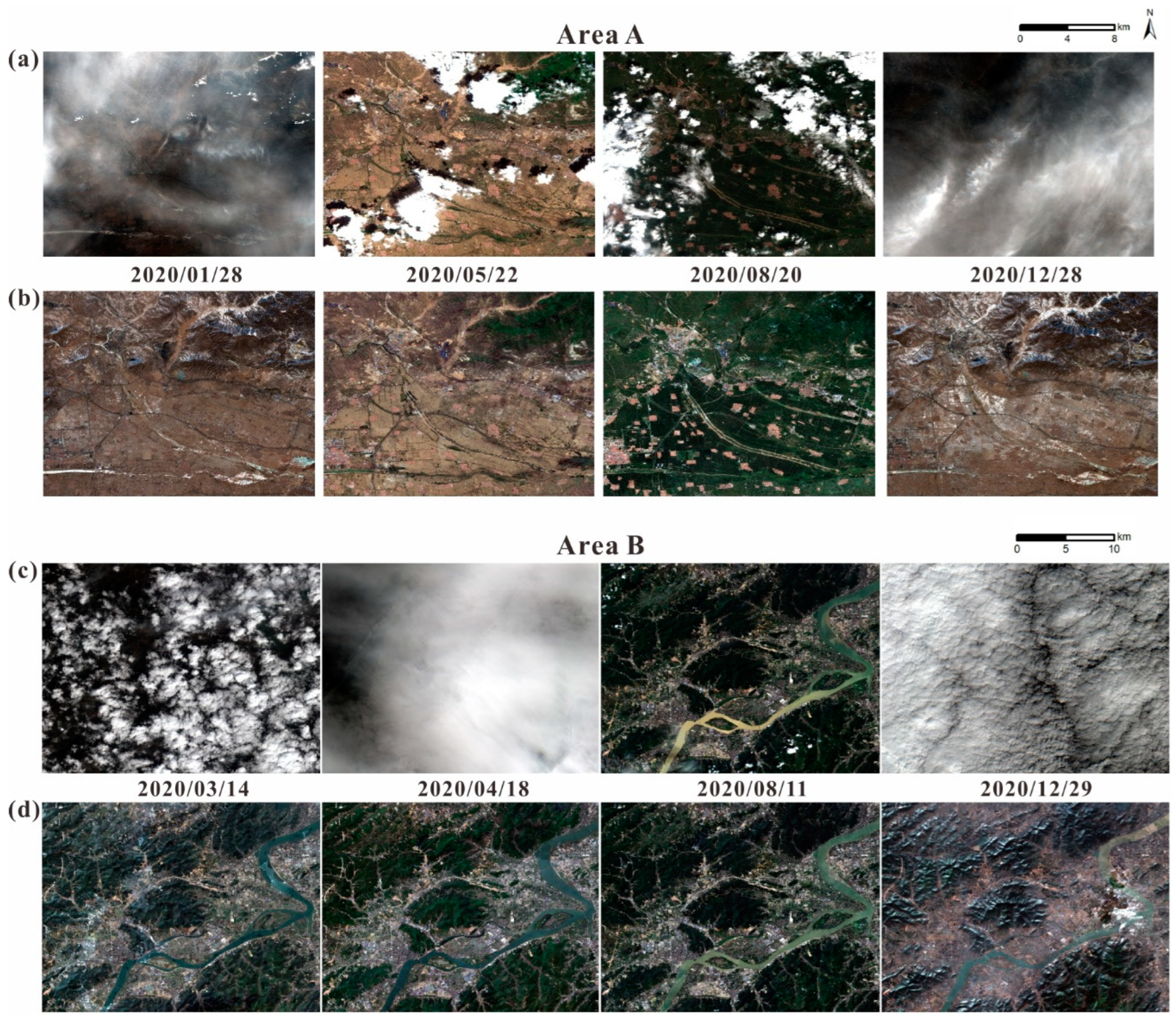
| Case | Area A | Area B |
|---|---|---|
| Case1 | 10–24 | 4–28 |
| Case2 | 1–28, 5–22, 8–20, 12–28 | 3–14, 4–18, 8–11,12–29 |
| Case3 | 7–11 | 6–22 |
Publisher’s Note: MDPI stays neutral with regard to jurisdictional claims in published maps and institutional affiliations. |
© 2022 by the authors. Licensee MDPI, Basel, Switzerland. This article is an open access article distributed under the terms and conditions of the Creative Commons Attribution (CC BY) license (https://creativecommons.org/licenses/by/4.0/).
Share and Cite
Yang, K.; Luo, Y.; Li, M.; Zhong, S.; Liu, Q.; Li, X. Reconstruction of Sentinel-2 Image Time Series Using Google Earth Engine. Remote Sens. 2022, 14, 4395. https://doi.org/10.3390/rs14174395
Yang K, Luo Y, Li M, Zhong S, Liu Q, Li X. Reconstruction of Sentinel-2 Image Time Series Using Google Earth Engine. Remote Sensing. 2022; 14(17):4395. https://doi.org/10.3390/rs14174395
Chicago/Turabian StyleYang, Kaixiang, Youming Luo, Mengyao Li, Shouyi Zhong, Qiang Liu, and Xiuhong Li. 2022. "Reconstruction of Sentinel-2 Image Time Series Using Google Earth Engine" Remote Sensing 14, no. 17: 4395. https://doi.org/10.3390/rs14174395
APA StyleYang, K., Luo, Y., Li, M., Zhong, S., Liu, Q., & Li, X. (2022). Reconstruction of Sentinel-2 Image Time Series Using Google Earth Engine. Remote Sensing, 14(17), 4395. https://doi.org/10.3390/rs14174395