
Column-Spatial Correction Network for Remote Sensing Image Destriping


Abstract
:1. Introduction
- (1)
- Based on the structural characteristics of stripe, we propose a multi-scaled column-spatial correction network (CSCNet), aiming at improving the local consistency of homogeneous region and the global uniformity of whole image. The proposed CSCNet can effectively remove different kinds of stripe noise, including non-periodic, periodic, and wide stripe.
- (2)
- A column-based correction module is proposed to reduce the differences between columns caused by stripe noise. To the best of our knowledge, this was one of the first attempts to explore the column-based correction strategy in deep neural network-based models for destriping according to the structural characteristics of the stripe.
- (3)
- The proposed method has been evaluated on both simulated and real remote sensing images with promising results. Compared to existing methods, our CSCNet has achieved superior qualitative and quantitative assessments.
2. Related Work
2.1. Statistical-Based Methods
2.2. Filtering-Based Methods
2.3. Optimization-Based Methods
2.4. Deep Learning-Based Methods
3. Methodology
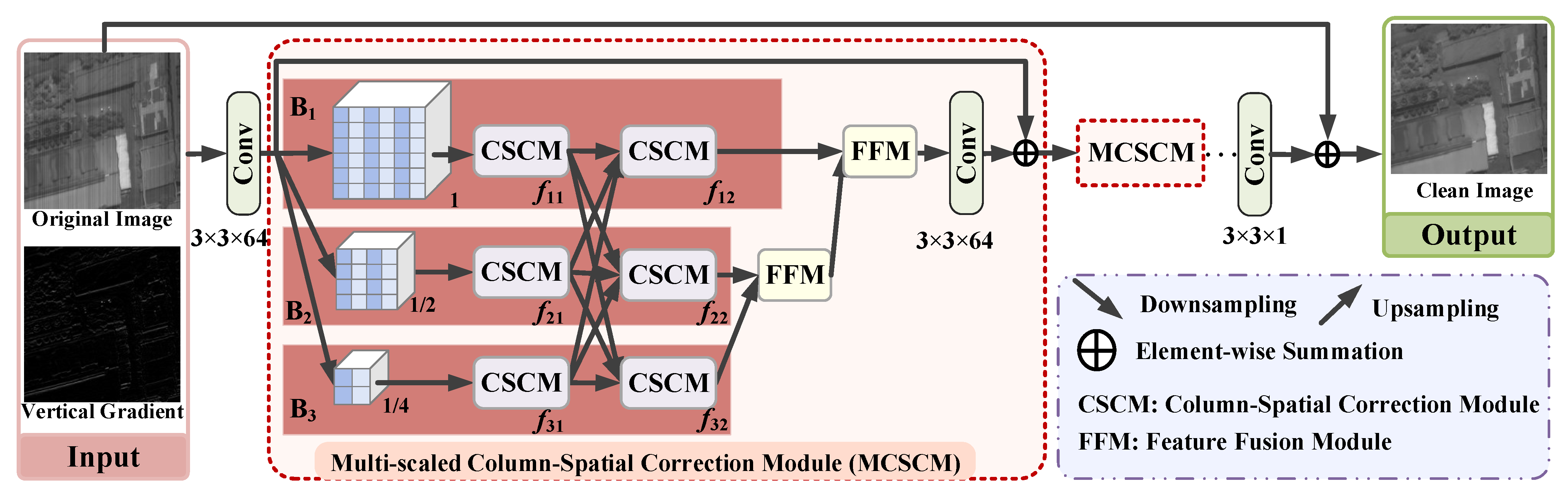
3.1. Overall Framework
3.2. Multi-Scaled Column-Spatial Correction Module
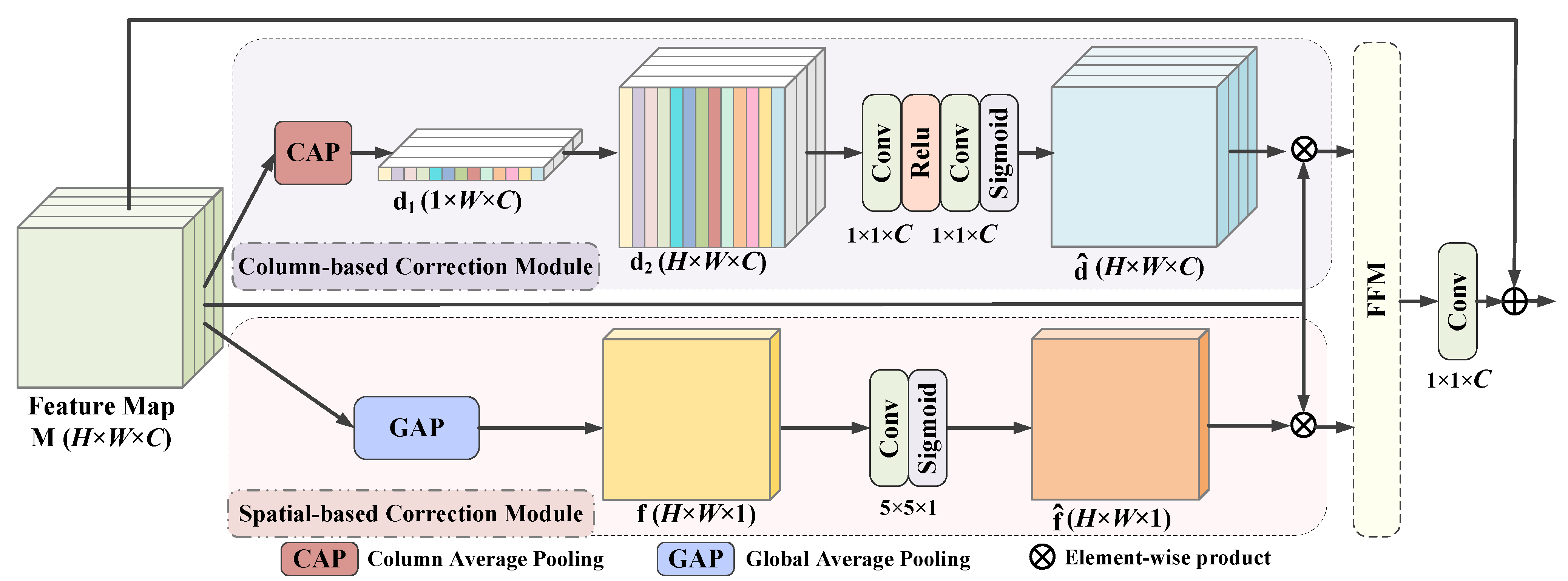
3.3. Column-Spatial Correction Module
3.3.1. Column-Based Correction Module
3.3.2. Spatial-Based Correction Module
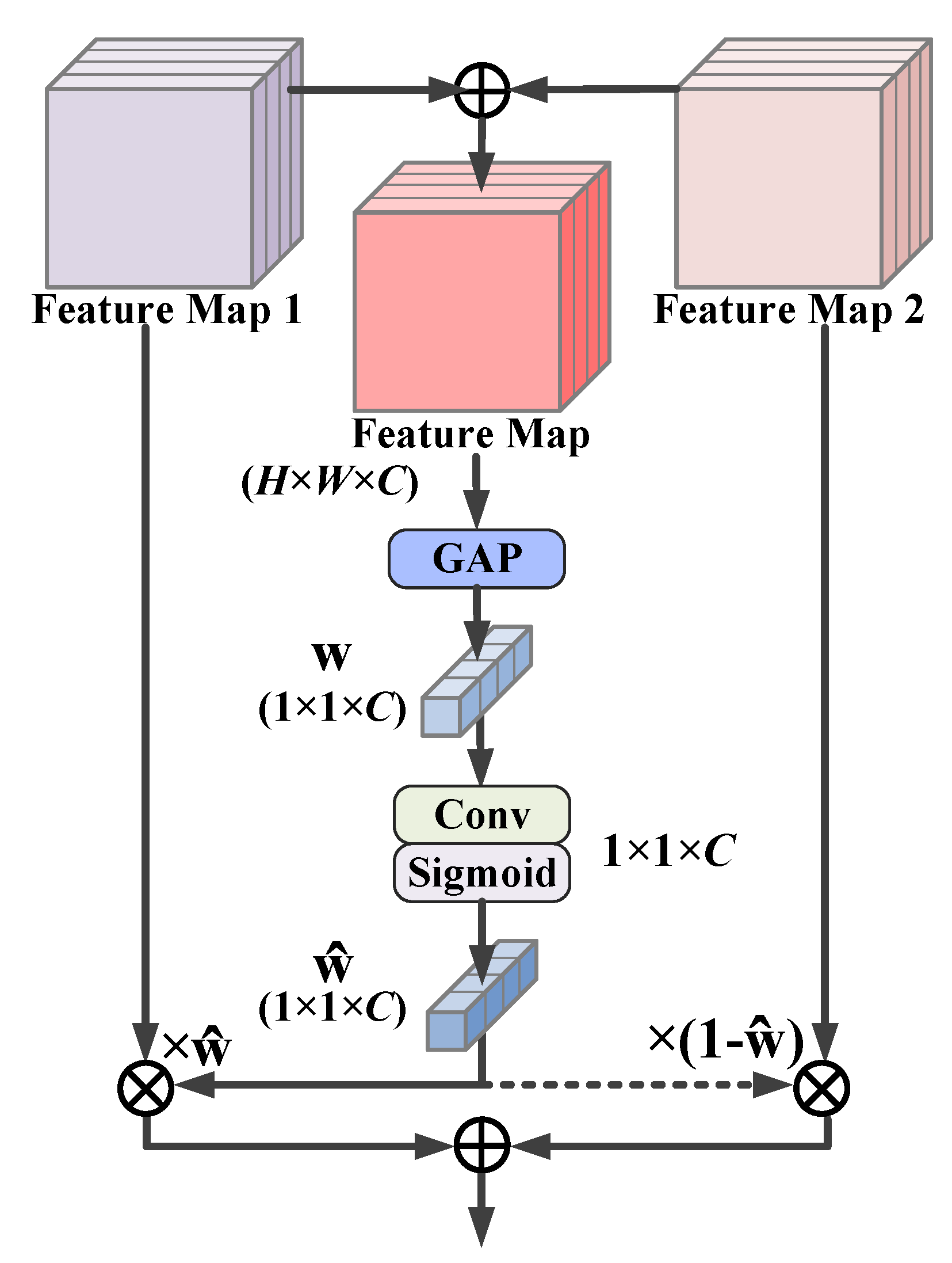
3.4. Feature Fusion Module
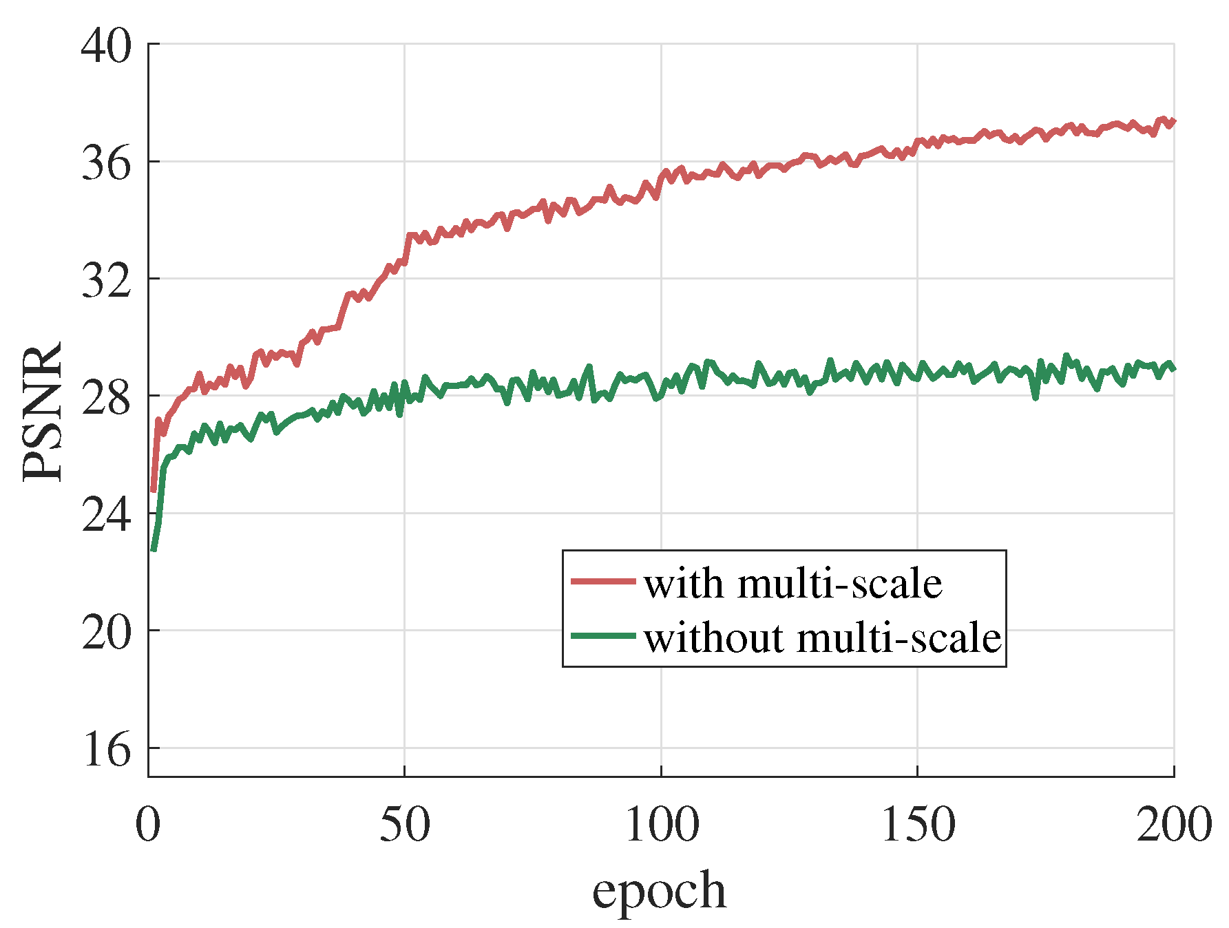
3.5. Multi-Scale Extension
3.6. Training Details
4. Experimental Results and Analysis
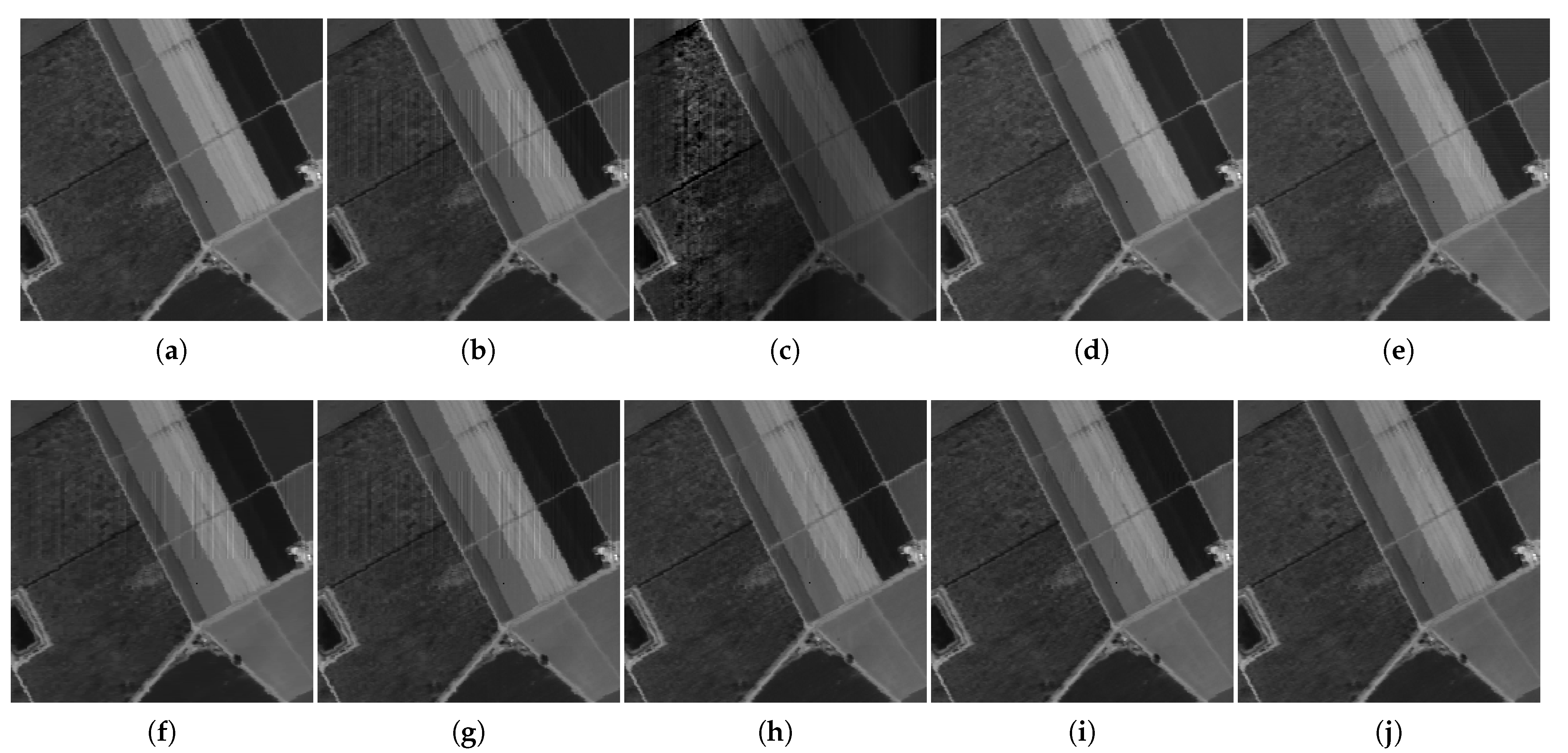
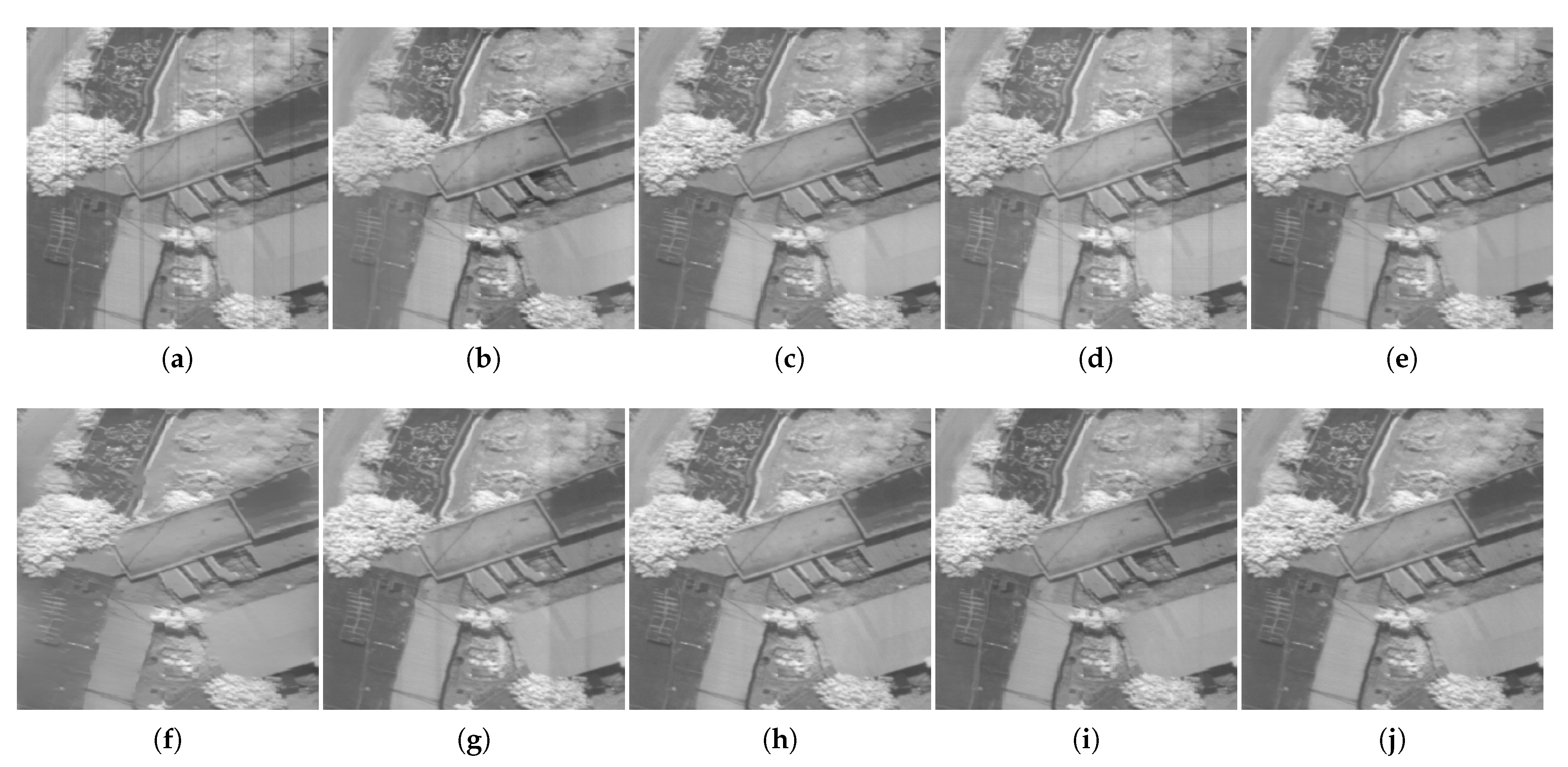
4.1. Simulated Image Destriping
4.1.1. Simulated Data Preparation
4.1.2. Evaluation
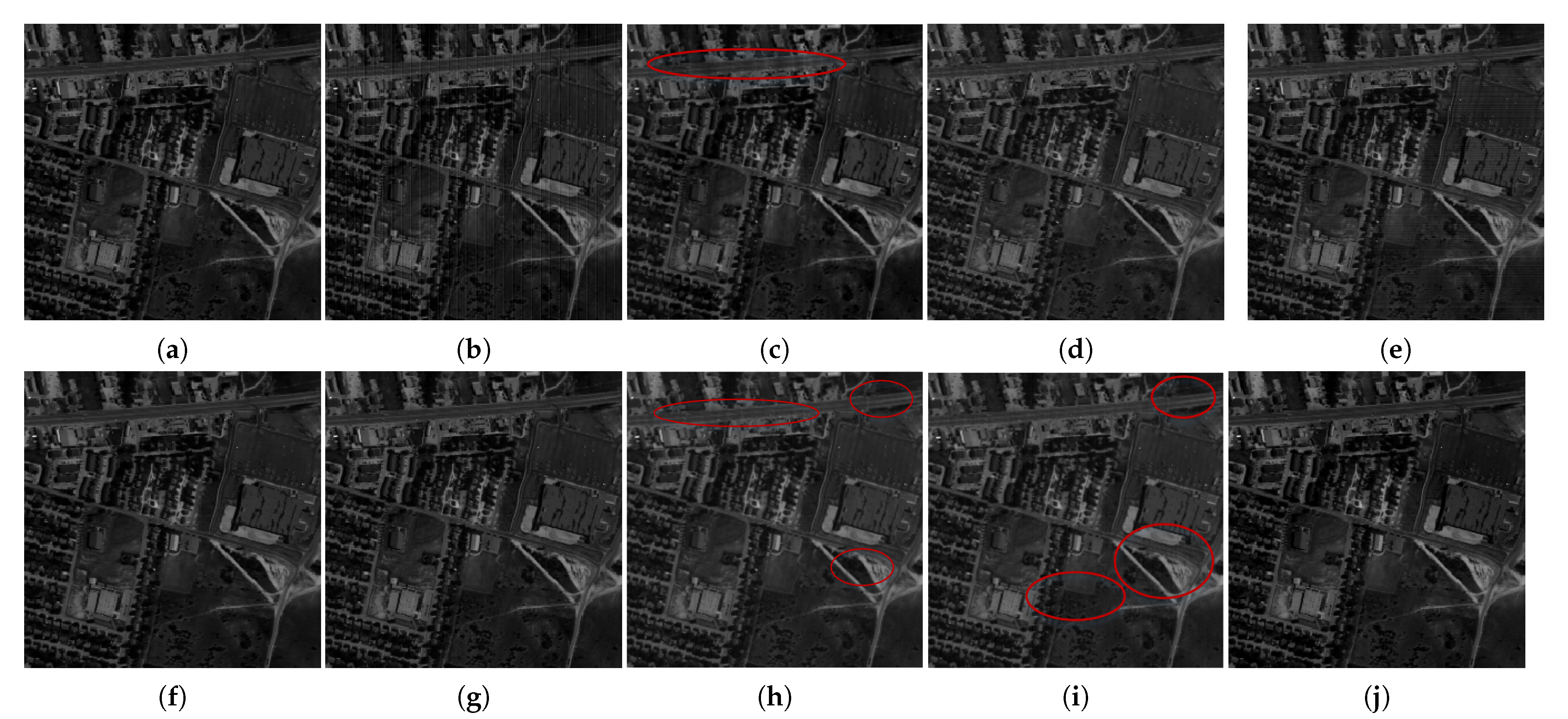
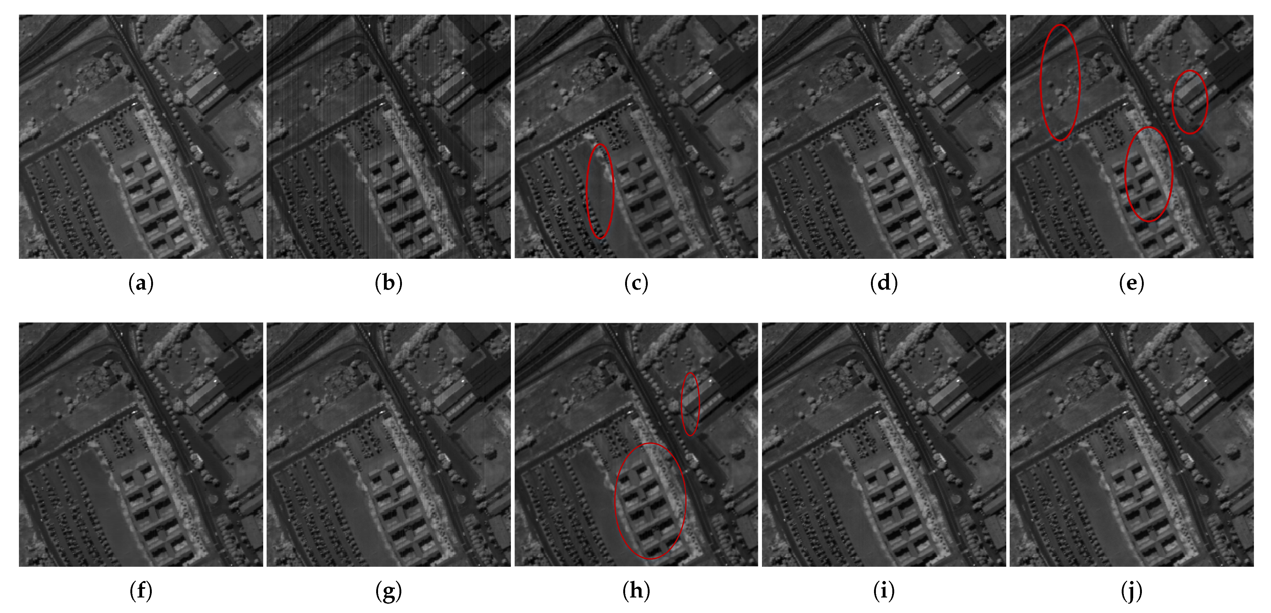
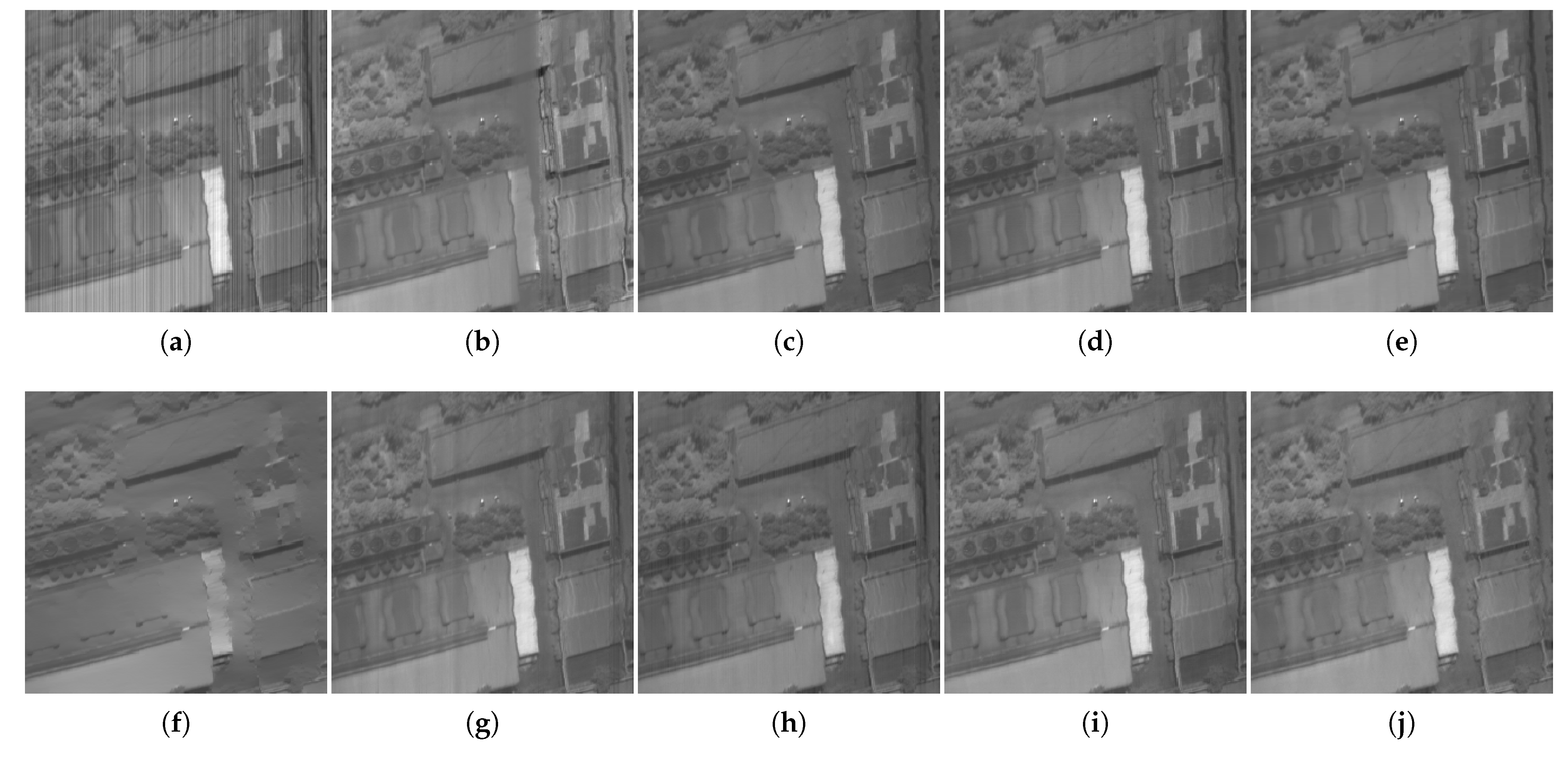
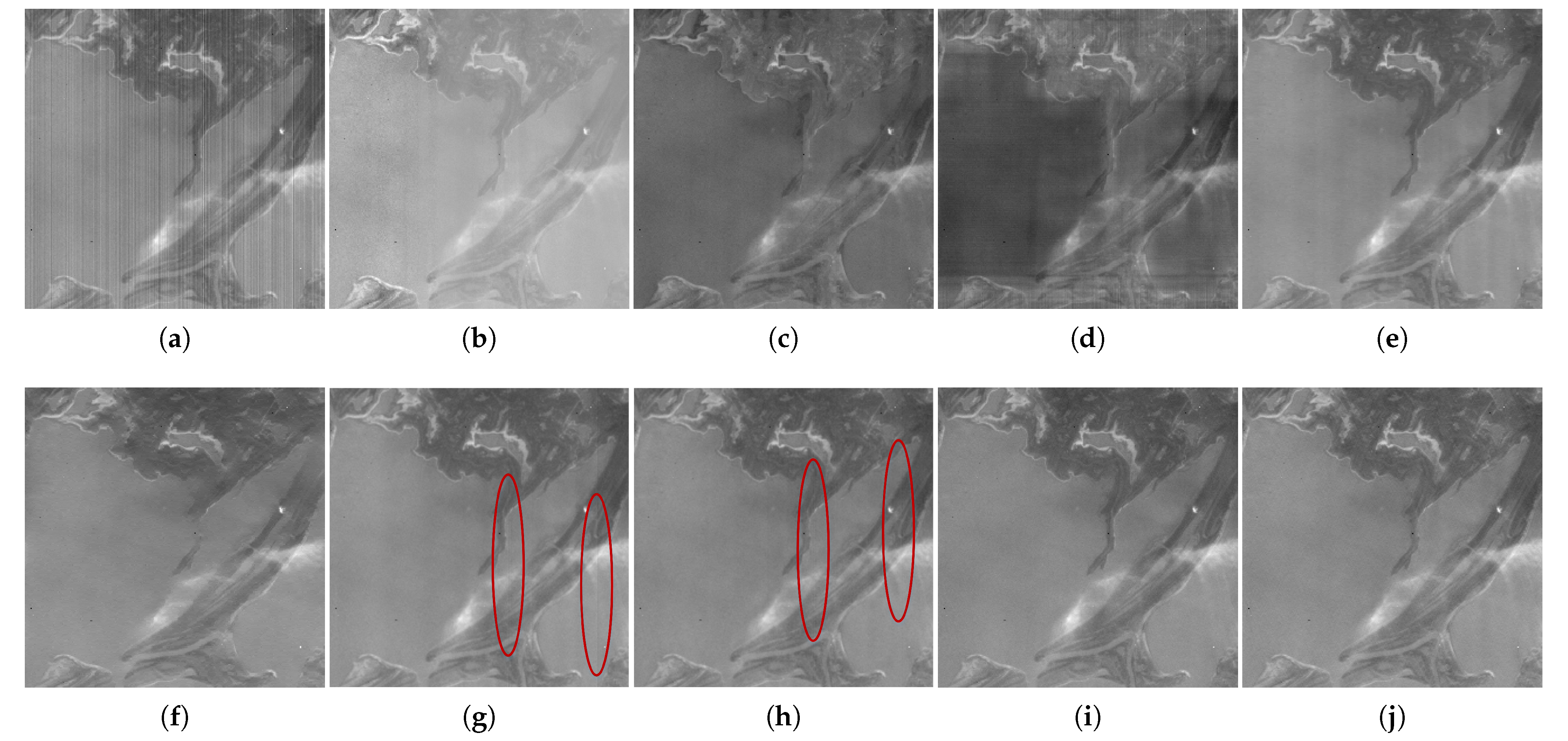
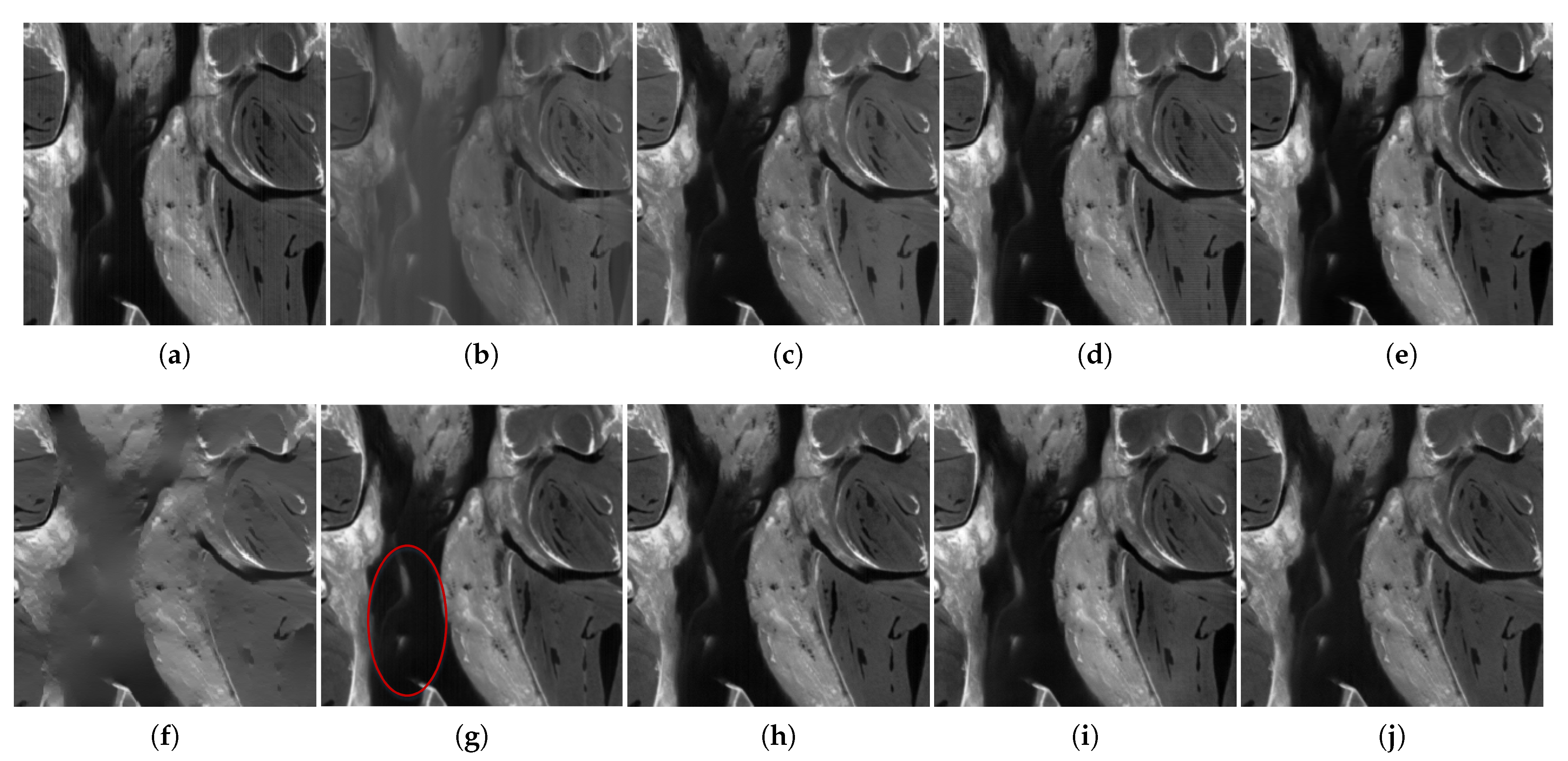
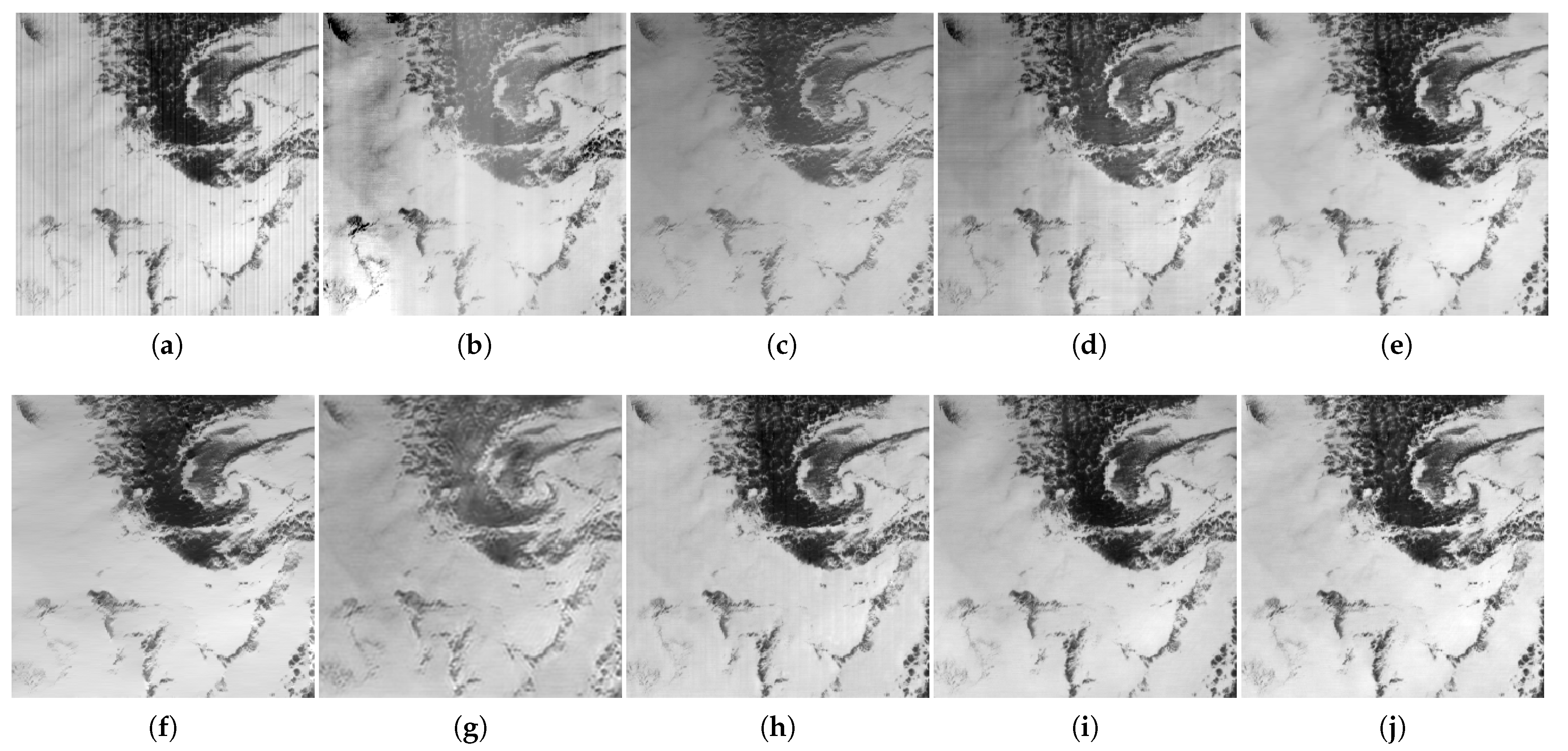
4.2. Real Image Destriping
4.2.1. Real Data
4.2.2. Evaluation
4.3. Image Uniformity
4.4. Ablation Study
4.5. Model Complexity Analysis
5. Conclusions
Author Contributions
Funding
Data Availability Statement
Conflicts of Interest
References
- Lu, X.; Wang, Y.; Yuan, Y. Graph-Regularized Low-Rank Representation for Destriping of Hyperspectral Images. IEEE Trans. Geoence Remote Sens. 2013, 51, 4009–4018. [Google Scholar] [CrossRef]
- Zhang, M.; Carder, K.; Muller-Karger, F.E.; Lee, Z.; Goldof, D.B. Noise Reduction and Atmospheric Correction for Coastal Applications of Landsat Thematic Mapper Imagery. Remote Sens. Environ. 1999, 70, 167–180. [Google Scholar] [CrossRef]
- Liu, G.; Wang, L.; Liu, D.; Fei, L.; Yang, J. Hyperspectral Image Classification Based on Non-Parallel Support Vector Machine. Remote Sens. 2022, 14, 2447. [Google Scholar] [CrossRef]
- Wang, W.; Han, Y.; Deng, C.; Li, Z. Hyperspectral Image Classification via Deep Structure Dictionary Learning. Remote Sens. 2022, 14, 2266. [Google Scholar] [CrossRef]
- Zare, A.; Gader, P. Hyperspectral Band Selection and Endmember Detection Using Sparsity Promoting Priors. IEEE Geoence Remote Sens. Lett. 2008, 5, 256–260. [Google Scholar] [CrossRef]
- Ayma Quirita, V.A.; da Costa, G.A.O.P.; Beltrán, C. A Distributed N-FINDR Cloud Computing-Based Solution for Endmembers Extraction on Large-Scale Hyperspectral Remote Sensing Data. Remote Sens. 2022, 14, 2153. [Google Scholar] [CrossRef]
- Song, M.; Li, Y.; Yang, T.; Xu, D. Spatial Potential Energy Weighted Maximum Simplex Algorithm for Hyperspectral Endmember Extraction. Remote Sens. 2022, 14, 1192. [Google Scholar] [CrossRef]
- Benhalouche, F.Z.; Benharrats, F.; Bouhlala, M.A.; Karoui, M.S. Spectral Unmixing Based Approach for Measuring Gas Flaring from VIIRS NTL Remote Sensing Data: Case of the Flare FIT-M8-101A-1U, Algeria. Remote Sens. 2022, 14, 2305. [Google Scholar] [CrossRef]
- Feng, X.; Han, L.; Dong, L. Weighted Group Sparsity-Constrained Tensor Factorization for Hyperspectral Unmixing. Remote Sens. 2022, 14, 383. [Google Scholar] [CrossRef]
- Decker, K.T.; Borghetti, B.J. Composite Style Pixel and Point Convolution-Based Deep Fusion Neural Network Architecture for the Semantic Segmentation of Hyperspectral and Lidar Data. Remote Sens. 2022, 14, 2113. [Google Scholar] [CrossRef]
- Guo, T.; Luo, F.; Fang, L.; Zhang, B. Meta-Pixel-Driven Embeddable Discriminative Target and Background Dictionary Pair Learning for Hyperspectral Target Detection. Remote Sens. 2022, 14, 481. [Google Scholar] [CrossRef]
- Hu, X.; Xie, C.; Fan, Z.; Duan, Q.; Zhang, D.; Jiang, L.; Wei, X.; Hong, D.; Li, G.; Zeng, X.; et al. Hyperspectral Anomaly Detection Using Deep Learning: A Review. Remote Sens. 2022, 14, 1973. [Google Scholar] [CrossRef]
- Wegener, M. Destriping multiple sensor imagery by improved histogram matching. Int. J. Remote Sens. 1990, 11, 859–875. [Google Scholar] [CrossRef]
- Horn, B.K.P.; Woodham, R.J. Destriping LANDSAT MSS images by histogram modification. Comput. Graph. Image Process. 1979, 10, 69–83. [Google Scholar] [CrossRef] [Green Version]
- Gadallah, F.L.; Csillag, F.; Smith, E.J.M. Destriping multisensor imagery with moment matching. Int. J. Remote Sens. 2000, 21, 2505–2511. [Google Scholar] [CrossRef]
- Liu, Z.J.; Wang, C.Y.; Wang, C. Destriping Imaging Spectrometer Data by an Improved Moment Matching Method. J. Remote Sens. 2002, 6, 279–284. [Google Scholar] [CrossRef]
- Carfantan, H.; Idier, J. Statistical Linear Destriping of Satellite-Based Pushbroom-Type Images. IEEE Trans. Geosci. Remote Sens. 2010, 48, 1860–1871. [Google Scholar] [CrossRef]
- Bouali, M.; Ladjal, S. Toward Optimal Destriping of MODIS Data Using a Unidirectional Variational Model. IEEE Trans. Geosci. Remote Sens. 2011, 49, 2924–2935. [Google Scholar] [CrossRef]
- Chang, Y.; Yan, L.; Fang, H.; Luo, C. Anisotropic Spectral-Spatial Total Variation Model for Multispectral Remote Sensing Image Destriping. IEEE Trans. Image Process. 2015, 24, 1852–1866. [Google Scholar] [CrossRef]
- Liu, X.; Lu, X.; Shen, H.; Yuan, Q.; Jiao, Y.; Zhang, L. Stripe Noise Separation and Removal in Remote Sensing Images by Consideration of the Global Sparsity and Local Variational Properties. IEEE Trans. Geosci. Remote Sens. 2016, 54, 3049–3060. [Google Scholar] [CrossRef]
- Zhang, H.; He, W.; Zhang, L.; Shen, H.; Yuan, Q. Hyperspectral Image Restoration Using Low-Rank Matrix Recovery. IEEE Trans. Geosci. Remote Sens. 2014, 52, 4729–4743. [Google Scholar] [CrossRef]
- Wang, M.; Yu, J.; Xue, J.H.; Sun, W. Denoising of Hyperspectral Images Using Group Low-Rank Representation. IEEE J. Sel. Top. Appl. Earth Obs. Remote Sens. 2016, 9, 4420–4427. [Google Scholar] [CrossRef] [Green Version]
- Chang, Y.; Yan, L.; Fang, H.; Liu, H. Simultaneous Destriping and Denoising for Remote Sensing Images With Unidirectional Total Variation and Sparse Representation. IEEE Geosci. Remote Sens. Lett. 2014, 11, 1051–1055. [Google Scholar] [CrossRef]
- Zhao, Y.Q.; Yang, J. Hyperspectral Image Denoising via Sparse Representation and Low-Rank Constraint. IEEE Trans. Geosci. Remote Sens. 2015, 53, 296–308. [Google Scholar] [CrossRef]
- Chang, Y.; Yan, L.; Wu, T.; Zhong, S. Remote Sensing Image Stripe Noise Removal: From Image Decomposition Perspective. IEEE Trans. Geosci. Remote Sens. 2016, 54, 7018–7031. [Google Scholar] [CrossRef]
- Sun, H.; Zheng, K.; Liu, M.; Li, C.; Yang, D.; Li, J. Hyperspectral Image Mixed Noise Removal Using a Subspace Projection Attention and Residual Channel Attention Network. Remote Sens. 2022, 14, 2071. [Google Scholar] [CrossRef]
- Zhang, J.; Cai, Z.; Chen, F.; Zeng, D. Hyperspectral Image Denoising via Adversarial Learning. Remote Sens. 2022, 14, 1790. [Google Scholar] [CrossRef]
- Zhang, Q.; Yuan, Q.; Li, J.; Liu, X.; Shen, H.; Zhang, L. Hybrid Noise Removal in Hyperspectral Imagery With a Spatial–Spectral Gradient Network. IEEE Trans. Geosci. Remote Sens. 2019, 57, 7317–7329. [Google Scholar] [CrossRef]
- Xiao, P.; Guo, Y.; Zhuang, P. Removing Stripe Noise From Infrared Cloud Images via Deep Convolutional Networks. IEEE Photon. J. 2018, 10, 7801114. [Google Scholar] [CrossRef]
- Kuang, X.; Sui, X.; Chen, Q.; Gu, G. Single Infrared Image Stripe Noise Removal Using Deep Convolutional Networks. IEEE Photon. J. 2017, 9, 7800615. [Google Scholar] [CrossRef]
- Crippen, R.E. A simple spatial filtering routine for the cosmetic removal of scan-line noise from Landsat TM P-tape imagery. Photogramm. Eng. Remote Sens. 1989, 55, 327–331. [Google Scholar]
- Jia, J.; Wang, Y.; Cheng, X.; Yuan, L.; Zhao, D.; Ye, Q.; Zhuang, X.; Shu, R.; Wang, J. Destriping Algorithms Based on Statistics and Spatial Filtering for Visible-to-Thermal Infrared Pushbroom Hyperspectral Imagery. IEEE Trans. Geoence Remote Sens. 2019, 57, 4077–4091. [Google Scholar] [CrossRef]
- Pande-Chhetri, R.; Abd-Elrahman, A. De-striping hyperspectral imagery using wavelet transform and adaptive frequency domain filtering. Isprs J. Photogramm. Remote Sens. 2011, 66, 620–636. [Google Scholar] [CrossRef]
- Acito, N.; Diani, M.; Corsini, G. Subspace-Based Striping Noise Reduction in Hyperspectral Images. IEEE Trans. Geoence Remote Sens. 2011, 49, 1325–1342. [Google Scholar] [CrossRef]
- Infante; Omar, S. Wavelet analysis for the elimination of striping noise in satellite images. Opt. Eng. 2001, 40, 1309–1314. [Google Scholar] [CrossRef]
- Shen, H.; Zhang, L. A MAP-Based Algorithm for Destriping and Inpainting of Remotely Sensed Images. IEEE Trans. Geosci. Remote Sens. 2009, 47, 1492–1502. [Google Scholar] [CrossRef]
- Xie, Q.; Zhao, Q.; Meng, D.; Xu, Z.; Gu, S.; Zuo, W.; Zhang, L. Multispectral Images Denoising by Intrinsic Tensor Sparsity Regularization. In Proceedings of the 2016 IEEE Conference on Computer Vision and Pattern Recognition (CVPR), Las Vegas, NV, USA, 27–30 June 2016; pp. 1692–1700. [Google Scholar] [CrossRef]
- Chang, Y.; Yan, L.; Zhong, S. Hyper-Laplacian Regularized Unidirectional Low-Rank Tensor Recovery for Multispectral Image Denoising. In Proceedings of the 2017 IEEE Conference on Computer Vision and Pattern Recognition (CVPR), Honolulu, HI, USA, 21–26 July 2017; pp. 5901–5909. [Google Scholar] [CrossRef]
- Chang, Y.; Chen, M.; Yan, L.; Zhao, X.L.; Zhong, S. Toward Universal Stripe Removal via Wavelet-Based Deep Convolutional Neural Network. IEEE Trans. Geosci. Remote Sens. 2020, 58, 2880–2897. [Google Scholar] [CrossRef]
- Chang, Y.; Yan, L.; Liu, L.; Fang, H.; Zhong, S. Infrared Aerothermal Nonuniform Correction via Deep Multiscale Residual Network. IEEE Geosci. Remote Sens. Lett. 2019, 16, 1120–1124. [Google Scholar] [CrossRef]
- Charbonnier, P.; Blanc-Feraud, L.; Aubert, G.; Barlaud, M. Two deterministic half-quadratic regularization algorithms for computed imaging. In Proceedings of the IEEE 1st International Conference on Image Processing, Austin, TX, USA, 13–16 November 1994; Volume 2, pp. 168–172. [Google Scholar] [CrossRef]
- Zhang, R. Making convolutional networks shift-invariant again. In Proceedings of the International Conference on Machine Learning (PMLR), Long Beach, CA, USA, 9–15 June 2019; pp. 7324–7334. [Google Scholar]
- Chen, Y.; Huang, T.Z.; Zhao, X.L.; Deng, L.J.; Huang, J. Stripe noise removal of remote sensing images by total variation regularization and group sparsity constraint. Remote Sens. 2017, 9, 559. [Google Scholar] [CrossRef] [Green Version]
- Dou, H.X.; Huang, T.Z.; Deng, L.J.; Zhao, X.L.; Huang, J. Directional ℓ0 Sparse Modeling for Image Stripe Noise Removal. Remote Sens. 2018, 10, 361. [Google Scholar] [CrossRef] [Green Version]
- Wang, Y.; Wei, L.; Yuan, L.; Li, C.; Lv, G.; Xie, F.; Han, G.; Shu, R.; Wang, J. New generation VNIR/SWIR/TIR airborne imaging spectrometer. In Proceedings of the International Symposium on Optoelectronic Technology and Application, Beijing, China, 9–11 May 2016. [Google Scholar] [CrossRef]
- Jia, J.; Wang, Y.; Zhuang, X.; Yao, Y.; Wang, S.; Zhao, D.; Shu, R.; Wang, J. High spatial resolution shortwave infrared imaging technology based on time delay and digital accumulation method. Infrared Phys. Technol. 2017, 81, 305–312. [Google Scholar] [CrossRef]


| Image | Index | MM | ASSTV | LRSID | Ref. [43] | PADMM | ICSRN | SSGN | CSCNet |
|---|---|---|---|---|---|---|---|---|---|
| DC | PSNR | 26.31 | 17.75 | 23.32 | 23.82 | 23.81 | 23.59 | 24.23 | 28.98 |
| SSIM | 0.89 | 0.90 | 0.90 | 0.81 | 0.81 | 0.77 | 0.82 | 0.90 | |
| Urban | PSNR | 32.86 | 23.71 | 32.87 | 29.40 | 29.49 | 29.21 | 28.05 | 34.43 |
| SSIM | 0.96 | 0.97 | 0.94 | 0.95 | 0.96 | 0.94 | 0.94 | 0.96 | |
| PaviaU | PSNR | 28.48 | 29.40 | 35.55 | 28.94 | 29.14 | 28.92 | 31.34 | 36.56 |
| SSIM | 0.95 | 0.98 | 0.98 | 0.97 | 0.98 | 0.96 | 0.98 | 0.99 | |
| Salinas | PSNR | 22.06 | 27.43 | 26.85 | 30.73 | 30.71 | 31.24 | 34.55 | 35.54 |
| SSIM | 0.82 | 0.97 | 0.94 | 0.96 | 0.95 | 0.97 | 0.98 | 0.98 |
| Intensity | Index | MM | ASSTV | LRSID | Ref. [43] | PADMM | ICSRN | SSGN | CSCNet |
|---|---|---|---|---|---|---|---|---|---|
| (−50, 50) | PSNR | 27.86 | 39.53 | 46.29 | 44.68 | 47.48 | 45.92 | 39.14 | 51.63 |
| SSIM | 0.9391 | 0.9883 | 0.9940 | 0.9916 | 0.9977 | 0.9963 | 0.9809 | 0.9989 | |
| (−100, −50) (50, 100) | PSNR | 27.80 | 37.48 | 41.94 | 39.57 | 39.97 | 43.16 | 38.97 | 50.12 |
| SSIM | 0.9365 | 0.9844 | 0.9922 | 0.9859 | 0.9925 | 0.9935 | 0.9816 | 0.9987 | |
| (−200, −100) (100, 200) | PSNR | 27.23 | 34.38 | 37.04 | 34.48 | 34.35 | 39.45 | 36.54 | 46.29 |
| SSIM | 0.9243 | 0.9749 | 0.9835 | 0.9731 | 0.9806 | 0.9898 | 0.98 | 0.9973 | |
| (−300, −200) (200, 300) | PSNR | 26.12 | 32.18 | 33.03 | 30.71 | 30.54 | 40.04 | 36.62 | 46.56 |
| SSIM | 0.9074 | 0.9628 | 0.9708 | 0.9568 | 0.9656 | 0.9900 | 0.9747 | 0.9972 |
| Item | VNIR | SWIR |
|---|---|---|
| Spectral range (m) | 0.4–0.95 | 0.95–2.5 |
| FOV (∘) | 14.7 | 14.7 |
| Detector/array size | CCD/1024 × 256 | MCT/512 × 512 |
| Spectral resolution (nm) | 2.34 | 3 |
| Band numbers | 64 | 512 |
| Method | VNIR | SWIR | CHRIS_AM | CHRIS_UK | Terra MODIS |
|---|---|---|---|---|---|
| MM | 0.0781 | 0.1042 | 0.0155 | 0.1145 | 0.1179 |
| ASSTV | 0.0445 | 0.0981 | 0.0404 | 0.0528 | 0.0436 |
| LRSID | 0.0464 | 0.0793 | 0.0567 | 0.0172 | 0.0418 |
| Ref. [43] | 0.0182 | 0.1153 | 0.0396 | 0.0533 | 0.0093 |
| PADMM | 0.1526 | 0.1758 | 0.0622 | 0.6424 | 0.0201 |
| ICSRN | 0.0100 | 0.0586 | 0.0070 | 0.0131 | 0.0754 |
| SSGN | 0.0235 | 0.0614 | 0.0085 | 0.0177 | 0.0077 |
| TSWEU | 0.1049 | 0.2142 | 0.0630 | 0.1432 | 0.0758 |
| CSCNet | 0.0112 | 0.0713 | 0.0082 | 0.0163 | 0.0196 |
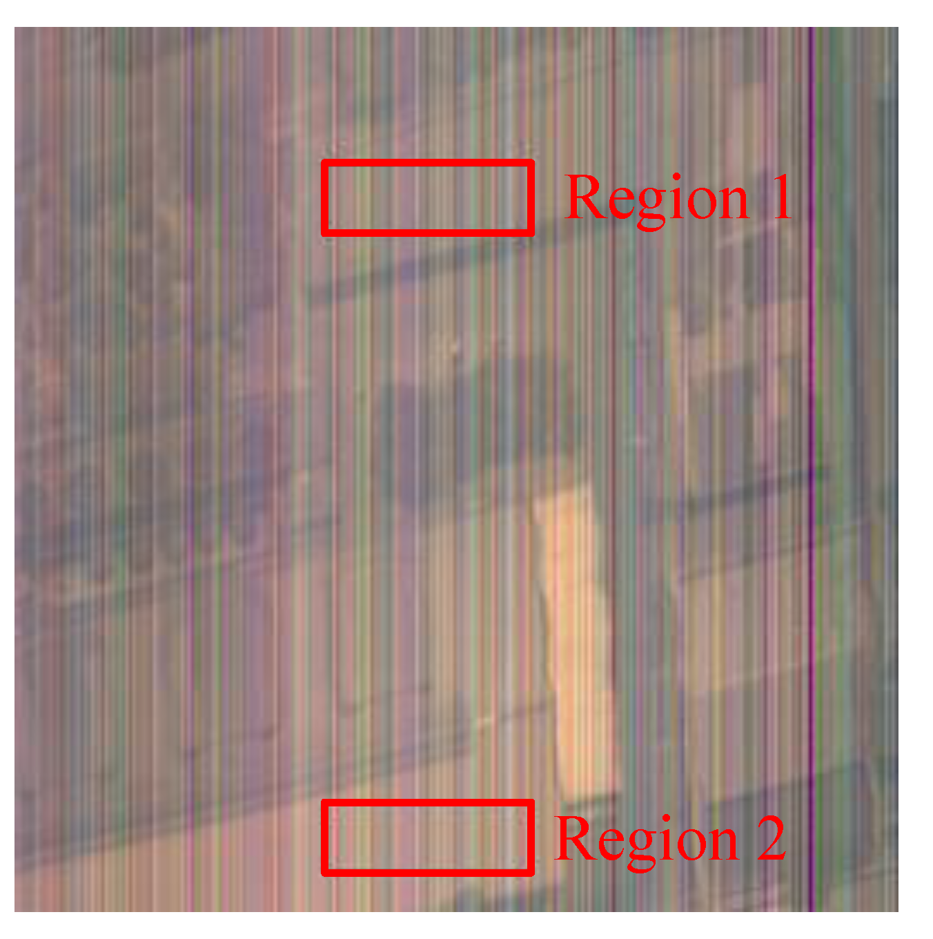
| Method | MM | ASSTV | LRSID | Ref. [43] | PADMM | ICSRN | SSGN | TSWEU | CSCNet |
|---|---|---|---|---|---|---|---|---|---|
| Region1 | 0.0556 | 0.0561 | 0.0556 | 0.0787 | 0.0611 | 0.0535 | 0.0514 | 0.0919 | 0.0548 |
| Region2 | 0.0411 | 0.0232 | 0.0219 | 0.0271 | 0.0350 | 0.0221 | 0.0211 | 0.0181 | 0.0206 |
| Method | ICSRN | SSGN | TSWEU | Lite-CSCNet | CSCNet |
| Parameters (M) | 0.8 | 0.2 | 3.2 | 3.1 | 6.2 |
| Flops (G) | 54 | 11 | 103 | 90 | 175 |
| Method | MM | ASSTV | LRSID | Ref. [43] | PADMM | ICSRN | SSGN | TSWEU | Lite-CSCNet | CSCNet |
| Time | 0.01 | 9.93 | 44.47 | 6.31 | 3.99 | 0.26 | 0.07 | 0.45 | 0.35 | 0.61 |
Publisher’s Note: MDPI stays neutral with regard to jurisdictional claims in published maps and institutional affiliations. |
© 2022 by the authors. Licensee MDPI, Basel, Switzerland. This article is an open access article distributed under the terms and conditions of the Creative Commons Attribution (CC BY) license (https://creativecommons.org/licenses/by/4.0/).
Share and Cite
Li, J.; Zeng, D.; Zhang, J.; Han, J.; Mei, T. Column-Spatial Correction Network for Remote Sensing Image Destriping. Remote Sens. 2022, 14, 3376. https://doi.org/10.3390/rs14143376
Li J, Zeng D, Zhang J, Han J, Mei T. Column-Spatial Correction Network for Remote Sensing Image Destriping. Remote Sensing. 2022; 14(14):3376. https://doi.org/10.3390/rs14143376
Chicago/Turabian StyleLi, Jia, Dan Zeng, Junjie Zhang, Jungong Han, and Tao Mei. 2022. "Column-Spatial Correction Network for Remote Sensing Image Destriping" Remote Sensing 14, no. 14: 3376. https://doi.org/10.3390/rs14143376
APA StyleLi, J., Zeng, D., Zhang, J., Han, J., & Mei, T. (2022). Column-Spatial Correction Network for Remote Sensing Image Destriping. Remote Sensing, 14(14), 3376. https://doi.org/10.3390/rs14143376