Near-Field Multiple Target Localization in Frequency Diverse Array Based on Tensor Decomposition

Abstract

Target localization is a fundamental problem in array signal processing. The problem of locating near-field targets with multiple-input multiple-output (MIMO) radar has been studied extensively; however, most of the conventional matrix-based approaches suffer from limitations in terms of the representation and exploitation of the multidimensional nature of MIMO radar signals. In this paper, we addressed the problem of localizing multiple targets in the near-field region, aiming at pursuing a solution applicable for multidimensional signal that is able to achieve sufficient accuracy. A tensor-based signal model impinging on a monostatic frequency diverse array multiple-input multiple-output (FDA-MIMO) radar was formulated, and a corresponding tensor decomposition-based localization algorithm (TenDLA) that showcases the connection between the tensor-based analysis and the localization problem was developed. Additionally, a correction procedure to mitigate the estimation deviations on the range and angle was presented, yielding significant improvements in estimation accuracy. Numerical examples demonstrated the validity and effectiveness of the proposed approach, and it was shown that this approach is superior to conventional methods due to its high-resolution estimation accuracy as well as its relatively low computational costs.

1. Introduction

Near-field target localization has attracted considerable attention in recent research, as this technique is widely applied from daily applications to scientific research, such as automotive driving, indoor positioning, speech enhancement, and underground investigations [1,2,3,4,5]. Similar to far-field target localization, near-field target localization is aimed at finding the direction and distance of identifiable targets. However, it is certain that the thoroughly studied far-field target localization techniques are not applicable in near-field situations, as the wavefront is considered as a plane wave under far-field assumptions, while waves propagated in the near-field scenario have a spherical wavefront; hence, the phase difference across the array is characterized by a nonlinear function of both the azimuth angle and range [6]. This characteristic makes the parameter estimation issue more challenging for near-field targets than it is for the existing far-field approaches.

There have been numerous related works focused on near-field target localization or source localization, which can be found in refs. [6,7,8,9,10,11,12,13]. These works realized distinct approaches and algorithms, including classic spectral searching methods (e.g., two-dimensional MUSIC (2D-MUSIC) [6] and Capon [7]), subarray-based method (e.g., ESPRIT [8]), the maximum-likelihood estimator (MLE) [9], second-order statistics (SOS) based methods [10,11], and higher-order statistics (HOS) based methods [12,13]. Nevertheless, most of these methods suffer from limitations, such as the heavy computational burden owing to multidimensional searching (e.g., MUSIC or MLE), massive efforts on eigen-decomposition (e.g., subspace-based or HOS), and the restriction on array geometry (e.g., subarray-based). Thus, this motivates us to seek a novel approach that provides sufficiently good performance that is only at the cost of relatively low computation consumption.

On the other hand, the implementation of radar systems is another matter to be concerned about. Although most of the aforementioned methods are implemented via MIMO radar, due to its advantages of flexible waveform diversity and spatial diversity [14], the coupling of angle and range in the near-field signal model means that the estimation of the location parameters cannot be resolved directly. Different from conventional MIMO radar, the combination of FDA and MIMO radar that is referred to as the FDA-MIMO radar, which can provide a range-angle-dependent beampattern and maintain the superiorities of MIMO radar [15,16,17], paves a new way to resolve the parameter estimation problem. Several related studies have been conducted during the past decade [18,19,20,21], with almost all of these approaches being applicable to the far-field model. To our knowledge, the application of FDA-MIMO for near-field targets has been seldom reported in the literature. Furthermore, FDA-MIMO radar signals are essentially multidimensional, and the matrix-based representation and analysis in conventional methods cannot fully exploit the inherent algebraic structure of these multidimensional data [22,23], this problem requires further investigation.

Tensor algebra and tensor analysis allow us to deal with high-dimensional signals from a new perspective [24,25,26]. Literature addressing the problem of target localization based on tensor analysis can be found in refs. [27,28,29,30,31,32] for far-field targets and in refs. [33,34,35,36,37] for near-field targets. The authors of [27] systematically developed tensor-based signal model formulations and their corresponding solutions under three types of MIMO radar configurations, establishing a theoretical foundation for follow-up studies, including trilinear-decomposition based methods [29,30]; the unitary parallel factor (PARAFAC) method [31]; and the higher-order singular value decomposition (HOSVD) method [32]. However, directly extending these methods to near-field situations degrades their performance, and the methods may even fail, owing to the nonlinear property in the signal model. In contrast, ref. [33] used a quadric wavefront approximation model for the two-dimensional near-field localization problem and successfully achieved target parameter estimation based on tensor decomposition. However, there was a non-neglected systematic error in the estimated range and angle caused by the use of the Fresnel approximation model [34], leading to a degradation in accuracy. To overcome this drawback, some effective approaches have been proposed via the correction procedure [35] or via formulation with an exact model [36,37]. The above tensor-based approaches exhibit significant superiority over conventional methods, which motivates us to establish a solution based on the power of multilinear algebra rather than on conventional matrix-based methods.

In this paper, we focus on the problem of localizing multiple targets in the near-field region via a symmetric monostatic FDA-MIMO radar. Motivated by the existing tensor-based signal model that is applicable to far-field scenarios, we extend it to near-field situations and propose a corresponding parameter estimation approach by leveraging the power of tensor analysis and the advantage of FDA-MIMO radar. The main contributions of this paper are summarized as follows:

1) A tensor-based signal model applicable to near-field multiple target localization is formulated in this work. Meanwhile, an improved trilinear decomposition algorithm is introduced to improve the numerical stability when solving tensor decomposition.

2) A novel target localization algorithm named TenDLA is developed based on tensor analysis. Joint range and angle estimation can be solved using TenDLA with relatively good accuracy, and the aforementioned systematic errors encountered in some existing localization methods are mitigated effectively.

3) Compared to conventional methods, the proposed tensor-based method has the merits of simplicity and efficiency, owing to its advantage of search-free and automatic pairing.

The remainder of this paper is organized as follows. Section 2 introduces the signal model of monostatic FDA-MIMO radar. In Section 3, the proposed joint estimation of angle and range as well as the corresponding correction procedure are presented. The performance analysis and numerical simulations are presented in Section 4 and Section 5, respectively. Finally, conclusions are drawn in Section 6.

Notations: (.)^*, (.)^T, (.)⁻¹ and (.)^† denote the complex conjugation, transpose, inverse and psedo-inverse operations, respectively. $\left|\right|{.\left|\right|}_F$ stands for the Frobenius norm and diag(a) stands for the diagonal matrix of vector a. Scalars, column vectors, matrices, and tensors are denoted by lowercase letters, boldface lowercase letters, boldface uppercase letters and calligraphic uppercase letters, respectively, such as $x,\mathit{x},X\mathrm{and}\mathcal{X}$. The symbol of $\otimes$, $\odot$, $\oplus$ and $\circ$ represent the Kronecker product, Khatri-Rao product, Hadamard product and the vector outer product, respectively. Definitions of product rules used in this paper are given in

Table 1. Definitions of product rules.

Notation	Definition
$C=A\otimes B$	The Kronecker product of matrices $A\in {ℂ}^{I\times J}$ and ${\rm B}\in {ℂ}^{K\times L}$ yields $C=\left[a_1\otimes b_1,a_1\otimes b_2,\cdots ,a_J\otimes b_{L-1},a_J\otimes b_L\right]\in {ℂ}^{(I\times K)\times (J\times L)}$.
$C=A\odot B$	The Khatri-Rao product of matrices $A\in {ℂ}^{I\times K}$ and ${\rm B}\in {ℂ}^{J\times K}$ yields $C\in {ℂ}^{(I\times J)\times K}$ with columns $c_k=a_k\otimes b_k$.
$C=A\oplus B$	The Hadamard product of matrices $A\in {ℂ}^{I\times J}$ and ${\rm B}\in {ℂ}^{I\times J}$ yields $C\in {ℂ}^{I\times J}$ with entries $c_{ij}=a_{ij}{b}_{ij}$.
$\mathcal{X}=a^{(1)}\circ a^{(2)}\circ \cdots \circ a^{(N)}$	The outer product of vectors $a^{(n)}\in {ℂ}^{I_n}$ yields a rank-one tensor $\mathcal{X}\in {ℂ}^{I_1\times I_2\times \cdots \times I_N}$$\mathrm{with}\mathrm{entries}{x}_{I_1}{{}_{I_2}}_{\cdots I_N}=a_{I_1}^{(1)}{a}_{I_2}^{(2)}\cdots a_{I_N}^{(N)}$.

.

2. Signal Model

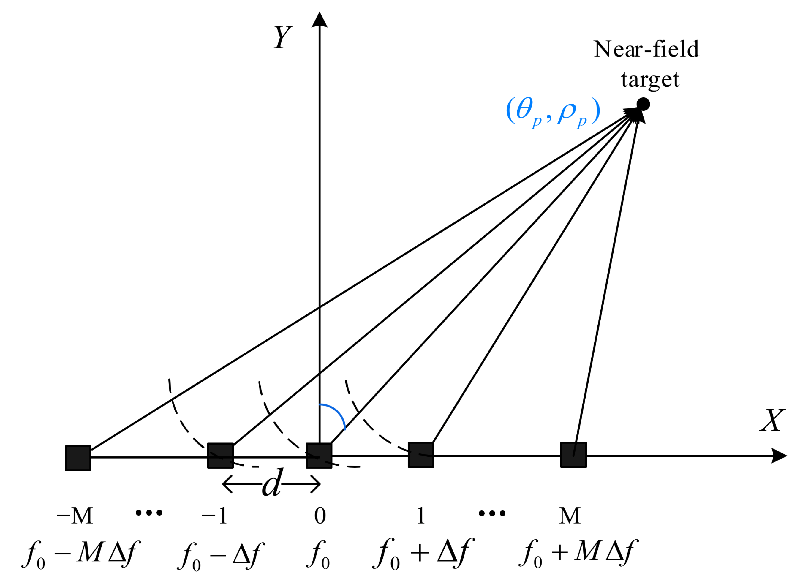
We consider a symmetric monostatic FDA-MIMO radar system in which the transmitter is an FDA and the receiver is a phased array. As shown in Figure 1, the FDA-MIMO radar consists of 2M + 1 uniformly spaced transceiver antennas, and the transmit array and receive array are collocated. There are P uncorrelated targets located away from the antenna array with deterministic location parameters {θ_p, ρ_p}, where θ_p and ρ_p are the angle and range of the pth target relative to the center of the antenna array, respectively. It is assumed that all of the targets in this paper are located in the near-field region (also called the Fresnel region [38]) of the antenna array, i.e., the distance between the target and antenna array is within the range of [0.62(D³/λ)^1/2, 2D²/λ], where D is the array’s aperture given by D = 2Md, and d is the array element spacing.

We assume that the carrier frequency and the transmitted signal of the mth transmit antenna are given as

$$f_m=f_0+m\Delta f,m=-M,\dots ,0,\dots ,M$$

(1)

and

$$s_m(t)=\mathrm{rect}\left(\frac{t}{T_p}\right){\varphi }_m(t)e^{j2\pi f_{m}t},0\le t\le T_p$$

(2)

where f₀ is the carrier frequency of the reference element in the transmit array, Δf is the linear frequency increment between adjacent elements, ${\varphi }_m$ denotes the mth orthogonal baseband waveform with unit power, and T_p is the radar pulse duration. Without loss of generality, we assume that the entire radar detection process consists of L consecutive pulses.

Let the array center be the phase reference point, then the signal received by the nth element can be expressed as

$$x_n(t)={\displaystyle \sum _{p=1}^P{\displaystyle \sum _{m=-M}^M\mathrm{rect}\left\{\frac{t-{\tau }_{\mathrm{t},(m,p)}-{\tau }_{\mathrm{r},(n,p)}}{T_p}\right\}{\beta }_p(t)}}{\varphi }_m(t-{\tau }_{\mathrm{t},(m,p)}-{\tau }_{\mathrm{r},(n,p)})e^{j2\pi f_m\left(t-{\tau }_{\mathrm{t},(m,p)}-{\tau }_{\mathrm{r},(n,p)}\right)}$$

(3)

where β_p(t) is the complex-valued reflection coefficient of the pth target, and t denotes the sampling instant. τ_t,(m,p) and τ_r,(n,p) are the transmit and receive time delays, respectively, which have a positive correlation with the wave path differences of ${\delta }_{\mathrm{t},(m,p)}$ and ${\delta }_{\mathrm{r},(n,p)}$, which are given as.

$${\delta }_{\mathrm{t},(m,p)}=\sqrt{{({\rho }_p\sin {\theta }_p-md)}^2+{({\rho }_p\cos {\theta }_p)}^2}-{\rho }_p$$

(4)

and

$${\delta }_{\mathrm{r},(n,p)}=\sqrt{{({\rho }_p\sin {\theta }_p-nd)}^2+{({\rho }_p\cos {\theta }_p)}^2}-{\rho }_p$$

(5)

Since the path difference in the signal model is a nonlinear function of range and angle, one general decoupling strategy with lower computational complexity is to approximate the path difference with second-order Taylor expansion, e.g., refs. [8,10]. It follows that the approximation of (4) and (5) are denoted as

$${\tilde{\delta }}_{\mathrm{t},(m,p)}=m{\omega }_p+m^2{\phi }_p$$

(6)

and

$${\tilde{\delta }}_{\mathrm{r},(m,p)}=n{\omega }_p+n^2{\phi }_p$$

(7)

where ω_p = −dsin(θ_p), φ_p = [d²cos²(θ_p)/ρ_p]/2.

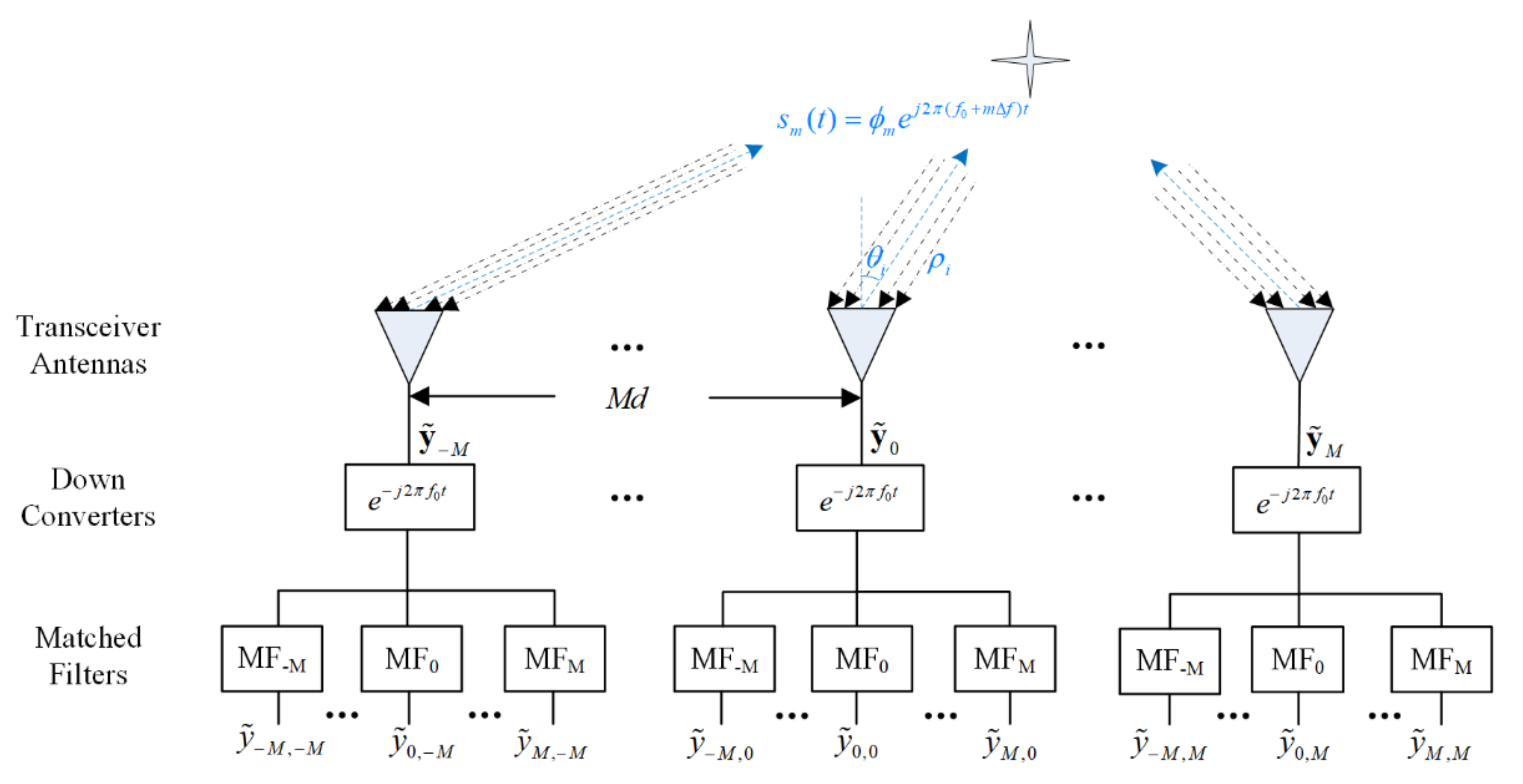
After coherent processing and matched filtering as shown in Figure 2, the output of the receiver array for the lth pulse period can be stacked as a column vector, which is written as

$$x_{\mathrm{s}}(l)={\displaystyle \sum _{p=1}^P{\beta }_p(l)a_{\mathrm{r}}({\theta }_p,{\rho }_p)\otimes a_{\mathrm{t}}({\theta }_p,{\rho }_p)}$$

(8)

where $a_{\mathrm{r}}({\theta }_p,{\rho }_p)$ and $a_{\mathrm{t}}({\theta }_p,{\rho }_p)$ denote the receive and transmit steering vector with respect to the pth target, respectively, which are given by.

$$a_{\mathrm{r}}({\theta }_p,{\rho }_p)=\left[\begin{array}{c}{e}^{j\frac{2\pi }{\lambda }\left\{(-M)d\sin {\theta }_p-\frac{1}{2}\frac{{(-M)}^2{(d\cos {\theta }_p)}^2}{{\rho }_p}\right\}}\\ ⋮\\ e^{j\frac{2\pi }{\lambda }\left\{(M)d\sin {\theta }_p-\frac{1}{2}\frac{M^2{(d\cos {\theta }_p)}^2}{{\rho }_p}\right\}}\end{array}\right]$$

(9)

and

$$a_{\mathrm{t}}({\theta }_p,{\rho }_p)=\left[\begin{array}{c}{e}^{j\frac{2\pi }{\lambda }\left\{(-M)d\sin {\theta }_p-\frac{1}{2}\frac{{(-M)}^2{(d\cos {\theta }_p)}^2}{{\rho }_p}-(-M)\frac{2{\rho }_p\Delta f}{f_0}\right\}}\\ ⋮\\ e^{j\frac{2\pi }{\lambda }\left\{Md\sin {\theta }_p-\frac{1}{2}\frac{M^2{(d\cos {\theta }_p)}^2}{{\rho }_p}-M\frac{2{\rho }_p\Delta f}{f_0}\right\}}\end{array}\right]$$

(10)

Now let us consider the coherent processing interval (CPI) with L consecutive pulses. For some specific applications, such as low-slow-small (LSS) target detection, the radar cross section coefficient (RCS) of the target is no longer constant during the CPI, i.e., the RCS of the target fluctuates from time to time. Under this circumstance, the general scheme to fit the RCS fluctuations is modeled using the Swerling II target model [39]. It follows that the final output of the radar system with L consecutive pulses can be written as the following compact form, which is based on the derivations in refs. [18,27].

$$X_{\mathrm{s}}=\left[x_{\mathrm{s}}(1),x_{\mathrm{s}}(2),\cdots ,x_{\mathrm{s}}(L)\right]+N=A_{\mathrm{r}}(\theta ,\rho )\odot A_{\mathrm{t}}(\theta ,\rho )S^T+N$$

(11)

Herein, we take into consideration the impact of noise in realistic scenarios, where N is the additive noise term and is typically modeled as additive white Gaussian noise (AWGN), $A_{\mathrm{r}}(\theta ,\rho )\in {ℂ}^{(2M+1)\times P}$ and $A_{\mathrm{t}}(\theta ,\rho )\in {ℂ}^{(2M+1)\times P}$ denote the receive and transmit steering matrices, respectively, and $S\in {ℂ}^{L\times P}$ is the RCS coefficient matrix containing the complete RCS information during the CPI, which is defined by $S=[s\left(1\right),\cdots ,s(L{\left)\right]}^T$ and $s\left(l)=[{\beta }_1\right(l),\cdots ,{\beta }_P(l\left)\right]$.

Based on multilinear algebra, (11) is a typical three-way parallel factor (PARAFAC) model, i.e., Xs is the matrix unfolding of a three-order tensor $\mathcal{X}\in {ℂ}^{(2M+1)\times (2M+1)\times L}$, whereas $\mathcal{X}\in {ℂ}^{(2M+1)\times (2M+1)\times L}$ can be tensorized from its unfolding form. As discussed in the Introduction section, conventional matrix-based approaches only exploit the pairwise interactions of this flattened model, in other words, only the “one-dimensional” information is used, which leads to performance deterioration, especially in lower signal-to-noise-ratio (SNR) cases; see [23,32]. To overcome this limitation, by leveraging the power of multilinear algebra, we reformatted the data model to be a tensor-based signal model, making it possible to exploit the multiple interactions and couplings hidden in the multidimensional nature of received signals. Detailed analysis and derivations are provided in the following sections.

3. The Proposed Approach

In this section, we present the solution to the joint range and angle estimation problem via mathematical explanation and derivation. We first explore the issue of achieving reliable estimation of the whole directional matrices. Then, the joint range and angle estimation is resolved using a two-step estimation procedure, and the corresponding correction method to mitigate systematic bias is finally proposed.

3.1. Overview of Methods

The basic flow of the proposed tensor-based near-field target localization approach is illustrated in Figure 3. Firstly, FDA radar transmits consecutive pulses to scan areas of interest, and the echoes reflected by multiple targets are then received and sampled by receive antennas. After multistage signal processing procedures have been carried out, including synchronization, matched filtering, and rearranging, the outputs obtained in the receive array are converted into a trilinear data structure. Based on this PARAFACT model, it is possible to transform the localization issue into an algebraic decomposition problem, under the commonly used CANDECOMP/PARAFAC (CP) decomposition framework. Finally, the joint range and angle estimation can be resolved from the obtained estimates of the factor matrices, via the use of certain conventional parameter estimation algorithms, e.g., LS approximation, MLE, etc. A detailed description of the algorithm will be presented at the end of Section 3.

3.2. Estimation of the Steering Matrices

In order to accurately estimate the factor matrices from the observed tensor $\tilde{\mathcal{X}}$, solving the CP decomposition of $\tilde{\mathcal{X}}$ is the primary task. The most extensively used approach is the well-known alternating least squares (ALS) algorithm proposed in ref. [24], in which the problem can be settled by minimizing the following optimization cost functions:

$$A_{\mathrm{r}}=\underset{A_r}{\arg \min }\left|\right|{\tilde{X}}_{\left(1\right)}-A_{\mathrm{r}}{(S\odot A_{\mathrm{t}})}^T|{|}_F^2$$

(12)

$$A_{\mathrm{t}}=\underset{A_t}{\arg \min }\left|\right|{\tilde{X}}_{(2)}-A_{\mathrm{t}}{(S\odot A_{\mathrm{r}})}^T|{|}_F^2$$

(13)

$$S=\underset{S}{\arg \min }\left|\right|{\tilde{X}}_{(3)}-S{(A_{\mathrm{t}}\odot A_{\mathrm{r}})}^T|{|}_F^2$$

(14)

where ${\tilde{X}}_{\left(1\right)}$, ${\tilde{X}}_{\left(2\right)}$ and ${\tilde{X}}_{\left(3\right)}$ denote the mode-n (n = 1, 2, 3) matricization of tensor $\tilde{\mathcal{X}}$ respectively.

The ALS approach of solving (12)–(14) can be achieved by implementing LS fitting for each cost function, i.e., fix A_t and S to solve for A_r, and then repeat the above procedures given below alternatively until the convergence criterion is satisfied:

$$A_{\mathrm{r}}={\tilde{X}}_{\left(1\right)}[(S\odot A_{\mathrm{t}}){(S^{T}S\oplus A_{\mathrm{t}}{}^T{A}_{\mathrm{t}})}^{†}]$$

(15)

$$A_{\mathrm{t}}={\tilde{X}}_{\left(2\right)}[(S\odot A_{\mathrm{r}}){(S^{T}S\oplus A_{\mathrm{r}}{}^T{A}_{\mathrm{r}})}^{†}]$$

(16)

$$S={\tilde{X}}_{\left(3\right)}[(A_{\mathrm{t}}\odot A_{\mathrm{r}}){(A_{\mathrm{t}}{}^T{A}_{\mathrm{t}}\oplus A_{\mathrm{r}}{}^T{A}_{\mathrm{r}})}^{†}]$$

(17)

ALS is simple and that this is the reason why it is widely applied, but the problem of slow convergence encountered in some ill-conditioned cases, which is referred to as the swamp [40], leads to degradation when solving for the factor matrices. Swamps may be caused by various reasons, e.g., the initialization of the factor matrices or collinearity in the factor matrices. To overcome this drawback, we utilized an improved algorithm called regularized ALS (RALS) instead of using ALS, which is proven to be effective in solving the CP decomposition, according to the theoretical analysis and numerical simulations in ref. [41]. Thus, by adding regularization term to the LS estimators, the expressions (15)–(17) can be rewritten as

$$A_{\mathrm{r}}{}^{(k+1)}=[{\tilde{X}}_{\left(1\right)}(S^{(k)}\odot A_{\mathrm{t}}{}^{(k)})+{\tau }^{(k)}{A}_{\mathrm{r}}{}^{(k)}]\times {[{(S^{(k)})}^T{S}^{(k)}\oplus {(A_{\mathrm{t}}{}^{(k)})}^T{A}_{\mathrm{t}}{}^{(k)}+{\tau }^{(k)}I]}^{-1}$$

(18)

$$A_{\mathrm{t}}{}^{(k+1)}=[{\tilde{X}}_{\left(2\right)}(S^{(k)}\odot A_{\mathrm{r}}{}^{(k+1)})+{\tau }^{(k)}{A}_{\mathrm{t}}{}^{(k)}]\times {[{(S^{(k)})}^T{S}^{(k)}\oplus {(A_{\mathrm{r}}{}^{(k+1)})}^T{A}_{\mathrm{r}}{}^{(k+1)}+{\tau }^{(k)}I]}^{-1}$$

(19)

$$S^{(k+1)}=[{\tilde{X}}_{\left(3\right)}(A_{\mathrm{t}}{}^{(k+1)}\odot A_{\mathrm{r}}{}^{(k+1)})+{\tau }^{(k)}{S}^{(k)}]\times {[{(A_{\mathrm{t}}{}^{(k+1)})}^T{A}_{\mathrm{t}}{}^{(k+1)}\oplus {(A_{\mathrm{r}}{}^{(k+1)})}^T{A}_{\mathrm{r}}{}^{(k+1)}+{\tau }^{(k)}I]}^{-1}$$

(20)

where τ^(k) is the regularization parameter and is updated after every iteration of the loop by the equation of τ^(k+1) = δ·τ^(k). Herein parameter δ is the scaling factor, which is a constant and is greater than zero in general. I is the identity matrix.

The operation of adding regularization terms makes the update of the factor matrix after every iteration is weakly correlated with previous results, resulting in the outcomes of every iteration being smoother than those of the ALS algorithm [42]. Furthermore, the regularized cost functions are component-wise strictly quasiconvex, and this contributes to the guarantee of convergence [41]. Therefore, the introduced RALS algorithm enhances the numerical stability of solving the CP decomposition, which is characterized as removing (if not, shortening) the swamp problem to some degree; thereby it is possible to improve the level of reliability when solving target parameters.

3.3. Joint Range and Angle Estimation for Multiple Targets

In the previous works of [29,30], the estimation of direction-of-angle (DoA) can be resolved by LS estimation directly after obtaining the estimates of ${\widehat{A}}_{\mathrm{r}}$ and ${\widehat{A}}_{\mathrm{t}}$. However, since the path difference in near-field situations is characterized by a combined function of angle and range, the existing far-field model based methods are no longer valid. Moreover, owing to the property of the FDA, the signal model is quite different from its counterpart in conventional MIMO radar, which contains an extra range-frequency-dependent term. Therefore, it is necessary to develop an improved solution for joint range and angle estimation that is applicable to the near-field model impinging on FDA-MIMO radar.

3.3.1. Data Pre-processing Procedure

One solution for dealing with the problem of decoupling the angle and range from the combined signal model is to exploit the cross-correlation across the symmetrical array [43]. Before that, a normalization operation is first required. Then, similar to [43], we can separate the first-order phase terms (i.e., angle-dependent only) from ${\widehat{A}}_{\mathrm{r}}$ by

$${\widehat{A}}_{\mathrm{r}}^{\left(\mathrm{odd}\right)}=J_M{\widehat{A}}_{\mathrm{r}}\oplus {\widehat{A}}_{\mathrm{r}}{}^{*}$$

(21)

where $J_M\in {ℂ}^{(2M+1)(2M+1)}$ is the unitary anti-diagonal matrix. Equivalently, the second-order phase terms (i.e., the angle-range-combined terms) can be extracted as follows:

$${\widehat{A}}_{\mathrm{r}}^{\left(\mathrm{even}\right)}=J_M{\widehat{A}}_{\mathrm{r}}\oplus {\widehat{A}}_{\mathrm{r}}$$

(22)

For the transmit steering matrix ${\widehat{A}}_{\mathrm{t}}$, we can perform the same transforms to obtain ${\widehat{A}}_{\mathrm{t}}^{\left(\mathrm{odd}\right)}$ and ${\widehat{A}}_{\mathrm{t}}^{\left(\mathrm{even}\right)}$ as well. It is worth noting that, the separated first-order phase term ${\widehat{A}}_{\mathrm{t}}^{\left(\mathrm{odd}\right)}$ regarding the transmit steering matrix contains a set of extra range-frequency-dependent components, which are distinct from their counterparts in the receive steering matrix. Relying on this, it is possible to solve the ρ_p if these components are extracted from the phase factor of ${\widehat{A}}_{\mathrm{t}}$. We will develop the procedure later on.

3.3.2. Unambiguous Estimation of Range

As previously mentioned, the range parameter can be resolved according to the specific array structure of ${\widehat{A}}_{\mathrm{t}}$. However, the inherent phase period ambiguity problem introduced by the FDA is the other annoyance to be resolved. This problem arises due to the phase angle of one component in (10) being ambiguous, i.e., there are several possible solutions in the range domain with an uncertain additional phase angle of 2kπ. The ambiguous phase angle Ω can be expressed as

$${\Omega }_{t,(m,p)}=2\pi \left[m\frac{d\sin \theta }{\lambda }-\frac{1}{2}\frac{m^2{(d\cos {\theta }_p)}^2}{\lambda {\rho }_p}-m\frac{2{\rho }_p\Delta f}{c_0}\right]\in [-\pi -2k\pi ,\pi -2k\pi ]$$

(23)

where m = −M, …, M, k ∊ N. Obviously, range estimation cannot be solved until the coefficient k is determined. To deal with this ambiguity problem, the proposed unambiguous solution for range is developed below.

Let us consider the array structure of ${\widehat{A}}_{\mathrm{t}}^{\left(\mathrm{odd}\right)}$. For simplicity, only consider the solution for the pth target as an example. The other targets can be resolved using the same procedures. The pth column vector of ${\widehat{A}}_{\mathrm{t}}^{\left(\mathrm{odd}\right)}$ is as seen below:

$${\widehat{a}}_{\mathrm{t},p}^{\left(\mathrm{odd}\right)}=\left[\begin{array}{c}{e}^{j2\pi \left\{-2M\frac{{\widehat{\omega }}_p}{\lambda }+\frac{2{\widehat{\rho }}_p}{c_0}\left(\Delta f_{(-M,0)}-\Delta f_{(M,0)}\right)\right\}}\\ ⋮\\ e^{j2\pi \left\{2M\frac{{\widehat{\omega }}_p}{\lambda }+\frac{2{\widehat{\rho }}_p}{c_0}\left(\Delta f_{(M,0)}-\Delta f_{(-M,0)}\right)\right\}}\end{array}\right]$$

(24)

where Δf_(m,0) indicates the frequency offset between the mth element and the reference element, denoted by Δf_(m,0) = f_m − f₀, m = −M, …,M. By means of the angle operation, the ambiguous phase angle ${\widehat{h}}_{\mathrm{t},p}$ is given as.

$${\widehat{h}}_{\mathrm{t},p}=angle({\widehat{a}}_{\mathrm{t},p}^{\left(\mathrm{odd}\right)})=2\pi \left\{\left[\begin{array}{c}-2M\frac{{\widehat{\omega }}_p}{\lambda }+\frac{2{\widehat{\rho }}_p}{c_0}(\Delta f_{-M,M})\\ ⋮\\ 2M\frac{{\widehat{\omega }}_p}{\lambda }+\frac{2{\widehat{\rho }}_p}{c_0}(\Delta f_{M,-M})\end{array}\right]-\left[\begin{array}{c}{k}_{\mathrm{t},-M}\\ ⋮\\ k_{\mathrm{t},M}\end{array}\right]\right\}$$

(25)

where k_t,m is an unknown integer. Let the first 2M equations subtract the last 2M equations, and a new linear system with respect to ${\widehat{\rho }}_p$ is obtained.

$$\frac{1}{2\pi }\left[\begin{array}{c}angle\left(\frac{{\widehat{a}}_{\mathrm{t},p}^{\left(\mathrm{odd}\right)}(-M)}{{\widehat{a}}_{\mathrm{t},p}^{\left(\mathrm{odd}\right)}(-M+1)}\right)\\ ⋮\\ angle\left(\frac{{\widehat{a}}_{\mathrm{t},p}^{\left(\mathrm{odd}\right)}(M-1)}{{\widehat{a}}_{\mathrm{t},p}^{\left(\mathrm{odd}\right)}(M)}\right)\end{array}\right]=-\frac{2{\widehat{\omega }}_p}{\lambda }+\frac{2{\widehat{\rho }}_p}{c_0}\left[\begin{array}{c}\Delta f_{-M,M}-\Delta f_{-(M-1),M-1}\\ ⋮\\ \Delta f_{M-1,-(M-1)}-\Delta f_{M,-M}\end{array}\right]-\left[\begin{array}{c}{g}_{\mathrm{t},-M}\\ ⋮\\ g_{\mathrm{t},M-1}\end{array}\right]$$

(26)

where g_t,m is denoted by g_t,m = k_t,m − k_t,m+1, m = −M, …,M − 1. Note that the sign of each component in $\{\Delta f_{m,-m}-\Delta f_{m+1,-(m+1)}\}$ is consistent, and the subtraction operation is to facilitate the subsequent calculation. For simplicity, let us assume the adjacent frequency increment across the array is negative and uniform, thus $\{\Delta f_{m,-m}-\Delta f_{m+1,-(m+1)}\}$ for any m that is positive and equal.

Similarly, by repeating the above operations for ${\widehat{A}}_{\mathrm{r}}^{\left(\mathrm{odd}\right)}$, we obtain

$$\frac{1}{2\pi }\left[\begin{array}{c}angle\left(\frac{{\widehat{a}}_{\mathrm{r},p}^{\left(\mathrm{odd}\right)}(-M)}{{\widehat{a}}_{\mathrm{r},p}^{\left(\mathrm{odd}\right)}(-M+1)}\right)\\ ⋮\\ angle\left(\frac{{\widehat{a}}_{\mathrm{r},p}^{\left(\mathrm{odd}\right)}(M-1)}{{\widehat{a}}_{\mathrm{r},p}^{\left(\mathrm{odd}\right)}(M)}\right)\end{array}\right]=-\frac{2{\widehat{\omega }}_p}{\lambda }-\left[\begin{array}{c}{g}_{\mathrm{r},-M}\\ ⋮\\ g_{\mathrm{r},M-1}\end{array}\right]$$

(27)

where g_r,m is similar to g_t,m.

Let us consider Equations (26) and (27) simultaneously. Clearly, the range can be resolved by the elimination method, i.e., let (26) subtract (27), resulting in only a range-dependent linear equation system being obtained, as seen below:

$$\frac{2{\widehat{\rho }}_p}{c_0}\left[\begin{array}{c}\Delta f_{(-M,M)}-\Delta f_{(-(M-1),M-1)}\\ ⋮\\ \Delta f_{(M-1,-(M-1))}-\Delta f_{(M,-M)}\end{array}\right]=\frac{1}{2\pi }\left(\left[\begin{array}{c}angle\left(\frac{{\widehat{a}}_{\mathrm{t},p}^{\left(\mathrm{odd}\right)}(-M)}{{\widehat{a}}_{\mathrm{t},p}^{\left(\mathrm{odd}\right)}(-M+1)}\right)\\ ⋮\\ angle\left(\frac{{\widehat{a}}_{\mathrm{t},p}^{\left(\mathrm{odd}\right)}(M-1)}{{\widehat{a}}_{\mathrm{t},p}^{\left(\mathrm{odd}\right)}(M)}\right)\end{array}\right]-\left[\begin{array}{c}angle\left(\frac{{\widehat{a}}_{\mathrm{r},p}^{\left(\mathrm{odd}\right)}(-M)}{{\widehat{a}}_{\mathrm{r},p}^{\left(\mathrm{odd}\right)}(-M+1)}\right)\\ ⋮\\ angle\left(\frac{{\widehat{a}}_{\mathrm{r},p}^{\left(\mathrm{odd}\right)}(M-1)}{{\widehat{a}}_{\mathrm{r},p}^{\left(\mathrm{odd}\right)}(M)}\right)\end{array}\right]\right)+\left[\begin{array}{c}{g}_{-M}\\ ⋮\\ g_{M-1}\end{array}\right]$$

(28)

The pending issue is determining {g_m} in (28). It is easy to figure out that the range of possible values of $\frac{1}{2\pi }angle\left(\frac{{\widehat{a}}_{\mathrm{t},p}^{\left(\mathrm{odd}\right)}(m-1)}{{\widehat{a}}_{\mathrm{t},p}^{\left(\mathrm{odd}\right)}(m)}\right)$ is (−1/2,1/2), with the same being true for $\frac{1}{2\pi }angle\left(\frac{{\widehat{a}}_{\mathrm{r},p}^{\left(\mathrm{odd}\right)}(m-1)}{{\widehat{a}}_{\mathrm{r},p}^{\left(\mathrm{odd}\right)}(m)}\right)$; thus, the possible range of values of the terms on the right-hand side, with the exception of g_m, should be (−1,1). Besides, by taking into account that the value of g_m must be an integer, the ambiguity of ρ_p can be resolved uniquely if the following condition is satisfied as it was in ref. [19]:

$$0\le \frac{2{\widehat{\rho }}_p}{c_0}\underset{m}{\max }(\Delta f_{m,-m}-\Delta f_{m+1,-(m+1)})\le 1$$

(29)

With this range constraint, the undetermined coefficient g_m can be uniquely determined with the following criterion:

$$\left\{\begin{array}{l}{g}_m=0,if\frac{1}{2\pi }\left[angle\left(\frac{{\widehat{a}}_{\mathrm{t},p}^{\left(\mathrm{odd}\right)}(m-1)}{{\widehat{a}}_{\mathrm{t},p}^{\left(\mathrm{odd}\right)}(m)}\right)-angle\left(\frac{{\widehat{a}}_{\mathrm{r},p}^{\left(\mathrm{odd}\right)}(m-1)}{{\widehat{a}}_{\mathrm{r},p}^{\left(\mathrm{odd}\right)}(m)}\right)\right]\ge 0\\ g_m=1,\mathrm{otherwise}\end{array}\right.$$

(30)

Finally, substituting (30) into (28) and utilizing the known arguments of the frequency increment Δf, ρ_p can be resolved unambiguously via LS approximation.

3.3.3. Estimation of Angle with Correction

For angle estimation, {θ_p} can be resolved by solving the following LS estimation

$${\widehat{\theta }}_p=\underset{{\theta }_p}{\arg \min }||f({\theta }_p)-{\widehat{a}}_{\mathrm{r},p}^{\left(\mathrm{odd}\right)}|{|}_F^2$$

(31)

where ${\widehat{a}}_{\mathrm{r},p}^{\left(\mathrm{odd}\right)}$ is the column vector of ${\widehat{A}}_{\mathrm{r}}^{\left(\mathrm{odd}\right)}$ with respect to the pth target, and f(θ_p) is the function of angle-dependent only given by

$$f({\theta }_p)={\left[e^{j2(-M)\frac{2\pi }{\lambda }\left[-d\sin ({\theta }_p)\right]},\dots ,e^{j2(M)\frac{2\pi }{\lambda }\left[-d\sin ({\theta }_p)\right]}\right]}^T$$

(32)

There is no doubt that the systematic biased error occurs inevitably with regard to angle in this method, due to the use of the approximation model. Inspired by [36], we constructed a correction equation based on the exact expression of the path difference instead of the second-order approximation, in order to deal with this deficiency. Specifically, by adjusting the terms with respect to θ_p and ρ_p in (5) to the left side and arranging the known terms to the other side, we obtain a correction function as

$$2nd{\rho }_p\sin {\theta }_p+2{\rho }_p{\widehat{\delta }}_{\mathrm{r},(n,p)}=n^2{d}^2-{\widehat{\delta }}_{\mathrm{r},(n,p)}^2$$

(33)

where ${\widehat{\delta }}_{\mathrm{r},(n,p)}$ is the estimate of ${\delta }_{\mathrm{r},(n,p)}$, which can be computed from ${\widehat{A}}_{\mathrm{r}}$. Since the fine-grained estimation of range was resolved in the previous section, it can be regarded as the known parameter in this step. By substituting the solved ${\widehat{\rho }}_p$, all n and the corresponding obtained ${\widehat{\delta }}_{\mathrm{r},(n,p)}$ into (33), the correction equation for the angle is established as below and the fine-grained estimation of θ_p can be achieved.

$$2d{\widehat{\rho }}_p\left[\begin{array}{c}-M\\ ⋮\\ 0\\ ⋮\\ M\end{array}\right]\sin {\theta }_p=\left[\begin{array}{c}{(-M)}^2\\ ⋮\\ 0\\ ⋮\\ M^2\end{array}\right]d^2-\left[\begin{array}{c}{\widehat{\delta }}_{\mathrm{r},(-M,p)}^2\\ ⋮\\ 0\\ ⋮\\ {\widehat{\delta }}_{\mathrm{r},(M,p)}^2\end{array}\right]-2{\widehat{\rho }}_p\left[\begin{array}{c}{\widehat{\delta }}_{\mathrm{r},(-M,p)}\\ ⋮\\ 0\\ ⋮\\ {\widehat{\delta }}_{\mathrm{r},(M,p)}\end{array}\right]$$

(34)

In conclusion, the brief description of the proposed TenDLA is summarised in Algorithm 1.

Algorithm 1: Tensor Decomposition-based Localization Algorithm (TenDLA)

Input:$\left\{x_s(l)\in {ℂ}^{(2M+1)\times (2M+1)}\right\}$ for l = 1, 2, …, L.

Output:$\left\{{\widehat{\theta }}_p\right\}$ and $\left\{{\widehat{\rho }}_p\right\}$ for p = 1, 2, …, P.

Initialization: initialize ${\widehat{A}}_{\mathrm{r}}{}^{(0)}$,${\widehat{A}}_{\mathrm{t}}{}^{(0)}$ and ${\widehat{S}}^{(0)}$ with random number, set k = 0.

Operations:       1. Rearrange matched-filter output $\left\{x_s(l)\right\}$ and obtain $\tilde{\mathcal{X}}\in {ℂ}^{(2M+1)\times (2M+1)\times L}$;       2. Calculate ${\tilde{X}}_{(n)}$ for n = 1, 2, 3 based on matrix unfolding;       3. Iterations: 1) $\mathrm{Obtain}{\widehat{A}}_{\mathrm{r}}{}^{(k+1)}$$,{\widehat{A}}_{\mathrm{t}}{}^{(k+1)}$$\mathrm{and}{\widehat{S}}^{(k+1)}$ according to (18)–(20); 2) Update ${\tau }^{(k+1)}=\delta \cdot {\tau }^{(k)}$; 3) If $\left|\right|{\mathcal{X}}^{(k+1)}-{\mathcal{X}}^{(k)}|{|}_F^2<\epsilon$, terminate the algorithm, outputs ${\widehat{A}}_{\mathrm{r}}^{(k+1)}$$\mathrm{and}{\widehat{A}}_{\mathrm{t}}^{(k+1)}$; otherwise, set k = k + 1, go to 1).       4. Calculate ${\widehat{A}}_{\mathrm{r}}^{\left(\mathrm{odd}\right)}$, ${\widehat{A}}_{\mathrm{r}}^{\left(\mathrm{even}\right)}$, ${\widehat{A}}_{\mathrm{t}}^{\left(\mathrm{odd}\right)}$ and ${\widehat{A}}_{\mathrm{t}}^{\left(\mathrm{even}\right)}$ with normalization and phase factor separation.       5. For p = 1, 2, …, P: 1) Estimation of range: Solve ${\widehat{\rho }}_p$ according to (28) with a range constraint defined in (29). 2) Estimation of angle: Obtain the coarse estimation of ${\widehat{\theta }}_p$ according to (31); Then make angle correction with (34).

Remark: 

There are distinct differences between the proposed approach and existing methods:

(1) In terms of range estimation, by exploiting the geometry relationship between the array and the target (e.g., [33]) or by directly calculating it from the estimated phase factor of φ_p (e.g., [36,44]), the parameter of ρ_p is solved with relatively coarse precision when using the existing methods. In the proposed approach, the range is resolved based on the additional DoF and the corresponding range-frequency-dependent phase factors introduced by the FDA, which is capable of exploiting a higher number of DoFs to improve the resolution. Moreover, to solve ρ_p, we employ the elimination method to fully exploit the signal correlation implied in both the transmitter side and the receiver side, instead of only utilizing the information implied in the transmit steering vector. This results in an evident improvement in range estimation eventually.

(2) It is common to carry out angle estimation using the LS estimation according to (31). In the proposed method, we estimate the angle by appending a correction procedure to achieve improved precision. The most significant difference compared to the existing correction-based methods (see, e.g., [36,37]) is that only angle correction is required, since the systematic error in range has been alleviated by the elimination method, as mentioned in the preceding paragraph.

(3) On the basis of the aforementioned discussions, systematic bias can be mitigated effectively in the proposed approach, both for range and angle. It is worth mentioning that the efforts of parameter pairing for multiple targets are not required before carrying out the procedures above, because the transmit and receive steering vectors for the pth target are automatically paired, which contributes to the uniqueness of the CP decomposition.

4. Performance Analysis

In this section, the identifiability and computational complexity of our proposed approach are investigated with theoretical analysis. In addition, the Cramér-Rao bounds of the unknown parameters are derived to provide a benchmark to evaluate algorithm performance.

4.1. Identifiability Analysis

Identifiability refers to the maximum number of targets that can be identified in target localization. Based on the analysis in ref. [26], identifiability depends on the Kruskal rank of each factor matrix, and thus the maximum number of detectable targets can be formulated as

$$k_{{\mathrm{A}}_{\mathrm{r}}}+k_{{\mathrm{A}}_{\mathrm{r}}}+k_{\mathrm{S}}\ge 2R+2$$

(35)

where $k_{{\mathrm{A}}_{\mathrm{r}}}$, $k_{{\mathrm{A}}_{\mathrm{t}}}$ and $k_{\mathrm{S}}$ are the Kruskal ranks of A_r, A_t, and S, respectively. Assume that there are deterministic uncorrelated targets being distributed in different locations; thus the matrices A_r and A_t must be full rank, i.e., the Kruskal rank of A_r and A_t are $k_{{\mathrm{A}}_{\mathrm{r}}}=k_{{\mathrm{A}}_{\mathrm{t}}}=2M+1$ with the assumption of P being larger than the number of array elements. Moreover, based on the definition of Kruskal rank, it is easy to obtain $k_{\mathrm{S}}=min(R,L)$. It follows that (35) can be rewritten as.

$$2(2M+1)+min(P_{\max },L)\ge 2P_{\max }+2$$

(36)

If we assume that the amount of data sampling is adequate enough, i.e., L > P_max, then the maximum number of targets that can be identified in our proposed method must satisfy

$$P_{\max }\le 4M$$

(37)

However, if the condition L > P_max cannot be satisfied when the pulse numbers are small in specific cases, the identifiability condition will be determined by

$$P_{\max }\le ⌊2M+\frac{L}{2}⌋$$

(38)

where $⌊·⌋$ denotes the floor operation.

Consequently, the proposed approach can work effectively under mild conditions.

4.2. Computational Complexity Analysis

The computational complexity of the major steps in our proposed method is analyzed as follows:

The complexity of the RALS: assuming that the algorithm takes N_iter iterations to achieve convergence, according to ref. [31], the total computational complexity for the CP decomposition is $O(N_{iter}\{3P^3+2[(2M+1)(2M+1+2L)]P^2+6{(2M+1)}^{2}LP\})$.

The complexity of the pre-processing operations: the computations of (21) and (22) require $O(P{(2M+1)}^2)$ for each argument, including for the normalization operations.

The complexity of the joint estimation of range and angle: the most significant computational costs contribute to the solution of the location parameters for each target via LS approximation, which is approximately equal to $O(P(2M+1))$.

Obviously, the overall computational complexity is dominated by the computations for the CP decomposition. In contrast, the computational complexity of the well-known 2D-MUSIC algorithm is known as $O({(2M+1)}^{4}L+{(2M+1)}^6$$+n_{\theta }{n}_{\rho }\{{(2M+1)}^2[{(2M+1)}^2-P]\})$, where n_θ and n_ρ are the numbers of searching grids in angle and range domains, respectively. It follows that the computation costs of the proposed approach are much lower than those of the 2D-MUSIC algorithm since the number of searching grids in MUSIC-like algorithms is always incredibly large to meet the requirements to achieve high resolution.

4.3. Cramér–Rao Bound Analysis

The Cramér–Rao bound (CRB) is defined as the lower bound on the variance of any unbiased estimator. Without loss of generality, we derive the CRBs of unknown parameter vector {θ,ρ} by assuming that the reflection coefficient of the target is known. Let the unknown parameter vector {θ,ρ} be Ψ so that the Fisher information matrix (FIM) can be calculated as

$$F=2L\xi \mathrm{Re}\left\{{(\frac{\partial b(\theta ,\rho )}{\partial \psi })}^H{R}_n^{-1}(\frac{\partial b(\theta ,\rho )}{\partial \psi })\right\}$$

(39)

where $b(\theta ,\rho )=a_{\mathrm{r}}(\theta ,\rho )\otimes a_{\mathrm{t}}(\theta ,\rho )$ is the joint transmit–receive steering vector. $R_n={\sigma }^{2}I$ is the covariance matrix of noise, ξ is the signal power, and L is the number of snapshots. Based on the definition of the Cramér–Rao bound, we can obtain the CRBs of angle and range using.

$$CRB=F^{-1}$$

(40)

Detailed derivations are given in Appendix A.

5. Results and Discussion

In this section, a series of numerical simulations are conducted to verify the validity and effectiveness of the proposed approach. For consistency and believability, unless stated otherwise, the experiments are conducted with the parameters shown in

Table 2. Parameters of the numerical experiments.

Parameters	Value	Parameters	Value
Reference frequency	3 GHz	Element numbers	11
Frequency increment	10 MHz	Element spacing	0.025 m
Pulse width	0.1 μs	Pulse numbers	128
SNR	10 dB	Target numbers	3

. Note that the element spacing is d = λ/4, in order to avoid phase ambiguity [10]. Meanwhile, the pulse width was chosen to be $T_p=1/\Delta f$, according to ref. [45]. It can be assumed that there are three near-field targets located at (0,9λ), (3λ,6λ), and (−6λ,3λ), representing three types of azimuth angles: zero, minor, and major azimuth angles, respectively. Echo data were generated according to the PARAFAC model in Section 2, and it was assumed that the additive noise was AWGN.

The performance evaluation was determined using the root mean square error (RMSE) and the successful detection ratio via hundreds of independent Monte Carlo trials. The RMSEs of angle and range are defined as

$${\left.\mathrm{RMSE}\right|}_{\theta }=\sqrt{\frac{1}{KP}{\displaystyle \sum _{k=1}^K{\displaystyle \sum _{p=1}^P{({\widehat{\theta }}_{k,p}-{\theta }_p)}^2}}}$$

(41)

and

$${\left.\mathrm{RMSE}\right|}_{\rho }=\sqrt{\frac{1}{KP}{\displaystyle \sum _{k=1}^K{\displaystyle \sum _{p=1}^P{({\widehat{\rho }}_{k,p}-{\rho }_p)}^2}}}$$

(42)

where K is the total number of Monte Carlo trials, and θ_p and ρ_p indicate the true angle and range of the pth target, respectively. Moreover, the detection in one trial is defined as a success when the Euclidean distance between the estimated location and the real location of the target is within a given tolerance. Consequently, the successful detection ratio is defined as the number of successful cases divided by the total number of cases.

5.1. The Impact of Radar Parameters

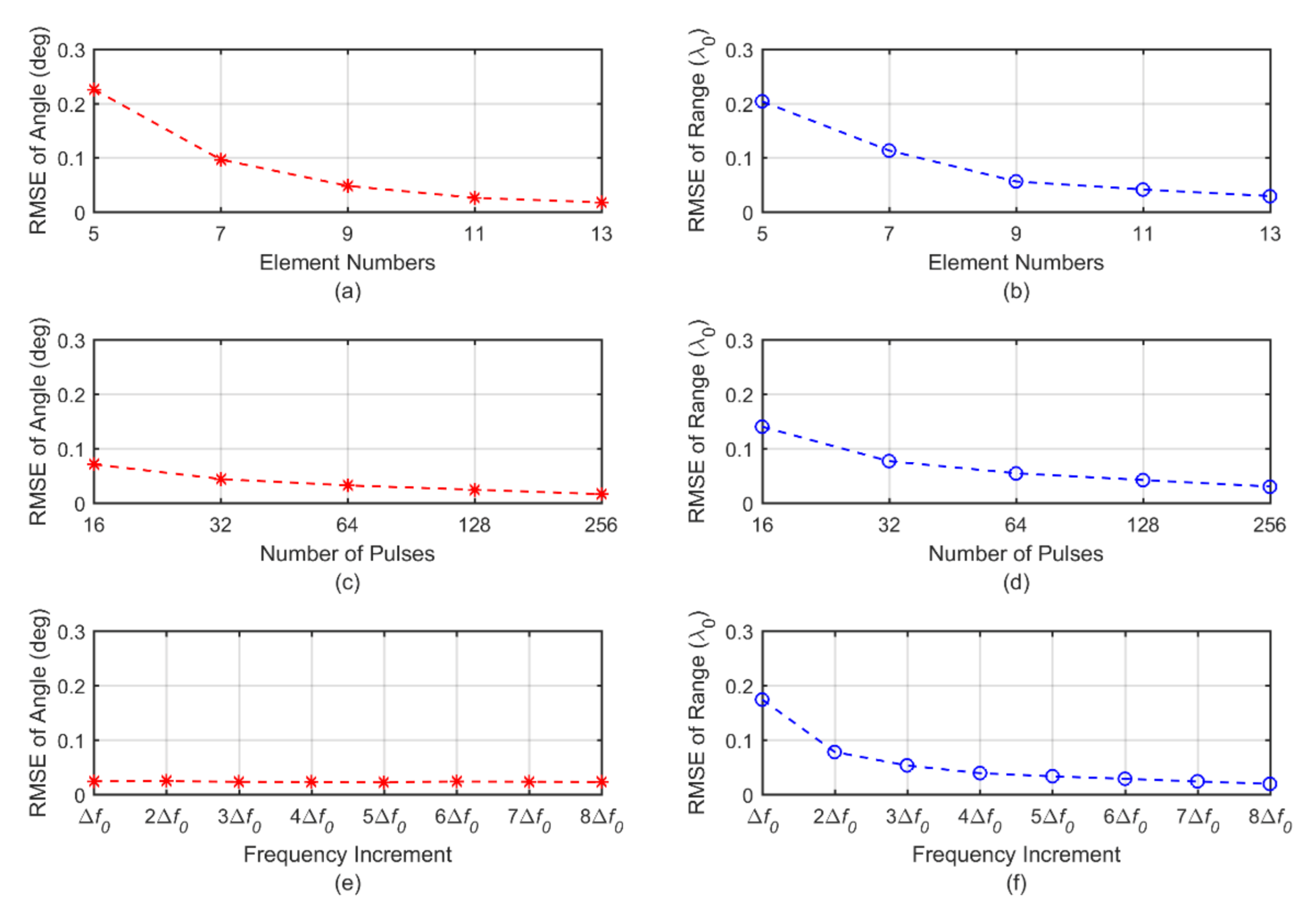
According to the theoretical analysis in Section 3, the estimation of angle and range are sensitive to radar parameters, including the number of array elements N (herein N = 2M + 1), the number of transmitted pulses L, and the frequency increment Δf in the FDA radar. To explore the association between these parameters and estimation performance, the control variable method is utilized in the following experiments.

Figure 4 shows the association between radar parameters and estimation performance, where the red dashed line indicates the RMSE of angle versus the variation in N, L, and Δf, respectively, and the blue dashed line represents the tendency of the RMSE of range. Numerical simulations are conducted by varying one parameter and fixing the other two, and then alternating them. From Figure 4a,b, it is certain that the estimation accuracies of angle and range are enhanced as the array element numbers increase, owing to the diversity gain in the spatial domain. However, increasing element numbers requires greater computational and hardware overhead costs. Similarly, Figure 4c,d show that the estimation performance is improved when the number of pulses is multiple, due to the diversity gain in the time domain. Note that the use of multiple of pulses will lead to huge computational costs; hence, increasing the number of pulses to a high number does not represent an efficient method to pursue performance improvement. Furthermore, the impact of the frequency increment in the FDA is different from the other two parameters. Experiments were conducted by changing the argument of Δf from Δf₀ to seven times Δf₀, in which Δf₀ = 2.5 MHz. From Figure 4e,f, it is clear that the RMSE of angle was independent of the frequency increment, whereas the RMSE of range was sensitive to Δf. This is reasonable since the estimation of range was computed using the range-frequency-dependent terms in the steering vector, while solving angle was unrelated to this argument. It seems that the larger the frequency increment is, the more accurate the estimation of range will be. However, if a larger frequency increment was chosen in the FDA, the fundamental premise of Δf << f₀ was no longer satisfied, leading to the signal model of (8) becoming invalid. Moreover, according to the range constraint defined in (29), the unambiguous range is inversely proportional to the frequency increment. Based on numerical experiments, it is appropriate to set Δf to be around a megahertz for near-field scenarios.

Consequently, in order to achieve better performance as well as to balance the computational cost, it is necessary to make a trade-off regarding the choice of N, L, and Δf.

5.2. Numerical Comparison of the RALS and ALS

Since solving the factor matrices with RALS is an integral part of TenDLA, it is necessary to make a comparison with the ALS algorithm in order to investigate its capacity against the swamp problem, which has a great influence on follow-up procedures. The performance evaluation was conducted with a total of 1500 independent Monte Carlo runs under three types of scenarios. To guarantee fairness and believability, the comparison was conducted using the same input data and factor matrix initialization for every Monte Carlo trial.

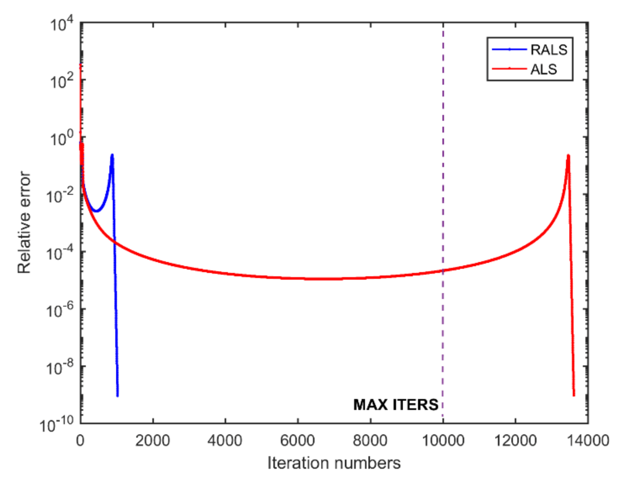
The performance indicators in this comparison are the average number of iterations (AIS), the average computational time (ACT, in seconds), and the ratio of trials above the set maximum iterations (RaMAX). All of the numerical simulations were performed on a desktop computer with an i7-6700 CPU and 16 GB of memory.

Table 3. Performance comparison between RALS and ALS in three scenarios.

Stop Criterion	Algorithms	AIS	ACT	RaMAX (%)
ε = 1 × 10−7	RALS	196	0.2394	0.8
	ALS	222	0.3230	1.4
ε = 1 × 10−8	RALS	207	0.2716	1
	ALS	251	0.400	2.6
ε = 1 × 10−9	RALS	244	0.2915	1.4
	ALS	260	0.3953	2.8

shows the quantitative analysis of the comparison between RALS and ALS. It is clear that RALS outperformed ALS, since it achieved a relatively better performance both on convergence rate and computational cost which is characterized as the AIS of RALS being much lower than that of the ALS algorithm. It is also indicated that RALS can shorten the swamp problem encountered in some ill-conditioned trials to some degree. This is demonstrated in Figure 5 as well, in which RALS effectively shortens the swamp phenomenon with only 1029 iterations compared with the over 13,000 ALS iterations under the condition of encountering an ill-conditioned trial. Furthermore, since the real ALS iteration number in this trial is over the predetermined maximum iteration number, the iterative procedure terminates within the allotted steps whereas the convergence criterion has not been satisfied, leading to a large relative error to solve the CP decomposition and then resulting in performance degradation or incorrect estimation. In contrast, when employing RALS instead of ALS, the number of biased trials can be reduced. The experiment results are consistent with the theoretical analysis in Section 3.2 and demonstrate the superiority of RALS.

5.3. Performance Evaluation of TenDLA

In this section, we compare the performance of different localization techniques via Monte Carlo experiments. Comparisons were made with two existing tensor-based approaches as well as an extensively applied method, including the approximation model based method with the bistatic MIMO radar (Bis-MIMO(AM)) proposed in ref. [33], the corresponding exact model based method (Bis-MIMO(EM)) proposed in ref. [37], and the 2D-MUSIC presented in ref. [7]. To better illustrate performance enhancement via the correction procedure, we also included the estimates achieved using our approach both with correction and without correction.

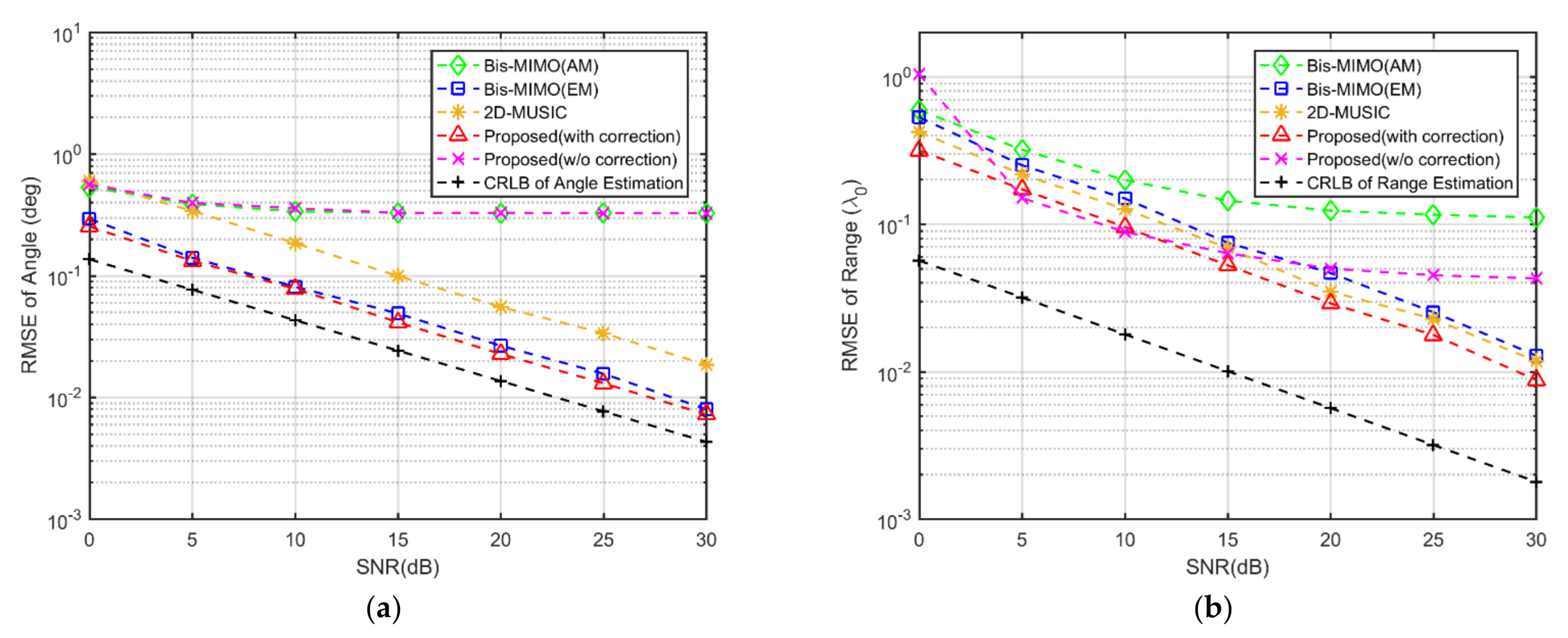
Figure 6a,b show the estimation accuracy versus the SNR. For each SNR value, we conducted 200 independent Monte Carlo runs. From the graphs, we can observe that the proposed approach achieves the most optimal estimation performance for both angle and range compared to the other approaches. On angle estimation, the proposed approach achieved good accuracy that is close to that of Bis-MIMO(EM), and it outperformed the Bis-MIMO(AM) and 2D-MUSIC, demonstrating a significant improvement; in other words, it is possible to achieve comparable estimation accuracy to the exact model based method after angle correction, even if only an approximation model is used. For range estimation, the proposed TenDLA achieved the most optimal resolution compared with the other methods. This can be attributed to the improvement in the spatial resolution by the FDA-MIMO radar and the full exploitation of the signal correlation, which has been discussed in Section 3.2. Additionally, in terms of the comparison between the estimates with correction and without correction in TenDLA, we can clearly observe that the RMSEs of angle and range in the cases with correction decreased as the SNR grew, revealing that the systematic bias caused by the use of the approximation model was mitigated effectively.

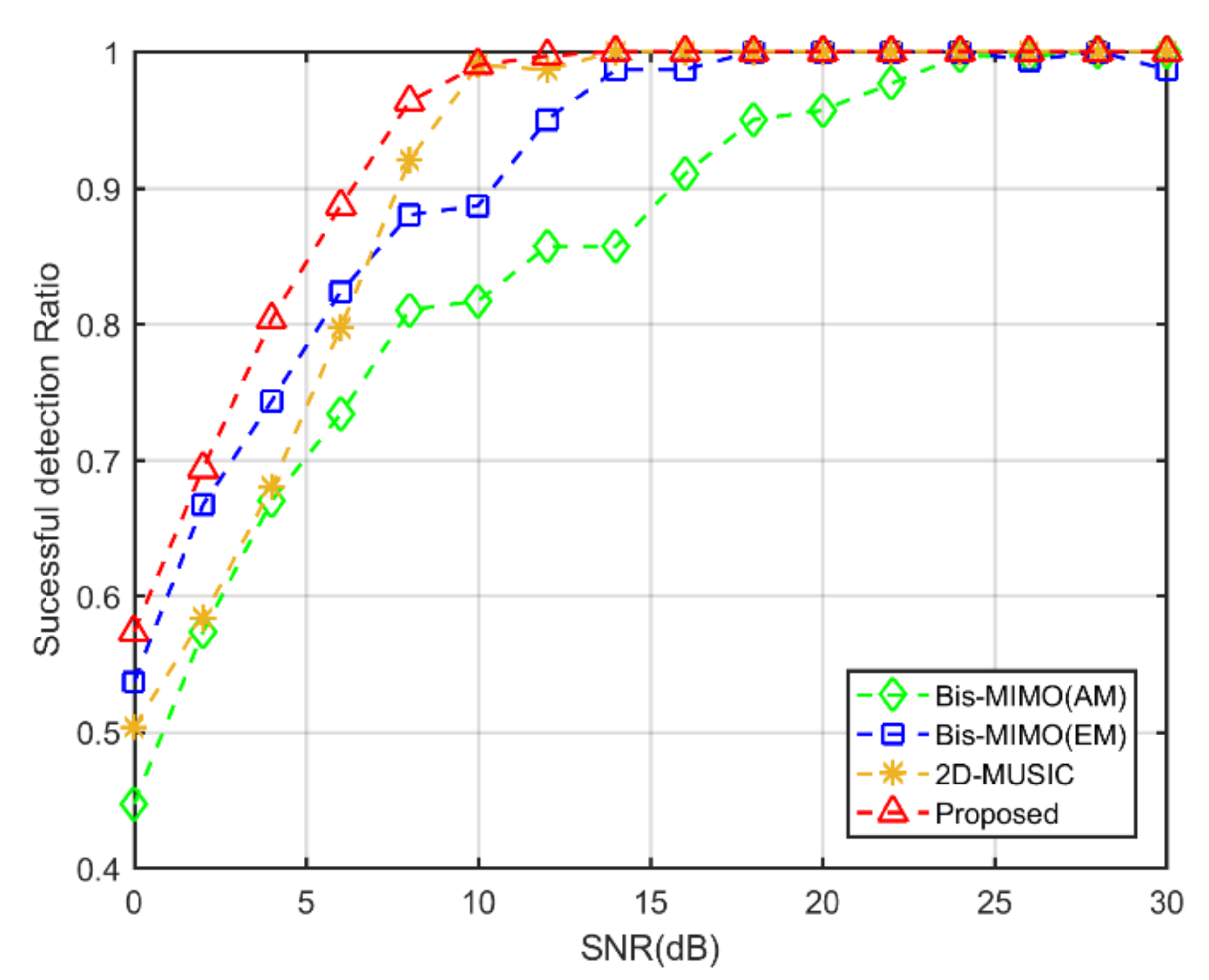
Figure 7 shows the comparison of the successful detection ratio versus the SNR. In this experiment, the parameter settings were the same as they had been previously, and the admitted tolerance for successful detection was determined to be λ/4. On the whole, the successful detection ratio increased as the SNR grew. This makes sense since the estimation accuracy will improve as the noise decreases. Individually, it can be seen from the graph that, although all the methods achieved a high success ratio that was close to 100% in cases where the SNR was high, the proposed approach had a lower SNR threshold compared with other methods. Particularly in low-SNR situations (lower than 10 dB), the proposed method outperformed the other methods, showing improvements of over 10%. It is obvious that the proposed approach is more appropriate in difficult situations than the contrast methods in terms of detection.

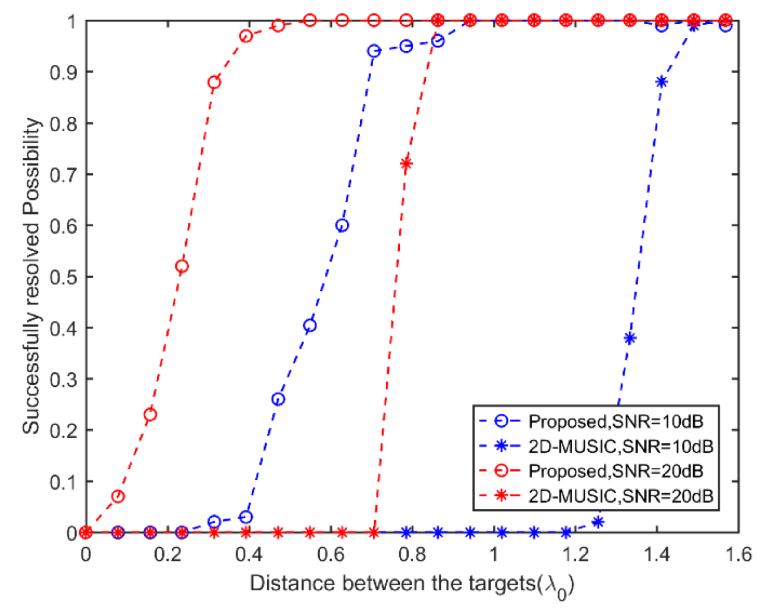
Another prime evaluation indicator is the resolving capability versus the SNR for two closely spaced targets, which can be evaluated via the possibility of the successful detection defined in ref. [37]. We chose the acknowledged super-resolution 2D-MUSIC algorithm as a comparison method. As shown in Figure 8, our proposed method has a much better robust resolution capability than the comparison method; more specifically, it can successfully distinguish two closely spaced targets, even when the distance between the two targets is smaller than half of a wavelength at an SNR of 20 dB and smaller than almost a full wavelength at an SNR of 10 dB.

We also performed a computational cost comparison among different methods. In this experiment, we computed the AIS and ACT by averaging the data obtained during each trial. In terms of AIS, it can be observed from Figure 9 that the proposed approach requires approximately equal iterations to achieve convergence compared to the other two existing tensor-based approaches. This can be verified from the ACT results as well. Since the 2D-MUSIC algorithm requires no iterations, the corresponding computational complexity is indicated by the ACT. Obviously, the computational costs of the proposed approach are much lower than those of the extensively used MUSIC-like algorithm.

5.4. Discussion

The results obtained from various numerical experiments confirmed the effectiveness and robustness of our proposed TenDLA. In conclusion, the attractive advantages of the proposed approach relative to the existing methods are as follows:

1) Improved estimation accuracy: judging from the numerical experiments on estimation accuracy, compared with existing methods, it is clear that TenDLA provides a much better estimation accuracy relative to the recently proposed tensor-based methods, and even outperforms the acknowledged super-resolution algorithm (MUSIC-like algorithms). The systematic biased error encountered in the approximation propagation model based cases was mitigated effectively. Furthermore, the proposed method has a relatively good resolution capability to distinguish two closely spaced targets. The improvement in resolution contributes to the power of tensor-based signal processing and the advantage of FDA-MIMO radar.

2) Simplicity: from the abovementioned numerical experiments on computational cost, we determined that TenDLA has fewer computational costs than conventional spectral searching-based method. This makes sense because the proposed approach is search-free, i.e., the target parameters are resolved via a well-designed strategy that is composed of an algebraic decomposition and a low-cost LS estimation. It does not require taking efforts on multidimensional spectral searching and parameter pairing. Moreover, relative to the existing tensor-based methods, the proposed method has a similar level of complexity. Only a few extra computations are required to fulfill the correction procedures, which are inexpensive and result in improvements in accuracy.

3) Robustness: in some situations, such as the power of the echoes is too low or when two targets are closely spaced, conventional methods (e.g., MUSIC) are usually unable to detect or distinguish the targets clearly. Judging from the results in Figure 6 and Figure 8, it is clear that the proposed method exhibits better performance in difficult situations, both in low-SNR cases and in cases where there are two closely spaced targets. Additionally, when calculating the CP decomposition encountering ill-conditioned cases, the TenDLA offers the capacity to shorten the swamp problem relative to the conventional ALS-based approach, making it possible to gain improvement in numerical stability.

6. Conclusions

In this paper, a tensor decomposition-based localization algorithm (TenDLA) for near-field multiple targets with a symmetric monostatic FDA-MIMO radar was proposed. In the TenDLA, the joint range and angle estimation was resolved by converting the target localization into the problem of solving the tensor decomposition. Benefiting from the introduced RALS algorithm, the reliability on numerical calculation is enhanced evidently. Additionally, the improved solution on the joint range and angle estimation proposed in this work can mitigate the systematic biased errors with limited extra correction procedures, yielding a significant improvement in estimation accuracy. Numerical experiments illustrate the validity and accuracy of the proposed approach, and it showcases its potential in applications for detecting and sensing near-field multiple targets in a variety of fields.

References

1. Godrich, H.; Haimovich, A.M.; Blum, R.S. Target Localization Accuracy Gain in MIMO Radar-Based Systems. IEEE Trans. Inf. Theory 2010, 56, 2783–2803. [Google Scholar] [CrossRef]
2. Bilik, I.; Longman, O.; Villeval, S.; Tabrikian, J. The Rise of Radar for Autonomous Vehicles: Signal Processing Solutions and Future Research Directions. IEEE Signal Process. Mag. 2019, 36, 20–31. [Google Scholar] [CrossRef]
3. Konno, K.; Honma, N.; Sasakawa, D.; Tsunekawa, Y.; Nishimori, K.; Takemura, N.; Mitsui, T. Localizing Multiple Target Using Bistatic MIMO Radar in Multi-Path Environment. In Proceedings of the 2014 IEEE International Workshop on Electromagnetics (iWEM), Sapporo, Japan, 4–6 August 2014; pp. 90–91. [Google Scholar]
4. Rascon, C.; Meza, I. Localization of Sound Sources in Robotics: A Review. Robot. Auton. Syst. 2017, 96, 184–210. [Google Scholar] [CrossRef]
5. Zeng, Z.; Li, J.; Huang, L.; Feng, X.; Liu, F. Improving Target Detection Accuracy Based on Multipolarization MIMO GPR. IEEE Trans. Geosci. Remote Sens. 2015, 53, 15–24. [Google Scholar] [CrossRef]
6. Huang, Y.-D.; Barkat, M. Near-Field Multiple Source Localization by Passive Sensor Array. IEEE Trans. Antennas Propag. 1991, 39, 968–975. [Google Scholar] [CrossRef]
7. Krim, H.; Viberg, M. Two Decades of Array Signal Processing Research: The Parametric Approach. IEEE Signal Process. Mag. 1996, 13, 67–94. [Google Scholar] [CrossRef]
8. Zhi, W.; Chia, M.Y.-W. Near-Field Source Localization via Symmetric Subarrays. IEEE Signal Process. Lett. 2007, 14, 409–412. [Google Scholar] [CrossRef]
9. Chen, J.C.; Hudson, R.E.; Yao, K. Maximum-Likelihood Source Localization and Unknown Sensor Location Estimation for Wideband Signals in the near-Field. IEEE Trans. Signal Process. 2002, 50, 1843–1854. [Google Scholar] [CrossRef]
10. Grosicki, E.; Abed-Meraim, K.; Hua, Y. A Weighted Linear Prediction Method for Near-Field Source Localization. IEEE Trans. Signal Process. 2005, 53, 3651–3660. [Google Scholar] [CrossRef]
11. Zuo, W.; Xin, J.; Ohmori, H.; Zheng, N.; Sano, A. Subspace-Based Algorithms for Localization and Tracking of Multiple Near-Field Sources. IEEE J. Sel. Top. Signal Process. 2019, 13, 156–171. [Google Scholar] [CrossRef]
12. Zheng, Z.; Fu, M.; Wang, W.-Q.; Zhang, S.; Liao, Y. Localization of Mixed Near-Field and Far-Field Sources Using Symmetric Double-Nested Arrays. IEEE Trans. Antennas Propag. 2019, 67, 7059–7070. [Google Scholar] [CrossRef]
13. Yuen, N.; Friedlander, B. Performance Analysis of Higher Order ESPRIT for Localization of Near-Field Sources. IEEE Trans. Signal Process. 1998, 46, 709–719. [Google Scholar] [CrossRef]
14. Li, J.; Stoica, P. MIMO Radar with Colocated Antennas. IEEE Signal Process. Mag. 2007, 24, 106–114. [Google Scholar] [CrossRef]
15. Antonik, P.; Wicks, M.C.; Griffiths, H.D.; Baker, C.J. Frequency Diverse Array Radars. In Proceedings of the 2006 IEEE Conference on Radar, Syracuse, NY, USA, 24–27 April 2006; pp. 215–217. [Google Scholar]
16. Wang, W. Overview of Frequency Diverse Array in Radar and Navigation Applications. IET Radar Sonar Navig. 2016, 10, 1001–1012. [Google Scholar] [CrossRef]
17. Wang, W.-Q.; So, H.C.; Farina, A. An Overview on Time/Frequency Modulated Array Processing. IEEE J. Sel. Top. Signal Process. 2017, 11, 228–246. [Google Scholar] [CrossRef]
18. Xu, J.; Liao, G.; Zhu, S.; Huang, L.; So, H.C. Joint Range and Angle Estimation Using MIMO Radar With Frequency Diverse Array. IEEE Trans. Signal Process. 2015, 63, 3396–3410. [Google Scholar] [CrossRef]
19. Cui, C.; Xu, J.; Gui, R.; Wang, W.-Q.; Wu, W. Search-Free DOD, DOA and Range Estimation for Bistatic FDA-MIMO Radar. IEEE Access 2018, 6, 15431–15445. [Google Scholar] [CrossRef]
20. Xiong, J.; Wang, W.-Q.; Gao, K. FDA-MIMO Radar Range–Angle Estimation: CRLB, MSE, and Resolution Analysis. IEEE Trans. Aerosp. Electron. Syst. 2018, 54, 284–294. [Google Scholar] [CrossRef]
21. Sammartino, P.F.; Baker, C.J.; Griffiths, H.D. Frequency Diverse MIMO Techniques for Radar. IEEE Trans. Aerosp. Electron. Syst. 2013, 49, 201–222. [Google Scholar] [CrossRef]
22. Chen, H.; Ahmad, F.; Vorobyov, S.; Porikli, F. Tensor Decompositions in Wireless Communications and MIMO Radar. IEEE J. Sel. Top. Signal Process. 2021, 15, 438–453. [Google Scholar] [CrossRef]
23. Cichocki, A.; Mandic, D.; De Lathauwer, L.; Zhou, G.; Zhao, Q.; Caiafa, C.; Phan, H.A. Tensor Decompositions for Signal Processing Applications: From Two-Way to Multiway Component Analysis. IEEE Signal Process. Mag. 2015, 32, 145–163. [Google Scholar] [CrossRef]
24. Kolda, T.G.; Bader, B.W. Tensor Decompositions and Applications. SIAM Rev. 2009, 51, 455–500. [Google Scholar] [CrossRef]
25. Sidiropoulos, N.D.; De Lathauwer, L.; Fu, X.; Huang, K.; Papalexakis, E.E.; Faloutsos, C. Tensor Decomposition for Signal Processing and Machine Learning. IEEE Trans. Signal Process. 2017, 65, 3551–3582. [Google Scholar] [CrossRef]
26. Kruskal, J.B. Three-Way Arrays: Rank and Uniqueness of Trilinear Decompositions, with Application to Arithmetic Complexity and Statistics. Linear Algebra Appl. 1977, 18, 95–138. [Google Scholar] [CrossRef]
27. Nion, D.; Sidiropoulos, N.D. Tensor Algebra and Multidimensional Harmonic Retrieval in Signal Processing for MIMO Radar. IEEE Trans. Signal Process. 2010, 58, 5693–5705. [Google Scholar] [CrossRef]
28. Nion, D.; Sidiropoulos, N.D. A PARAFAC-Based Technique for Detection and Localization of Multiple Targets in a MIMO Radar System. In Proceedings of the 2009 IEEE International Conference on Acoustics, Speech and Signal Processing, Taipei, Taiwan, 19–24 April 2009; pp. 2077–2080. [Google Scholar]
29. Zhang, X.; Xu, Z.; Xu, L.; Xu, D. Trilinear Decomposition-Based Transmit Angle and Receive Angle Estimation for Multiple-Input Multiple-Output Radar. IET Radar Sonar Navig. 2011, 5, 626–631. [Google Scholar] [CrossRef]
30. Li, J.; Zhou, M. Improved Trilinear Decomposition-based Method for Angle Estimation in Multiple-input Multiple-output Radar. IET Radar Sonar Navig. 2013, 7, 1019–1026. [Google Scholar] [CrossRef]
31. Xu, B.; Zhao, Y.; Cheng, Z.; Li, H. A Novel Unitary PARAFAC Method for DOD and DOA Estimation in Bistatic MIMO Radar. Signal Process. 2017, 138, 273–279. [Google Scholar] [CrossRef]
32. Wang, X.; Wang, W.; Liu, J.; Liu, Q.; Wang, B. Tensor-Based Real-Valued Subspace Approach for Angle Estimation in Bistatic MIMO Radar with Unknown Mutual Coupling. Signal Process. 2015, 116, 152–158. [Google Scholar] [CrossRef]
33. Singh, P.R.; Wang, Y.; Chargé, P. Bistatic MIMO Radar for near Field Source Localisation Using PARAFAC. Electron. Lett. 2016, 52, 1060–1061. [Google Scholar] [CrossRef]
34. Hsu, Y.-S.; Wong, K.T.; Yeh, L. Mismatch of Near-Field Bearing-Range Spatial Geometry in Source-Localization by a Uniform Linear Array. IEEE Trans. Antennas Propag. 2011, 59, 3658–3667. [Google Scholar] [CrossRef]
35. Singh, P.R.; Wang, Y.; Chargé, P. A Correction Method for the near Field Approximated Model Based Localization Techniques. Digit. Signal Process. 2017, 67, 76–80. [Google Scholar] [CrossRef]
36. Podkurkov, I.; Seidl, G.; Khamidullina, L.; Nadeev, A.; Haardt, M. Tensor-Based Near-Field Localization Using Massive Antenna Arrays. IEEE Trans. Signal Process. 2021, 69, 5830–5845. [Google Scholar] [CrossRef]
37. Singh, P.; Wang, Y.; Chargé, P. An Exact Model-Based Method for Near-Field Sources Localization with Bistatic MIMO System. Sensors 2017, 17, 723. [Google Scholar] [CrossRef]
38. Sherman, J. Properties of Focused Apertures in the Fresnel Region. IRE Trans. Antennas Propag. 1962, 10, 399–408. [Google Scholar] [CrossRef]
39. Swerling, P. Probability of Detection for Fluctuating Targets. IEEE Trans. Inf. Theory 1960, 6, 269–308. [Google Scholar] [CrossRef]
40. Navasca, C.; De Lathauwer, L.; Kindermann, S. Swamp Reducing Technique for Tensor Decomposition. In Proceedings of the 2008 16th European Signal Processing Conference, Lausanne, Switzerland, 25–29 August 2008; pp. 1–5. [Google Scholar]
41. Li, N.; Kindermann, S.; Navasca, C. Some Convergence Results on the Regularized Alternating Least-Squares Method for Tensor Decomposition. Linear Algebra Appl. 2013, 438, 796–812. [Google Scholar] [CrossRef]
42. Zhang, X. Matrix Analysis and Applications, 2nd ed.; Tsinghua University Press: Beijing, China, 2013; pp. 596–609. [Google Scholar]
43. Hu, K.; Chepuri, S.P.; Leus, G. Near-Field Source Localization: Sparse Recovery Techniques and Grid Matching. In Proceedings of the 2014 IEEE 8th Sensor Array and Multichannel Signal Processing Workshop (SAM), A Coruna, Spain, 22–25 June 2014; pp. 369–372. [Google Scholar]
44. Zhou, E.; Jiang, H.; Qi, H. 4-D parameter estimation in bistatic MIMO radar for near-field target localization. In Proceedings of the 2015 IEEE International Wireless Symposium (IWS 2015), Shenzhen, China, 30 March–1 April 2015; pp. 1–4. [Google Scholar]
45. Xu, J.; Zhu, S.; Liao, G.; Zhang, Y. An overview of frequency diverse array radar technology. J. Radars 2018, 7, 167–182. [Google Scholar] [CrossRef]
Figure 1. The structure of the FDA−MIMO radar.
Remotesensing 14 04392 g001
Figure 2. Block diagram of echo data conversion processing.
Remotesensing 14 04392 g002
Figure 3. The basic flow of target localization based on tensor decomposition.
Remotesensing 14 04392 g003
Figure 4. The impact on estimation performance in terms of radar parameters. (a) RMSE of angle versus element numbers; (b) RMSE of range versus element numbers; (c) RMSE of angle versus number of pulses; (d) RMSE of range versus number of pulses; (e) RMSE of angle versus frequency increment; (f) RMSE of range versus frequency increment.
Remotesensing 14 04392 g004
Figure 5. Comparison of convergence rate between RALS and ALS in one ill−conditioned trial.
Remotesensing 14 04392 g005
Figure 6. Comparison of estimation performance versus SNR. (a) RMSE of angle versus SNR, (b) RMSE of range versus SNR.
Remotesensing 14 04392 g006
Figure 7. Comparison of successful detection ratio versus SNR.
Remotesensing 14 04392 g007
Figure 8. Resolution threshold versus SNR for two closely spaced targets.
Remotesensing 14 04392 g008
Figure 9. Comparison of AIS and ACT.
Remotesensing 14 04392 g009