
DGPolarNet: Dynamic Graph Convolution Network for LiDAR Point Cloud Semantic Segmentation on Polar BEV


Abstract
:1. Introduction
2. Related Works
2.1. Multiview Projection Methods
2.2. Voxelization Methods
2.3. Point Methods
2.4. Graph Methods
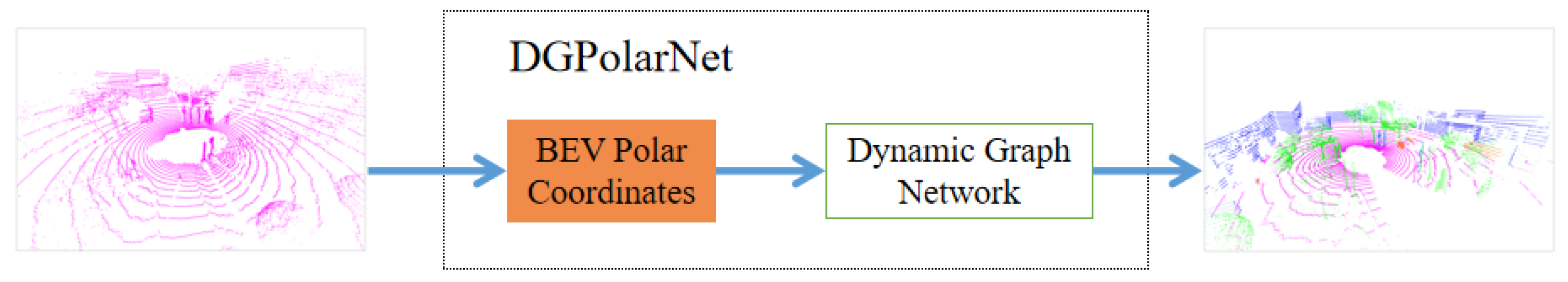
3. DGPolarNet for LiDAR Point Cloud Semantic Segmentation
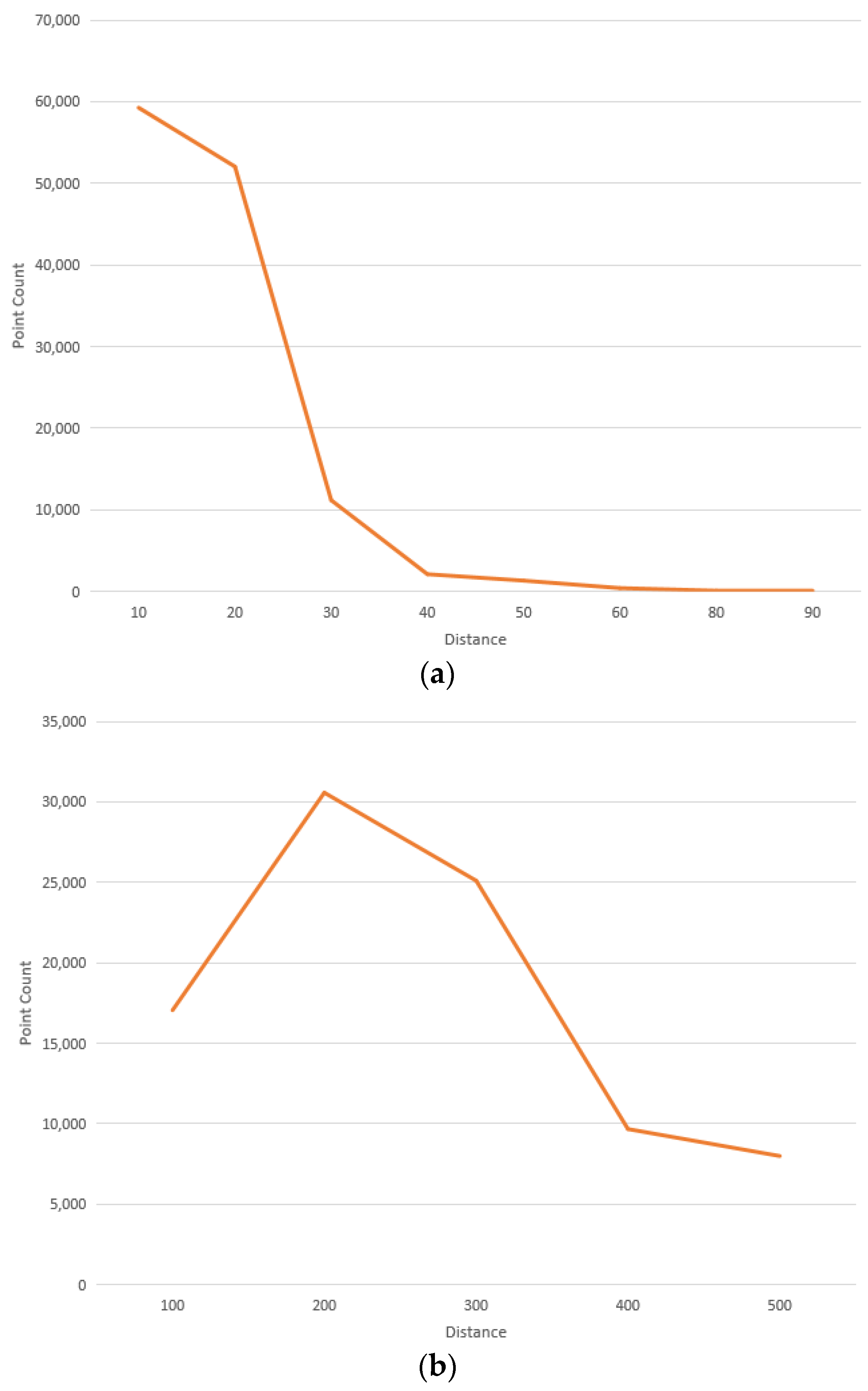
3.1. BEV Polar Converter
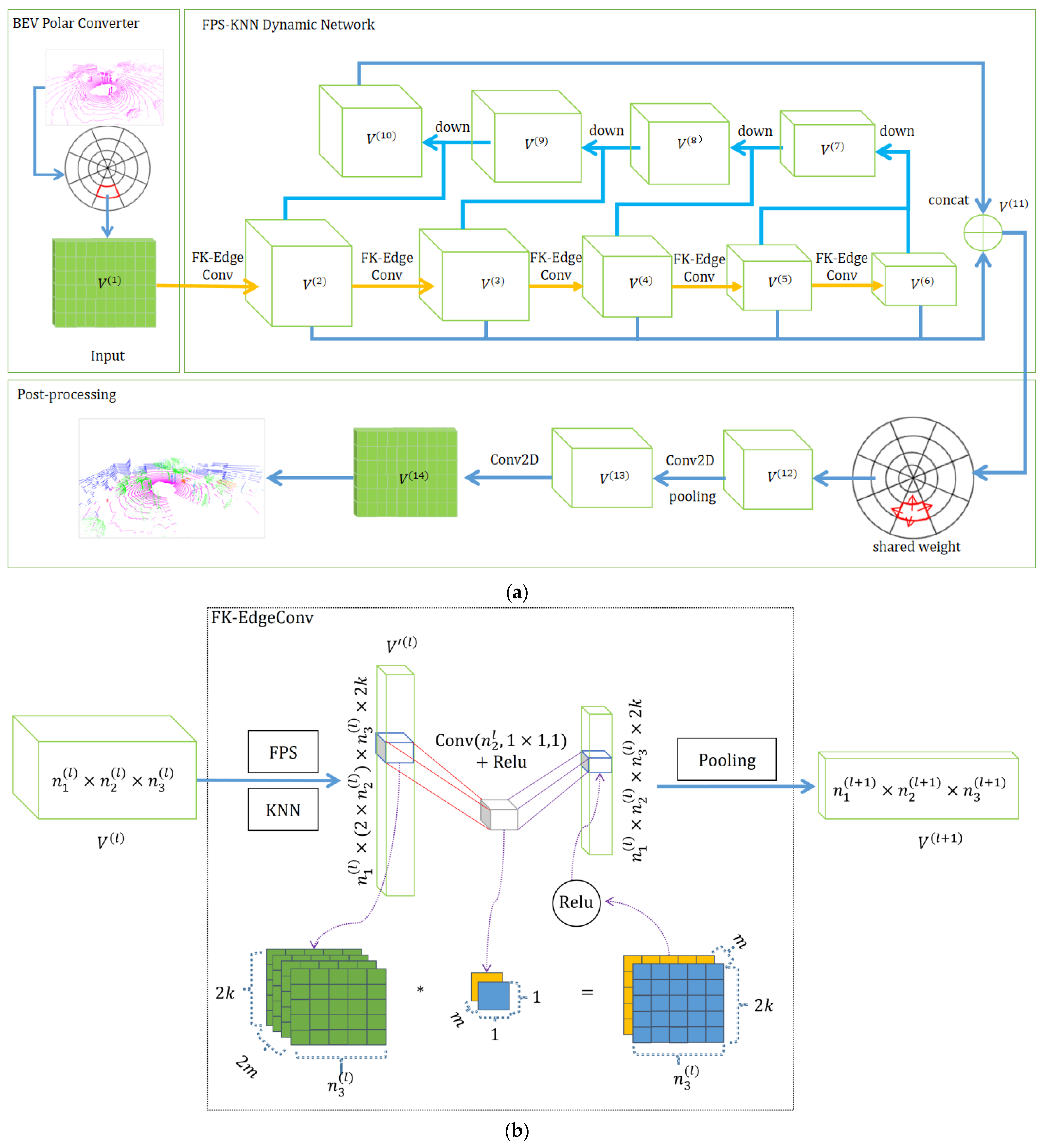
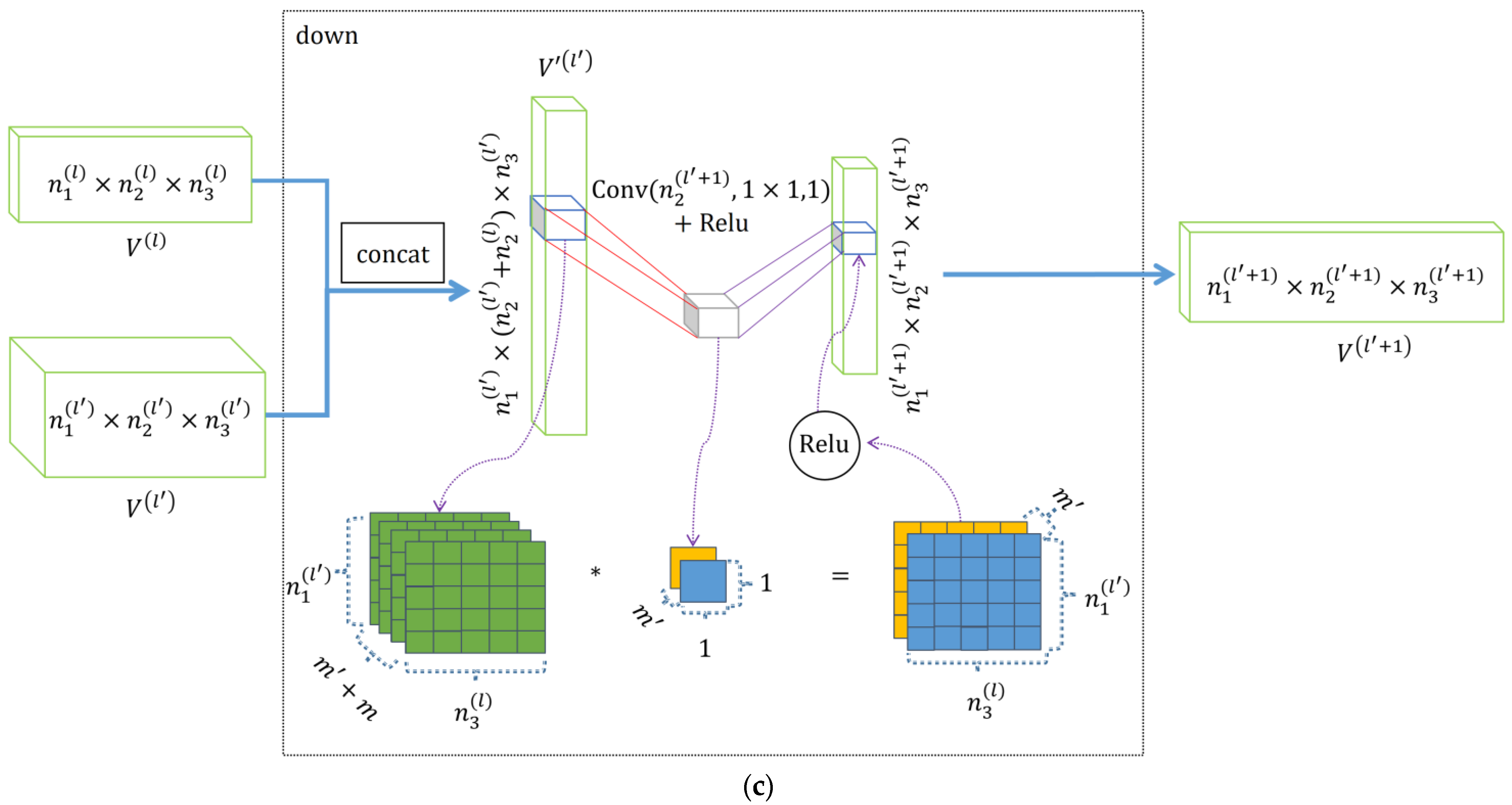
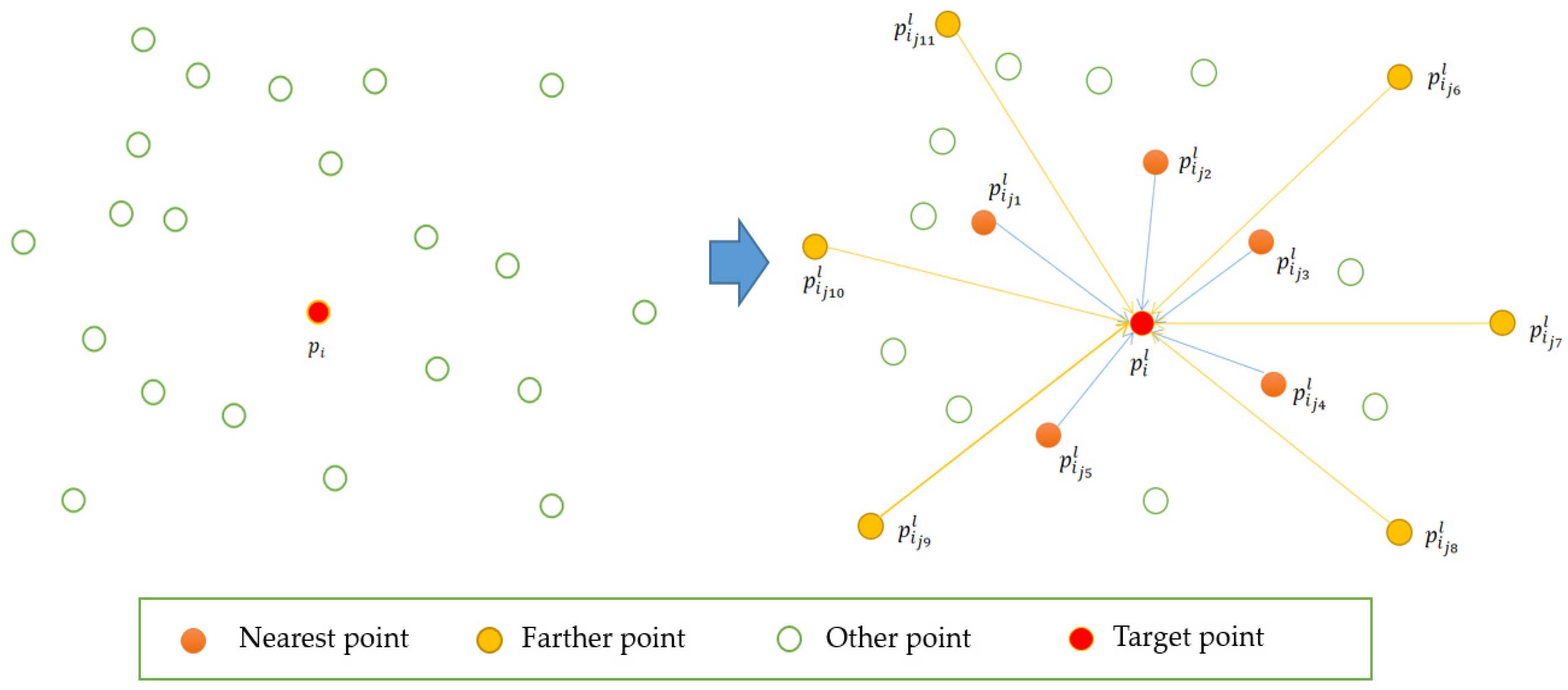
3.2. FPS-KNN Dynamic Network
3.3. Postprocessing
4. Experiments and Analysis
4.1. Datasets
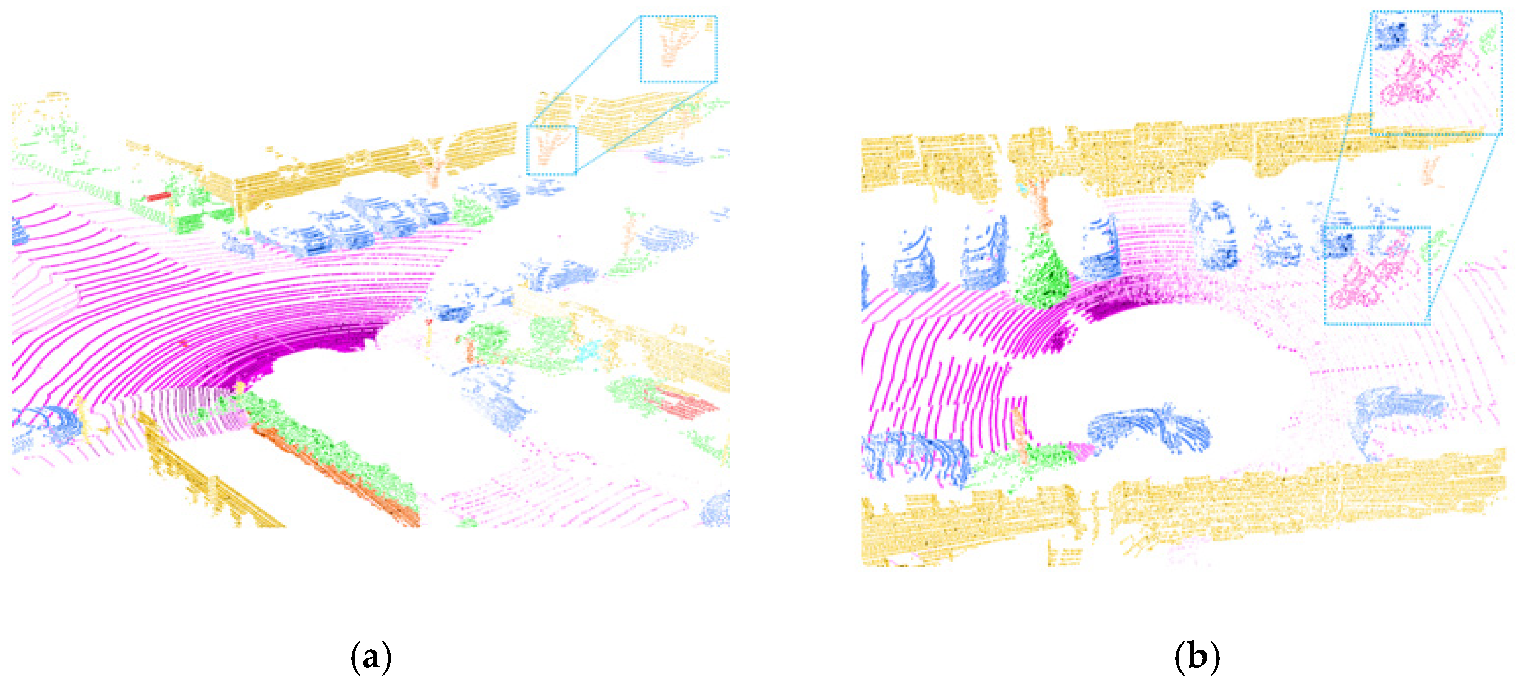
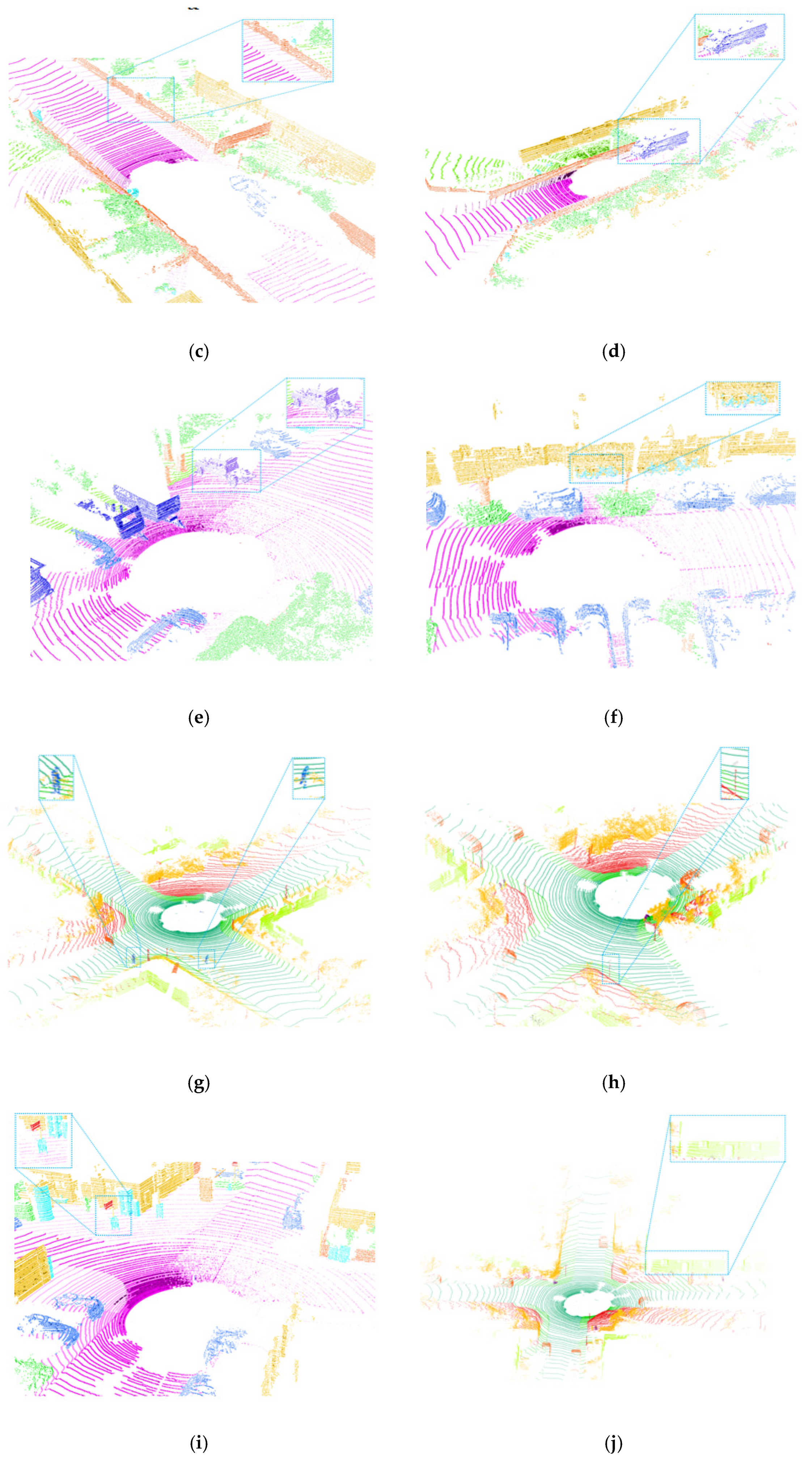
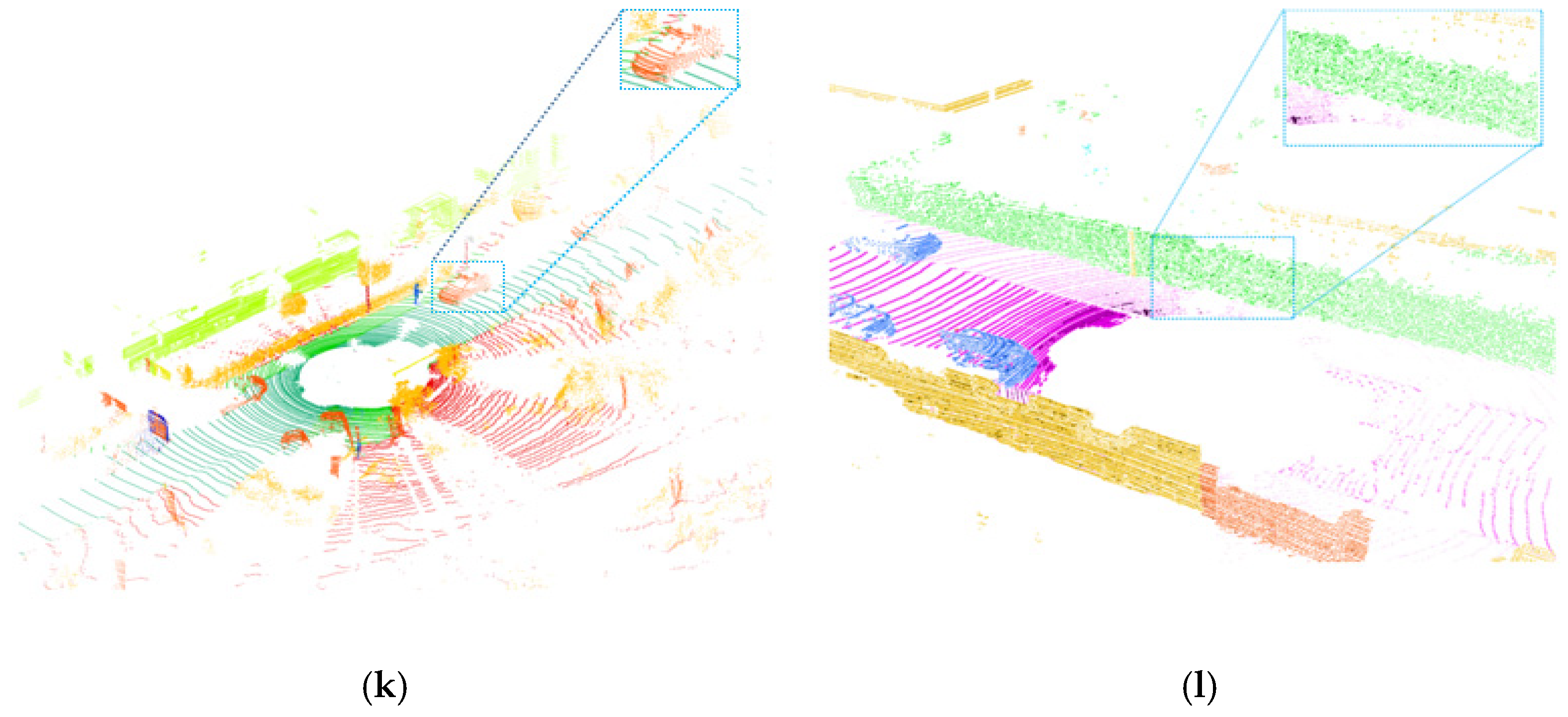
4.2. Semantic Segmentation Performance
5. Conclusions
Author Contributions
Funding
Data Availability Statement
Conflicts of Interest
References
- Ballouch, Z.; Hajji, R.; Poux, F.; Kharroubi, A.; Billen, R. A Prior Level Fusion Approach for the Semantic Segmentation of 3D Point Clouds Using Deep Learning. Remote Sens. 2022, 14, 3415. [Google Scholar] [CrossRef]
- Wei, M.; Zhu, M.; Zhang, Y.; Sun, J.; Wang, J. Cyclic Global Guiding Network for Point Cloud Completion. Remote Sens. 2022, 14, 3316. [Google Scholar] [CrossRef]
- Song, W.; Li, D.; Sun, S.; Zhang, L.; Xin, Y.; Sung, Y.; Choi, R. 2D&3DHNet for 3D Object Classification in LiDAR Point Cloud. Remote Sens. 2022, 14, 3146. [Google Scholar] [CrossRef]
- Decker, K.T.; Borghetti, B.J. Composite Style Pixel and Point Convolution-Based Deep Fusion Neural Network Architecture for the Semantic Segmentation of Hyperspectral and Lidar Data. Remote Sens. 2022, 14, 2113. [Google Scholar] [CrossRef]
- Liu, R.; Tao, F.; Liu, X.; Na, J.; Leng, H.; Wu, J.; Zhou, T. RAANet: A Residual ASPP with Attention Framework for Semantic Segmentation of High-Resolution Remote Sensing Images. Remote Sens. 2022, 14, 3109. [Google Scholar] [CrossRef]
- Xu, T.; Gao, X.; Yang, Y.; Xu, L.; Xu, J.; Wang, Y. Construction of a Semantic Segmentation Network for the Overhead Catenary System Point Cloud Based on Multi-Scale Feature Fusion. Remote Sens. 2022, 14, 2768. [Google Scholar] [CrossRef]
- Shuang, F.; Li, P.; Li, Y.; Zhang, Z.; Li, X. MSIDA-Net: Point Cloud Semantic Segmentation via Multi-Spatial Information and Dual Adaptive Blocks. Remote Sens. 2022, 14, 2187. [Google Scholar] [CrossRef]
- Eeinmann, M.; Jutzi, B.; Hinz, S.; Mallet, C. Semantic point cloud interpretation based on optimal neighborhoods, relevant features and efficient classifiers. ISPRS J. Photogramm. Remote Sens. 2015, 105, 286–304. [Google Scholar] [CrossRef]
- Zhang, Y.; Zhou, Z.; David, P.; Yue, X.; Xi, Z.; Gong, B.; Foroosh, H. PolarNet: An Improved Grid Representation for Online LiDAR Point Clouds Semantic Segmentation. In Proceedings of the 2020 IEEE/CVF Conference on Computer Vision and Pattern Recognition (CVPR), Seattle, WA, USA, 13–19 June 2020; pp. 9598–9607. [Google Scholar]
- Lawin, F.J.; Danelljan, M.; Tosteberg, P.; Bhat, G.; Khan, F.S.; Felsberg, M. Deep Projective 3D Semantic Segmentation. In Proceedings of the Computer Analysis of Images and Patterns, Ystad, Sweden, 22–24 August 2017; pp. 55–107. [Google Scholar]
- Boulch, A.; Saux, B.L.; Audebert, N. Unstructured point cloud semantic labeling using deep segmentation networks. In Proceedings of the Workshop on 3D Object Retrieval (3Dor ‘17). Eurographics Association, Goslar, Germany, 23 April 2017; pp. 17–24. [Google Scholar]
- Tatarchenko, M.; Park, J.; Koltun, V.; Zhou, Q.-Y. Tangent Convolutions for Dense Prediction in 3D. In Proceedings of the 2018 IEEE/CVF Conference on Computer Vision and Pattern Recognition, Salt Lake City, UT, USA, 18–23 June 2018; pp. 3887–3896. [Google Scholar]
- Su, H.; Jampani, V.; Sun, D.; Maji, S.; Kalogerakis, E.; Yang, M.H.; Kautz, J. SPLATNet: Sparse Lattice Networks for Point Cloud Processing. In Proceedings of the 2018 IEEE/CVF Conference on Computer Vision and Pattern Recognition, Salt Lake City, UT, USA, 18–23 June 2018; pp. 2530–2539. [Google Scholar]
- Wu, B.; Wan, A.; Yue, X.; Keutzer, K. SqueezeSeg: Convolutional Neural Nets with Recurrent CRF for Real-Time Road-Object Segmentation from 3D LiDAR Point Cloud. In Proceedings of the 2018 IEEE International Conference on Robotics and Automation (ICRA), Brisbane, Australia, 21–25 May 2018; pp. 1887–1893. [Google Scholar]
- Milioto, A.; Stachniss, C. RangeNet ++: Fast and Accurate LiDAR Semantic Segmentation. In Proceedings of the 2019 IEEE/RSJ International Conference on Intelligent Robots and Systems (IROS), Macau, China, 3–8 November 2019; pp. 4213–4220. [Google Scholar]
- Su, H.; Maji, S.; Kalogerakis, E.; Learned-Miller, E. Multi-view Convolutional Neural Networks for 3D Shape Recognition. In Proceedings of the 2015 IEEE International Conference on Computer Vision (ICCV), Santiago, Chile, 7–13 December 2015; pp. 945–953. [Google Scholar]
- Feng, Y.; Zhang, Z.; Zhao, X.; Ji, R.; Gao, Y. GVCNN: Group-View Convolutional Neural Networks for 3D Shape Recognition. In Proceedings of the 2018 IEEE/CVF Conference on Computer Vision and Pattern Recognition, Salt Lake City, UT, USA, 18–23 June 2018; pp. 264–272. [Google Scholar]
- Wang, C.; Pelillo, M.; Siddiqi, K. Dominant set clustering and pooling for multi-view 3D object recognition. In Proceedings of the British Machine Vision Conference 2017, London, UK, 4–7 September 2017; pp. 1–12. [Google Scholar]
- Ma, C.; Guo, Y.; Yang, J.; An, W. Learning Multi-View Representation with LSTM for 3-D Shape Recognition and Retrieval. IEEE Trans. Multimed. 2019, 21, 1169–1182. [Google Scholar] [CrossRef]
- Maturana, D.; Scherer, S. VoxNet: A 3D Convolutional Neural Network for real-time object recognition. In Proceedings of the 2015 IEEE/RSJ International Conference on Intelligent Robots and Systems (IROS), Hamburg, Germany, 28 September–3 October 2015; pp. 922–928. [Google Scholar]
- Rethage, D.; Wald, J.; Sturm, J.; Navab, N.; Tombari, F. Fully-Convolutional Point Networks for Large-Scale Point Clouds. In Proceedings of the European Conference on Computer Vision ECCV 2018, Munich, Germany, 8–14 September 2018; pp. 596–611. [Google Scholar]
- Graham, B.; Engelcke, M.; Maaten, L. 3D Semantic Segmentation with Submanifold Sparse Convolutional Networks. In Proceedings of the 2018 IEEE/CVF Conference on Computer Vision and Pattern Recognition, Salt Lake City, UT, USA, 18–23 June 2018; pp. 9224–9232. [Google Scholar]
- Wu, Z.; Song, S.; Khosla, A.; Yu, F.; Zhang, L.; Tang, X.; Xiao, J. 3D ShapeNets: A deep representation for volumetric shapes. In Proceedings of the 2015 IEEE Conference on Computer Vision and Pattern Recognition (CVPR), Boston, MA, USA, 7–12 June 2015; pp. 1912–1920. [Google Scholar]
- Riegler, G.; Ulusoy, A.O.; Geiger, A. OctNet: Learning Deep 3D Representations at High Resolutions. In Proceedings of the 2017 IEEE Conference on Computer Vision and Pattern Recognition (CVPR), Honolulu, HI, USA, 21–26 July 2017; pp. 6620–6629. [Google Scholar]
- Wang, P.S.; Liu, Y.X.; Guo, Y.X.; Sun, C.Y.; Tong, X. O-CNN: Octree-based Convolutional Neural Networks for 3D Shape Analysis. ACM Trans. Graph. 2017, 36, 1–11. [Google Scholar] [CrossRef]
- Xu, Y.; Hoegner, L.; Tuttas, S.; Stilla, U. Voxel- and Graph-based Point Cloud Segmentation of 3D Scenes Using Perceptual Grouping Laws. In Proceedings of the ISPRS Annals of Photogrammetry, Remote Sensing and Spatial Information Sciences, Boston, MA, USA, 7–12 June 2017; pp. 43–50. [Google Scholar]
- Li, Y.Y.; Pirk, S.; Su, H.; Qi, C.R.; Guibas, L.J. FPNN: Field Probing Neural Networks for 3D Data. In Proceedings of the NIPS’16: Proceedings of the 30th International Conference on Nrural Information Processing Systems, Barcelona, Spain, 5–10 December 2016; pp. 207–315. [Google Scholar]
- Le, T.; Duan, Y. PointGrid: A Deep Network for 3D Shape Understanding. In Proceedings of the 2018 IEEE/CVF Conference on Computer Vision and Pattern Recognition, Salt Lake City, UT, USA, 18–23 June 2018; pp. 9204–9214. [Google Scholar]
- Tchapmi, L.; Choy, C.; Armeni, I.; Gwak, J.; Savarese, S. SEGCloud: Semantic Segmentation of 3D Point Clouds. In Proceedings of the 2017 International Conference on 3D Vision (3DV), Qingdao, China, 10–12 October 2017; pp. 537–547. [Google Scholar]
- Qi, C.; Su, H.; Mo, K.; Guibas, L.J. PointNet: Deep Learning on Point Sets for 3D Classification and Segmentation. In Proceedings of the 2017 IEEE Conference on Computer Vision and Pattern Recognition (CVPR), Honolulu, HI, USA, 21–26 July 2017; pp. 77–85. [Google Scholar]
- Qi, C.R.; Yi, L.; Su, H.; Guibas, L.J. Pointnet++: Deep hierarchical feature learning on point sets in a metric space. In Proceedings of the NIPS’17: Proceedings of the 31st International Conference on Neural Information Processing Systems, Long Beach, CA, USA, 4–9 December 2017; Curran Associates Inc.: Red Hook, NY, USA, 2017; pp. 5105–5114. [Google Scholar]
- Jiang, M.; Wu, Y.; Zhao, T.; Zhao, Z.; Lu, C. PointSIFT: A SIFT-like Network Module for 3D Point Cloud Semantic Segmentation. arXiv 2018, arXiv:1807.00652. [Google Scholar]
- Li, J.; Chen, B.M.; Lee, G.H. SO-Net: Self-Organizing Network for Point Cloud Analysis. In Proceedings of the 2018 IEEE/CVF Conference on Computer Vision and Pattern Recognition, Salt Lake City, UT, USA, 18–23 June 2018; pp. 9397–9406. [Google Scholar]
- Wang, Y.; Chao, W.; Garg, D.; Hariharan, B.; Campbell, M.; Weinberger, K. Pseudo-LiDAR From Visual Depth Estimation: Bridging the Gap in 3D Object Detection for Autonomous Driving. In Proceedings of the 2019 IEEE/CVF Conference on Computer Vision and Pattern Recognition (CVPR), Long Beach, CA, USA, 15–20 June 2019; pp. 8437–8445. [Google Scholar]
- Yang, B.; Luo, W.; Urtasun, R. PIXOR: Real-time 3D Object Detection from Point Clouds. In Proceedings of the 2018 IEEE/CVF Conference on Computer Vision and Pattern Recognition, Salt Lake City, UT, USA, 18–23 June 2018; pp. 7652–7660. [Google Scholar]
- Lang, A.H.; Vora, S.; Caesar, H.; Zhou, L.; Yang, J.; Beijbom, O. PointPillars: Fast Encoders for Object Detection From Point Clouds. In Proceedings of the 2019 IEEE/CVF Conference on Computer Vision and Pattern Recognition (CVPR), Long Beach, CA, USA, 15–20 June 2019; pp. 8437–8445. [Google Scholar]
- Ku, J.; Mozififian, M.; Lee, J.; Harakeh, A.; Waslander, S.L. Joint 3D Proposal Generation and Object Detection from View Aggregation. In Proceedings of the 2018 IEEE/RSJ International Conference on Intelligent Robots and Systems (IROS), Madrid, Spain, 1–5 October 2018; pp. 1–8. [Google Scholar]
- Scarselli, F.; Gori, M.; Tsoi, A.C.; Hagenbuchner, M.; Monfardini, G. The graph neural network model. IEEE Trans. Neural Netw. 2009, 20, 61–80. [Google Scholar] [CrossRef] [PubMed] [Green Version]
- Bruna, J.; Zaremba, W.; Szlam, A.; LeCun, Y. Spectral Networks and Locally Connected Networks on Graphs. arXiv 2013, arXiv:1312.6203. [Google Scholar]
- Simonovsky, M.; Komodakis, N. Dynamic Edge-Conditioned Filters in Convolutional Neural Networks on Graphs. In Proceedings of the 2017 IEEE Conference on Computer Vision and Pattern Recognition (CVPR), Honolulu, HI, USA, 21–26 July 2017; pp. 29–38. [Google Scholar]
- Landrieu, L.; Simonovsky, M. Large-Scale Point Cloud Semantic Segmentation with Superpoint Graphs. In Proceedings of the 2018 IEEE/CVF Conference on Computer Vision and Pattern Recognition, Salt Lake City, UT, USA, 18–23 June 2018; pp. 4558–4567. [Google Scholar]
- Landrieu, L.; Boussaha, M. Point Cloud Oversegmentation with Graph-Structured Deep Metric Learning. In Proceedings of the 2019 IEEE/CVF Conference on Computer Vision and Pattern Recognition (CVPR), Long Beach, CA, USA, 15–20 June 2019; pp. 7432–7441. [Google Scholar]
- Jiang, L.; Zhao, H.; Liu, S.; Shen, X.; Fu, C.-W.; Jia, J. Hierarchical Point-Edge Interaction Network for Point Cloud Semantic Segmentation. In Proceedings of the 2019 IEEE/CVF International Conference on Computer Vision (ICCV), Seoul, Korea, 27 October–2 November 2019; pp. 10432–10440. [Google Scholar]
- Kipf, T.N.; Welling, M. Semi-Supervised Classification with Graph Convolutional Networks. arXiv 2016, arXiv:1609.02907. [Google Scholar]
- Te, G.S.; Hu, W.; Zheng, A.M.; Guo, Z. RGCNN: Regularized Graph CNN for Point Cloud Segmentation. In Proceedings of the 26th ACM International Conference on Multimedia (MM ‘18), Seoul, Korea, 22–26 October 2018; Association for Computing Machinery: New York, NY, USA, 2018; pp. 746–754. [Google Scholar]
- Wang, Y.; Sun, Y.; Liu, Z.; Sarma, S.; Bronstein, M.; Solomon, J. Dynamic Graph CNN for Learning on Point Clouds. arXiv 2018, arXiv:1801.07829. [Google Scholar] [CrossRef] [Green Version]
- Behley, J.; Garbade, M.; Milioto, A.; Quenzel, J.; Behnke, S.; Stachniss, C.; Gall, J. SemanticKITTI: A Dataset for Semantic Scene Understanding of LiDAR Sequences. In Proceedings of the 2019 IEEE/CVF International Conference on Computer Vision (ICCV), Seoul, Korea, 27 October–2 November 2019; pp. 9296–9306. [Google Scholar]
- Wu, B.; Zhou, X.; Zhao, S.; Yue, X.; Keutzer, K. SqueezeSegV2: Improved Model Structure and Unsupervised Domain Adaptation for Road-Object Segmentation from a LiDAR Point Cloud. In Proceedings of the 2019 International Conference on Robotics and Automation (ICRA), Montreal, QC, Canada, 20–24 May 2019; pp. 4376–4382. [Google Scholar]
- Hu, Q.; Yang, B.; Xie, L.; Rosa, S.; Guo, Y.; Wang, Z.; Trigoni, N.; Markham, A. RandLA-Net: Efficient Semantic Segmentation of Large-Scale Point Clouds. In Proceedings of the 2020 IEEE/CVF Conference on Computer Vision and Pattern Recognition (CVPR), Seattle, WA, USA, 13–19 June 2020; pp. 11105–11114. [Google Scholar]

| l | 1 | 2 | 3 | 4 | 5 | 6 | 7 | 8 | 9 | 10 | 11 | 12 | 13 | 14 |
|---|---|---|---|---|---|---|---|---|---|---|---|---|---|---|
| 1 | 1 | 1 | 1 | 1 | 1 | 1 | 1 | 1 | 1 | 1 | 1 | 1 | 1 | |
| 3 | 3 | 3 | 3 | 3 | 3 | 3 | 3 | 3 | 3 | 3 | 18 | 1024 | 19 | |
| 1.84 m | 1.84 m | 1.84 m | 1.84 m | 1.84 m | 1.84 m | 1.84 m | 1.84 m | 1.84 m | 1.84 m | 1.84 m | 1.84 m | 1.84 m | 1.84 m |
| Model | MIoU | Per Class IoU | ||||||||
|---|---|---|---|---|---|---|---|---|---|---|
| Ground-Related | Structures | Vehicle | ||||||||
| Road | Sidewalk | Parking | Other-Ground | Building | Car | Truck | Bicycle | Motorcycle | ||
| PointNet [30] | 14.60% | 61.6% | 35.7% | 15.8% | 1.4% | 41.4% | 46.3% | 0.1% | 1.3% | 0.3% |
| PointNet++ [31] | 20.10% | 72.0% | 41.8% | 18.7% | 5.6% | 62.3% | 53.7% | 0.9% | 1.9% | 0.2% |
| SPG [41] | 17.40% | 45.0% | 28.5% | 0.6% | 0.6% | 64.3% | 49.3% | 0.1% | 0.2% | 0.2% |
| Squeezeseg [14] | 29.50% | 85.4% | 54.3% | 26.9% | 4.5% | 57.4% | 68.8% | 3.3% | 16.0% | 4.1% |
| TangentConv [12] | 35.90% | 82.9% | 61.7% | 15.2% | 9.0% | 82.8% | 86.8% | 11.6% | 1.3% | 12.7% |
| Squeezesegv2 [48] | 39.70% | 88.6% | 67.6% | 45.8% | 17.7% | 73.7% | 81.8% | 13.4% | 18.5% | 17.9% |
| DarkNet53 [47] | 49.90% | 91.8% | 74.6% | 64.8% | 27.9% | 84.1% | 86.4% | 25.5% | 24.5% | 32.7% |
| RangeNet++ [15] | 52.20% | 91.8% | 75.2% | 65.0% | 27.8% | 87.4% | 91.4% | 25.7% | 25.7% | 34.4% |
| RandLA [49] | 53.90% | 90.7% | 73.7% | 60.3% | 20.4% | 86.9% | 94.2% | 40.1% | 26.0% | 25.8% |
| PolarNet [9] | 54.30% | 90.8% | 74.4% | 61.7% | 21.7% | 90.0% | 93.8% | 22.9% | 40.3% | 30.1% |
| DGPolarNet | 56.50% | 93.4% | 79.4% | 58.4% | 20.0% | 90.1% | 92.6% | 51.5% | 18.5% | 38.9% |
| Model | Per Class IoU | |||||||||
| Vehicle | Nature | Human | Object | |||||||
| Other- Vehicle | Vegetation | Trunk | Terrain | Person | Bicyclist | Motorcyclist | Fence | Pole | Traffic-Sign | |
| PointNet [30] | 0.8% | 31.0% | 4.6% | 17.6% | 0.2% | 0.2% | 0.0% | 12.9% | 2.4% | 3.7% |
| PointNet++ [31] | 0.2% | 46.5% | 13.8% | 30.0% | 0.9% | 1.0% | 0.0% | 16.9% | 6.0% | 8.9% |
| SPG [41] | 0.8% | 0.8% | 27.2% | 24.6% | 0.3% | 2.7% | 0.1% | 20.8% | 15.9% | 0.8% |
| Squeezeseg [14] | 3.6% | 60.0% | 24.3% | 53.7% | 12.9% | 13.1% | 0.9% | 29.0% | 24.5% | 24.5% |
| TangentConv [12] | 10.2% | 75.5% | 42.5% | 55.5% | 17.1% | 20.2% | 0.5% | 44.2% | 22.2% | 22.2% |
| Squeezesegv2 [48] | 14.0% | 71.8% | 35.8% | 60.2% | 20.1% | 25.1% | 3.9% | 41.1% | 36.3% | 36.3% |
| DarkNet53 [47] | 22.6% | 78.3% | 50.1% | 64.0% | 36.2% | 33.6% | 4.7% | 55.0% | 52.2% | 52.2% |
| RangeNet++ [15] | 23.0% | 80.5% | 55.1% | 64.6% | 38.3% | 38.8% | 4.8% | 58.6% | 55.9% | 55.9% |
| RandLA [49] | 39.9% | 81.4% | 66.8% | 49.2% | 49.2% | 48.2% | 7.2% | 56.3% | 38.1% | 38.1% |
| PolarNet [9] | 28.5% | 84.0% | 65.5% | 67.8% | 43.2% | 40.2% | 5.6% | 61.3% | 51.8% | 57.5% |
| DGPolarNet | 21.0% | 86.8% | 57.7% | 75.9% | 55.1% | 66.8% | 9.6% | 55.2% | 62.6% | 39.4% |
| k Value | mIoU with FPS + KNN | MIoU with KNN |
|---|---|---|
| 3 | 52.4 | 45.6 |
| 5 | 54.7 | 49.7 |
| 10 | 55.5 | 53.3 |
| 20 | 56.5 | 54.5 |
| 25 | 54.3 | 52.2 |
| Object Class | P | R | F1 |
|---|---|---|---|
| Road | 0.96 | 0.97 | 0.96 |
| Sidewalk | 0.82 | 0.93 | 0.88 |
| Parking | 0.69 | 0.59 | 0.64 |
| Other-ground | 0.23 | 0.20 | 0.22 |
| Building | 0.90 | 0.90 | 0.90 |
| Car | 0.97 | 0.96 | 0.96 |
| Truck | 0.57 | 0.67 | 0.62 |
| Bicycle | 0.21 | 0.25 | 0.23 |
| Motorcycle | 0.43 | 0.51 | 0.47 |
| Other vehicle | 0.23 | 0.27 | 0.25 |
| Vegetation | 0.70 | 0.86 | 0.78 |
| Trunk | 0.63 | 0.64 | 0.64 |
| Terrain | 0.61 | 0.75 | 0.67 |
| Person | 0.44 | 0.54 | 0.48 |
| Bicyclist | 0.67 | 0.86 | 0.75 |
| Motorcyclist | 0.11 | 0.13 | 0.12 |
| Fence | 0.68 | 0.60 | 0.64 |
| Pole | 0.72 | 0.83 | 0.78 |
| Traffic-sign | 0.79 | 0.46 | 0.57 |
Publisher’s Note: MDPI stays neutral with regard to jurisdictional claims in published maps and institutional affiliations. |
© 2022 by the authors. Licensee MDPI, Basel, Switzerland. This article is an open access article distributed under the terms and conditions of the Creative Commons Attribution (CC BY) license (https://creativecommons.org/licenses/by/4.0/).
Share and Cite
Song, W.; Liu, Z.; Guo, Y.; Sun, S.; Zu, G.; Li, M. DGPolarNet: Dynamic Graph Convolution Network for LiDAR Point Cloud Semantic Segmentation on Polar BEV. Remote Sens. 2022, 14, 3825. https://doi.org/10.3390/rs14153825
Song W, Liu Z, Guo Y, Sun S, Zu G, Li M. DGPolarNet: Dynamic Graph Convolution Network for LiDAR Point Cloud Semantic Segmentation on Polar BEV. Remote Sensing. 2022; 14(15):3825. https://doi.org/10.3390/rs14153825
Chicago/Turabian StyleSong, Wei, Zhen Liu, Ying Guo, Su Sun, Guidong Zu, and Maozhen Li. 2022. "DGPolarNet: Dynamic Graph Convolution Network for LiDAR Point Cloud Semantic Segmentation on Polar BEV" Remote Sensing 14, no. 15: 3825. https://doi.org/10.3390/rs14153825
APA StyleSong, W., Liu, Z., Guo, Y., Sun, S., Zu, G., & Li, M. (2022). DGPolarNet: Dynamic Graph Convolution Network for LiDAR Point Cloud Semantic Segmentation on Polar BEV. Remote Sensing, 14(15), 3825. https://doi.org/10.3390/rs14153825