Abstract
Reliable feature matching plays an important role in the fields of computer vision and photogrammetry. Due to the complex transformation model caused by photometric and geometric deformations, and the limited discriminative power of local feature descriptors, initial matches with high outlier ratios cannot be addressed very well. This study proposes a reliable outlier-removal algorithm by combining two affine-invariant geometric constraints. First, a very simple geometric constraint, namely, CAI (collinear affine invariance) has been implemented, which is based on the observation that the collinear property of any two points is invariant under affine transformation. Second, after the first-step outlier removal based on the CAI constraint, the SOV (scale-orientation voting) scheme was then adopted to remove remaining outliers and recover the lost inliers, in which the peaks of both scale and orientation voting define the parameters of the geometric transformation model. Finally, match expansion was executed using the Delaunay triangulation of refined matches. By using close-range (rigid and non-rigid images) and UAV (unmanned aerial vehicle) datasets, comprehensive comparison and analysis are conducted in this study. The results demonstrate that the proposed outlier-removal algorithm achieves the best overall performance when compared with RANSAC-like and local geometric constraint-based methods, and it can also be applied to achieve reliable outlier removal in the workflow of SfM-based UAV image orientation.
1. Introduction
Feature matching is a long-studied topic in the fields of computer vision and photogrammetry [1]. The purpose of feature matching is to find sufficient and accurate correspondences from two or multiple overlapped images. The correspondences are then used to estimate the relative geometry between image pairs [2]. Feature matching has a very wide range of applications including, but not limited to, remote sensing image registration [3], image retrieval and geo-localization [4,5], Structure from Motion [6], and 3D reconstruction [7]. In the literature, extensive research has been conducted to promote the development of feature matching towards high automation and precision.
Nowadays, feature matching is usually implemented by using local feature-based image matching, in which correspondences are searched by comparing two sets of feature descriptors that are calculated from local image patches around detected feature points. In general, existing methods can be divided into two groups according to whether or not they use deep learning techniques, i.e., handcrafted methods and learned methods [8]. For handcrafted methods, feature points are first detected from image corners or salient blobs, such as the earlier Harris [9] and the recent SIFT (Scale Invariant Feature Transform) [10] feature points, and feature descriptors are then computed by using gray values within the window that are centered on detected feature points, such as the SIFT algorithm and its variants [11,12,13]. Feature matches are finally obtained by searching the descriptors with the smallest Euclidean distance.
Due to the extensive usage of deep learning techniques, CNN (Convolutional Neural Network) based neural networks have also been exploited for feature matching. In the context of feature matching, existing networks can be grouped into three categories, i.e., joint feature and metric learning networks, separate detector and descriptor learning networks, and joint detector and descriptor learning networks [8]. The first group uses CNN networks to learn feature representation and similarity calculation, which are usually designed as Siamese networks with two inputs or triplet networks with three inputs [14,15]. The second group, i.e., separate detector and descriptor learning networks, focuses on the representation learning of feature descriptors, in which feature matching is achieved by using the widely-used L2-norm Euclidean distance instead of the metric networks used in joint feature and metric learning networks. Among the proposed algorithms, HardNet [16], L2-Net [17], and ContextDesc [18] are the representative CNN models. In contrast to the above-mentioned networks, the third group attempts to achieve feature detection and matching in an end-to-end model, which is usually designed to cope with some extreme conditions, such as day-and-night images. The typical networks include SuperPoint [19] and D2Net [20]. However, false matches have inevitably existed in the correspondences since they are only determined by using feature descriptors calculated from local image patches, as well as large perspective deformations and illumination changes. Thus, outlier removal is conducted as the last step of feature matching.
In the literature, outlier-removal methods are mainly categorized into two major groups, i.e., parametric and non-parametric methods [21]. The former depends on the estimation of a pre-defined geometric model to separate outliers from initial matches, such as the fundamental matrix that builds the epipolar geometry between correspondences. In this group, RANSAC (Random Sample Consensus) [22] and its variants, such as LOSAC (Locally optimized RANSAC) [23] and USAC (Universal RANSAC) [24], have become the most used explicit parametric methods for the robust estimation of geometry transformations, which are implemented by the iterative execution of hypothesis generation and model verification. The performance of RANSAC-based methods, however, degenerates dramatically with the increase of outlier ratios, especially when they exceed the value of 50 percent. In contrast to explicit parametric methods, some researchers attempt to design implicit parametric methods, instead of the explicit estimation of model parameters. In this field, the HT (Hough transformation) is the extensively used technique, which converts the explicit model estimation in the parametric space to implicit voting in the feature space. In the work of [25], the estimation of the similarity transformation is reformed as a two-dimensional weighted HT voting strategy, which is parameterized by using the scale and rotation variants between image pairs. The experimental results demonstrate its high efficiency and robust resistance to outliers. Similarly, ref. [26] designed an outlier-removal algorithm by using the motion consistency of projected correspondences on the object space, which is termed HMCC (hierarchical motion consistency constraint). Due to its robustness to outliers, HMCC is used as a filter to remove obvious outliers from initial matches, and is bundled with RANSAC to refine the final matches.
Even with the advantage of high precision, parametric methods cannot deal with images with non-rigid transformations and their performance can be dramatically influenced by the outlier ratio of initial matches due to the explicit or implicit model estimation. To cope with these issues, other researchers focus on the development of non-parametric methods that are modeled without pre-defined transformation and have high robustness to outliers. In contrast to parametric methods, non-parametric methods are commonly implemented by using local or global constraints between matched points, which have two advantages. On the one hand, they are suitable for outlier removal of both rigid and non-rigid images; on the other hand, they are resistant to extremely high outlier ratios. For non-parametric methods, local constraints can be obtained by using either photometric or geometric information. Considering the low discriminative power of feature point descriptors, line descriptors are then exploited to construct the two-dimensional photometric constraint [27,28]. In the work of [28], an algorithm, termed 4FP-Structure, was proposed by using three nearest neighbors of the current feature point to construct the local photometric constraint for outlier removal and the local geometric constraint for match expansion. Due to the local structure degeneration when considering nearest neighbors, ref. [27] exploited the Delaunay triangulation to form a local connection of initial matches and designed a virtual line descriptor (VLD)-based photometric constraint and a spatial angular order (SAO)-based geometric constraint, in which outliers are hierarchically removed by removing false matches with the highest probability.
Despite the high discriminative power of line descriptor-based photometric constraints, their computational costs are extremely high, especially for high-resolution images [29]. Therefore, local geometric constraints are exploited in outlier removal, which are used to filter obvious outliers and increase inlier ratios of initial matches as they are robust to outliers and computationally efficient [29,30]. In the work of [30], three local geometric constraints were designed by using the position, angular, and connection between neighboring features, which were utilized as the post-filter after the execution of RANSAC. Ref. [29] adopted the SAO constraint as a pre-filter to remove obvious outliers in feature matching of UAV (unmanned aerial vehicle) images. In contrast to the local geometric constraint, the global geometric constraint has also been extensively used, and a graph matching technique is the classical solution, such as graph transformation matching (GTM) [31] and weighted GTM (WGTM) [32] algorithms. The graph matching technique casts the problem of feature matching as the purpose of finding two identical graphs, which are constructed by using initial matches. In addition, the constraint that global motion deduced from inliers should be piece-wise smooth, has been also exploited, such as the VFC (vector field consensus) reported in [33] and the GMS (grid-based motion statistics) proposed in [34].
Outlier removal is still a non-trivial task in feature matching, although extensive research has been conducted and documented in the literature. On one hand, it is far from modeling the transformation between images by using an individual mathematical model because of the complex geometric deformations. In other words, the widely used RANSAC-based methods are not capable of addressing special feature-matching cases, such as non-rigid images. On the other hand, initial matches could be dominated by outliers due to large geometric deformations caused by oblique imaging and dramatic photometric deformations arising from illumination changes. All these issues cause difficulties in feature matching and outlier removal. Thus, this study proposes a reliable outlier-removal algorithm by combining two affine-invariant geometric constraints. First, a very simple geometric constraint, namely CAI (collinear affine invariance), has been designed, which is based on the observation that the collinear property of any two points is invariant to affine transformation. Compared with other local geometric constraints, it not only has a simple mathematical model but also has a more global observation of initial matches. Second, after the first-step outlier removal based on the CAI constraint, the SOV (scale-orientation voting) scheme was then adopted to remove remaining outliers and recover the lost inliers, in which the peaks of both scale and orientation voting define the parameters of the geometric transformation model. Finally, match expansion was executed based on local affine transformation, which is constructed by using the Delaunay triangulation of refined matches. For performance evaluation, the proposed algorithm has been analyzed and compared by using close-range and UAV datasets. The major contribution of this study is described as follows:
- (1)
- A reliable geometric constraint, namely CAI (Collinear Affine Invariance) has been designed, which has two advantages. On one hand, the mathematical model of the CAI (collinear affine invariance) is simple, which uses the collinearity of feature points as support to separate outliers from initial matches. Compared with RANSAC-like methods, this enables the ability of processing rigid and non-rigid images; on the other hand, CAI uses the collinear features within image space and has a global observation of initial matches, in contrast to the other local constraint based methods.
- (2)
- Based on CAI and SOV (Scale-Orientation Voting) constraints, a hierarchical outlier-removal algorithm has been designed and implemented, which is reliable to high outlier ratios. By using both rigid and non-rigid images, the performance of the proposed algorithm has been verified and compared with state-of-the-art methods. Furthermore, the proposed algorithm achieves good performance in UAV image orientation.
2. Methodology
2.1. The Overview of the Proposed Algorithm
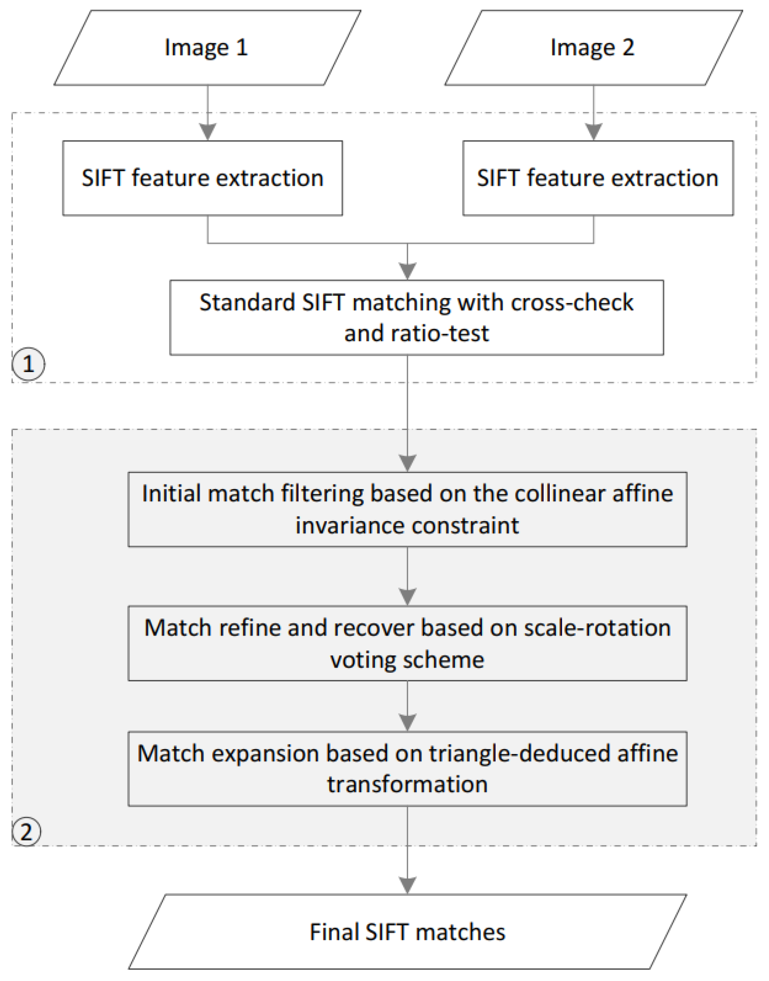
Combining the CAI and SOV constraints, this paper designs a reliable outlier-removal algorithm, termed CAISAO. The overall workflow is shown in Figure 1, which mainly consists of two major steps. In the first step, initial matches are obtained based on the classical workflow of local feature matching. For two images, SIFT features are detected individually, and initial matches are calculated by comparing two sets of feature descriptors. As reported in [10], the cross-check and ratio-test strategies are used to remove a large proportion of false matches from initial matches. In the second step, outliers are removed gradually by executing the CAI and SOV constraints. First, based on the CAI geometric constraint, obvious outliers are removed. In this study, the CAI geometric constraint has a more global observation of initial matches, and is designed to increase the inlier ratio of initial matches. Second, the SOV geometric constraint is applied to estimate the scale and rotation transformation parameters between these two input images based on the HT voting scheme, which is designed to remove retained false matches and recover lost true correspondences. Third, after the refinement based on the CAI and SOV constraints, match expansion is finally executed, which could further increase the number of true matches. The details of each step are presented in the following sections.
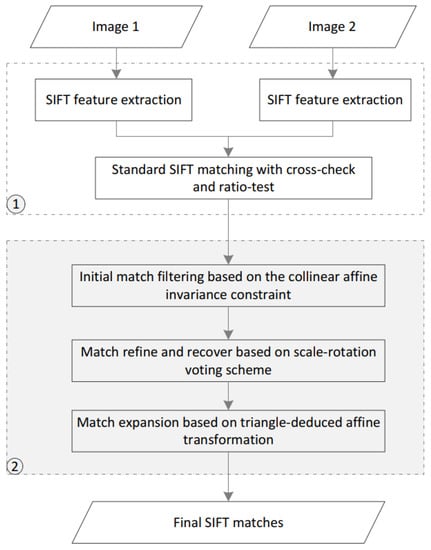
Figure 1.
The workflow of the proposed outlier-removal algorithm. Step 1 is initial matching; step 2 is outlier removal based on the proposed CAISOV.
2.2. Collinear Affine Invariance-Based Geometric Constraint
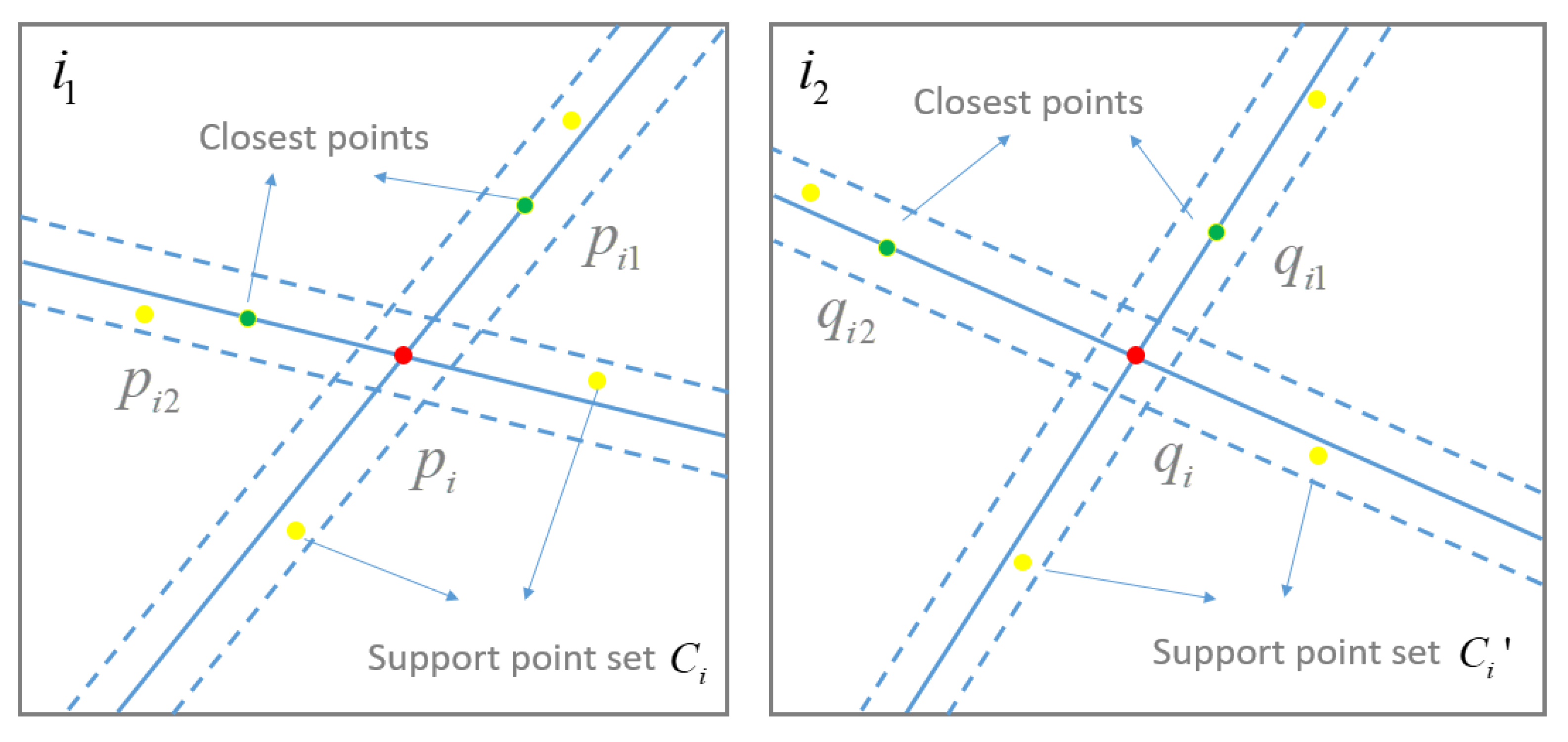
Initial matches are established by using the classical workflow of local feature matching. Considering the high computational costs in scale pyramid construction and feature descriptor comparison, the GPU (graphics processing unit) accelerated SIFT algorithm, termed SIFTGPU [35], has been utilized in this study to detect and match features. Due to geometric and photometric deformations, and the only usage of local appearances for descriptor generation, false matches have inevitably existed in initial matches. After the establishment of initial matches, false matches are then filtered based on the CAI geometric constraint. The basic idea of the CAI geometric constraint is that the collinearity of inliers is invariant under an affine transformation, which would be used to calculate the similarity score of initial matches, as illustrated in Figure 2.
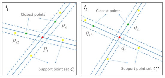
Figure 2.
The illustration of the CAI geometric constraint.
Suppose that feature points P and Q are detected from two input images and , respectively; n initial matches are obtained and indicated as with and . For each initial match , the similarity score is then calculated according to the CAI geometric constraint. For the target feature points in image , its K closest feature points are first searched from matched feature points of image . Then, a straight line is constructed by connecting the target feature point and one of its closest feature points . After the buffering operation on the straight line by using the buffer threshold , the search region around the straight line can be formed, and all matched feature points within the search region are labeled as the support point set between points and . Therefore, for the K closest feature points in , the union of the support point set is defined as the support point set of the target feature points . Similarly, the K closest feature points of the corresponding point in image can be directly determined according to the relationship of initial matches, and the support point set of the corresponding point can be found by using the same operation. Based on these two support point sets and , the similarity score of the initial match is defined by Equation (1)
where is the number of common feature points between support point sets and ; is the maximal number of elements of support point sets and , i.e., . The similarity score indicates the probability that one initial match belongs to the true correspondences, which are deduced from its supporting point set.
2.3. Scale-Orientation Voting-Based Geometric Constraint
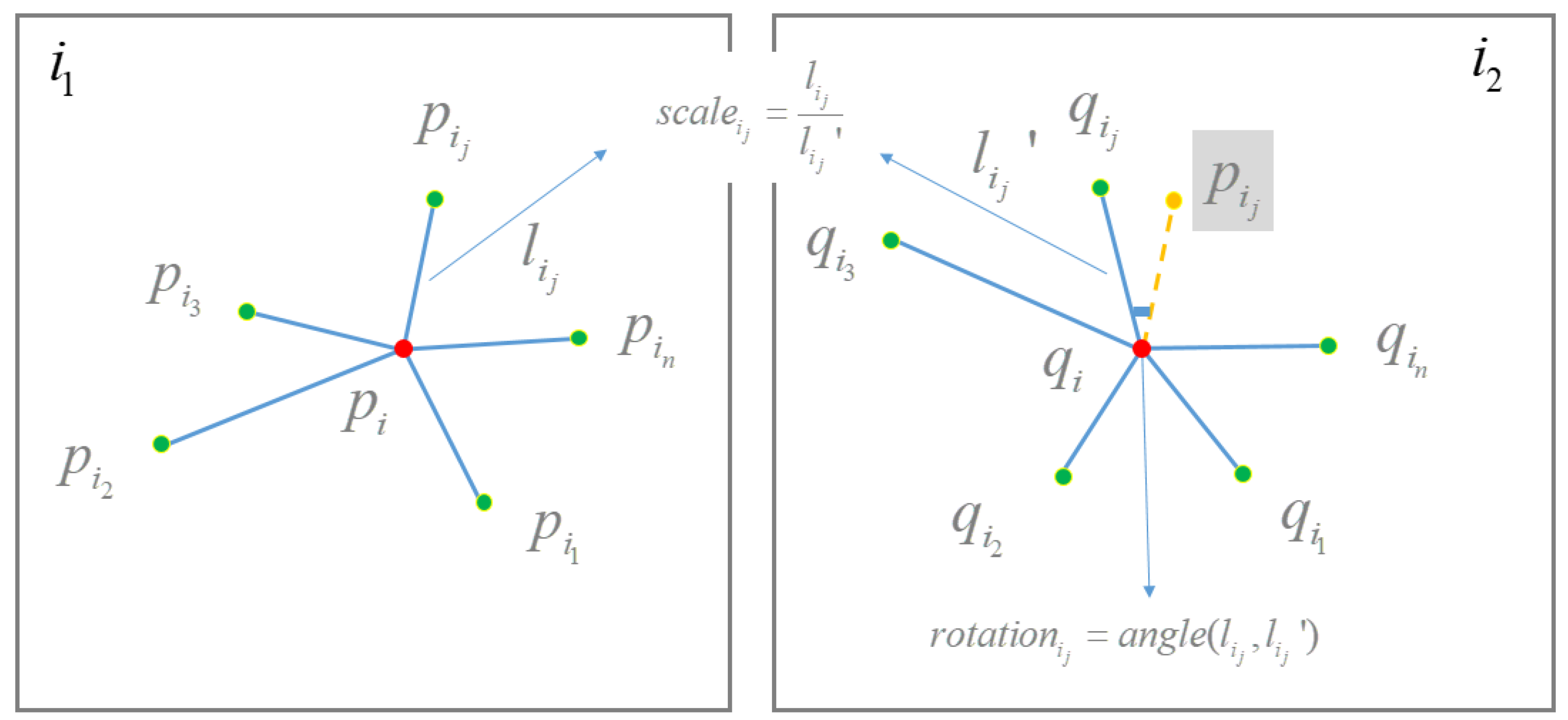
Obvious outliers can be removed based on the CAI geometric constraint. Due to relativly lower discriminative power, and the global construction of support point sets, false matches would still exist in the filtered matches, and a proportion of true matches would be removed at the same time. Therefore, inspired by the work of [25], this study further uses the scale-orientation voting to refine matches and retrieve falsely removed inliers, as illustrated in Figure 3.
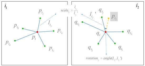
Figure 3.
The illustration of the SOV geometric constraint.
Suppose that the refined matches are generated based on the CAI geometric constraint; for one target match , its neighboring match can be found under the constraint that is the neighbor of , and is the neighbor of . Two lines and can then be created by connecting one target feature point with its neighboring feature points, i.e., connects and ; connects and . Thus, the scale change from feature point to is defined as the length ratio of lines and by Equation (2)
Similarly, the orientation change from feature point to is defined as the anticlockwise angle that rotates line to line , as represented by Equation (3)
Based on the definition of scale and orientation, the HT voting scheme is then used to find the correct scale and orientation range. The core idea is that the votes of inliers in scale and orientation are accumulated in the voting space; conversely, the votes of outliers are randomly distributed in the voting space. In this study, 9 ranges are used as the voting bins of scales, which are represented as ; 36 ranges are used as the voting bins of rotation, which are defined with an interval value of and range from to . Thus, the purpose of finding the correct scale and orientation range is cast as finding the bin with peak values in the voting space. For one target match , K nearest neighbors and of matched points and are first determined, and the lines and created by using the matched point and one of its nearest neighbors are used to calculate the scale and rotation based on Equations (2) and (3), and they are then used to vote bins of scale and rotation. After the voting of all matches in , the bins with peak votes define the correct scale and rotation changes from image to . In other words, matches are labeled as inliers if their scale and rotation are within the correct ranges.
2.4. Implementation of the Proposed Algorithm
Based on the CAI and SOV geometric constraints as presented in Section 2.2 and Section 2.3, this study implements a reliable outlier-removal algorithm. The workflow of the proposed algorithm consists of three major steps: (1) initial matches that are generated by using the classical local feature matching are refined based on the CAI geometric constraint, in which obvious outliers are eliminated to increase the inlier ratio; (2) by using the refined matches, the SOV constraint is then executed to find the correct scale and rotation parameters between image pairs, which are used to remove retained false matches and recover falsely removed true matches; (3) finally, match expansion is conducted by using the transformation that is deduced from two corresponding triangles. The details of the workflow are presented as follows:
- (1)
- Outlier removal based on the CAI geometric constraint. According to Equation (1), the similarity score of each match can be calculated. To cope with high outlier ratios, initial matches with the similarity score that equals zero are first directly eliminated. For the remaining matches, the similarity score is calculated again, and the matches with a similarity score less than a pre-defined threshold are removed. The above-mentioned operations are iteratively executed until the similarity scores of all matches are greater than . In this study, the threshold is set as 0.1.
- (2)
- Outlier removal based on the SOV geometric constraint. After the execution of step (1), the retained matches with higher inlier ratios are then used to search the correct scale and rotation parameters between image pairs and . The matches are labeled as inliers if their scale and rotation parameters fall into the correct voting bins; otherwise, the matches are labeled as outliers. To recover falsely removed matches, match expansion is simultaneously executed in this step. In detail, for each removed match , the scale and rotation parameters are calculated again. If these parameters fall into the correct voting bin, the match is grouped with the inliers.
- (3)
- Match expansion based on the triangle constraint. After the execution of CAI and SOV constraints, refined matches with high inlier ratios can be obtained. To further recover more inliers, match expansion is conducted again based on the transformation deduced from corresponding triangles, as presented in [29]. During match expansion, refined matches are used to construct the Delaunay triangulation and its corresponding graph. For each feature point , candidate feature points are found by using the transformation that is deduced from two corresponding triangles, and the classical local feature matching is executed between feature point and candidate feature points . The workflow of the proposed CAISOV algorithm is presented in Algorithm 1.
| Algorithm 1 CAISOV |
Input: Initial candidate matches M Output: final matches
|
3. Experimental Results
For performance evaluation, three close-range image datasets and two UAV remote-sensing image datasets have been used in the experiments. First, the influence of the distance threshold for support-point searching is analyzed by using a close-range benchmark dataset. Second, the robustness of the proposed algorithm to outliers is analyzed for varying outlier ratios. Third, the details of outlier removal are presented by using both rigid and non-rigid image pairs. Finally, the proposed algorithm is compared comprehensively with classical outlier-removal methods, and its application to UAV image orientation based on SfM (Structure from Motion) is also presented.
3.1. Datasets and Evaluation Metrics
Three close-range image datasets and two UAV remote-sensing datasets are utilized for the performance evaluation in this study. The three close-range image datasets include both rigid and non-rigid image pairs.
- The first dataset is the well-known benchmark dataset, termed the Oxford dataset, which has been widely used for the evaluation of feature detectors and descriptors [36], as presented in Figure 4. This dataset consists of a total number of eight image sequences, in which each image sequence has six images with varying photometric and geometric deformations, e.g., changes of viewpoint and illumination, motion blur, and scale and rotation.
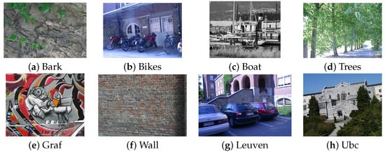 Figure 4. The Oxford dataset (close-range dataset 1).
 - The second dataset is the well-known HPatches benchmark [37], which has been widely used for training and testing feature descriptors based on CNN models. Similar to the Oxford dataset, 117 image sequences that consist of 6 images have been prepared in this dataset, among which 8 image sequences have been selected for the performance evaluation in rigid image matching, as shown in Figure 5.
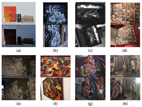 Figure 5. (a–h) The rigid dataset (close-range dataset 2).
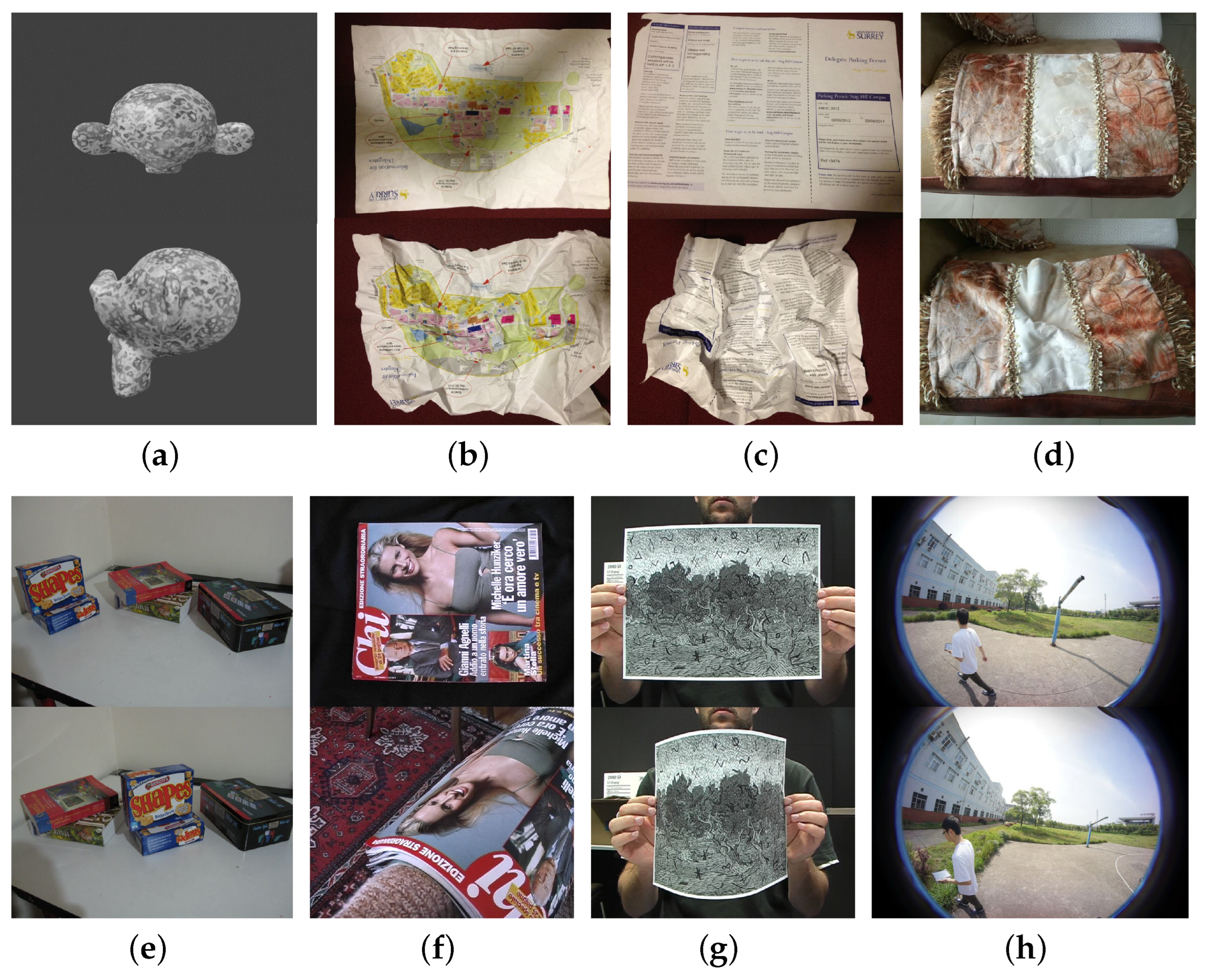
 - The third dataset includes 8 image pairs that have non-rigid deformations, such as blend and extrusion, as shown in Figure 6. For the used three datasets, the first and second datasets have the ground-truth transformation between image pairs, such as the homography matrix for the first and the other images in each image sequence. For these two datasets, the provided model parameters have been used to separate inliers from initial matches. In this study, the matches with the transformation errors that are less than 5 pixels are defined as inliers. For the third dataset, we have prepared ground-truth data through manual inspection.
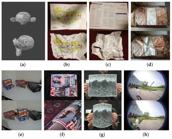 Figure 6. (a–h) The non-rigid dataset (close-range dataset 3).
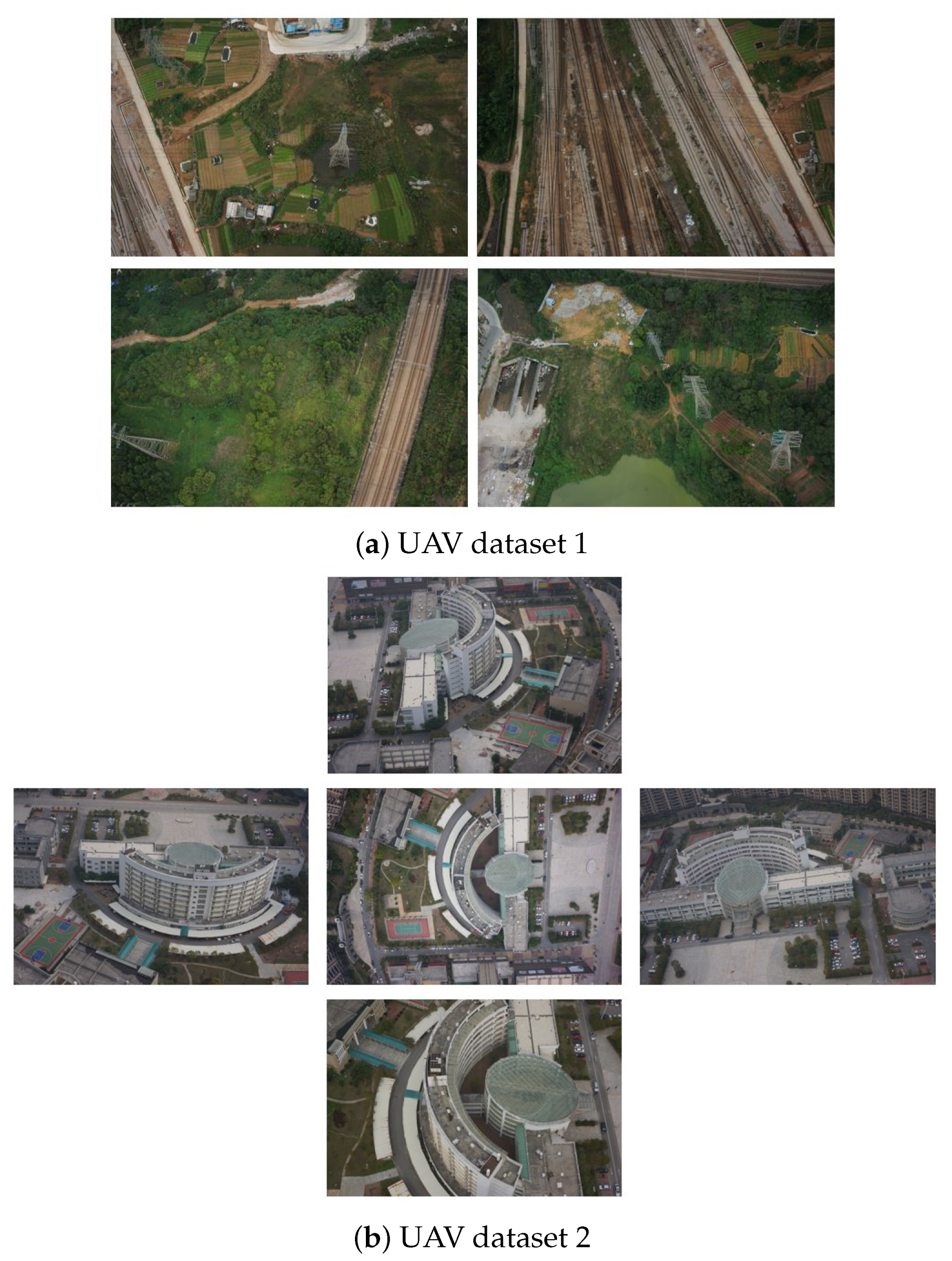
To verify the application of the proposed outlier-removal algorithm to remote-sensing images, two UAV datasets are also selected in this study. The first dataset is collected from a suburban region, which is mainly covered by vegetation with some crossed railways. By using a two-camera imaging system equipped with Sony RX1R cameras, a total number of 320 images have been recorded at a flight height of 165 m, whose resolution is 6000 by 4000 pixels. The second dataset is collected from one urban resident region that is centered on a shopping plaza and surrounded by high buildings. In this test site, a multi-rotor UAV platform equipped with one penta-view photogrammetric imaging system has been utilized for outdoor data acquisition, which can capture images from five directions and facilitate 3D modeling of urban buildings. At a flight height of 175 m, a total number of 750 images have been recorded with simensions of 6000 by 4000 pixels. Figure 7 illustrates the images of these two UAV datasets.

Figure 7.
The illustration of these two UAV datasets.
For comparative performance evaluation, three criteria, namely precision, recall and inlier number, are utilized as measurements. Precision is the ratio of the numbers of inliers and total matches generated from the proposed algorithm, as presented by Equation (4); recall is the ratio of the number of inliers to the number of total inliers in the ground-truth data, as shown by Equation (5); inlier number is the total number of true matches that are generated by outlier-removal methods.
3.2. The Influence of the Collinear Distance Threshold on Outlier Removal
In the proposed CAISOV outlier-removal algorithm, the collinear distance threshold determines the buffer region of one line that connects the target point and its neighbor point, which directly influences the searching of support points in the CAI geometric constraint. In this section, we analyze the influence of the distance threshold on outlier removal and select the optical value for the remaining analysis and comparison.
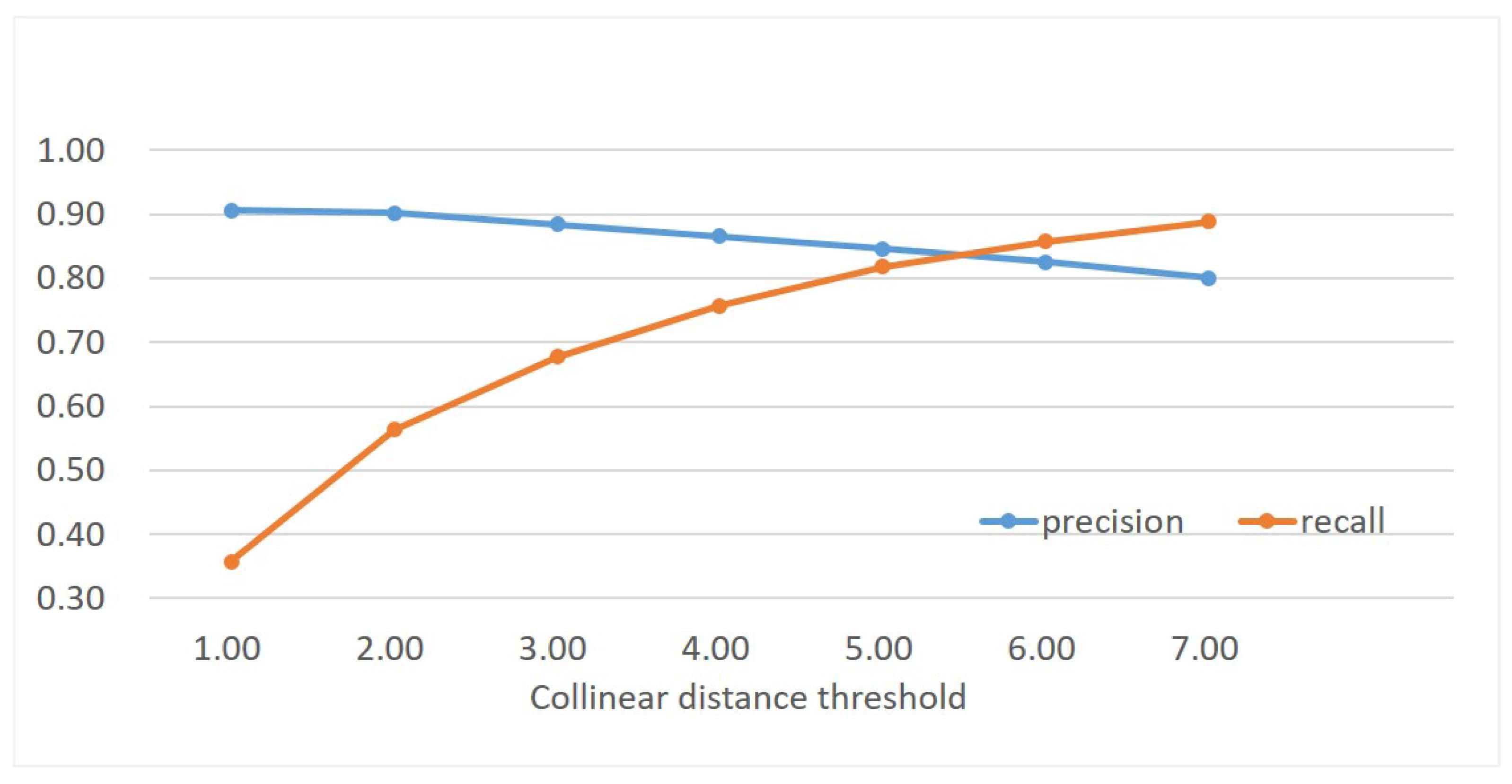
For performance evaluation, the first dataset (close-range dataset 1) has been used in this experiment. For each image sequence, five image pairs can be made by using the first image and one of the others, in which photometric and geometric deformations increase gradually. Thus, there are a total of 40 image pairs, and the average precision and recall have been calculated. Moreover, the collinear distance threshold is sampled from 1.0 to 7.0 with an interval value of 1.0. Figure 8 presents the statistical results. It is clearly shown that, with the increase of the collinear distance threshold, the metric recall increases. This is obviously because more and more support points can be found and further increase the value of the similarity score. The maximal value of recall reaches 0.9 when the collinear distance threshold is 7.0. Conversely, the metric precision gradually decreases with the increase of the collinear distance threshold. The main reason is that false matches are prone to be classified as inliers when the threshold is too large. To make a balance between precision and recall, the collinear distance threshold is set as 5.0 in the following tests.
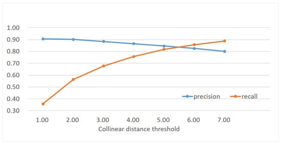
Figure 8.
The influence of the collinear distance threshold on image matching.
3.3. The Analysis of the Robustness to Outliers of the Algorithm
The robustness to varying outlier ratios is a very critical characteristic for outlier removal which influences the validation and performance of outlier-removal algorithms. In this section, we analyze the robustness to outliers for the proposed algorithm. Similar to Section 3.2, the first dataset (close-range dataset 1) has been used for this test. To prepare image pairs with specified outliers, inliers are first identified by using the ground-truth transformation, and a specified number of the remaining feature points are randomly added into the inliers to create matches with the specified outlier ratio. In this test, the outlier ratio ranges from 0.1 to 0.9 with an interval value of 0.1, and match expansion in the third step is not performed.
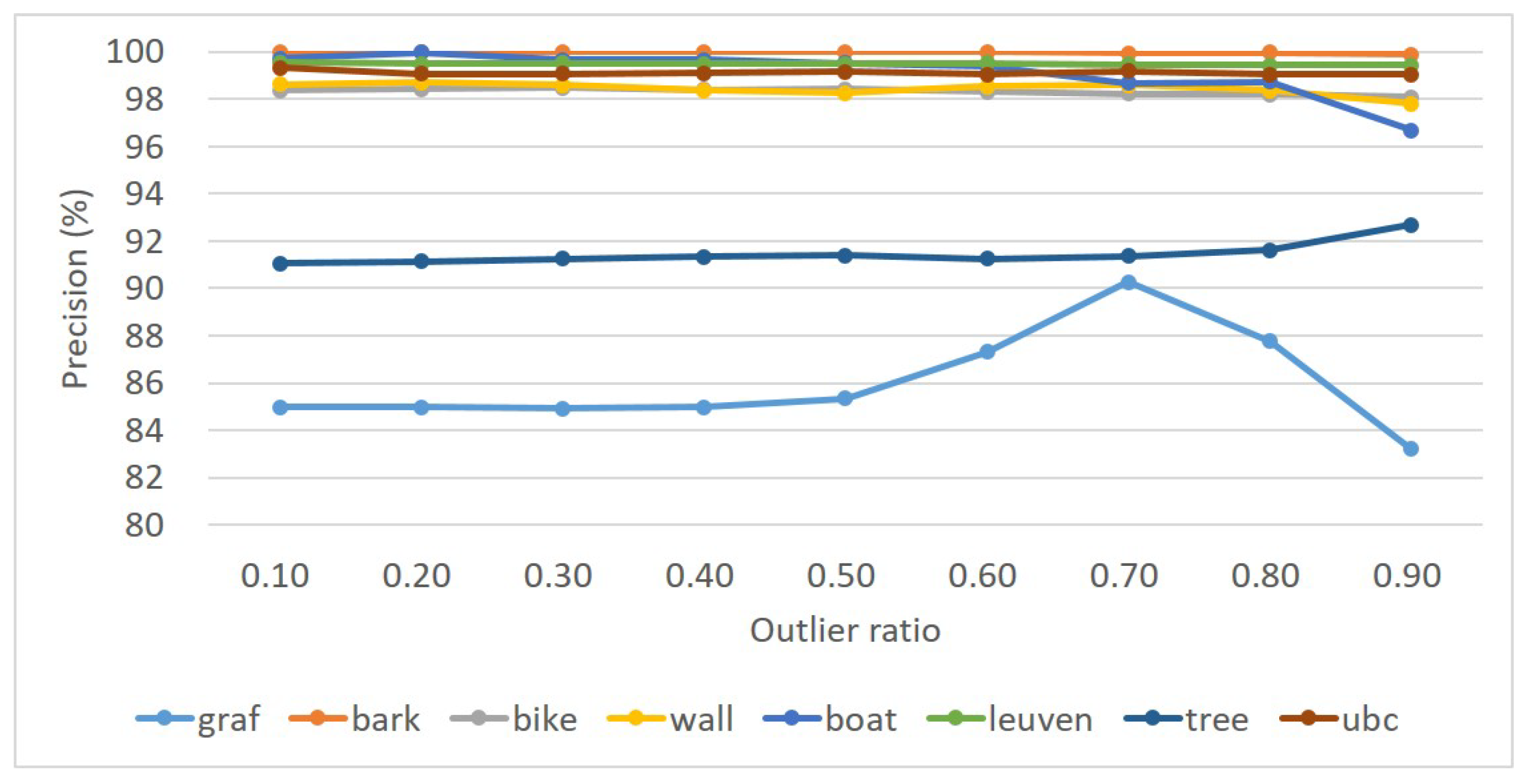
For performance evaluation, the average precision and recall of five image pairs are calculated for each image sequence. Figure 9 and Figure 10 present the statistical results of precision and recall, respectively. The experimental results show that the precision is almost constant with the increase of outlier ratios, and high precision has been achieved for the eight image pairs. Even when the outlier ratio reaches 0.9, the precision is still greater than , except for the image pairs graf and tree, as shown in Figure 9. By observation of the metric recall as shown in Figure 10, we find that a similar trend can also be observed with an increase of outlier ratios from 0.1 to 0.9. That is, the recall is almost constant for the eight image pairs, except for image pairs graf and tree. In addition, these image pairs can be divided into three groups. The first group includes image pairs bark, leuven and ubc, whose recall is approximately 0.95; the second group consists of image pairs bike, wall, boat and tree, whose recall ranges from 0.8 to 0.9. In conclusion, the proposed outlier-removal algorithm can achieve stable precision and recall under varying outlier ratios; the precision is very high even under the outlier ratio with the value of 0.9.
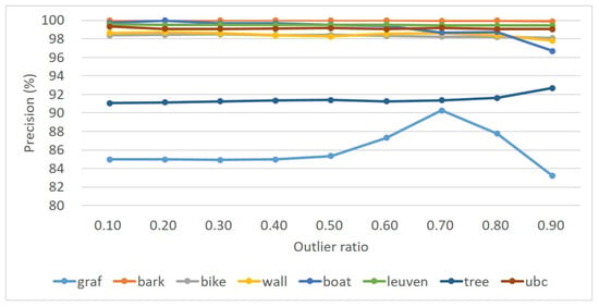
Figure 9.
Statistical results for the precision for the eight sequences in dataset 1.
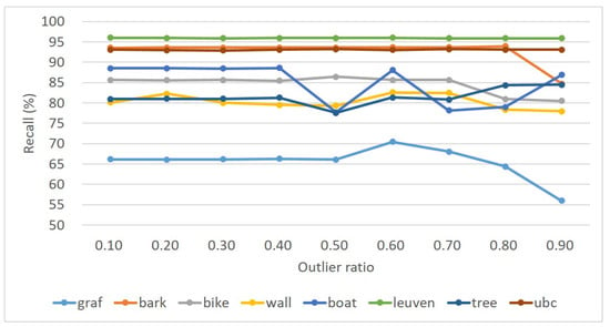
Figure 10.
Statistical results for the recall for the eight sequences in dataset 1.
3.4. Outlier Elimination Based on the Proposed Algorithm
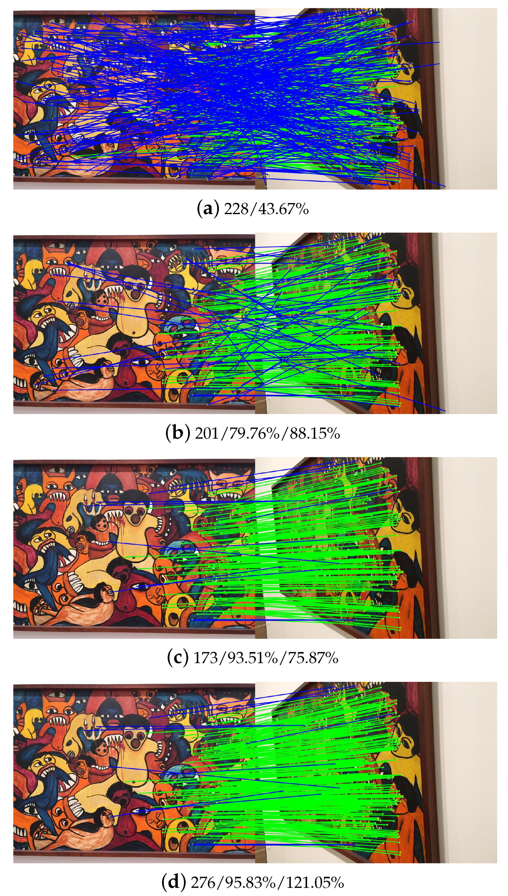
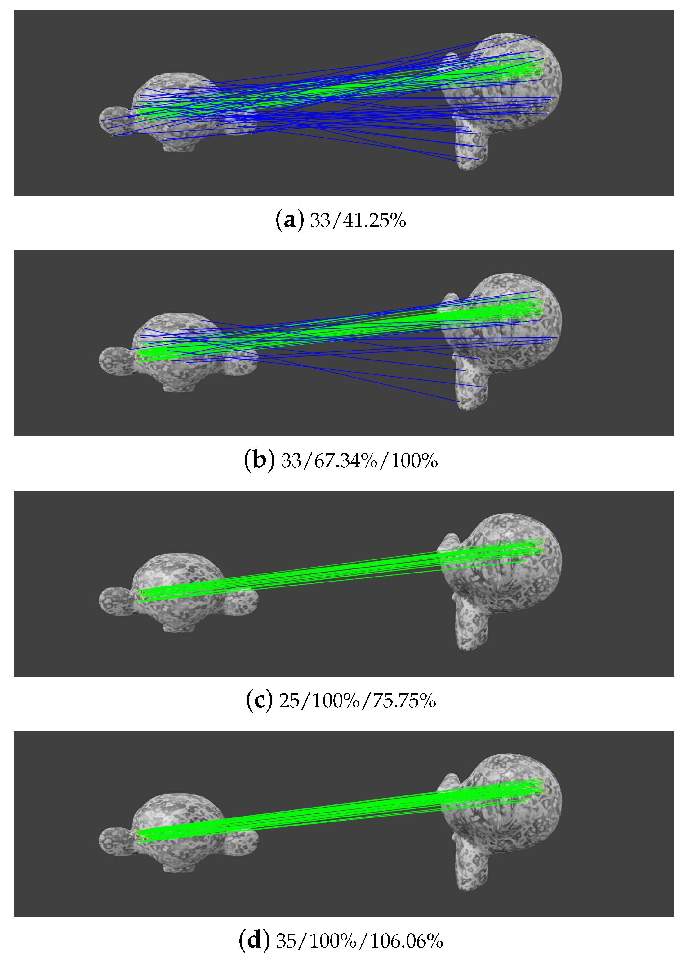
To obtain further insight from the analysis, two image pairs that come from the second rigid dataset (close-range dataset 2) and the third non-rigid dataset (close-range dataset 3) are selected to analyze the intermediate steps in the workflow of the proposed outlier-removal algorithm. Figure 11 and Figure 12 present the experimental results for the rigid and non-rigid image pairs, respectively. For each image pair, the results of four intermediate steps are collected and reported, which include initial match, collinear constraint, scale-orientation voting, and match expansion.
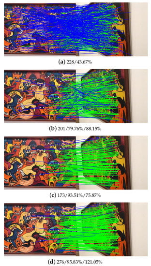
Figure 11.
Image matching of one rigid pair from dataset 2. The values in sub-title (a) indicate the number of initial matches and its precision; the values in other sub-titles indicate the number of refined matches and its precision and recall.
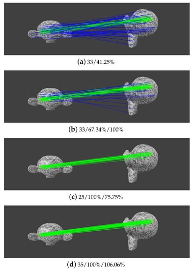
Figure 12.
Image matching of one rigid pair from dataset 3. The values in sub-title (a) indicate the number of initial matches and its precision; the values in other sub-titles indicate the number of refined matches and its precision and recall.
For the rigid case, as shown in Figure 11, the results of the four steps are presented in Figure 11a–d, respectively. For initial matches, there are 228 inliers with a precision of 43.67%. After the execution of the CAI constraint, 201 inliers are retained with a recall of 88.15%, and the precision increases to 79.76%. As shown in Figure 11b, a large proportion of outliers have been removed, which are rendered in blue lines. SOV is then conducted to further refine the matches, and the precision increases to 93.51%. In this step, 173 inliers are retained with a recall of 75.87%. Although some inliers are lost in the collinear constraint and the scale-orientation voting, match expansion is executed to resume falsely removed inliers at last. In this case, a total number of 276 inliers are retained with a precision value of 95.83%, as shown in Figure 11d.
For the non-rigid image pair as shown in Figure 12, there are 33 inliers in initial matches with a precision of 41.25%. After the execution of the CAI constraint, all inliers are retained and the precision increases to 67.34%, as shown in Figure 12b. We can see that some false matches still exist. SOV is then conducted, which eliminates the remaining outliers and increases the precision to 100% with a sacrifice of recall of 75.75%. Finally, match expansion retrieves falsely removed inliers, which generates 35 inliers with a precision of 100%, as shown in Figure 12d. Based on the observation of the intermediate results, we find that: (1) the collinear constraint can cope with high outlier ratios and increase the precision of initial matches; (2) although high precision can be obtained from scale-orientation voting, the recall of this geometric constraint is relatively low, which can be enhanced by match expansion. In a word, the proposed outlier-removal algorithm achieves high precision and recall for both rigid and non-rigid image pairs.
3.5. Comparison with State-of-the-Art Methods
In this section, the proposed algorithm is compared with the other methods, including RANSAC, K-VLD (K Virtual Line Descriptor), WGTM (Weighted GTM), LLT (Locally Linear Transforming), GMS (Grid-based Motion Statistic), and LAM (Locality Affine Invariant). K-VLD adopts the virtual line descriptor as the local photometric constraint to detect false matches [38]; WGTM is the classical outlier-removal method based on graph matching [32]; LLT is based on the local geometric constraint that is invariant between rigid and non-rigid image pairs [33]; GMS uses the motion smoothness constraint to translate feature number to match quality [34]; LAM depends on the local barycentric coordinate (LBC) and matching coordinate matrices (MCMs) for outlier removal [39]. In this comparison, the outlier ratio of initial matches is greater than 60%.
3.5.1. Performance Comparison Using the Rigid Dataset
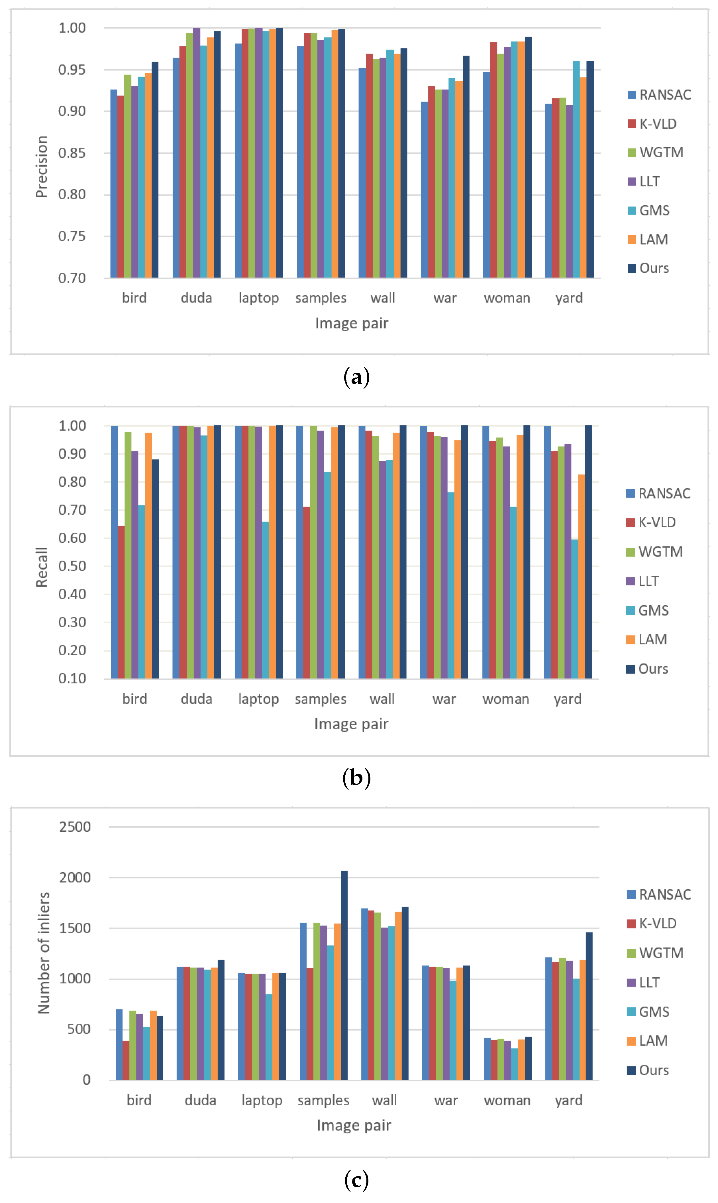
The performance of the selected methods is first evaluated by using the rigid dataset (close-range dataset 2), as shown in Figure 5. In this test, four metrics, namely precision, recall, inlier number and time, are used to evaluate the performance of the selected methods. Table 1 lists the statistical results of all image pairs, in which the values in the brackets indicate the statistical results without match expansion. The results listed in Table 1 are the average value of each metric. In addition, Figure 13 shows the statistical results in terms of precision, recall and inlier number. It is shown that the proposed algorithm achieves the highest precision among all compared methods, which reaches 97.27% and 98.06% without and with match expansion, respectively. LAM ranks second with a value of 97.02%. When considering the metric recall, RANSAC achieves the best performance with a value of 99.99%, which is followed by WGTM with a value of 97.36%. For the proposed algorithm, the scale-rotation voting strategy decreases the recall although high precision can be achieved, which has been demonstrated in Section 3.4. With the usage of match expansion, lost inliers can be recovered and the number of inliers is 1210 for the proposed algorithm. In this test, the average time cost of the proposed algorithm is 1.054 s, which ranks fifth among all methods. The main reason is that the number of initial matches is very large, which causes high computation costs in the CAI constraint.

Table 1.
Statistical results for the rigid dataset (value in the bracket indicates the statistical results without match expansion).
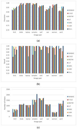
Figure 13.
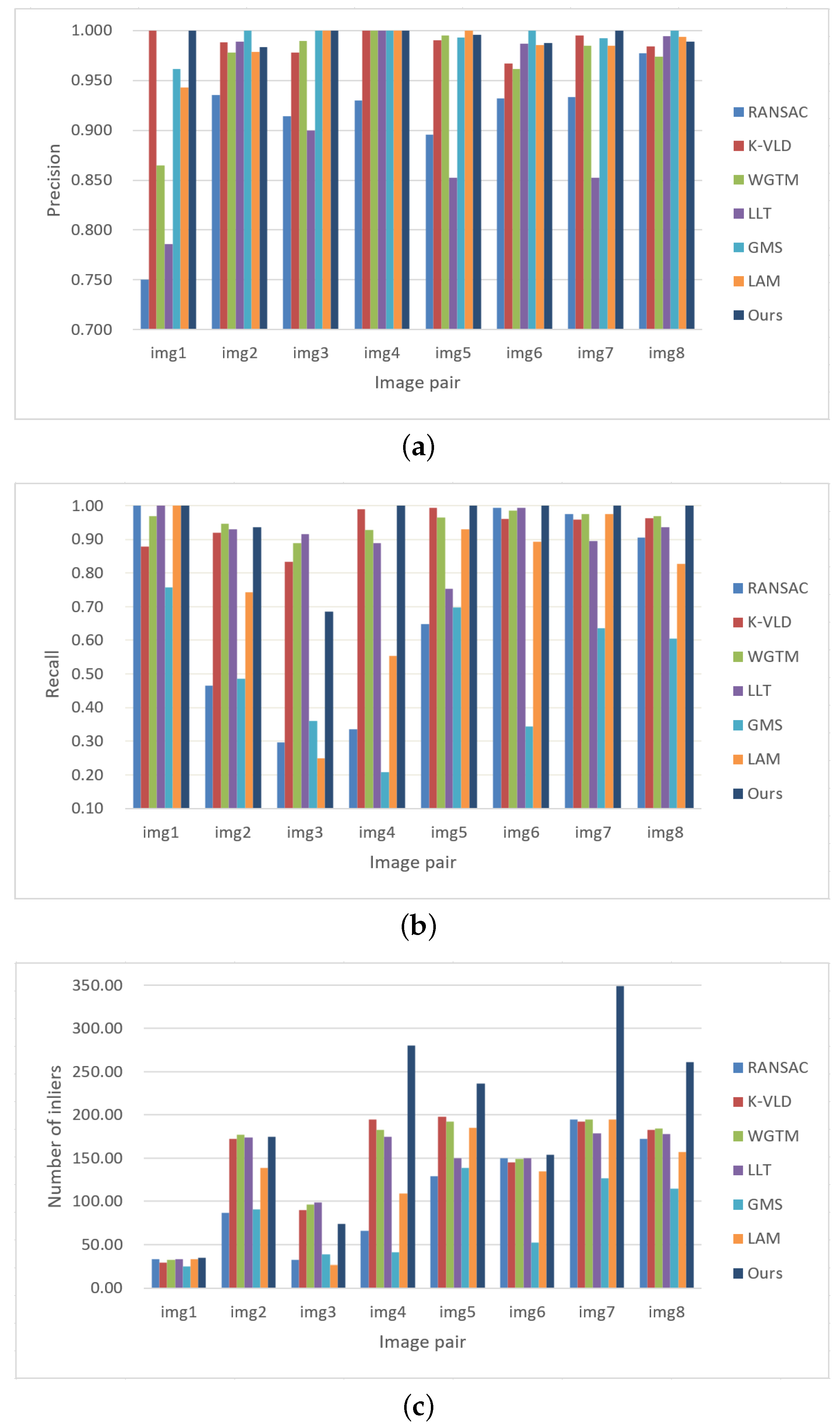
Statistical results for the rigid dataset (dataset 2): (a) precision; (b) recall; (c) number of inliers.
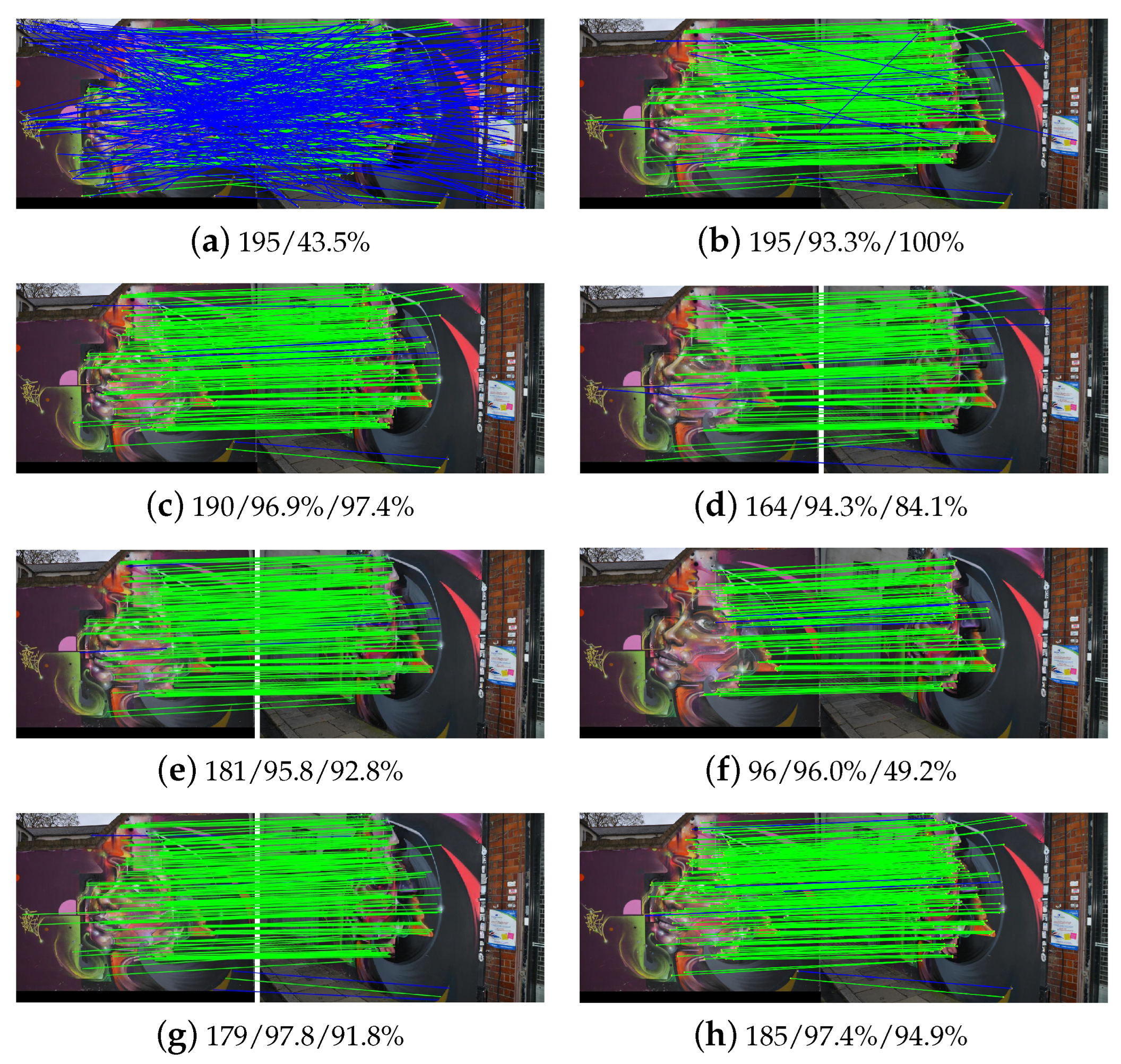
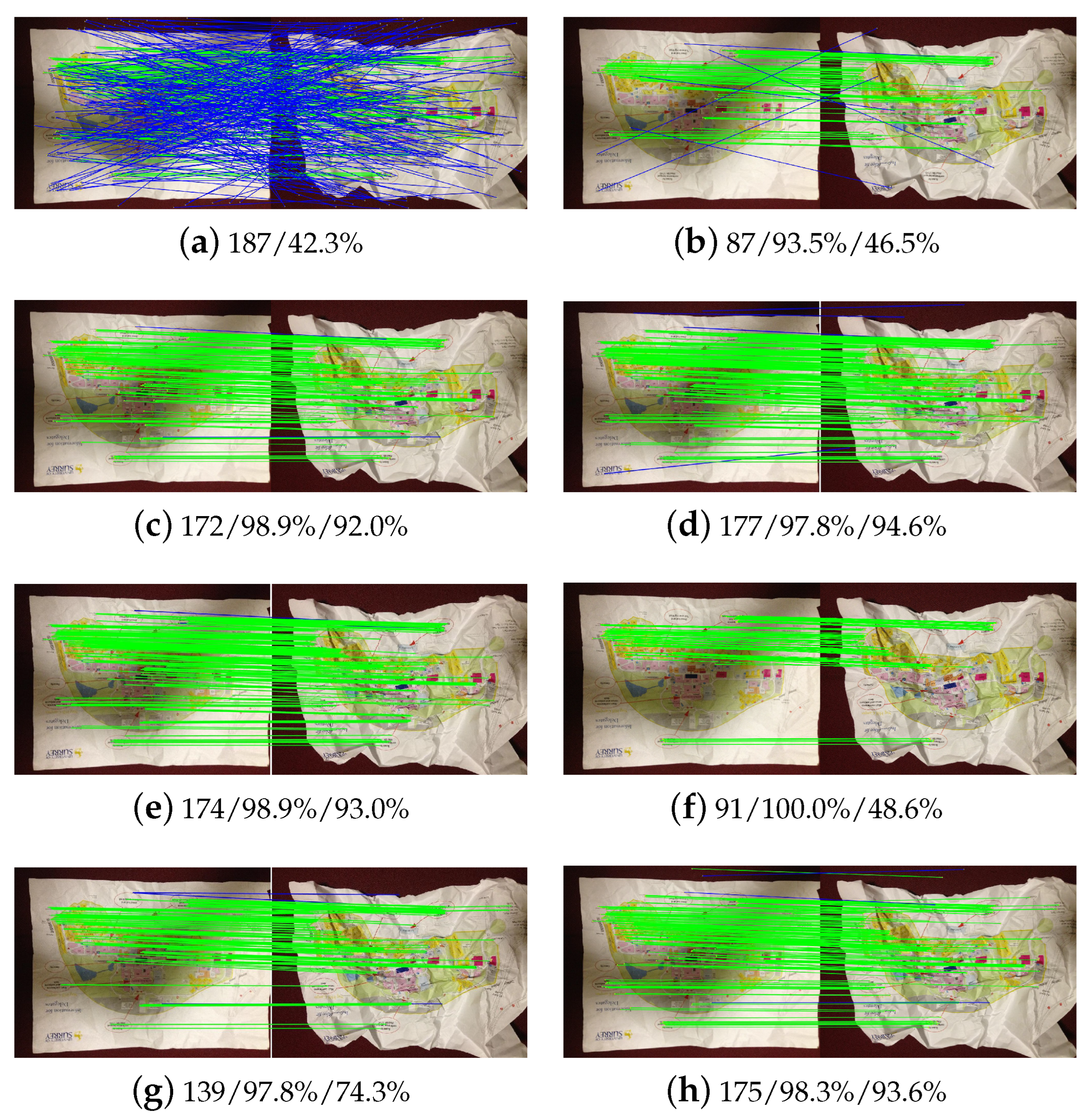
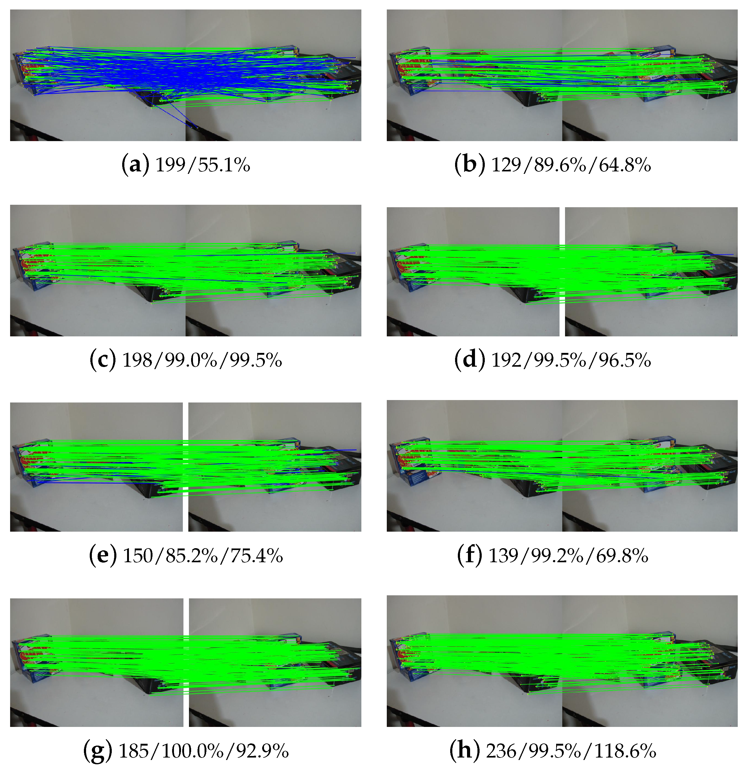
For further comparison, Figure 14, Figure 15 and Figure 16 illustrate the results of three image pairs in the rigid dataset, in which large changes in scale and viewpoints exist. For these three figures, the values in sub-title (a) indicate the number of initial matches and its precision; the values in other sub-titles indicate the number of refined matches and its precision and recall. For all the three image pairs, we can see that the proposed algorithm achieves the highest precision in Figure 14, the second-highest precision in Figure 15 and Figure 16, which is 92.3%, 97.4%, and 93.6% for the three image pairs, respectively. The GMS algorithm achieves the highest precision in Figure 16, but it retains only three matches. K-VLD and LLT have a high recall for the three image pairs. However, their precision is lower than the proposed algorithm, especially for image pairs 6 and 8 as shown in Figure 14 and Figure 16, respectively. For GMS, its recall is obviously lower than precision for the three image pairs. In addition, RANSAC achieves a very high recall for the three datasets since it is suitable for rigid image pairs.
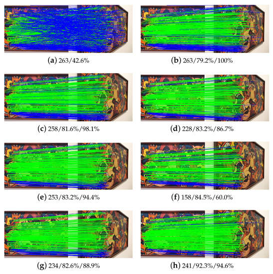
Figure 14.
Matching results of image pair 6 in the rigid dataset: (a) initial matches; (b) RANSAC; (c) K-VLD; (d) WGTM; (e) LLT; (f) GMS; (g) LAM; (h) Ours.
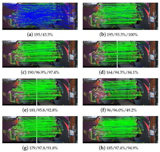
Figure 15.
Matching results of image pair 7 in the rigid dataset: (a) initial matches; (b) RANSAC; (c) K-VLD; (d) WGTM; (e) LLT; (f) GMS; (g) LAM; (h) Ours.
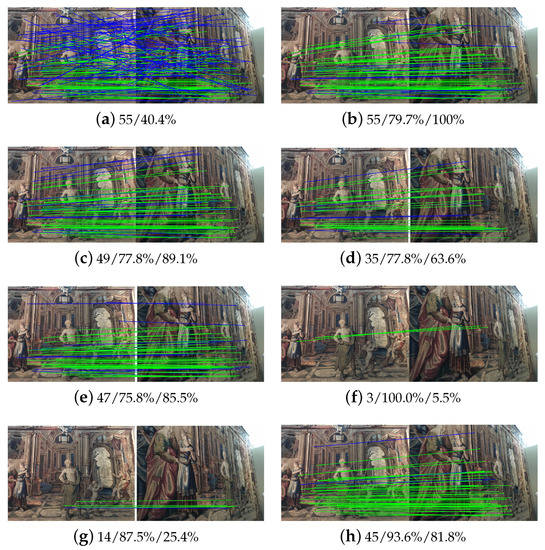
Figure 16.
Matching results of image pair 8 in the rigid dataset: (a) initial matches; (b) RANSAC; (c) K-VLD; (d) WGTM; (e) LLT; (f) GMS; (g) LAM; (h) Ours.
3.5.2. Performance Comparison Using the Non-Rigid Dataset
The performance of selected methods is first evaluated by using the non-rigid dataset (close-range dataset 3), as shown in Figure 6. Similar to Section 3.5.1, four metrics are used for performance evaluation. Table 2 and Figure 17 show the statistical results of the eight image pairs. We can see that for the non-rigid dataset, GMS achieves the highest precision with a value of 99.23%, which is followed by the proposed algorithm with a value of 99.19% for the test without match expansion; K-VLD ranks third with a precision of 98.77%. Due to its dependency on a pre-defined transformation model, RANSAC has the lowest precision in the non-rigid dataset. Similar to the performance in the rigid dataset, the recall of the proposed algorithm is relative lower than K-VLD, WGTM, LLT and LAM when match expansion is not executed. On the contrary, the number of inliers increases dramatically after match expansion. In contrast to the time cost in the rigid dataset, the efficiency of the proposed algorithm ranks second among all compared methods.

Table 2.
Statistical results for the non-rigid dataset (value in the bracket indicates the statistical results without match expansion).
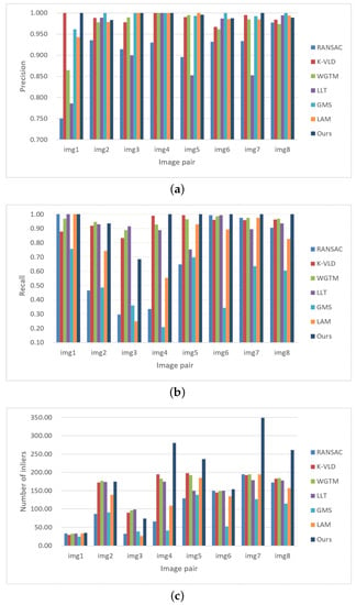
Figure 17.
Statistical results for the non-rigid dataset (dataset 3): (a) precision; (b) recall; (c) number of inliers.
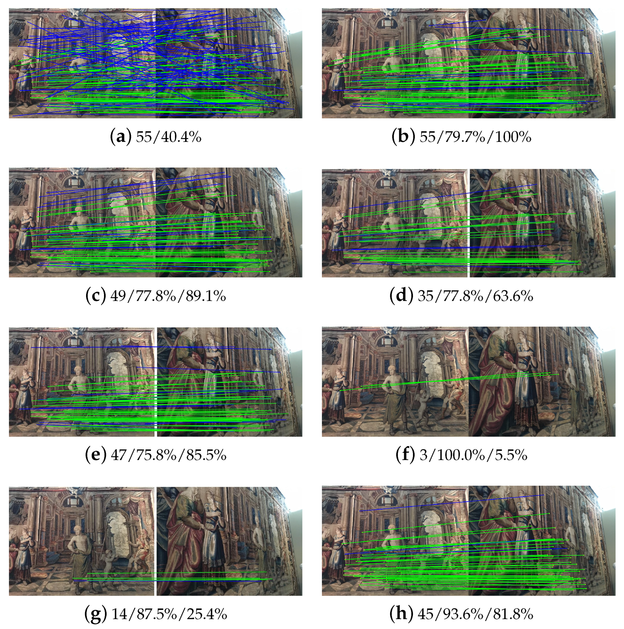
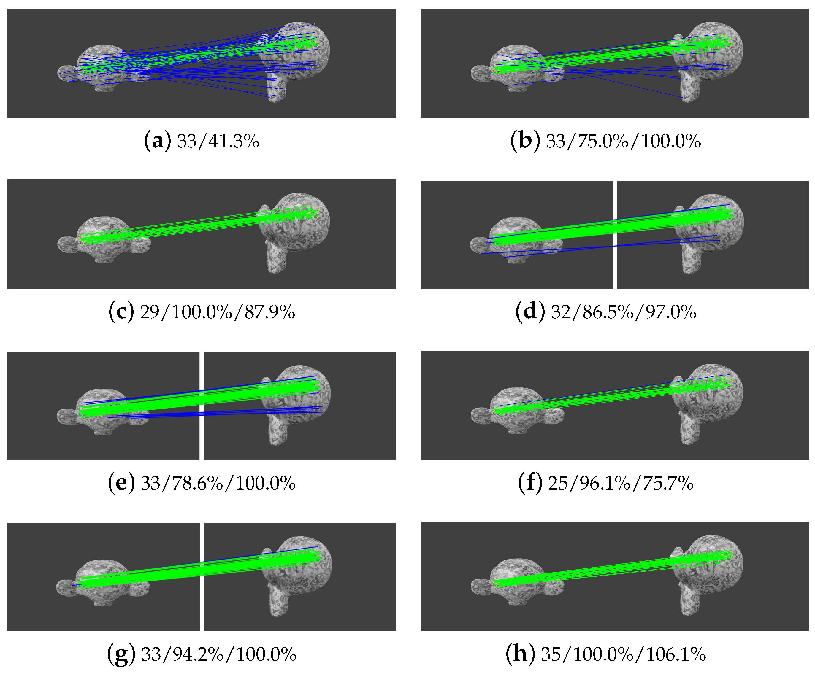
For further analysis, Figure 18, Figure 19 and Figure 20 illustrate the outlier-removal results of three image pairs in the non-rigid dataset. It is shown that the proposed algorithm achieves the best performance when considering these metrics. For image pair 1, as shown in Figure 18, the precision of WGTM and LLT are relatively lower than the proposed algorithm although they achieve high recall. Especially for LLT, its precision is 78.6% due to many false matches not being removed, as shown in Figure 18e. For image pair 2, as shown in Figure 19, all compared methods have good performance except for RANSAC as it relies on the specified model to separate outliers and cannot be adapted to non-rigid images. For image pair, 5 with multiple transformation models, K-VLD, WGTM, LAM and the proposed methods have good performance. Conversely, both precision and recall are low for LLT. Briefly, the proposed algorithm achieves the best overall performance for the three image pairs.
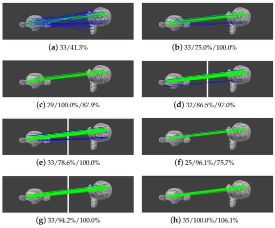
Figure 18.
Matching results of image pair 1 in the non-rigid dataset: (a) initial matches; (b) RANSAC; (c) K-VLD; (d) WGTM; (e) LLT; (f) GMS; (g) LAM; (h) Ours.

Figure 19.
Matching results of image pair 2 in the non-rigid dataset: (a) initial matches; (b) RANSAC; (c) K-VLD; (d) WGTM; (e) LLT; (f) GMS; (g) LAM; (h) Ours.
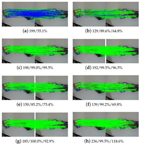
Figure 20.
Matching results of image pair 5 in the non-rigid dataset: (a) initial matches; (b) RANSAC; (c) K-VLD; (d) WGTM; (e) LLT; (f) GMS; (g) LAM; (h) Ours.
3.6. Application of the Proposed Algorithm for SfM-Based UAV Image Orientation
In this section, two UAV datasets have been used to verify the application of the proposed algorithm for remote sensing images. The proposed outlier-removal algorithm is embedded into a classical SfM-based image-orientation pipeline [40], which takes as input UAV images and produces camera poses and scene 3D points. In the SfM-based image orientation pipeline, overlapped image pairs are selected by using the vocabulary-based image-retrieval technique [2] after the execution of SIFT feature extraction. Guided by the selected image pairs, feature matching is then conducted by searching the nearest neighbor between their two descriptor sets. False matches are removed by using the proposed algorithm, which is finally fed into the SfM pipeline for image orientation.
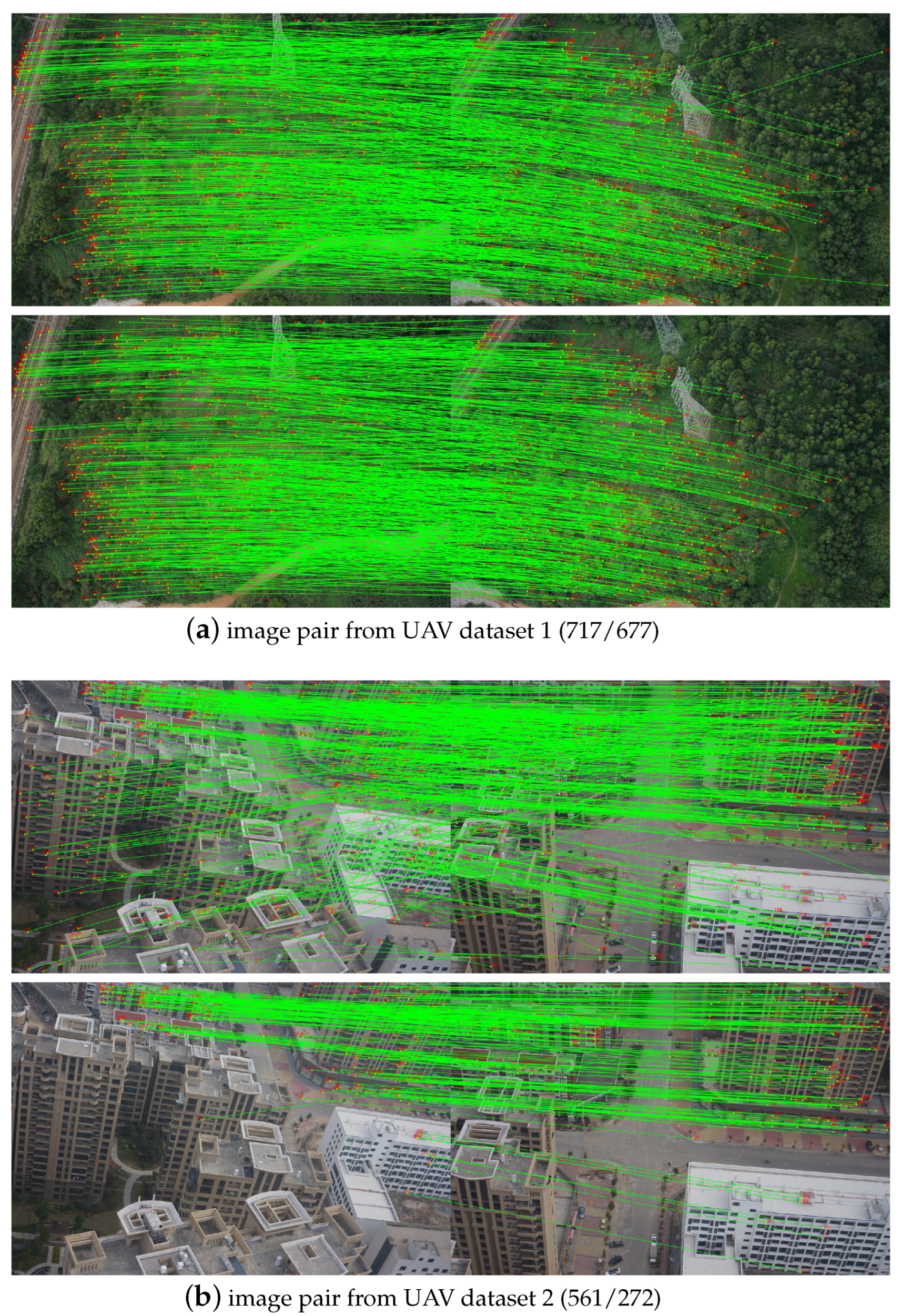
In this test, a total number of 1786 and 16,394 image pairs have been obtained for these two UAV datasets, respectively. Classical feature extraction and matching are then executed to search for initial candidate matches. Due to the limited discriminative power of local descriptors and the existence of repetitive patterns, many false matches can be found in the initial matches, as illustrated by the top sub-figures in Figure 21, in which two image pairs are selected from these two UAV datasets, respectively. Due to serious occlusions and repetitive patterns, many more false matches are observed from the second image pair. By using the proposed algorithm, false matches can be detected and removed, as demonstrated by the bottom sub-figures in Figure 21. Noticeably, RANSAC has not cooperated with the proposed algorithm in this test.
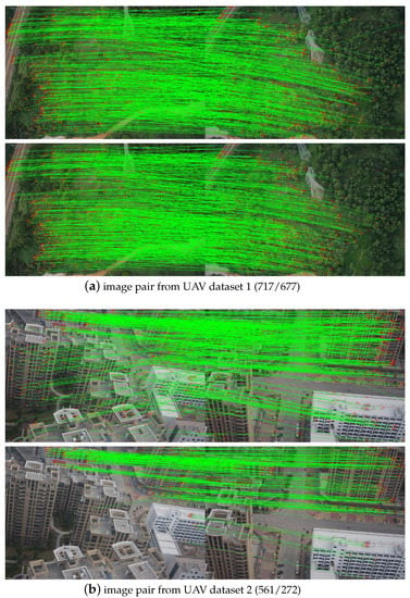
Figure 21.
The illustration of feature matching of image pairs from UAV datasets. The values in the bracket indicate the number of matches before and after outlier removal.
After outlier removal of all image pairs, refined matches can be obtained and fed into the SfM pipeline to achieve UAV image orientation. To evaluate the performance of the proposed algorithm, the matching results of RANSAC have also been used in this test. Table 3 lists the statistical results of SfM-based image orientation for the two UAV datasets. Three metrics, namely, efficiency, precision and completeness, are used for performance evaluation. The metric efficiency indicates time costs consumed in image orientation; the metric precision is the re-projection error in bundle adjustment optimization; the metric completeness is quantified by the numbers of resumed 3D points and connected images.

Table 3.
The statistical results of SfM-based image orientation for the two UAV datasets in terms of efficiency, completeness, and precision. The values in the bracket indicate the number of connected images in the final models.
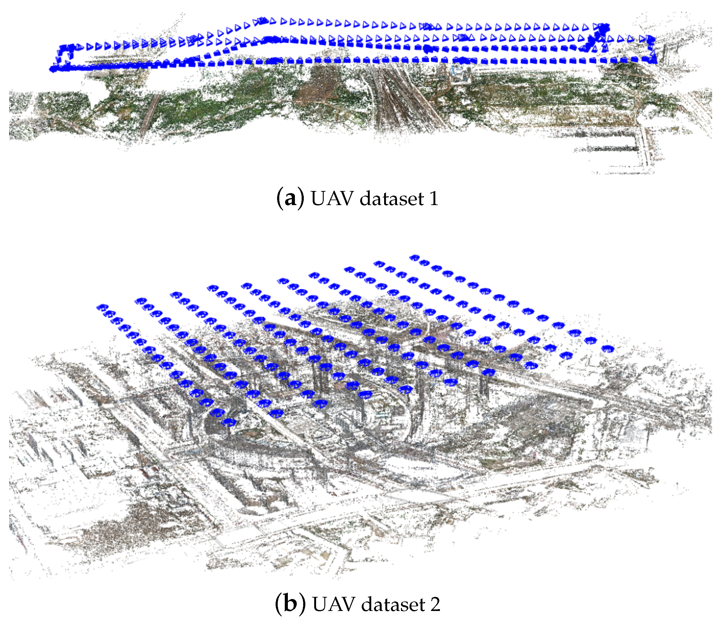
It is shown that for these two UAV datasets, both RANSAC and the proposed algorithm can provide enough reliable matching results for SfM-based image orientation since all images have been connected in this test. When considering the metrics’ efficiency, we can find that little more time cost is incurred by the proposed algorithm. The main reason is that the proposed algorithm provides more feature matches for SfM-based image orientation. This can be observed from the numbers of reconstructed 3D points, which are 236,800 and 379,989 for the proposed algorithm. For the two algorithms, comparative accuracy has been achieved. That is, the proposed algorithm can be used for outlier removal in both rigid and non-rigid images, and it can also provide reliable feature matches for UAV datasets. The SfM-based image orientation results by using the matches from the proposed algorithm are shown in Figure 22.

Figure 22.
The SfM-based image orientation by using the matching results from the proposed algorithm. Blue rectangles represent the oriented camera frames, and 3D points are rendered by using true image color.
4. Conclusions
In this study, we propose a reliable outlier-removal algorithm by combining two affine-invariant geometric constraints, termed CAI (collinear affine invariance) and SOV (scale-orientation voting) constraints. These two geometric constraints are hierarchically executed to remove outliers, and match expansion is finally performance to resume falsely removed inliers. The CAI geometric constraint is based on the observation that the collinear property of any two points is invariant to affine transformation. Compared with other local geometric constraints, it has two advantages. On one hand, its mathematical model is very simple; on the other hand, it has a more global observation of initial matches. The SOV geometric constraint is designed to remove remaining outliers and recover the lost inliers, in which the peaks of both scale and orientation voting define the parameters of the geometric transformation model. By using both close-range datasets (rigid and non-rigid images) and UAV datasets for experiments, the results demonstrate that the proposed algorithm can achieve the best overall performance compared with RANSAC-like and local geometric constraint-based methods, and it can also provide reliable feature matches for UAV datasets in SfM-based image orientation.
Author Contributions
Conceptualization, H.L.; Data curation, K.L.; Formal analysis, H.L.; Funding acquisition, S.J., Q.L. and L.W.; Investigation, K.L.; Project administration, L.W.; Resources, K.L., Q.L. and W.J.; Software, W.J.; Supervision, S.J.; Writing original draft, H.L. and S.J. All authors have read and agreed to the published version of the manuscript.
Funding
This research was financially supported by the National Natural Science Foundation of China (42001413), the Open Research Fund from Guangdong Laboratory of Artificial Intelligence and Digital Economy (SZ) (GML-KF-22-08), the Open Research Project of The Hubei Key Laboratory of Intelligent Geo-Information Processing (KLIGIP-2021B11), the Open Research Fund of State Key Laboratory of Information Engineering in Surveying, Mapping and Remote Sensing, Wuhan University (20E03), the Opening Fund of Key Laboratory of Geological Survey and Evaluation of Ministry of Education (GLAB2020ZR19) and the Fundamental Research Funds for the Central Universities, China University of Geosciences (Wuhan) (CUG2106314).
Acknowledgments
The authors would like to thank the anonymous reviewers and editors, whose comments and advice improved the quality of the work.
Conflicts of Interest
The authors declare no conflict of interest.
References
- Habib, A.; Han, Y.; Xiong, W.; He, F.; Zhang, Z.; Crawford, M. Automated Ortho-Rectification of UAV-Based Hyperspectral Data over an Agricultural Field Using Frame RGB Imagery. Remote Sens. 2016, 8, 796. [Google Scholar] [CrossRef]
- Jiang, S.; Jiang, W.; Guo, B. Leveraging vocabulary tree for simultaneous match pair selection and guided feature matching of UAV images. ISPRS J. Photogramm. Remote Sens. 2022, 187, 273–293. [Google Scholar] [CrossRef]
- Ye, Y.; Shan, J. A local descriptor based registration method for multispectral remote sensing images with non-linear intensity differences. ISPRS J. Photogramm. Remote Sens. 2014, 90, 83–95. [Google Scholar] [CrossRef]
- Sattler, T.; Leibe, B.; Kobbelt, L. Efficient & effective prioritized matching for large-scale image-based localization. IEEE Trans. Pattern Anal. Mach. Intell. 2016, 39, 1744–1756. [Google Scholar]
- Jian, M.; Wang, J.; Yu, H.; Wang, G.; Meng, X.; Yang, L.; Dong, J.; Yin, Y. Visual saliency detection by integrating spatial position prior of object with background cues. Expert Syst. Appl. 2021, 168, 114219. [Google Scholar] [CrossRef]
- Jiang, S.; Jiang, C.; Jiang, W. Efficient structure from motion for large-scale UAV images: A review and a comparison of SfM tools. ISPRS J. Photogramm. Remote Sens. 2020, 167, 230–251. [Google Scholar] [CrossRef]
- Fan, B.; Kong, Q.; Wang, X.; Wang, Z.; Xiang, S.; Pan, C.; Fua, P. A performance evaluation of local features for image-based 3D reconstruction. IEEE Trans. Image Process. 2019, 28, 4774–4789. [Google Scholar] [CrossRef]
- Jiang, S.; Jiang, W.; Guo, B.; Li, L.; Wang, L. Learned Local Features for Structure From Motion of UAV Images: A Comparative Evaluation. IEEE JOurnal Sel. Top. Appl. Earth Obs. Remote Sens. 2021, 14, 10583–10597. [Google Scholar] [CrossRef]
- Harris, C.; Stephens, M. A combined corner and edge detector. In Proceedings of the Alvey Vision Conference, Manchester, UK, 31 August–2 September 1988; Volume 15, pp. 147–151. [Google Scholar]
- Lowe, D.G. Distinctive image features from scale-invariant keypoints. Int. J. Comput. Vis. 2004, 60, 91–110. [Google Scholar] [CrossRef]
- Dong, J.; Soatto, S. Domain-size pooling in local descriptors: DSP-SIFT. In Proceedings of the IEEE Conference on Computer Vision and Pattern Recognition, Boston, MA, USA, 7–12 June 2015; pp. 5097–5106. [Google Scholar]
- Morel, J.M.; Yu, G. ASIFT: A new framework for fully affine invariant image comparison. SIAM J. Imaging Sci. 2009, 2, 438–469. [Google Scholar] [CrossRef]
- Sun, Y.; Zhao, L.; Huang, S.; Yan, L.; Dissanayake, G. L2-SIFT: SIFT feature extraction and matching for large images in large-scale aerial photogrammetry. ISPRS J. Photogramm. Remote Sens. 2014, 91, 1–16. [Google Scholar] [CrossRef]
- Han, X.; Leung, T.; Jia, Y.; Sukthankar, R.; Berg, A.C. Matchnet: Unifying feature and metric learning for patch-based matching. In Proceedings of the IEEE Conference on Computer Vision and Pattern Recognition, Boston, MA, USA, 7–12 June 2015; pp. 3279–3286. [Google Scholar]
- Simo-Serra, E.; Trulls, E.; Ferraz, L.; Kokkinos, I.; Fua, P.; Moreno-Noguer, F. Discriminative learning of deep convolutional feature point descriptors. In Proceedings of the IEEE International Conference on Computer Vision, Santiago, Chile, 7–13 December 2015; pp. 118–126. [Google Scholar]
- Mishchuk, A.; Mishkin, D.; Radenovic, F.; Matas, J. Working hard to know your neighbor’s margins: Local descriptor learning loss. In Proceedings of the 31st International Conference on Neural Information Processing Systems NIPS’17, Long Beach, CA, USA, 4–9 December 2017; pp. 4829–4840. [Google Scholar]
- Tian, Y.; Fan, B.; Wu, F. L2-net: Deep learning of discriminative patch descriptor in euclidean space. In Proceedings of the IEEE Conference on Computer Vision and Pattern Recognition, Honolulu, HI, USA, 21–26 July 2017; pp. 661–669. [Google Scholar]
- Luo, Z.; Shen, T.; Zhou, L.; Zhang, J.; Yao, Y.; Li, S.; Fang, T.; Quan, L. Contextdesc: Local descriptor augmentation with cross-modality context. In Proceedings of the IEEE/CVF Conference on Computer Vision and Pattern Recognition, Long Beach, CA, USA, 15–20 June 2019; pp. 2527–2536. [Google Scholar]
- DeTone, D.; Malisiewicz, T.; Rabinovich, A. Superpoint: Self-supervised interest point detection and description. In Proceedings of the IEEE Conference on Computer Vision and Pattern Recognition Workshops, Salt Lake City, UT, USA, 18–22 June 2018; pp. 224–236. [Google Scholar]
- Dusmanu, M.; Rocco, I.; Pajdla, T.; Pollefeys, M.; Sivic, J.; Torii, A.; Sattler, T. D2-net: A trainable cnn for joint description and detection of local features. In Proceedings of the IEEE/CVF Conference on Computer Vision and Pattern Recognition, Long Beach, CA, USA, 15–20 June 2019; pp. 8092–8101. [Google Scholar]
- Jiang, S.; Jiang, W.; Wang, L. Unmanned Aerial Vehicle-Based Photogrammetric 3D Mapping: A Survey of Techniques, Applications, and Challenges. IEEE Geosci. Remote Sens. Mag. 2021. [Google Scholar] [CrossRef]
- Fischler, M.A.; Bolles, R.C. Random sample consensus: A paradigm for model fitting with applications to image analysis and automated cartography. Commun. ACM 1981, 24, 381–395. [Google Scholar] [CrossRef]
- Chum, O.; Matas, J. Optimal randomized RANSAC. IEEE Trans. Pattern Anal. Mach. Intell. 2008, 30, 1472–1482. [Google Scholar] [CrossRef]
- Raguram, R.; Chum, O.; Pollefeys, M.; Matas, J.; Frahm, J.M. USAC: A universal framework for random sample consensus. IEEE Trans. Pattern Anal. Mach. Intell. 2013, 35, 2022–2038. [Google Scholar] [CrossRef]
- Lu, L.; Zhang, Y.; Tao, P. Geometrical Consistency Voting Strategy for Outlier Detection in Image Matching. Photogramm. Eng. Remote Sens. 2016, 82, 559–570. [Google Scholar] [CrossRef]
- Jiang, S.; Jiang, W. Hierarchical motion consistency constraint for efficient geometrical verification in UAV stereo image matching. ISPRS J. Photogramm. Remote Sens. 2018, 142, 222–242. [Google Scholar] [CrossRef]
- Jiang, S.; Jiang, W. Reliable image matching via photometric and geometric constraints structured by Delaunay triangulation. ISPRS J. Photogramm. Remote Sens. 2019, 153, 1–20. [Google Scholar] [CrossRef]
- Li, J.; Hu, Q.; Ai, M. 4FP-structure: A robust local region feature descriptor. Photogramm. Eng. Remote Sens. 2017, 83, 813–826. [Google Scholar] [CrossRef]
- Jiang, S.; Jiang, W.; Li, L.; Wang, L.; Huang, W. Reliable and Efficient UAV Image Matching via Geometric Constraints Structured by Delaunay Triangulation. Remote Sens. 2020, 12, 3390. [Google Scholar] [CrossRef]
- Hu, H.; Zhu, Q.; Du, Z.; Zhang, Y.; Ding, Y. Reliable spatial relationship constrained feature point matching of oblique aerial images. Photogramm. Eng. Remote Sens. 2015, 81, 49–58. [Google Scholar] [CrossRef]
- Aguilar, W.; Frauel, Y.; Escolano, F.; Martinez-Perez, M.E.; Espinosa-Romero, A.; Lozano, M.A. A robust graph transformation matching for non-rigid registration. Image Vis. Comput. 2009, 27, 897–910. [Google Scholar] [CrossRef]
- Izadi, M.; Saeedi, P. Robust weighted graph transformation matching for rigid and nonrigid image registration. IEEE Trans. Image Process. 2012, 21, 4369–4382. [Google Scholar] [CrossRef]
- Ma, J.; Zhao, J.; Tian, J.; Yuille, A.L.; Tu, Z. Robust point matching via vector field consensus. IEEE Trans. Image Process. 2014, 23, 1706–1721. [Google Scholar] [CrossRef]
- Bian, J.; Lin, W.Y.; Matsushita, Y.; Yeung, S.K.; Nguyen, T.D.; Cheng, M.M. Gms: Grid-based motion statistics for fast, ultra-robust feature correspondence. In Proceedings of the IEEE Conference on Computer Vision and Pattern Recognition, Honolulu, HI, USA, 21–26 July 2017; pp. 4181–4190. [Google Scholar]
- Wu, C. A GPU Implementation of Scale Invariant Feature Transform (SIFT). Available online: http://www.cs.unc.edu/ccwu/siftgpu/ (accessed on 20 May 2022).
- Mikolajczyk, K.; Schmid, C. A performance evaluation of local descriptors. IEEE Trans. Pattern Anal. Mach. Intell. 2005, 27, 1615–1630. [Google Scholar] [CrossRef]
- Balntas, V.; Lenc, K.; Vedaldi, A.; Mikolajczyk, K. HPatches: A benchmark and evaluation of handcrafted and learned local descriptors. In Proceedings of the IEEE Conference on Computer Vision and Pattern Recognition, Honolulu, HI, USA, 21–26 July 2017; pp. 5173–5182. [Google Scholar]
- Liu, Z.; Marlet, R. Virtual line descriptor and semi-local matching method for reliable feature correspondence. In Proceedings of the British Machine Vision Conference 2012, Surrey, UK, 3–7 September 2012; p. 16. [Google Scholar] [CrossRef]
- Li, J.; Hu, Q.; Ai, M. LAM: Locality affine-invariant feature matching. ISPRS J. Photogramm. Remote Sens. 2019, 154, 28–40. [Google Scholar] [CrossRef]
- Jiang, S.; Jiang, W. Efficient structure from motion for oblique UAV images based on maximal spanning tree expansion. ISPRS J. Photogramm. Remote Sens. 2017, 132, 140–161. [Google Scholar] [CrossRef]
Publisher’s Note: MDPI stays neutral with regard to jurisdictional claims in published maps and institutional affiliations. |
© 2022 by the authors. Licensee MDPI, Basel, Switzerland. This article is an open access article distributed under the terms and conditions of the Creative Commons Attribution (CC BY) license (https://creativecommons.org/licenses/by/4.0/).

