Abstract
This study used high-resolution remote-sensing technology and CFD models to carry out a simulation study of a three-dimensional (3D) USTE for daytime and nighttime at a block scale. Firstly, the influence of vegetation with different spatial layouts on the 3D USTE was analyzed. Moreover, the heat transfer process and heat conduction process between urban surface components at the block scale were simulated, and in the meanwhile, the distribution and changes of the 3D USTE and the regional wind pressure environment were monitored. The simulation results showed that (1) vegetation has a relatively significant mitigation effect on the thermal environment near the surface, (2) vegetation with different morphologies and layouts results in significant differences in the mitigation efficiency of wind speed and canyon USTE, and (3) the seasonal spatial 3D temperature can be mitigated as well. In addition, this study analyzed the mitigation effect of vegetation on the urban wind–heat environment during both daytime and nighttime. The results indicated that (1) the mitigation effect of vegetation is more significant during the daytime, while showing a small value at night with an even temperature distribution, and (2) convection heat transfer is the primary cause, or one of the major causes, of differences in the USTE.
1. Introduction
The rapid expansion of urbanization has increased urban natural surfaces to be considerably replaced by impervious surfaces such as roads and buildings [1,2,3], which changes the physical properties of the underlying surface of a city [4,5]. It has severely affected the urban microclimate, urban phenology, and the ecological environment and has led to a series of social, ecological, and environmental challenges [6]. Among them, the urban thermal environment is one of the most significant problems [7]. Quantitative research on urban spatial thermal environments has become one of the current hotspots in urban ecological environment research to better understand thermal environment dynamic characteristics [8].
At present, the main methods for quantifying the thermal environment of a city space include site observation, remote-sensing technology, and numerical simulation. Remote-sensing methods can obtain large-area surface temperature information [9,10,11,12,13]. The research methods for urban space thermal environments based on remote sensing and related models are relatively mature, and many key patterns have been revealed. However, remote sensing usually obtains surface temperature information, but it cannot directly obtain the three-dimensional spatial air temperature and the side wall’s temperature of a target simultaneously. Compared to remote-sensing methods, numerical simulation methods can further simulate 3D surface and air temperature profiles simultaneously and, thus, make up for the shortcomings of remote-sensing technology [2,14,15,16,17,18].
CFD-based numerical simulation methods are mainly divided into three types: direct numerical simulation (DNS), Reynolds-averaged Navier–Stokes (RANS) method, and large eddy simulation (LES). The DNS method has been applied in the field of aerodynamics since earlier decades. LES is mainly aimed at solving problems of high Reynolds number flow and wall turbulent flow. Both DNS and LES require massive computing power, and it is relatively difficult to conduct large-scale simulation research. In simulation studies of urban thermal environments, the RANS method [19] is mostly used.
From the perspective of the spatial scale, CFD-based simulations of urban thermal environments can be divided into three categories, including micro-scale [20], block-scale [20,21] and macro-scale [1,17,22,23,24,25]. At the microscopic scale, there have been many studies on indoor thermal environments and ventilation performance based on CFD. Albatayneh [20] used CFD simulations to examine the distribution and change of the external surface temperature of a single building in Perth, Australia, during the Spring Festival and winter. van Hooff [26] conducted a comparative analysis and evaluated the turbulent kinetic energy of one building based on LES, RANS, and experimental methods; the LES approach showed a better performance than the other two methods.
At present, most studies on the simulation of urban thermal environments based on CFD have been focused at the block scale. Concerning the study area, most of the study areas have been concentrated in streets, residential quarters, or a city’s central business district. The main research topics have included: (1) research on the influence and mitigation effects of buildings, vegetation, water bodies, and other factors, as well as their morphological changes and spatial layouts, on the thermal environments of urban local building clusters [3,14,27,28]; (2) simulations of urban thermal environments to examine the layout and design of urban ventilation corridors and their relationships with the thermal environment [29,30,31]; and (3) research on the relationship between the thermal environment and the human thermal comfort index [24,28,32,33,34,35,36].
In recent years, significant progress has been achieved with CFD simulation studies of urban thermal environments at a macro-scale. Li [1] combined CFD simulation with remote-sensing technology to analyze the heat environment of Wuhan, China, and the simulation results contributed to the optimized planning of urban ventilation corridors. Antoniou [21] simulated the space thermal infrared temperature with an area of 0.247 km2 in Nicosia, Cyprus; the corresponding calculated area was 1700*1700*270 m3. Ashie [22] simulated the wind field and temperature of Tokyo Bay considering the influence of sea breeze based on CFD. Du [24] carried out a study on the effects of different layouts of greenspace on the urban thermal environment by simulating the space temperature field based on CFD. The distribution of the temperature field of the entire Shanghai area under the influence of water bodies was also simulated, and corresponding mitigation measures to alleviate the thermal environment were proposed.
Regarding the study of methods and materials use to mitigate urban heat island effects, many scientists have developed quantitative analyses of the relationship between the landscape and the canopy heat island. In addition, some materials have also been introduced to be effectively used to alleviate heat island effects. Akbari (2016) summarized and analyzed methods of mitigating urban climate change and urban heat island effects. Among them, the use of highly reflective materials, cool and green roofs, cool pavement, and urban greening were very helpful in mitigating the heat island effect [37]. Chatzinikolaou (2018) performed a numerical simulation of the urban thermal environment at a block scale based on GIS and ENVI-met to evaluate the influence of vegetation on the local air temperature and thermal comfort of the urban environment. The results showed that roadside vegetation could improve the thermal comfort conditions of the urban environment and alleviate the heat island effect [38]. Liu (2020) used multitemporal remote-sensing data and GIS methods to analyze the dynamic relationship between land use–land cover ratio changes and urban heat islands and found that there was a significant positive correlation between surface temperature and vegetation [39]. Zhang (2021) took Nanjing, China, as the research area and studied the temporal and spatial change trajectories and related characteristics of thermal environment patterns based on Landsat8 remote-sensing image data simulation. The results showed that the spatial pattern of the heat island in Nanjing changed from a scattered distribution in the city periphery to a concentrated distribution in the city center, and the intensity of the heat island was increasing year by year. Changes in administrative divisions, changes in the layout of traffic trunks, and the transfer of industrial centers were important driving factors for the evolution of the surface thermal environment pattern [40]. Combining remote-sensing spatial data and satellite imagery, Cocci (2022) used CFD to simulate the wind–thermal environment in the suburbs of Ascoli Piceno, Italy. Based on the simulation results, a dataset was obtained that defined the degree of vulnerability and, thus, the areas exposed to thermal risk [41].
With the development of space technology, the combination of RS, GIS, lidar, and other earth observation technologies is an important and difficult point in current CFD simulations of urban space thermal environment research. Earth observation data can provide important data source support for the optimization of CFD model parameters, the control of boundary input conditions, the accurate construction of 3D models, and the verification of simulation results [1,17,21,22,24]. Li [1] and Du [24] both used ground surface classification results and temperature inversion results combined with satellite remote-sensing data to optimize CFD model parameters and boundary control conditions and carried out simulation studies of urban space thermal environments at a macro-scale. Ashie [22] used GIS and lidar to obtain information on urban building elevations and different land use types. On this basis, CFD was used to simulate the thermal environment of 23 blocks with different land types in Tokyo, as well as the thermal environment distribution of Tokyo Bay. Hedquist et al. [42] employed temperature and humidity sensors and infrared cameras to acquire temperature, humidity, wind speed, and building surface temperatures and located and modeled real-time street views based on GPS and Google Earth. Based on CFD simulation, the impact of different building exterior materials and different building layouts on the thermal environment in Phoenix, Arizona, USA, was depicted. Antoniou [21] utilized a thermometer, an ultrasonic anemometer, and an FLIR-P640 infrared thermal-imaging camera to collect information on the surface temperature, wind field, and air temperature, which provided initialization conditions and data source support for a CFD model to study the urban thermal environment of Nicosia, the capital of Cyprus.
However, few studies have simulated the impact of vegetation morphology changes at both daytime and nighttime during different seasons on the urban thermal environment using CFD simulations. There is almost no research on simulations of seasonal air temperature at a community scale, which is helpful to further analyze the urban canopy heat island. This research adopts CFD models combined with high-resolution remote-sensing technology and meteorological station observation data to (1) simulate the impact of vegetation in different spatial layouts on urban spatial temperature fields at both daytime and nighttime in different seasons and (2) simulate a seasonal urban spatial 3D temperature field. The aim of the paper is to use a CFD model to (1) obtain an urban three-dimensional spatial temperature field, including the surface temperature field and the vertical atmospheric temperature field, as well as the distribution and changes of the regional wind pressure environment; (2) explore the impact of vegetation morphology and layout on the thermal environment, as well as the distribution and changes of the spatial temperature field in typical residential quarters in Beijing during both day and night across four seasons; and (3) examine the difference in vegetation mitigation effects of different morphological layouts, the heat transfer process, and the heat conduction process between urban surface components at a block scale.
This study consists of five sections. Section 2 introduces the situation of the study area and its geographic characteristics. Section 3 describes the methodology in detail, including the basic principles of CFD, model selection, and boundary condition settings. Section 4 presents the simulation results and findings. Section 5 concludes the paper by discussing the limitations of this study and the implications for future research.
2. Study Area
The community of the Beijing University of Technology was selected as the study area. It is located in Chaoyang District, Beijing, China, covering the area of 116°28′16″–116°28′57″E, 39°52′12″–39°52′41″N. The study area has a typical temperate, semi-humid, continental monsoon climate, with hot and rainy summers, cold and dry winters, southeasterly winds prevailing in the summer, and northwesterly winds prevailing in the winter. The average annual temperature in 2019 was 13.8 °C; the average temperature in summer was 28 °C during the day and 16 °C at night, and the average temperature in winter was 5 °C during the day and 0 °C at night. The temperature peak generally occurs in July and was 38 °C in 2019. The average annual precipitation was 33.875 mm: 54.433 mm in the summer and 2.567 mm in the winter. The average annual precipitation is typically concentrated from July–September, with more rain in the spring and summer and less rain in the winter. The statistics of the monthly average temperatures and precipitation in Beijing in 2019 are shown in Figure 1 (data from the National Meteorological Science Data Center). The location of study area is shown in Figure 2a.
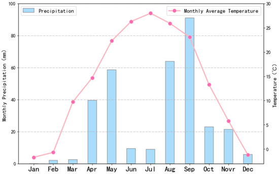
Figure 1.
Statistical map of temperature and precipitation data for Beijing in 2019.
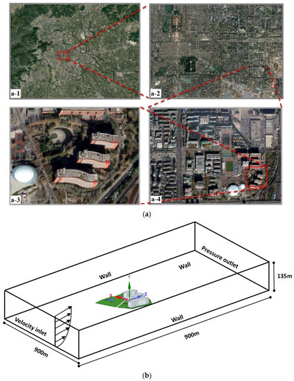
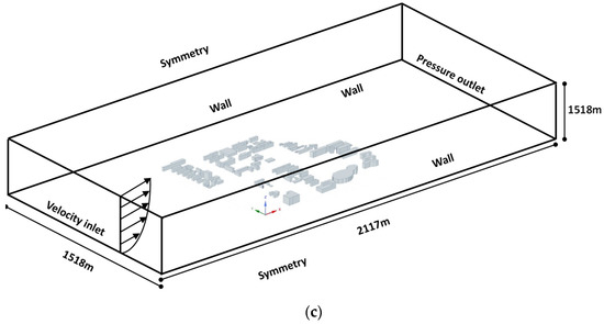
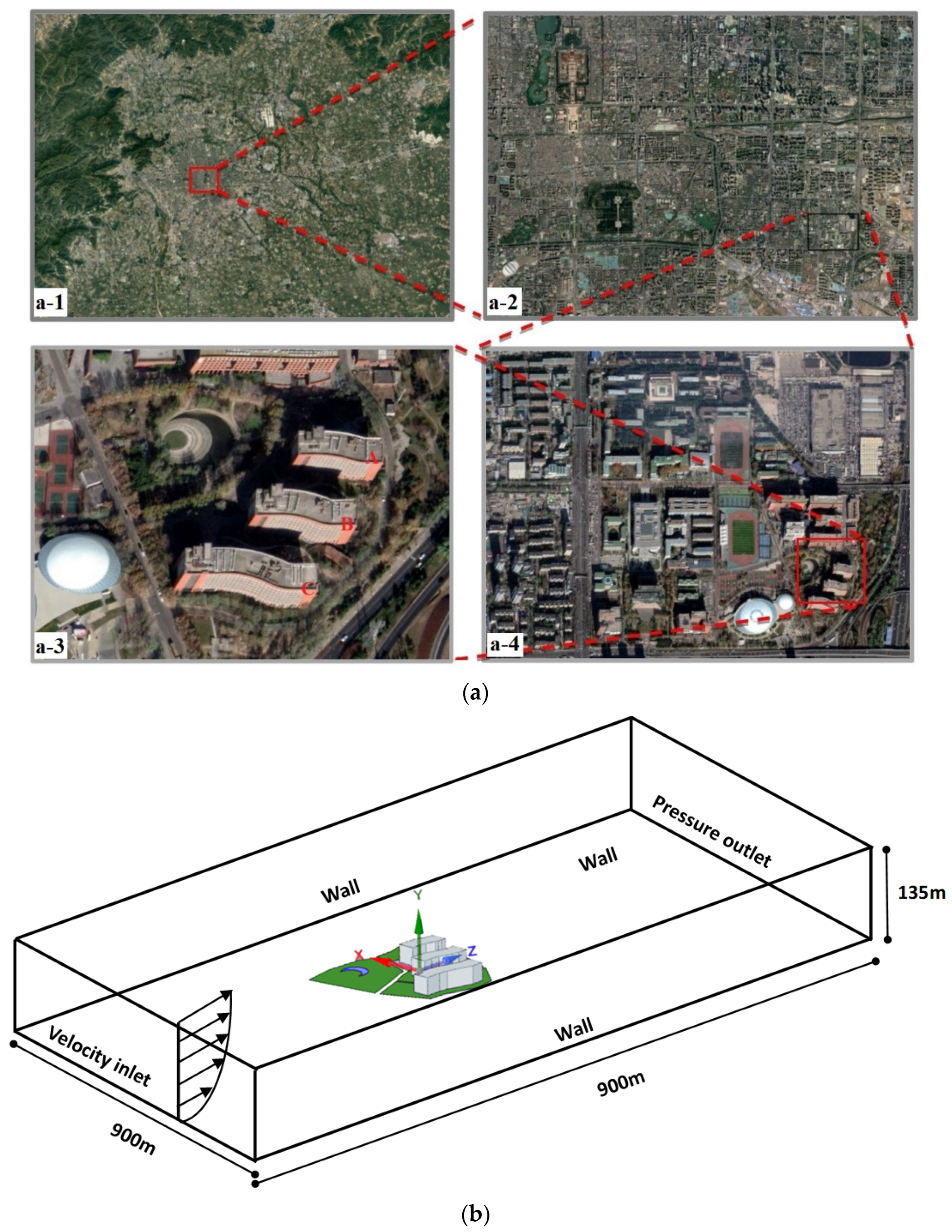
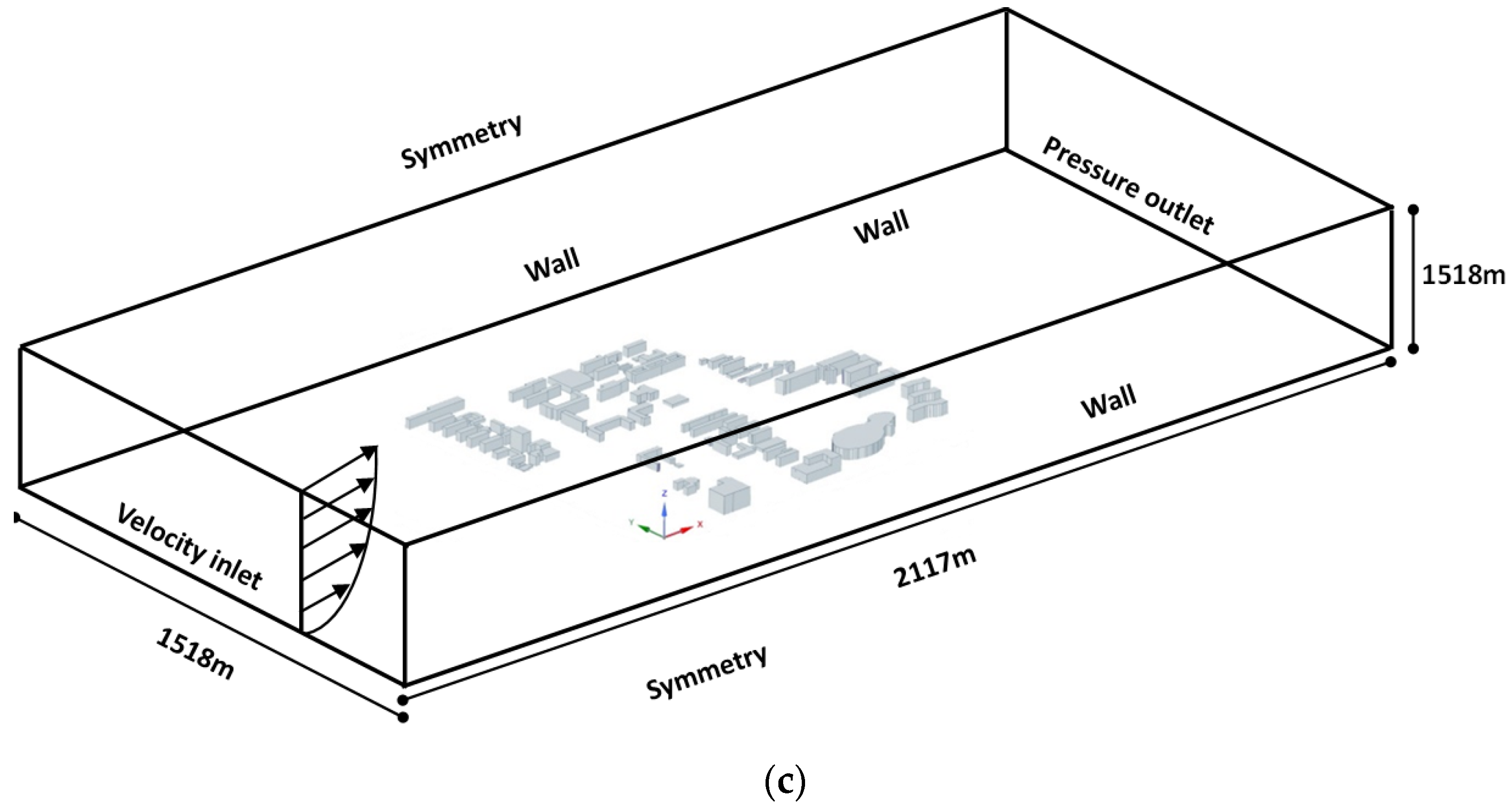
Figure 2.
High-resolution remote-sensing satellite image of the study area: (a) the physical model of the CFD calculations in the study area, and the size of its computational domain, (b) the geometric model of the campus of the Beijing University of Technology, and (c) the geometric model of three buildings at the southeast of the campus of the Beijing University of Technology.
In this study, multispectral images from the GaoFen-2 satellite were combined with remote-sensing images from the Google Earth satellite to divide the urban underlying surface of the study area into four components, including buildings, grasslands, water bodies, and roads. Based on the classification results, a 3D geometric model of each component was established using SpaceClaim 3D modeling software. In the study of the influence of changes in vegetation geometric characteristics on the thermal environment of the CFD simulation space, we chose three buildings, including the Ruanjian building (A in Figure 2(a-3)), the Chengjian building (B in Figure 2(a-3)), and the Shixun building (C in Figure 2(a-3)), of the university campus community as the CFD simulation objects, and we built the relevant geometric models (as shown in Figure 2b). In the research of simulating a space thermal environment at a community scale, a three-dimensional geometric model of the community building of the Beijing University of Technology was established, as shown in Figure 2c.
3. Materials and Methodology
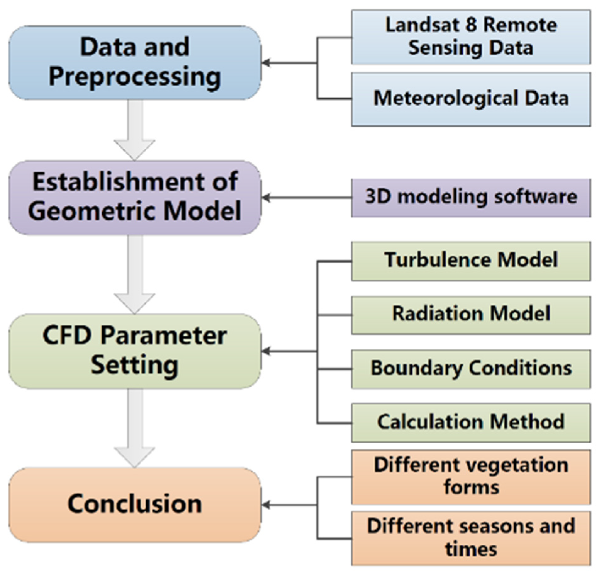
In this study, the dataset, including high-resolution, remotely sensed images and meteorological data, were preprocessed and used to build a three-dimensional (3D) geometric model. The parameters of the materials and the conditions of boundary were set, and the turbulence model, radiation model, and computational method were selected. Then, the wind speed profile and its calculation method were defined. The porous media model for vegetation was simplified, and the parameters of the model were also set. The flowchart of the study is shown in Figure 3.
Figure 3.
The flowchart of the study.
3.1. Materials and Their Processing
3.1.1. 3D Model Building Based on Remotely Sensed Dataset
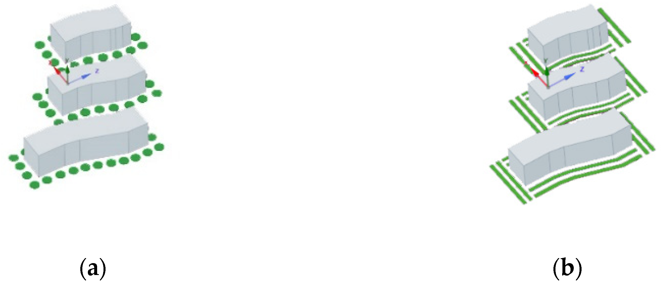
According to GaoFen-2 multispectral images and Google Earth remote-sensing images, a three-dimensional geometric model of the study area was established based on SpaceClaim, and a calculation area that met the relevant requirements of the CFD numerical simulation was set. According to the actual situation of the study area and the vegetation distribution characteristics of the surrounding buildings, four morphological characteristics of vegetation distribution were designed as dotted wrapping, ribbon wrapping, polyline wrapping, and arc wrapping. The modeling of the specific morphological layouts is shown in Figure 4. Based on CFD, the wind and heat environments of the urban construction, software, and training buildings of the community of the Beijing University of Technology under layouts of different vegetation patterns were simulated. The simulation research process was set under the same meteorological conditions and boundary conditions for the four different vegetation arrangements. In order to reduce the computational workload and simplify the generation of grids, some details of the buildings’ three-dimensional surfaces, such as balconies and shading components, were ignored in the simulation process.
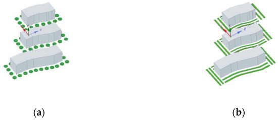
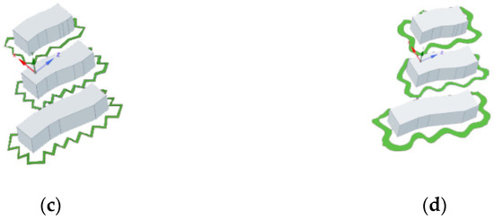
Figure 4.
Grass-building models with different geometric layouts: (a) dotted shape, (b) ribbon shape, (c) polyline shape, and (d) arc shape.
3.1.2. Definition of Materials
According to the remote-sensing images combined with field research, the underlying surface of the study area was divided into four elements, including trees, water bodies, buildings, and roads. Combining on-the-spot investigation and relevant architectural design materials, the building materials were described mainly as concrete, and the roads were mainly asphalt pavement. During the process of this simulation research, the relevant material properties of the underlying surface were set as shown in Table 1.

Table 1.
Physical properties of different underlying surface materials.
3.1.3. Meteorological Dataset
This study selected relevant meteorological data (including temperature, humidity, wind speed, wind direction, solar altitude, solar radiation, atmospheric visibility, etc.) that were used as the input conditions for the CFD space thermal environment simulation during both day and night in four seasons of spring, summer, autumn, and winter (data from the China Meteorological Administration; see Table 2). The solar radiation intensity could be obtained for a specific date by inputting the latitude and longitude information of the simulated area and the corresponding time zone into a solar calculator that came with the FLUENT software.
Table 2.
Meteorological data used to simulate the seasonal daytime and nighttime space air temperature and wind field.
3.2. CFD Modeling Principle
3.2.1. CFD Turbulence Governing Equations
The k-ε two-equation model is the most commonly used CFD model to simulate turbulence. The two-equation model is further divided into the standard k-ε model [43], the RNG k-ε model [44], and the realizable k-ε model [45]. RANS and realizable k-ε models can quickly characterize flow properties. However, under the solution of the nondesign point, convergence is difficult, the flow field structure cannot be accurately simulated, and a large amount of calculation is required. They require not only high spatial resolution to capture the flow structure, but also an accurate temporal description of the physical flow. Therefore, these two models are not suitable for simulating large separation flows. The standard k-ε turbulence model has high accuracy, a small fluctuation range, and requires less computation than the other two methods, so it is widely used in simulation research of urban thermal environments.
The governing equations of the standard k-ε turbulence model are as follows:
Continuity Equation:
Momentum Equation:
Turbulence Equation:
Energy Equation:
in which:
- ρ
- is the fluid density (unit is m3/s);
- t
- is time (unit is s);
- v
- is the speed vector (unit is m/s);
- p
- is the pressure on the infinite element (unit is N);
- τ
- is the viscous stress (unit is N);
- F
- is the volume (unit is m3);
- Cp
- is the thermal capacitance (unit is kJ·kg/°C);
- T
- is the temperature (unit is °C);
- k
- is the coefficient of heat conductivity (unit is W·m2/K);
- ST
- is the viscous dissipation term;
- ϕ
- is the flux variant;
- Γ
- is the general diffusion coefficient;
- S
- is the general source term.
3.2.2. Mesh Division and Boundary Condition Parameter Settings
In the meshing part, the ANSYS FLUENT MESH module was used to divide the computational domain into unstructured meshes. The boundary conditions of the computational domain are shown in Table 3. For the radiation model, the P1 radiation model was used in this paper as referenced in [46]. In this study, in order to reduce the number of grids and the amount of calculations, we simplified the real building into a wall with a certain thickness that participated in convective heat transfer and radiative heat transfer.
Table 3.
Boundary conditions and related parameter settings.
For simplicity, building walls, building roofs, and pavements were modeled as zero-thickness walls, where the heat conduction was calculated using a shell conduction model. Based on the solar radiation calculation module attached to the ANSYS FLUENT software, the total solar radiation, scattered solar radiation, and solar radiation vector were calculated. The P1 radiation model was used to solve for the radiative heat transfer, which is considered to be less computationally demanding and is, thus, widely used [42,47,48,49,50,51,52].
3.2.3. Calculation and Setting of Wind Speed Profile
The surface roughness of the urban boundary layer can significantly hinder the airflow. This effect can lead to large differences in wind speed with altitude. In order to make the simulation calculation of this study closer to the actual situation, in this paper the exponential wind profile velocity inlet was selected, and its calculation formula is shown in Equation (5) [24,47,48,49]:
where Hc is the reference height (m); VC is the speed at the reference height (m/s); and VH is the speed at height H (m/s). The value of the index α depends on objective factors, such as surface roughness, topography, vegetation, and spatial structure, and is independent of the wind speed. Referring to relevant standards, the indices for suburban terrain and large city centers range from around 0.28 to 0.40. Therefore, it was reasonable to take 0.3 in this study.
3.2.4. Simplification and Setting of Vegetation Porous Media Model
Increased vegetation greening is an important mitigation measure for urban spatial thermal environments, and it is also one of the hotspots in current research on spatial thermal environment mitigation measures. The mechanism of greenspace vegetation alleviating the heat island effect is mainly reflected in the following two aspects [35]. On one hand, vegetation absorbs part of the solar radiation through its own photosynthesis and then reflects part of the solar radiation through vegetation leaves [53]. The temperature difference caused by trees blocking solar radiation and absorbing energy can reach a maximum of 6 °C [36]. On the other hand, transpiration from vegetation absorbs most of the heat and converts it into a latent heat flux, which prevents the temperature from rising. The cooling effect of greenspace vegetation is based on different principles at different heights. At a height of 2 m, cooling is achieved by shading from solar radiation and latent heat exchange. At a height of 10m, it is achieved by heat exchange between vegetation and the atmosphere [1]. However, there are currently no parameters set specifically for vegetation models in CFD software. Li [1] and Liu [11] used Opening as the medium representing vegetation and used surface parameters retrieved with remote sensing (extracting greenspace evapotranspiration from the surface evapotranspiration map) to set the Opening medium model. Weak air flow was simulated to reflect the role of these underlying surfaces in the air flow.
The latest research shows that simplifying vegetation into a porous medium model and simulating the CFD flow field and temperature field could well reflect the influence of vegetation on wind speed and temperature in the environment [33]. This is achieved by dividing the tree into solid walls in the trunk part and porous air domains in the canopy part and assuming that the air domains absorb heat by volume. The airflow part can be represented by adding a source term to the CFD equation. The vegetation area is set as a porous medium, and the inertial drag coefficient and viscous drag coefficient are obtained using Darcy’s law [53].
The relevant formula is as follows:
Momentum source term:
Energy source terms absorbed by trees:
Turbulent kinetic energy Sk and turbulent dissipation rate Sε:
in which:
- ρa (kg/m3) is the density of air;
- Cd is the drag coefficient;
- LAD is the leaf area density;
- ui is the local speed in the i-direction;
- u is the magnitude of the local speed;
- Rn,vol (W/m3) is the volumetric net radiation;
- Qconv (W/m2) is the heat flux;
- LEv (J/kg) is the amount of latent heat released by leaves;
- Sk is the sink term of the turbulence kinetic energy equation;
- Sε is the sink term of the turbulent dissipation.
4. Results and Discussion
Regarding the aim of this study, the seasonal daytime and nighttime urban spatial 3D surface temperatures and air temperatures were simulated at a microscale, and the wind field information was also simulated based on meteorological datasets. Considering the mitigation effects of vegetation for urban canopy heat island, as well as that vegetation is also an effective and inexpensive way to alleviate urban spatial thermal environments, we carried out a study on spatial air temperature field distribution and wind fields, as well as the variation trends of different spatial layouts of vegetation, including dotted, ribbon, polyline, and arc layouts, designed based on real-area values. To further explore the relationship between urban landscape and air temperature, especially the relationship between the layout of construction buildings and the urban canopy heat island, we carried out a simulation of 3D surface and air temperatures and analyzed their relationship with the distribution and layout of buildings. We also analyzed the relationship between the spatial air temperature and the wind field distribution. Thus, the results are discussed based on these two aspects.
4.1. Simulation of 3D Urban Spatial Surface and Air Temperatures
4.1.1. Influence of Vegetation Morphology Layout on Temperature
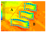
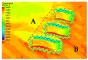
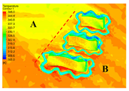
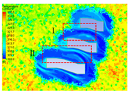
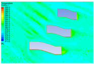
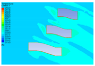
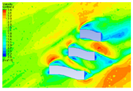
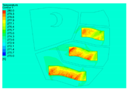
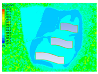
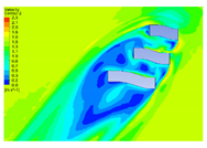
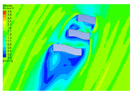
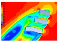
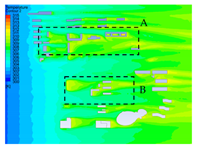
Table 4 shows the air temperature field distribution and its variation trends under different geometrical layouts of vegetation, including dotted, ribbon, polyline, and arc layouts of vegetation, simulated by CFD at heights of 0 m (land surface temperature), 2 m, 5 m, 10 m, and 20 m. In Table 4, at the height of 0 m, namely at land surface, shows the temperature distributions of buildings and ground surfaces under different vegetation layout forms. Under strong solar radiation in the summer, the surfaces of the earth and buildings received a large amount of solar radiation, which caused the surface temperature to rise rapidly. The vegetation maintained a lower temperature due to the absorption of solar radiation and transpiration by photosynthesis, which had a significant mitigation effect on the air temperature. This cooling effect affected the temperature distribution in the downwind direction under the action of the dominant southeasterly wind in summer. From the figure, the surface temperature in the downwind area (the upper left area A of the dashed line in Table 4) was significantly lower than that in the upwind area (the lower right area B in the dashed line).
Table 4.
The air temperature field distribution and its variation trends for dotted, ribbon, polyline, and arc layouts of vegetation under different geometrical layouts of vegetation simulated by CFD at heights of 2 m, 5 m, 10 m, and 20 m.
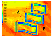
At the height of 2 m, Table 4 shows the distribution of the atmospheric temperature for different grassland morphological layouts at a distance of 2 m, or near the ground. At noon in the summer, the photosynthesis and transpiration of grassland vegetation had a certain impact on the atmospheric temperature, and the atmospheric temperature decreased. After comprehensive analysis, we believe that the possible reasons for the above results are mainly the following two: (1) Grassland absorbs a lot of solar radiation through the photosynthesis of leaves, and most of the energy is absorbed by the plants themselves. (2) The heat of the near-surface soil exchanges energy with the atmosphere, and the water in the soil is heated and vaporized into water vapor, which takes away a lot of energy.
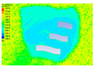
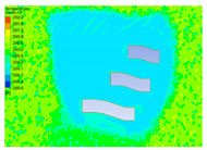
Comparing the temperature distribution at a height of 2 m with different vegetation forms, it can be seen that the mitigation effects of different forms of vegetation on temperature in the downwind direction were significantly different. This difference was mainly reflected in the areas between the buildings (areas I and II). Comparing the temperatures in areas I and II under different layout forms, it was found that the folded-line grassland layout had the most obvious mitigation effect on the temperature, followed by the strip layout. It can be seen from the figure below that the mitigation capabilities of vegetation with different layouts were: polyline > strip > point > arc.
Table 4 also shows the air temperature distribution under different grassland layouts at heights of 5 m, 10 m, and 20 m. A comprehensive comparative analysis showed that, at heights of 5 m, 10 m, and 20 m, the mitigation effect of vegetation on the spatial thermal environment was very weak, or even negligible. Different grassland layouts did not cause significant temperature differences. We speculated that the main reason could be that grassland is mainly distributed near the surface, and its mitigation effect needs to rely on the medium of airflow and then rely on the flow of wind to transmit this mitigation effect to other areas to achieve temperature regulation. However, under nonquiet wind conditions, the flow of wind tended to move in the horizontal direction, and at the vertical height, the atmospheric temperature at higher altitudes was less affected by the mitigation effect of vegetation. Therefore, the mitigation effect of vegetation was only reflected near the ground and had no obvious effect at high altitudes.
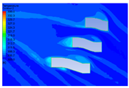
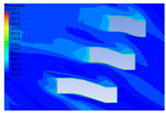
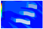
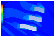
4.1.2. Influence of Vegetation Morphology Layout on Wind Speed
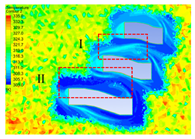
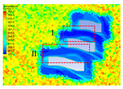
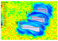
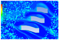
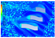
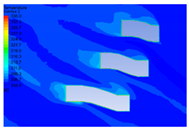
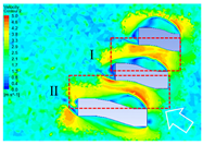
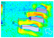
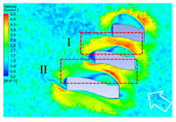
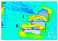
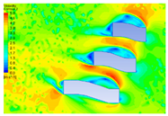
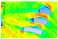
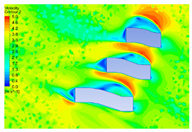
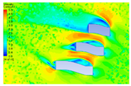
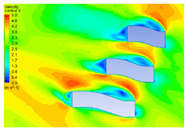
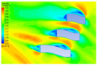
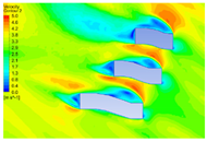
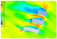
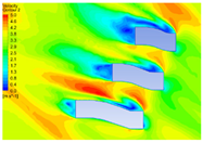
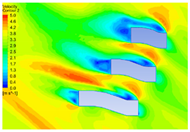
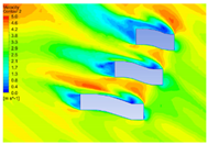
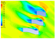
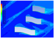
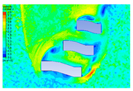
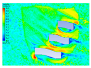
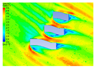
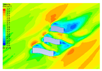
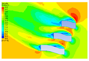
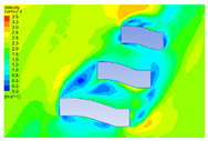
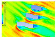
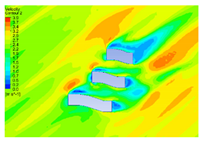
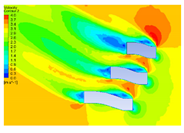
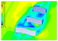
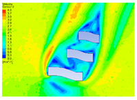
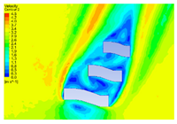
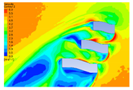
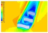
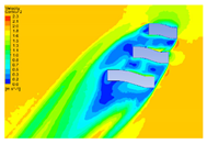
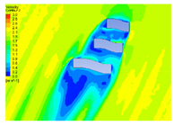
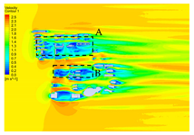
Different vegetation layouts have different blocking effects on airflow. The obstruction of airflow across vegetation surfaces increases with the surface roughness. When the surface is relatively smooth, there is less obstruction to the flow, and the air flow is smoother. This different degree of obstruction makes the airflow show characteristics of scattered distribution. Table 5 shows the wind speed distribution at the 2 m position under different vegetation layouts. It can be seen from the figure that, under the influence of the dominant southeast wind in the summer, there was a “narrow tube effect” between the buildings. This effect was more obvious on the north and south sides of the urban construction building, forming a local wind-speed-strengthening area. The maximum wind speed was close to 5 m/s, and the maximum wind speed area was mainly distributed in the corridors between the buildings (zones I and II).
Table 5.
The wind field distribution and its variation trends with dotted, ribbon, polyline, and arc layouts of vegetation under different geometrical layouts of vegetation simulated by CFD at heights of 2 m, 5 m, 10 m, and 20 m.
Due to the blocking effect of the buildings on the airflow, in the northeast corner and the west area of each building, the wind speed was lower than 1 m/s, and it was mainly distributed in the downwind direction of the building with the dominant wind direction. It can be seen in Table 5 that the high-wind-speed area of zone I in the belt-like distribution was the largest, followed by broken line > point > arc. The high wind speed in zone II was the largest, followed by point > arc > broken line.
4.1.3. Distribution Characteristics of Wind and Heat Environment during Daytime and Nighttime in Four Seasons
- (A)
- Distribution characteristics and analysis of wind and heat environment for daytime in four seasons
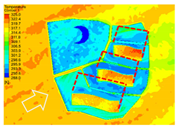
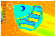
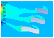
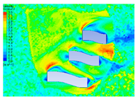
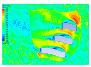
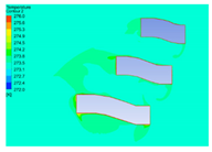
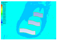
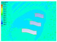
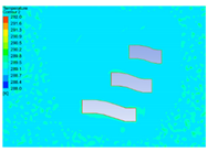
Table 6 shows the distributions of surface temperature and building surface temperature in different seasons based on different meteorological parameters. The results clearly show the difference that the vegetation and buildings made when they absorbed solar radiation during the day. Vegetation and water bodies kept the temperature at a low level due to their own physical properties, while the building surface absorbed solar radiation and increased its temperature rapidly. In addition, the temperature difference between building walls exposed to solar radiation and those not exposed to the sun (within the dashed line in Table 6) is also well-shown in the figure, and the surface temperature in the shaded area was significantly lower than that of the direct solar area surface. In the figure, we can clearly see the changes in the shaded area of the buildings at different sun altitudes due to the changes in the direct sunlight point in different seasons. In winter, the direct sunlight point was located near the Tropic of Cancer. At this time, the sun elevation angle was small, resulting in the largest shadow area in winter, followed by spring and autumn, and the smallest shadow area in summer.
Table 6.
The daytime surface and vertical air temperature distributions and their variation trends for spring (April), summer (July), autumn (October), and winter (January) simulated by CFD at heights of 0 m (land surface temperature), 2 m, 5 m, 10 m, and 20 m.
The surface temperatures were lower in sunless areas shaded by buildings. This showed that, in the summer, solar radiation is the most important factor causing the increase in surface temperature. Especially on the sunny side of the buildings, due to the repeated reflection and absorption of the long-wave radiation in solar radiation on the ground and the sunny side of the building, the ground temperature near the sunny side was significantly higher than the other surfaces.
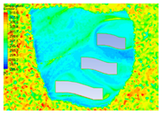
Table 7 shows the distribution of atmospheric temperature in the four seasons during daytime at 2 m near the ground. The photosynthesis and transpiration of grassland vegetation had a certain influence on the atmospheric temperature, and the atmospheric temperature decreased. This effect was concentrated near the surface and had less effect on high air temperatures at higher altitudes. The roads experienced significant heat flow and heat build-up after being exposed to solar radiation. Among them, the wall temperature difference between the sunny side and the back side of the buildings is also well-reflected in the figure.
Table 7.
The daytime wind field distributions corresponding to temperature distributions (see Table 6) and their variation trends for spring (April), summer (July), autumn (October), and winter (January) simulated by CFD at heights of 2 m, 5 m, 10 m, and 20 m.
- (B)
- Distribution characteristics and analysis of wind and heat environment for night time in four seasons
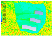
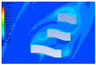
It can be seen from the nighttime surface temperature distribution diagram shown in Table 8 that the surface temperature difference of different objects was smaller than that in the daytime, the temperature distribution was more stable, and the variation range was smaller. We believe that there were two main reasons for this result. On one hand, because night is not affected by solar radiation, the temperature difference mainly comes from heat conduction of the indoor temperature through building walls and air-layer heat convection between building walls and near walls (Table 8). On the other hand, when vegetation enters the respiration stage at night, the effect of vegetation on air temperature is negligible. At this time, the main source of heat is the interior of buildings and artificial heat.
Table 8.
The nighttime surface and vertical air temperature distributions and their variation trends for spring (April), summer (July), autumn (October), and winter (January) simulated by CFD at heights of 0 m (land surface temperature), 2 m, 5 m, 10 m, and 20 m.
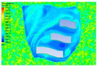
In the downwind direction of the buildings, some heat on the building surfaces was convective heat transferred through the air near the walls. This phenomenon was more obvious in spring, summer, and autumn (Table 9; at the height of 0 m). However, it is worth mentioning that the efficiency of this heat exchange is relatively low, mainly because most current building walls use thermal insulation materials. Therefore, even if there is an exchange of heat, it is difficult to make a significant difference in the air temperature. What is shown in the result graphs (Table 9; at heights of 2 m, 5 m, 10 m, and 20 m) is that the air temperature distribution around the buildings was quite stable at different heights, and the difference was not obvious, especially at night in the winter. Therefore, the regularity reflected in the temperature distribution map was not obvious.
Table 9.
The nighttime wind field distributions and corresponding temperature distributions (see Table 7) and their variation trends for spring (April), summer (July), autumn (October), and winter (January) simulated by CFD at heights of 2 m, 5 m, 10 m, and 20 m.
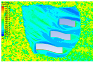
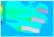
4.2. Simulation of Urban Wind and Heat Environment and Research on Its Distribution Characteristics at a Community Scale
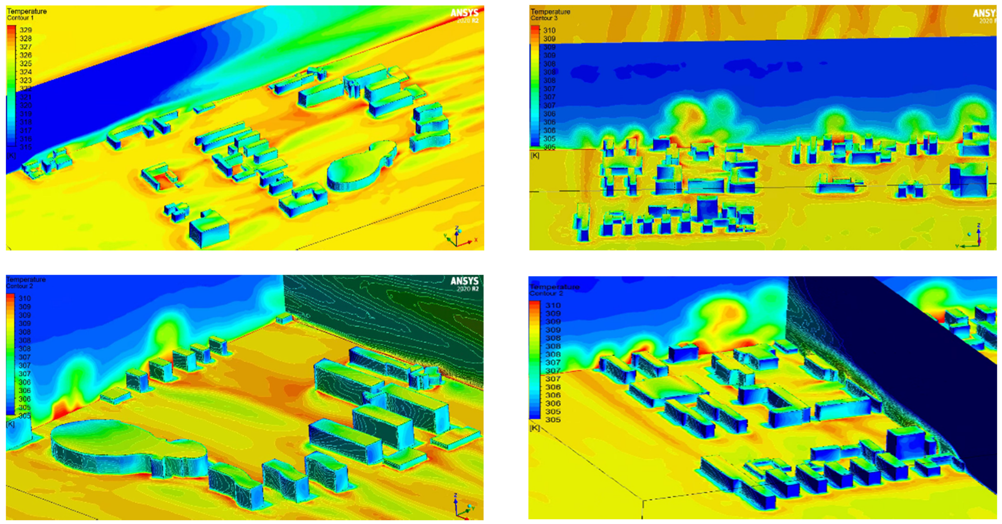
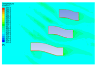
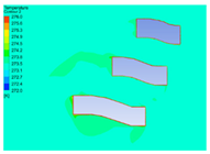
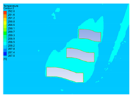
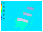
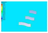
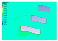
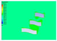
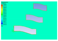
The distribution of wind and thermal environments for different morphological arrangements of daytime and nighttime vegetation at a microscopic scale was discussed above. However, the community scale is the main activity area of residents, and the spatial air–heat environment and thermal comfort at the community scale are more closely related to residents’ lives. Therefore, it is very necessary to simulate spatial wind and heat environments at the community scale. Urban structure layout greatly affects the urban heat island effect. Based on CFD and considering factors such as building layout, building number, building density, and building aspect ratio, simulating wind and heat environments at both the micro-scale and the community scale is of great significance for optimizing comprehensive urban design, as well as improving the urban landscape and ecological environment. In urban planning, it is necessary to rationally arrange building interval and orientation in combination with meteorological conditions so that the building orientation conforms to the prevailing wind direction. This can increase the ventilation of buildings so that the urban heat distribution is more even and reasonable. It is of great significance to alleviating the heat island effect. This section mainly analyzes the distribution and influence of building layout at the community scale on urban spatial wind and heat environments at different heights in different seasons. Figure 5 and Figure 6 show the 3D urban spatial air temperature profiles simulated based on CFD. In Figure 5, some air temperature profiles are selected as examples to illustrate that the 3D atmospheric temperature in the vertical direction of air could be successfully simulated based on CFD. In Figure 6, 3D spatial air temperature profiles on a vertical plane parallel to the wind direction and air temperature profiles on the vertical plane perpendicular to the wind direction are introduced. The results show that the spreading direction of the simulated air temperature and the effects of the layout of buildings on canopy heat island could be clearly addressed. To explicitly explore the influence of building geometry and layout on the 3D air temperature field, the results of the land surface temperature; the 2 m, 5 m, 10 m, and 20 m air temperatures; the wind field; and the wind pressure were introduced to make a comparative analysis.
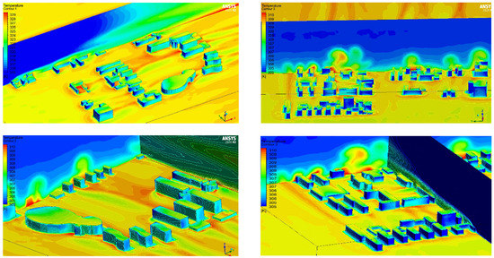
Figure 5.
Air temperature profiles in a vertical direction simulated based on CFD.
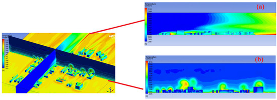
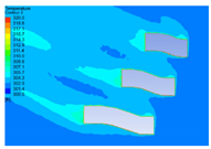
Figure 6.
Daytime 3D spatial air temperature profiles in a vertical direction: (a) the air temperature profile on a vertical plane parallel to the wind direction and (b) the air temperature profile on a vertical plane perpendicular to the wind direction.
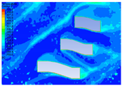
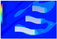
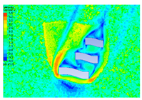
4.2.1. Distribution Characteristics and Influencing Factors of Spatial Wind and Heat Environment at a Community Scale during the Daytime
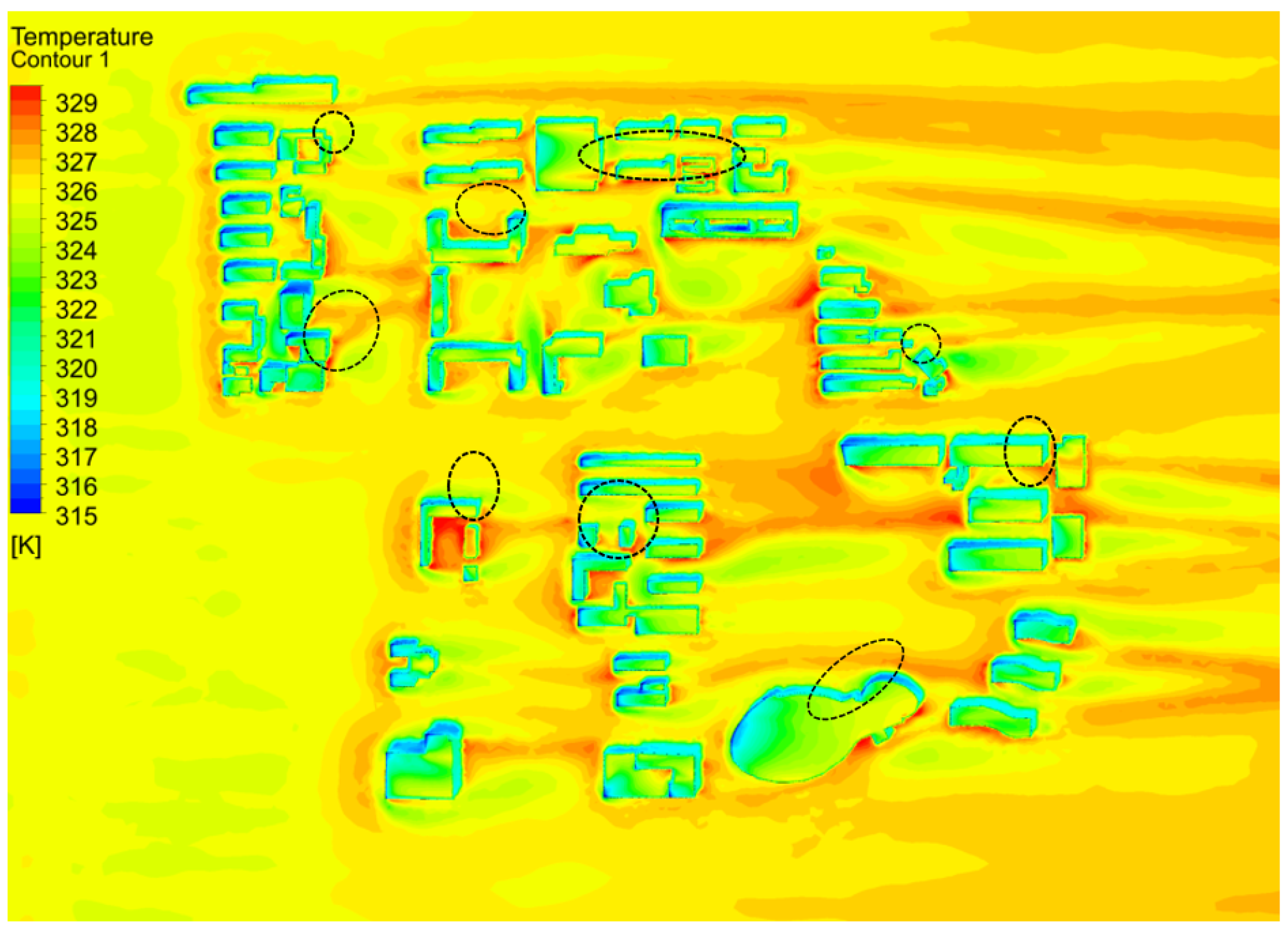
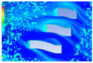
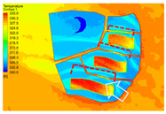
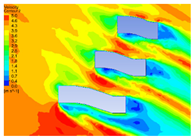
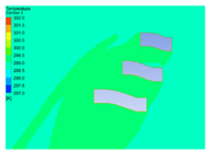
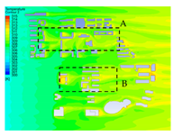
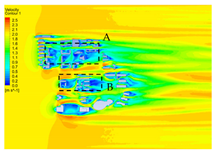
Figure 7 shows the simulated building surface temperatures and land surface temperatures of the Beijing University of Technology campus in the summer. Figure 7 clearly shows that the buildings blocked the sun’s rays, resulting in temperature differences between the ground surfaces. In addition, it can also be seen in Figure 6 that the temperature in the upwind direction was significantly lower than the temperature in the downwind direction on the building surfaces and the ground surface. This was mainly due to the obvious convective heat transfer between the building surfaces and the atmosphere. Conversely, the surface temperature was higher in the downwind direction and in the area blocked by the building (shown within the dashed line in Figure 7).
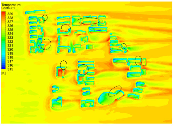
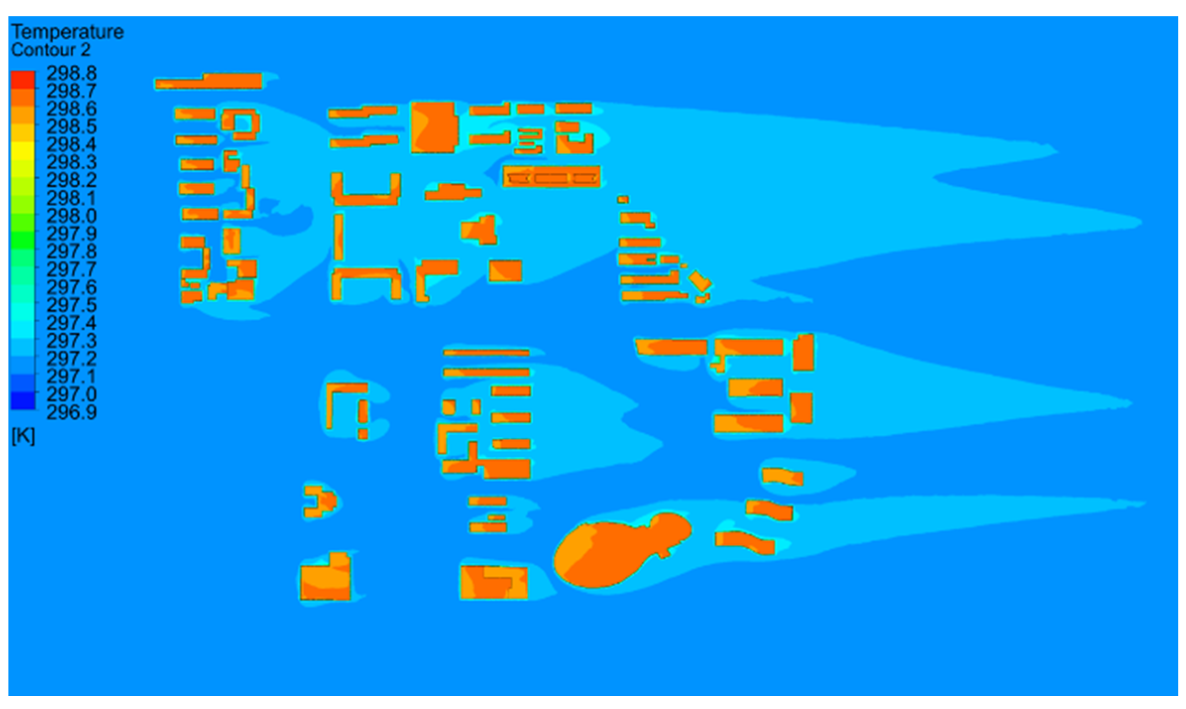
Figure 7.
The daytime surface temperature field distribution and variation trend simulated by CFD.
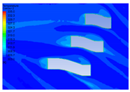
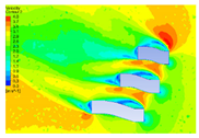
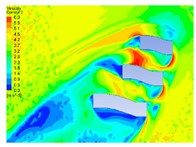
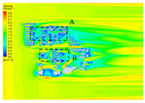
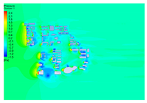
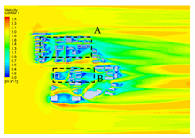
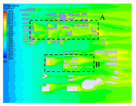
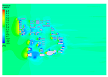
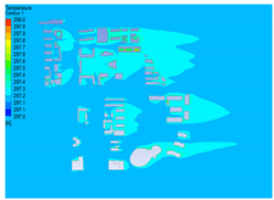
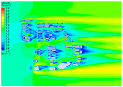
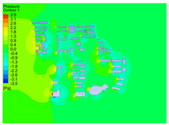
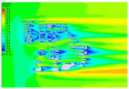
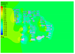
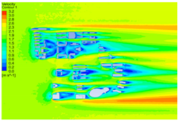
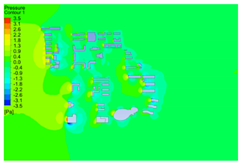
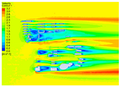
Table 10 shows the temperature distribution, wind speed, and wind pressure distribution at 2 m, 5 m, 10 m, and 20 m of the Beijing University of Technology campus. Combining the results for the wind environment and thermal environment, it can be seen that the distribution of temperature had a great correlation with the direction of wind. Areas A and B for the daytime wind field results had lower wind speeds in the downwind direction due to the blocking of buildings, so the temperature in Table 10 is higher. The temperature was lower where the wind speed was higher, and the temperature was higher where the wind speed was lower. This was because the heat build-up in areas with lower wind speeds resulted in higher local temperatures, while areas with higher wind speeds could dissipate the accumulated heat well. This showed that convective heat transfer plays a leading role in the study of urban space thermal environments.
Table 10.
The daytime 3D urban spatial air temperature, wind field distribution, and wind pressure distribution with corresponding variation trends at heights of 2 m, 5 m, 10 m, and 20 m simulated by CFD.
In Table 10, under the action of the breeze, the building’s blocking effect on the wind made the wind speed on the leeward side of the building lower, and the wind speed value was below 1 m/s. However, the wind speed was not as large as possible. When the wind speed is greater than 5 m/s, the comfort of the human body in the wind environment decreases. It is worth mentioning that, in summer, an appropriate wind speed can dissipate heat very well, which can take away the heat accumulated around buildings and reduce the surrounding temperature significantly.
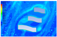
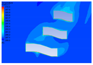
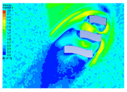
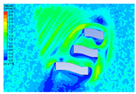
4.2.2. Distribution Characteristics and Influencing Factors of Spatial Wind and Heat Environment at the Community Scale at Nighttime
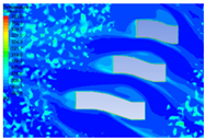
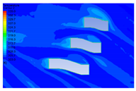
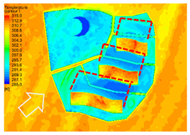
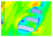
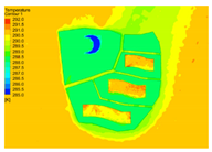
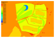
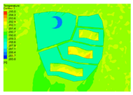
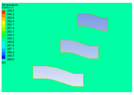
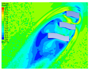
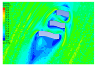
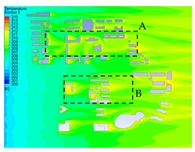
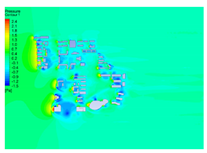
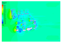
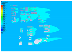
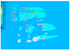
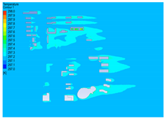
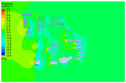
Figure 8 shows the simulation results of the surface temperature at nighttime on the campus of the Beijing University of Technology. It can be seen from the figure that the surface temperature map obtained by the simulation had a higher temperature on the building surfaces, while the other surface temperatures were lower. The surface temperature on the leeward side of the building was lower than on the other surface areas. Table 11 shows the nighttime temperature distributions at different heights on the campus of the Beijing University of Technology. In general, the temperature distributions at different heights at night did not show obvious differences, and the temperature variation range was small. Due to indoor heat transfer, the temperature in the densely built area was higher than that in the sparsely built area. Table 11 also shows the wind environment and wind pressure distribution at night on the campus of the Beijing University of Technology. The wind environment and wind pressure distribution were similar for night and day, and there was no obvious difference.

Figure 8.
The nighttime surface temperature field distribution and variation trend simulated by CFD.
Table 11.
The nighttime 3D urban spatial air temperature, wind field distribution, and wind pressure distribution with corresponding variation trends at heights of 2 m, 5 m, 10 m, and 20 m simulated by CFD.
Comparing the temperature maps in Table 10 and Table 11, it was found that the daytime temperature difference in the building-intensive area was larger than the nighttime temperature difference, and the temperature diffusion rate in the local building-concentrated area was slow, which had a certain impact on the surrounding background features. This was mainly due to the fact that the wind speed in the concentrated building area was affected by the roughness of the underlying surface. Judging from the distance of the building layout, there was a certain distance between different buildings, which had a certain positive impact on the wind speed and temperature and accelerated the speed of heat dissipation. From the perspective of wind pressure, the wind pressure at night was more stable than the wind pressure during the day, but the wind pressure value at night was larger, and the pressure difference was larger. Analyzing the layout of the buildings from the perspective of ventilation performance, it can be found from Table 10 and Table 11 that the staggered distribution of buildings affected the wind speed and wind pressure and had a certain blocking effect on the diffusion of building energy storage. The main wind direction and wind speed during the period when the heat island effect was the largest and the reasonable spacing and distribution of the buildings formed a ventilation corridor that was beneficial to heat dissipation.
In this study, through the analysis of the simulation results and data processing, it was found that there were still some problems that could affect the accuracy of the simulation results: (1) In the construction and simplification of the geometric physical model, subtle changes in the building surfaces, such as the arrangement of windows, doors, and roof structures, were ignored. We simplified the actual building as a building wall, introduced it into the CFD, and set it as concrete of a certain thickness to participate in the simulation calculation, ignoring the influence of the actual difference in the building surface on the results. (2) The CFD numerical simulation calculation ignored the wall temperature difference caused by the heat exchange inside the building. There were actually different types of underlying surfaces in the surface model, such as roads made of asphalt, squares made of concrete, and exposed soil, but these were reduced to a single underlying surface type. (3) There were also the limitations of the standard k-ε turbulence model and the P1 radiation model.
It is worth pointing out that, in the process of finite element simulation, the simplification processing and meshing of the model consume a lot of computation and time. Therefore, the work on model simplification and mesh division needs to be paid enough attention in the process of finite element simulation, including pre-processing, solver calculation, and post-processing. Unlike structural simulation, fluid mechanics simulation is characterized by a huge number of meshes. Therefore, it is necessary to make a trade-off in meshing the points of interest with a denser number of meshes to capture finer details, while the number of meshes for noninterest points can be smaller to reduce the computational consumption. In model processing, according to the subject studied, the geometric features of the subject model are described in detail, and the geometric models in other areas can be simplified and modified appropriately.
4.3. Thermal Environment Simulation Validation Based on Meteorological Station Observation Data
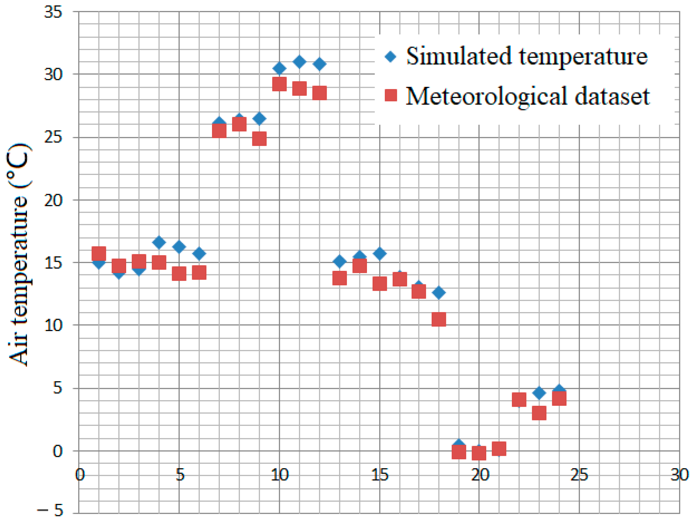
In this paper, the air temperature data obtained from the three meteorological stations closest to the distribution of the study area were used for comparison with the air temperature data obtained through the simulation to validate the accuracy of the simulated results. The temperatures of the four seasons and the simulated working conditions of day and night were mainly compared, and the comparison results are shown in the following figure. The simulation results for daytime and nighttime in different seasons were compared with the meteorological station data at the corresponding times, and the results are shown in Figure 9. It can be seen from the figure that the data obtained from the simulation were basically consistent with the measured data, and the maximum deviation occurred during the daytime in summer, which was about 2 °C. During the day, the simulated air temperature was higher than the measured air temperature. At night, the simulated and measured data were not compared, and there was no obvious pattern.
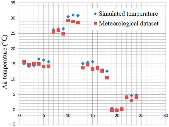
Figure 9.
Validation for simulated results based on meteorological dataset.
In this study, the air temperature data collected from three meteorological stations near the study area were compared with the air temperature data obtained through the simulation. The temperatures in the four seasons and the simulated working conditions of day and night were mainly compared. The results showed that the CFD method had good applicability to simulate urban thermal environments in the four seasons and the daytime. The root mean square error (RMSE) of the measured data and simulated data was calculated, as shown in Table 12. A comprehensive analysis of the errors in the simulation results of the daytime and nighttime temperature fields showed that the RMSE in the daytime was greater than that at night, which was mainly due to the greater influence of solar radiation on temperature differences during the day. During the day, the temperature difference between the summer and spring was greater than that of the autumn and winter. At night, the difference was greatest in the autumn and smallest in the spring and winter. The reasons for the seasonal differences we analyzed could be caused by the following aspects: (1) the different solar altitude angles and solar radiation intensities for different seasons, (2) the different influence of vegetation in different seasons (the influence of leaves in autumn and winter), or (3) the emission of anthropogenic heat, especially the influence of indoor heating, in the winter.
Table 12.
The validation for the simulated results based on three groups of meteorological datasets close to the study area.
5. Conclusions
Based on CFD, the numerical simulation results of an urban thermal environment at both daytime and nighttime under different vegetation forms and different seasons had high accuracy. Using the CFD method to study the urban space wind and heat environment, as well as to analyze its changing trend, had a better performance and a high accuracy for exploring the heat conduction mechanism between different components of the urban underlying surface and the influence mechanism of different layout forms on the spatial thermal environment.
From the simulation results, the temperature in the upwind direction of the dominant wind was lower than that after passing through vegetation, indicating that vegetation plays an important role in the mitigation effect of the thermal environment. However, different vegetation forms had different impacts on the urban thermal environment. The comparative analysis showed that the mitigation abilities from strong to weak of different forms of vegetation to the spatial thermal environment were in the order of broken line, strip, point, and arc. Different forms of vegetation also had different effects on the wind environment. The comfort level of the wind environment from high to low was belt, point, arc, and polyline. The characterization of the urban thermal environment in different seasons was in line with the climate conditions of the four seasons. The numerical simulations of the four seasons during the day clearly reflected the temperature difference caused by the change of the solar altitude angle with the seasons, as well as the temperature difference between the direct solar surface and the shadow surface. In the thermal environment simulations of the four seasons, it was found that the thermal environment performance at night was smaller than that of the daytime temperature, and the overall temperature performance of the region was relatively stable.
In the simulation results of the spatial thermal environment of the campus of the Beijing University of Technology at the community scale, it was found that there was a certain correlation between the variation trends of air temperature and wind speed. Heat transfer was one of the important ways to cause differences in the thermal environment of a space. By analyzing the simulation results at the community scale, it was found that the layout, number, and density of the buildings were closely related to the distribution of the thermal environment in the space. Areas with a large number of buildings and high density had large changes in wind speed and pressure and a high space temperature, which was not conducive to the diffusion of heat. The layout of the buildings also affected heat conduction and convection, so it is also extremely important to consider the relationship of building layouts to prevailing wind direction.
The results of this study showed that the integration of computational fluid dynamics and remote-sensing technology could be used to simulate urban 3D spatial wind and heat environments at various scales. Through the comparison and verification of the temperature data collected through meteorological data and the temperature data obtained from the simulation, it was seen that CFD and remote sensing are becoming powerful technical means for the simulation of urban wind and heat environments with relatively high accuracy. The simulation of urban wind and heat environments based on this method is of great importance for reasonable urban planning, building layout, and the low-carbon construction of green buildings.
The essence of CFD simulations of urban space wind and heat environments is to solve the partial differential governing equation of heat absorption and transfer by different underlying surface types under the action of solar radiation by each solution unit in the calculation space. The accuracy of CFD technology based on a finite difference method to simulate urban three-dimensional space wind and heat environments depends on the number of input parameters and their accuracy. These parameters include: (1) the underlying surface data of different thermophysical properties that cause differences in solar radiation heat; (2) meteorological boundary condition data, such as the temperature and wind speed in a study area; and (3) high-quality grid data for the study area through numerical computing technology. It is the limitations of these data and grid techniques that limit the application of this method to micro-scale and block-scale studies, with fewer simulations at the macro-scale. For the macroscopic scale, the research area is large: on one hand, the classification of the underlying surface and the geometric modeling of the three-dimensional space are difficult; on the other hand, grid division is difficult, and the number of grids is large, which requires a huge amount of calculation. In view of these limitations and difficulties, the following methods can also be used in macro-scale urban 3D spatial wind and heat environment simulations: the comprehensive use of multisource remote-sensing data to classify the underlying surfaces and to classify underlying surfaces with the same heat transfer properties and the performance of clustering and merging processing, which is beneficial to the simplification of the underlying surface and the three-dimensional space modeling. Based on the similarity criterion of fluid mechanics, the scale modeling of a study area can significantly reduce the number of grids and reduce the need for CFD calculation memory requirements, which can, in turn, significantly reduce the amount of computation.
Author Contributions
Conceptualization, H.H.; methodology, H.H. and F.C.; software, F.C.; validation, H.H. and F.C.; formal analysis, H.H. and F.C.; investigation, H.H. and F.C.; resources, F.C.; data curation, H.H. and F.C.; writing—original draft preparation, H.H. and F.C.; writing—review and editing, H.H.; visualization, F.C.; supervision, H.H.; project administration, H.H.; funding acquisition, H.H. All authors have read and agreed to the published version of the manuscript.
Funding
This research and the APC were funded by the Scientific Research Project of Beijing Municipal Educational Commission (grant number KM202110005017) and by the National Natural Science of Foundation of China (grant number 41701425).
Data Availability Statement
Not applicable.
Acknowledgments
Thanks for the funding from the State Key Laboratory of Media Convergence Production Technology and Systems, Beijing 100803, China.
Conflicts of Interest
The authors declare no conflict of interest.
References
- Li, K.; Yu, Z. Comparative and Combinative Study of Urban Heat island in Wuhan City with Remote Sensing and CFD Simulation. Sensors 2008, 8, 6692–6703. [Google Scholar] [CrossRef]
- Radhi, H.; Fikry, F.; Sharples, S. Impacts of urbanisation on the thermal behaviour of new built up environments: A scoping study of the urban heat island in Bahrain. Landsc. Urban Plan. 2013, 113, 47–61. [Google Scholar] [CrossRef]
- Dimoudi, A.; Zoras, S.; Kantzioura, A.; Stogiannou, X.; Kosmopoulos, P.; Pallas, C. Use of cool materials and other bioclimatic interventions in outdoor places in order to mitigate the urban heat island in a medium size city in Greece. Sustain. Cities Soc. 2014, 13, 89–96. [Google Scholar] [CrossRef]
- Takahashi, K.; Yoshida, H.; Tanaka, Y.; Aotake, N.; Wang, F. Measurement of thermal environment in Kyoto city and its prediction by CFD simulation. Energy Build. 2004, 36, 771–779. [Google Scholar] [CrossRef]
- Huo, H.; Chen, F.; Geng, X.; Tao, J.; Liu, Z.; Zhang, W.; Leng, P. Simulation of the Urban Space Thermal Environment Based on Computational Fluid Dynamics: A Comprehensive Review. Sensors 2021, 21, 6898. [Google Scholar] [CrossRef]
- Wong, K.; Paddon, A.; Jimenez, A. Review of World Urban Heat Islands: Many Linked to Increased Mortality. J. Energy Resour. Technol. 2013, 135, 022101. [Google Scholar] [CrossRef]
- Fan, H.; Sailor, D. Modeling the impacts of anthropogenic heating on the urban climate of Philadelphia: A comparison of implementations in two PBL schemes. Atmos. Environ. 2005, 39, 73–84. [Google Scholar] [CrossRef]
- Yao, Y.; Chen, X.; Qian, J. Research progress on the thermal environment of the urban surfaces. Acta Ecol. Sin. 2018, 38, 1134–1147. [Google Scholar]
- Sobrino, J.A.; Raissouni, N.; Li, Z.L. A comparative study of land surface emissivity retrieval from NOAA data. Remote Sens. Environ. 2001, 75, 256–266. [Google Scholar] [CrossRef]
- Li, Z.L.; Tang, B.H.; Wu, H.; Ren, H.; Yan, G.; Wan, Z.; Trigo, I.F.; Sobrino, J.A. Satellite-derived land surface temperature: Current status and perspectives. Remote Sens. Environ. 2013, 131, 14–37. [Google Scholar] [CrossRef] [Green Version]
- Liu, Z.; Wu, P.; Duan, S.; Zhan, W.; Ma, X.; Wu, Y. Spatiotemporal reconstruction of land surface temperature derived from fengyun geostationary satellite data. IEEE J. Sel. Top. Appl. Earth Obs. Remote Sens. 2017, 10, 4531–4543. [Google Scholar] [CrossRef]
- Duan, S.B.; Li, Z.L.; Li, H.; Göttsche, F.M.; Wu, H.; Zhao, W.; Leng, P.; Zhang, X.; Coll, C. Validation of Collection 6 MODIS land surface temperature product using in situ measurements. Remote Sens. Environ. 2019, 225, 16–29. [Google Scholar] [CrossRef] [Green Version]
- Qian, Y.; Wang, N.; Li, K.; Wu, H.; Duan, S.; Liu, Y.; Ma, L.; Gao, C.; Qiu, S.; Tang, L.; et al. Retrieval of surface temperature and emissivity from ground-based time-series thermal infrared data. IEEE J. Sel. Top. Appl. Earth Obs. Remote Sens. 2020, 13, 284–292. [Google Scholar] [CrossRef]
- Radhi, H.; Sharples, S.; Assem, E. Impact of urban heat islands on the thermal comfort and cooling energy demand of artificial islands—A case study of AMWAJ Islands in Bahrain. Sustain. Cities Soc. 2015, 19, 310–318. [Google Scholar] [CrossRef]
- Huang, J.-M.; Chen, L.-C. A Numerical Study on Mitigation Strategies of Urban Heat Islands in a Tropical Megacity: A Case Study in Kaohsiung City, Taiwan. Sustainability 2020, 12, 3952. [Google Scholar] [CrossRef]
- Kubilay, A.; Derome, D.; Carmeliet, J. Coupled numerical simulations of cooling potential due to evaporation in a street canyon and an urban public square. J. Phys. Conf. Ser. 2019, 1343, 012016. [Google Scholar] [CrossRef]
- Hsieh, C.-M.; Huang, H.-C. Mitigating urban heat islands: A method to identify potential wind corridor for cooling and ventilation. Comput. Environ. Urban Syst. 2016, 57, 130–143. [Google Scholar] [CrossRef]
- Tominaga, Y.; Sato, Y.; Sadohara, S. CFD simulations of the effect of evaporative cooling from water bodies in a micro-scale urban environment: Validation and application studies. Sustain. Cities Soc. 2015, 19, 259–270. [Google Scholar] [CrossRef]
- Toparlar, Y.; Blocken, B.; Maiheu, B.; van Heijst, G. A review on the CFD analysis of urban microclimate. Renew. Sustain. Energy Rev. 2017, 80, 1613–1640. [Google Scholar] [CrossRef]
- Albatayneh, A.; Alterman, D.; Page, A. Adaptation the use of CFD modelling for building thermal simulation. In Proceedings of the 2018 International Conference on Software Engineering and Information Management, Casablanca, Morocco, 4–6 January 2018; pp. 68–72. [Google Scholar]
- Antoniou, N.; Montazeri, H.; Neophytou, M.; Blocken, B. CFD simulation of urban microclimate: Validation using high-resolution field measurements. Sci. Total Environ. 2019, 695, 133743. [Google Scholar] [CrossRef]
- Ashie, Y.; Kono, T. Urban-scale CFD analysis in support of a climate-sensitive design for the Tokyo Bay area. Int. J. Clim. 2010, 31, 174–188. [Google Scholar] [CrossRef]
- Chang, S.; Jiang, Q.; Zhao, Y. Integrating CFD and GIS into the development of urban ventilation corridors: A case study in Changchun City, China. Sustainability 2018, 10, 1814. [Google Scholar] [CrossRef] [Green Version]
- Du, H.; Cai, Y.; Zhou, F.; Jiang, H.; Jiang, W.; Xu, Y. Urban blue-green space planning based on thermal environment simulation: A case study of Shanghai, China. Ecol. Indic. 2019, 106, 105501. [Google Scholar] [CrossRef]
- Piroozmand, P.; Mussetti, G.; Allegrini, J.; Mohammadi, M.H.; Akrami, E.; Carmeliet, J. Coupled CFD framework with mesoscale urban climate model: Application to microscale urban flows with weak synoptic forcing. J. Wind. Eng. Ind. Aerodyn. 2020, 197, 104059. [Google Scholar] [CrossRef]
- van Hooff, T.; Blocken, B.; Tominaga, Y. On the accuracy of CFD simulations of cross-ventilation flows for a generic isolated building: Comparison of RANS, LES and experiments. Build. Environ. 2017, 114, 148–165. [Google Scholar] [CrossRef]
- Fatima, S.F.; Chaudhry, H.N. Steady-state CFD modelling and experimental analysis of the local microclimate in Dubai (UAE). Sustain. Build. 2017, 2, 5. [Google Scholar] [CrossRef] [Green Version]
- Zhang, Y.; Zhan, Y.; Yu, T.; Ren, X. Urban green effects on land surface temperature caused by surface characteristics: A case study of summer Beijing metropolitan region. Infrared Phys. Technol. 2017, 86, 35–43. [Google Scholar] [CrossRef]
- Tominaga, Y.; Mochida, A.; Okaze, T.; Sato, T.; Nemoto, M.; Motoyoshi, H.; Nakai, S.; Tsutsumi, T.; Otsuki, M.; Uamatsu, T.; et al. Development of a system for predicting snow distribution in built-up environments: Combining a mesoscale meteorological model and a CFD model. J. Wind. Eng. Ind. Aerodyn. 2011, 99, 460–468. [Google Scholar] [CrossRef]
- Antoniou, N.; Montazeri, H.; Wigo, H.; Neophytou, M.K.-A.; Blocken, B.; Sandberg, M. CFD and wind-tunnel analysis of outdoor ventilation in a real compact heterogeneous urban area: Evaluation using “air delay”. Build. Environ. 2017, 126, 355–372. [Google Scholar] [CrossRef]
- Mirzaei, P.A.; Haghighat, F. Approaches to study Urban Heat Island—Abilities and limitations. Build. Environ. 2010, 45, 2192–2201. [Google Scholar] [CrossRef]
- Gülten, A.; Aksoy, U.T.; Öztop, H.F. Influence of trees on heat island potential in an urban canyon. Sustain. Cities Soc. 2016, 26, 407–418. [Google Scholar] [CrossRef]
- Weng, Q.; Lu, D.; Schubring, J. Estimation of land surface temperature–vegetation abundance relationship for urban heat island studies. Remote Sens. Environ. 2004, 89, 467–483. [Google Scholar] [CrossRef]
- Hou, C.; Hou, J.; Kang, Q.; Meng, X.; Wei, D.; Liu, Z.; Zhang, L. Research on urban park design combined with the urban ventilation system. Energy Procedia 2018, 152, 1133–1138. [Google Scholar] [CrossRef]
- Vuckovic, M.; Maleki, A.; Mahdavi, A. Strategies for Development and Improvement of the Urban Fabric: A Vienna Case Study. Climate 2018, 6, 7. [Google Scholar] [CrossRef] [Green Version]
- Santamouris, M.; Haddad, S.; Saliari, M.; Vasilakopoulou, K.; Synnefa, A.; Paolini, R.; Ulpiani, G.; Garshasbi, S.; Fiorito, F. On the energy impact of urban heat island in Sydney: Climate and energy potential of mitigation technologies. Energy Build. 2018, 166, 154–164. [Google Scholar] [CrossRef]
- Akbari, H.; Cartalis, C.; Kolokotsa, D.; Muscio, A.; Pisello, A.L.; Rossi, F.; Santamouris, M.; Synnefa, A.; Wong, N.H.; Zinzi, M. Local climate change and urban heat island mitigation techniques—The state of the art. J. Civ. Eng. Manag. 2016, 22, 1–16. [Google Scholar] [CrossRef] [Green Version]
- Chatzinikolaou, E.; Chalkias, C.; Dimopoulou, E. Urban microclimate improvement using ENVI-MET climate model. Int. Arch. Photogramm. Remote Sens. Spat. Inf. Sci. 2018, 42, 69–76. [Google Scholar] [CrossRef] [Green Version]
- Liu, P.; Jia, S.; Han, R.; Liu, Y.; Lu, X.; Zhang, H. RS and GIS supported urban LULC and UHI change simulation and assessment. J. Sens. 2020, 2020, 5863164. [Google Scholar] [CrossRef]
- Zhang, M.; Dong, S.; Cheng, H.; Li, F. Spatio-temporal evolution of urban thermal environment and its driving factors: Case study of Nanjing, China. PLoS ONE 2021, 16, e0246011. [Google Scholar] [CrossRef]
- Grifoni, R.C.; Caprari, G.; Graziano, E.M. Combinative Study of Urban Heat Island in Ascoli Piceno City with Remote Sensing and CFD Simulation—Climate Change and Urban Health Resilience—CCUHRE Project. Sustainability 2022, 14, 688. [Google Scholar] [CrossRef]
- Hedquist, B.C.; Di Sabatino, S.; Fernando, H.J.; Leo, L.S.; Brazel, A.J. Results from the Phoenix Arizona urban heat island experiment. In Proceedings of the Seventh International Conference on Urban Climate, Yokohama, Japan, 29 June–3 July 2009; Volume 29. [Google Scholar]
- Jones, W.P.; Launder, B.E. The prediction of laminarization with a two-equation model of turbulence. Int. J. Heat Mass Transf. 1972, 15, 301–314. [Google Scholar] [CrossRef]
- Yakhot, V.; Orszag, S.A. Renormalization group analysis of turbulence. I. Basic theory. J. Sci. Comput. 1986, 1, 3–51. [Google Scholar] [CrossRef]
- Shih, T.-H.; Liou, W.W.; Shabbir, A.; Yang, Z.; Zhu, J. A new k-ϵ eddy viscosity model for high reynolds number turbulent flows. Comput. Fluids 1995, 24, 227–238. [Google Scholar] [CrossRef]
- Krishnamoorthy, G. A computationally efficient P1 radiation model for modern combustion systems utilizing pre-conditioned conjugate gradient methods. Appl. Therm. Eng. 2017, 119, 197–206. [Google Scholar] [CrossRef] [Green Version]
- Barbason, M.; Reiter, S. Coupling building energy simulation and computational fluid dynamics: Application to a two-storey house in a temperate climate. Build. Environ. 2014, 75, 30–39. [Google Scholar] [CrossRef]
- Buratti, C.; Palladino, D.; Moretti, E.; Di Palma, R. Development and optimization of a new ventilated brick wall: CFD analysis and experimental validation. Energy Build. 2018, 168, 284–297. [Google Scholar] [CrossRef]
- Gromke, C.; Blocken, B.; Janssen, W.; Merema, B.; van Hooff, T.; Timmermans, H. CFD analysis of transpirational cooling by vegetation: Case study for specific meteorological conditions during a heat wave in Arnhem, Netherlands. Build. Environ. 2015, 83, 11–26. [Google Scholar] [CrossRef]
- Montazeri, H.; Blocken, B.; Derome, D.; Carmeliet, J.; Hensen, J.L. CFD analysis of forced convective heat transfer coefficients at windward building facades: Influence of building geometry. J. Wind Eng. Ind. Aerodyn. 2015, 146, 102–116. [Google Scholar] [CrossRef] [Green Version]
- Toparlar, Y.; Blocken, B.; Vos, P.; van Heijst, G.; Janssen, W.; van Hooff, T.; Montazeri, H.; Timmermans, H. CFD simulation and validation of urban microclimate: A case study for Bergpolder Zuid, Rotterdam. Build. Environ. 2015, 83, 79–90. [Google Scholar] [CrossRef] [Green Version]
- Toparlar, Y.; Blocken, B.; Maiheu, B.; van Heijst, G. Impact of urban microclimate on summertime building cooling demand: A parametric analysis for Antwerp, Belgium. Appl. Energy 2018, 228, 852–872. [Google Scholar] [CrossRef]
- Dimitris, F.; Catherine, B.; Aris, T.; Thomas, B.; Constantinos, K. CFD study of thermal comfort in urban area. Energy Environ. Eng. 2017, 5, 8–18. [Google Scholar] [CrossRef]


Publisher’s Note: MDPI stays neutral with regard to jurisdictional claims in published maps and institutional affiliations. |
© 2022 by the authors. Licensee MDPI, Basel, Switzerland. This article is an open access article distributed under the terms and conditions of the Creative Commons Attribution (CC BY) license (https://creativecommons.org/licenses/by/4.0/).