Author Contributions
Conceptualization, C.Y.; funding acquisition, F.Z., X.L., and R.W.; investigation, C.Y. and M.W.; methodology, C.Y.; project administration, F.Z. and R.W.; resources, F.Z.; supervision, F.Z., C.W., X.L., and R.W.; validation, C.Y. and X.L.; writing—original draft, C.Y.; writing—review and editing, F.Z., C.W., M.W., X.L., and R.W. All authors have read and agreed to the published version of the manuscript.
Figure 1.
(a) SAR imaging geometry of a tilted surface patch. (b) The projection of surface normal to the and planes, and and , which are the corresponding projection components. The blue-marked parts , , and in (b) are the changes along the positive direction of the coordinate axis, respectively. The azimuth slope is negative and the ground range slope is positive.
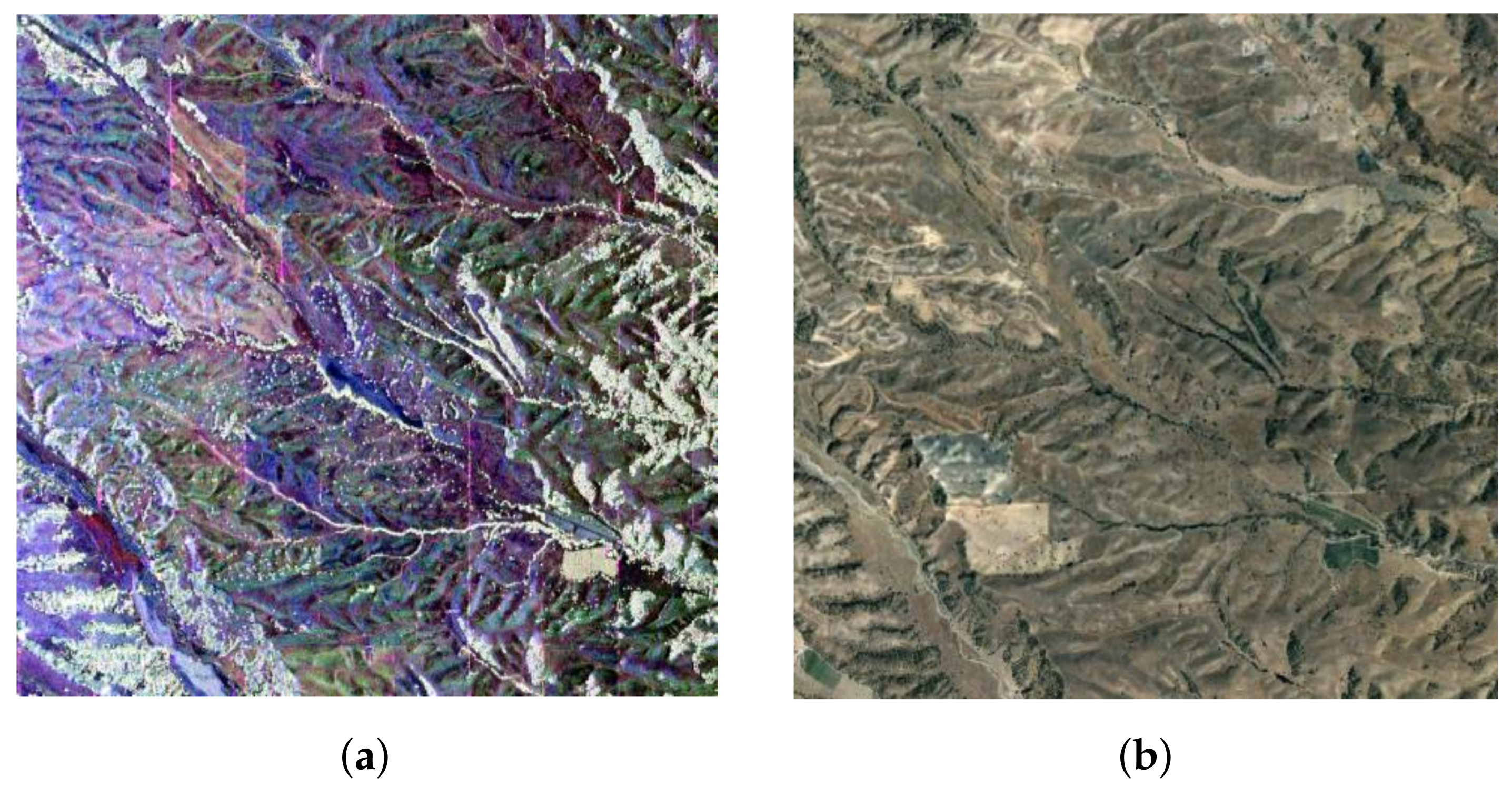
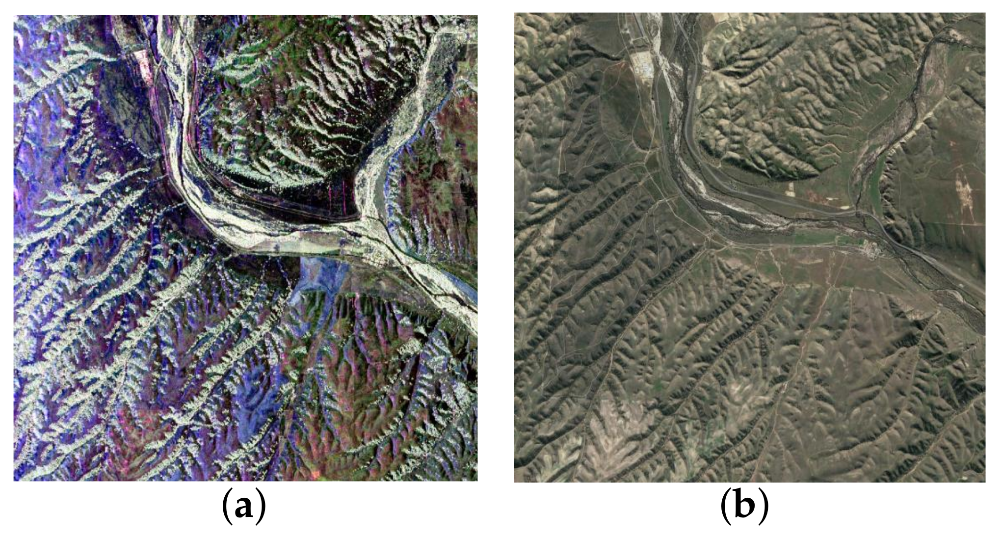
Figure 2.
(a) Pauli image of AIRSAR L-band data from Camp Roberts, 768 rows (azimuth) × 768 columns (ground range). (b) Corresponding area optical image from Google Earth. The direction of flight is from top to bottom.
Figure 2.
(a) Pauli image of AIRSAR L-band data from Camp Roberts, 768 rows (azimuth) × 768 columns (ground range). (b) Corresponding area optical image from Google Earth. The direction of flight is from top to bottom.
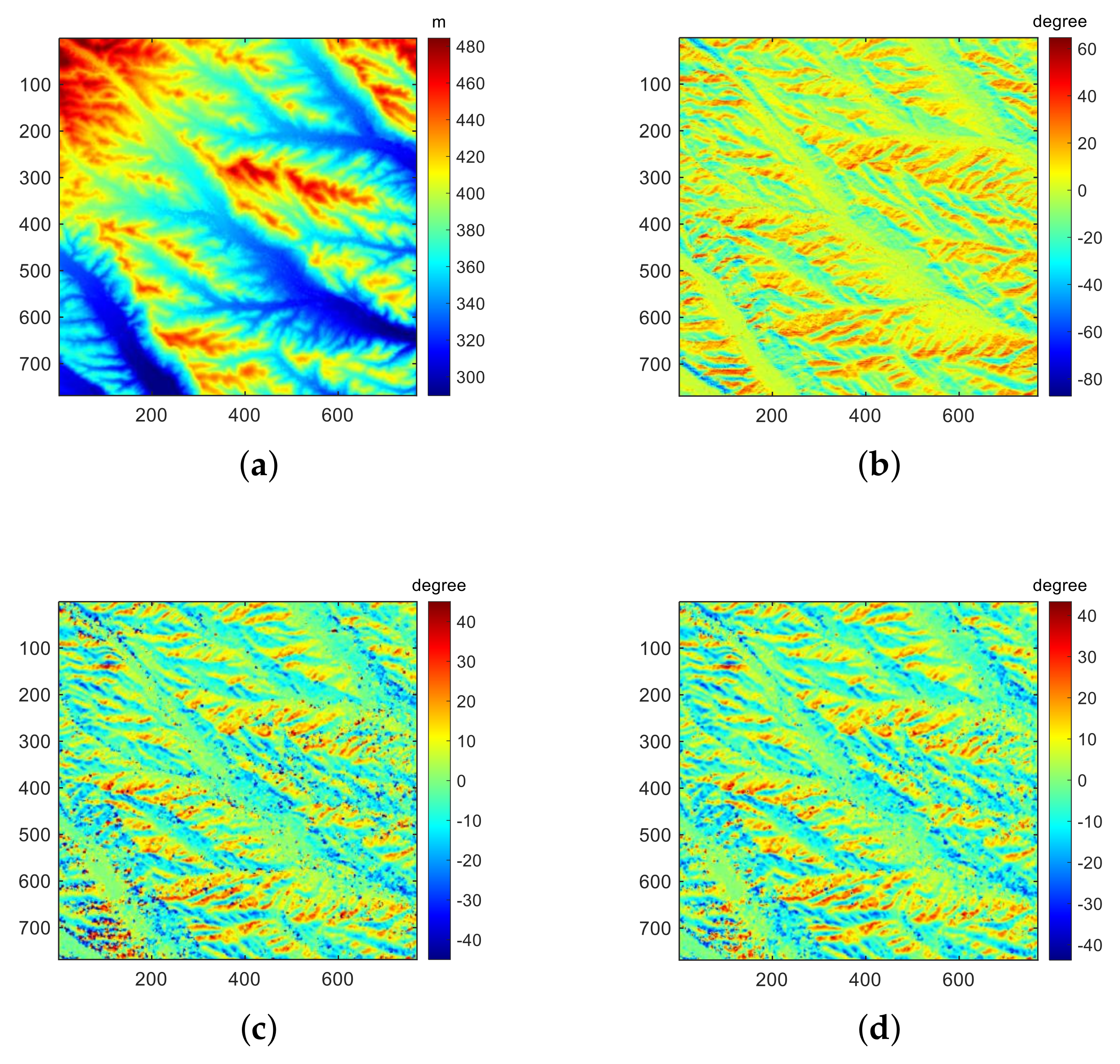
Figure 3.
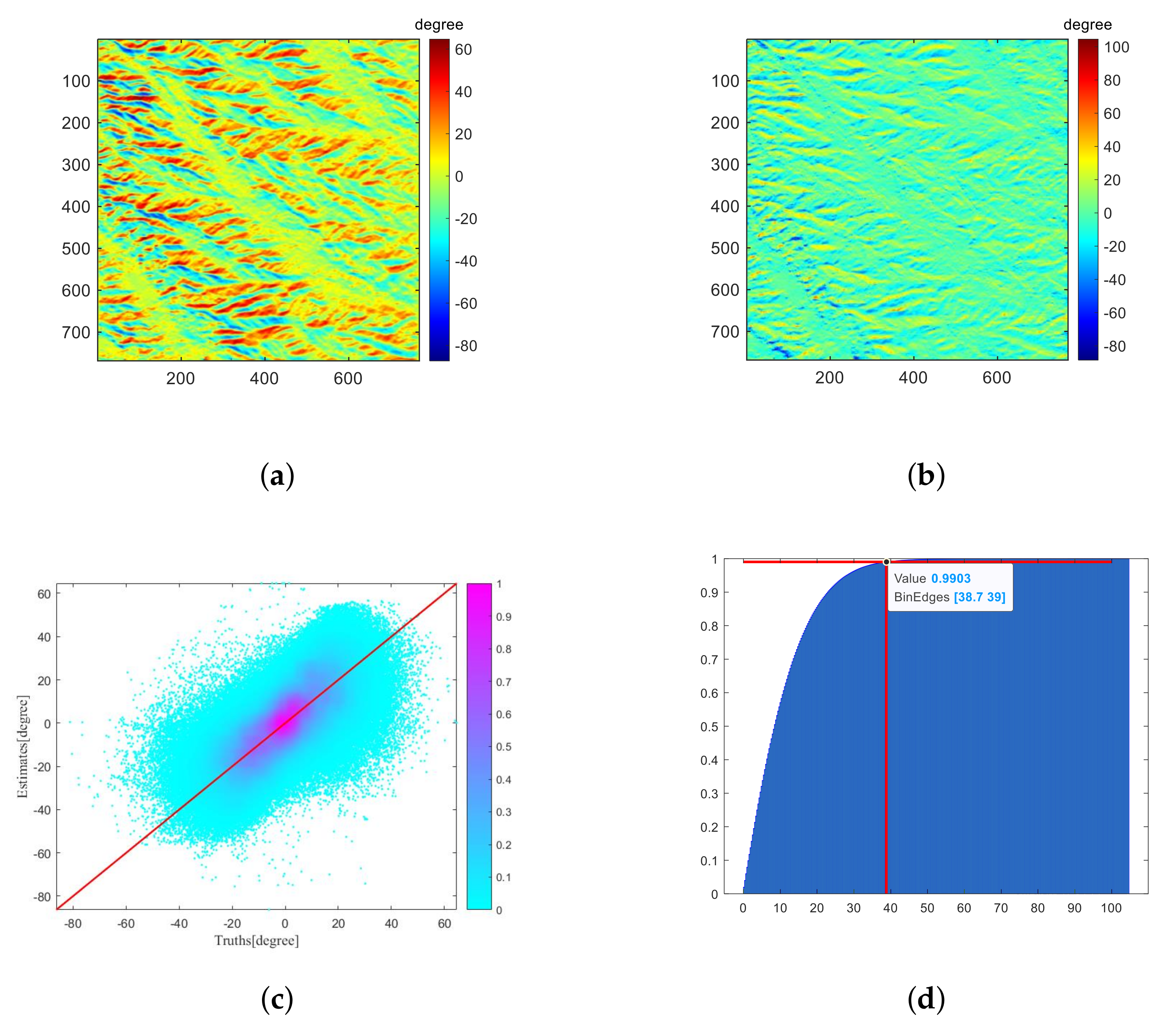
(a) C-band AIRSAR InSAR-generated DEM with approximately 10 m resolution. (b) POA from the DEM of (a). (c) POA from L-Band PolSAR data estimated by CPA. (d) POA from L-Band PolSAR data estimated by VEDA.
Figure 3.
(a) C-band AIRSAR InSAR-generated DEM with approximately 10 m resolution. (b) POA from the DEM of (a). (c) POA from L-Band PolSAR data estimated by CPA. (d) POA from L-Band PolSAR data estimated by VEDA.
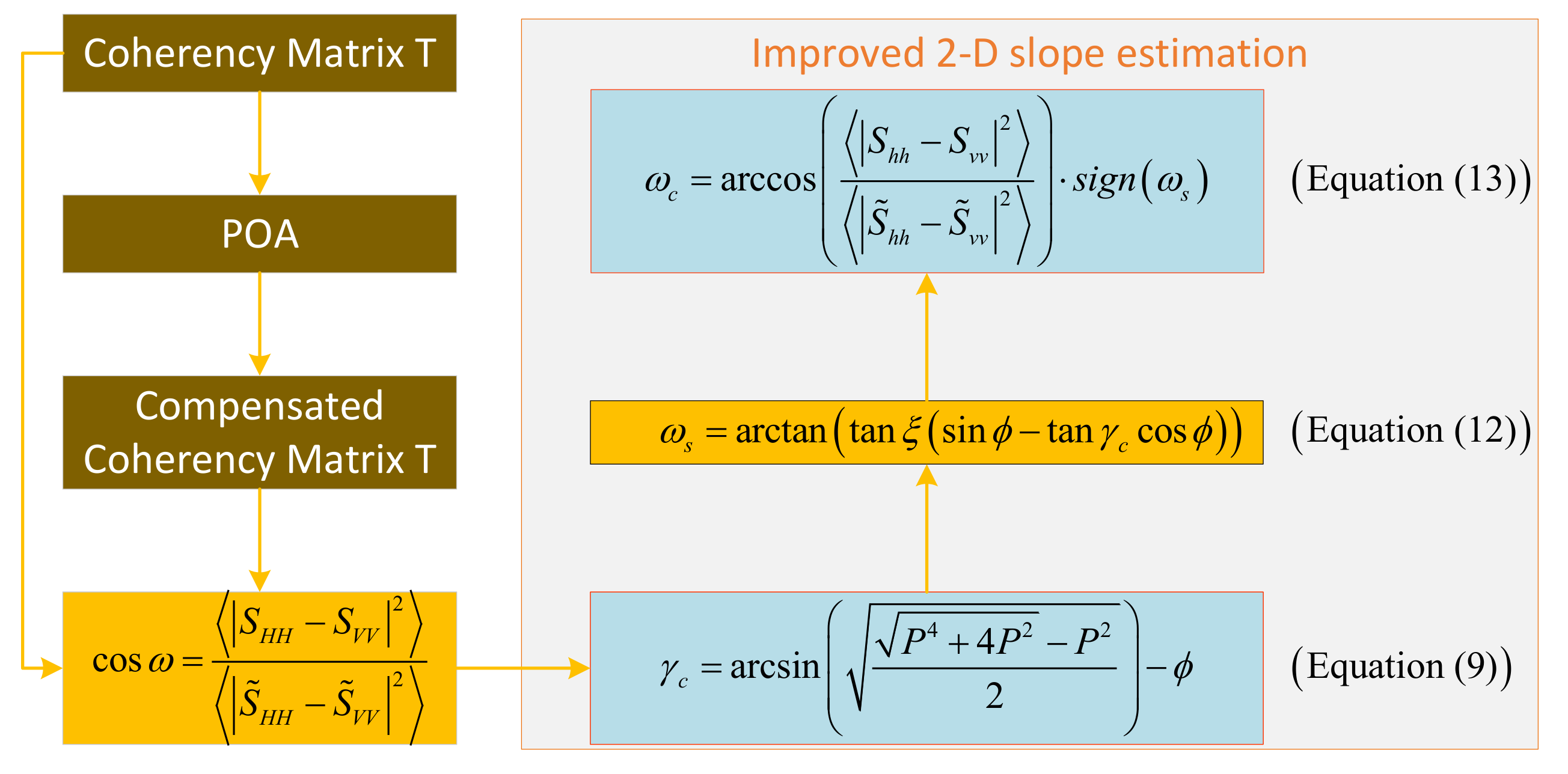
Figure 4.
The slope estimation flow chart proposed in this paper.
Figure 4.
The slope estimation flow chart proposed in this paper.
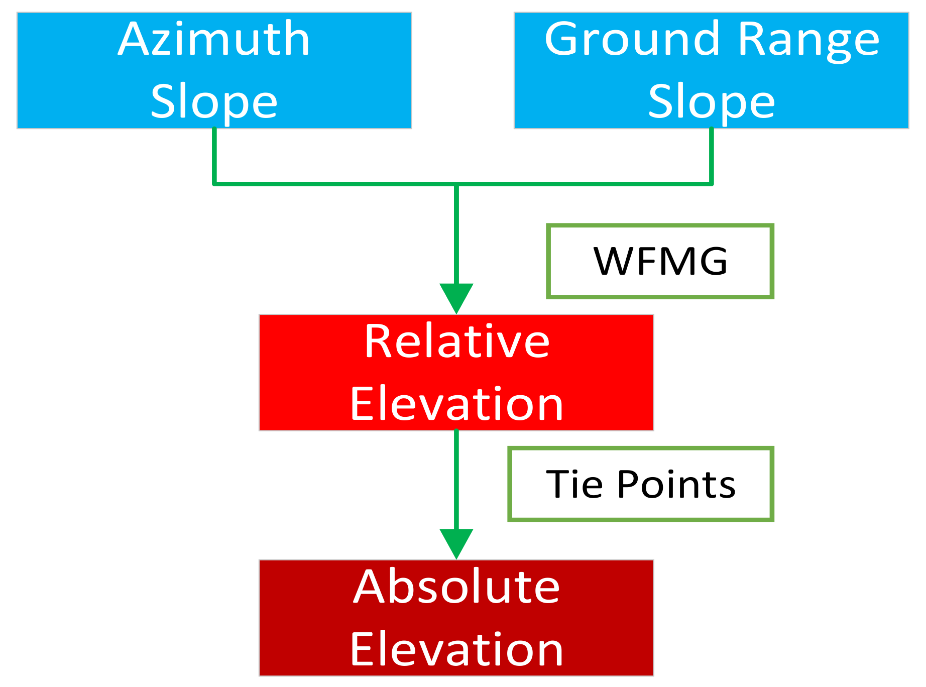
Figure 5.
Single-pass PolSAR topography retrieval processing diagram after the azimuth slope and the ground range slope are estimated.
Figure 5.
Single-pass PolSAR topography retrieval processing diagram after the azimuth slope and the ground range slope are estimated.
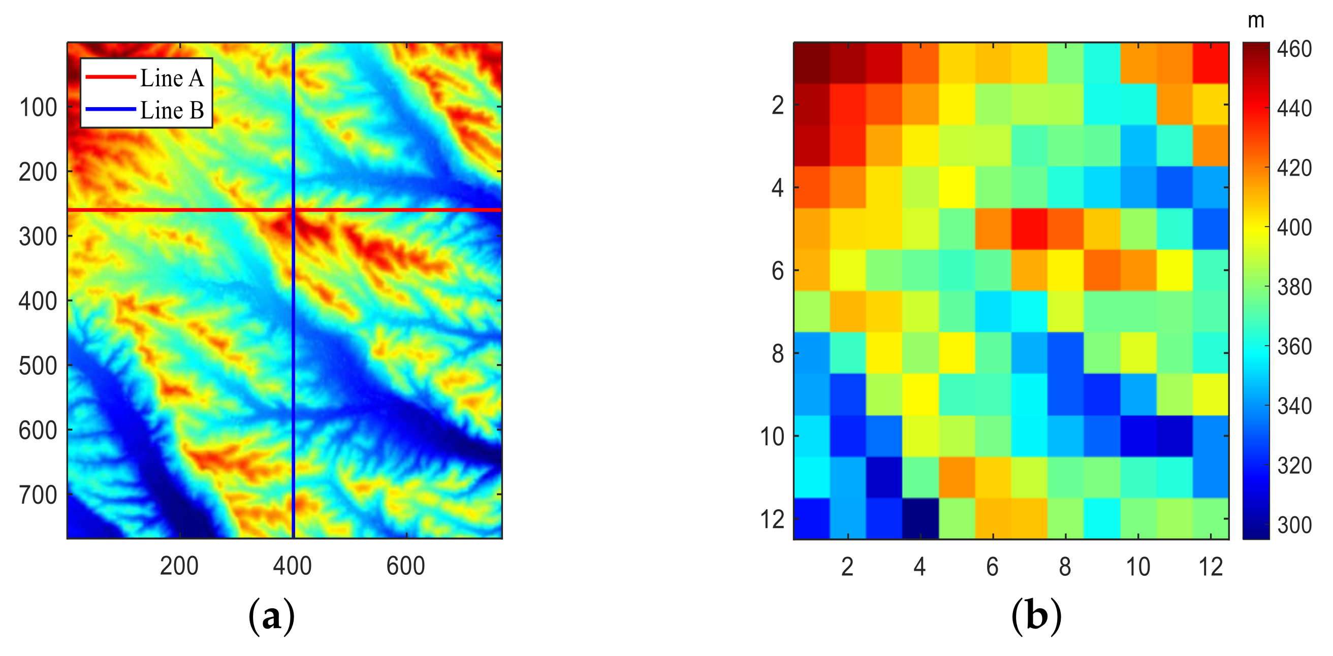
Figure 6.
Point matrix image. (a) C-band InSAR DEM. (b) Downsampled C-band InSAR DEM with approximately 640 m resolution as initial height.
Figure 6.
Point matrix image. (a) C-band InSAR DEM. (b) Downsampled C-band InSAR DEM with approximately 640 m resolution as initial height.
Figure 7.
DEM derived from L-band PolSAR data using the proposed method.
Figure 7.
DEM derived from L-band PolSAR data using the proposed method.
Figure 8.
(
a) Scatter plot between C-band AIRSAR InSAR-derived DEM (truths) and POLSAR derived DEM (estimates). (
b) The cumulative distribution function of elevation difference between
Figure 6a and
Figure 7. (
c) and (
d) are the comparison of DEM values measured along line A and line B in
Figure 6a.
Figure 9.
(a) RGB Pauli color-coded image with AIRSAR L-band data from Camp Roberts, 1024 rows (azimuth) × 1024 columns (ground range). (b) Corresponding area optical image from Google Earth. The direction of flight is from top to bottom.
Figure 9.
(a) RGB Pauli color-coded image with AIRSAR L-band data from Camp Roberts, 1024 rows (azimuth) × 1024 columns (ground range). (b) Corresponding area optical image from Google Earth. The direction of flight is from top to bottom.
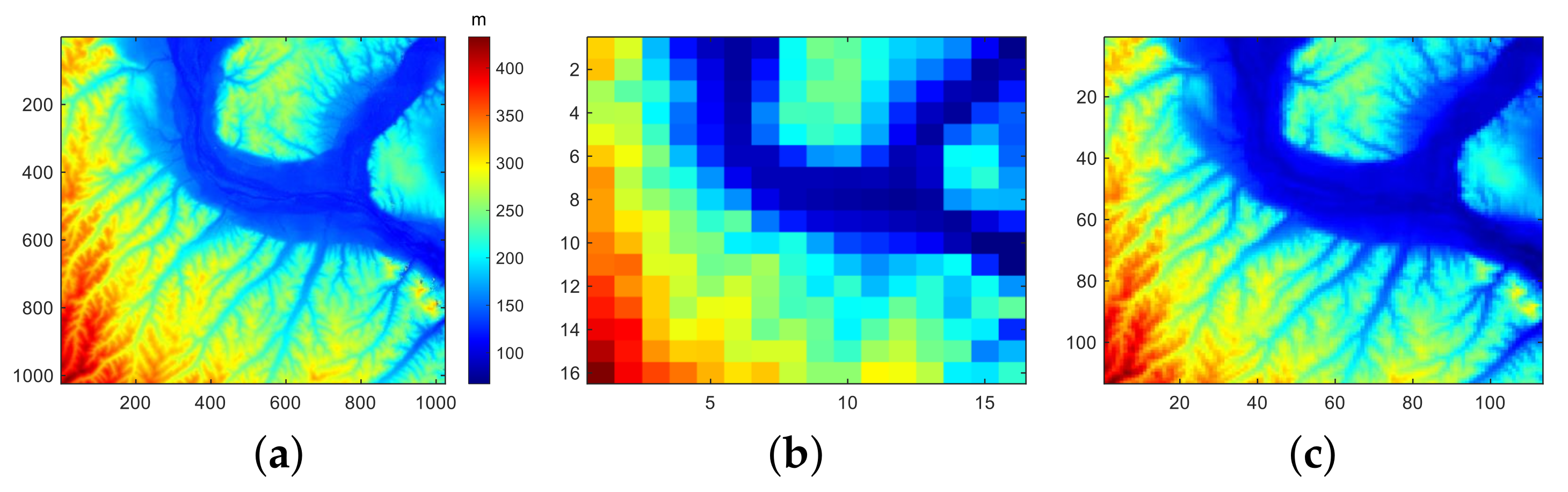
Figure 10.
(a) C-band AIRSAR InSAR generated DEM. Downsampled 640 m (b) and 90 m (c) resolution images.
Figure 10.
(a) C-band AIRSAR InSAR generated DEM. Downsampled 640 m (b) and 90 m (c) resolution images.
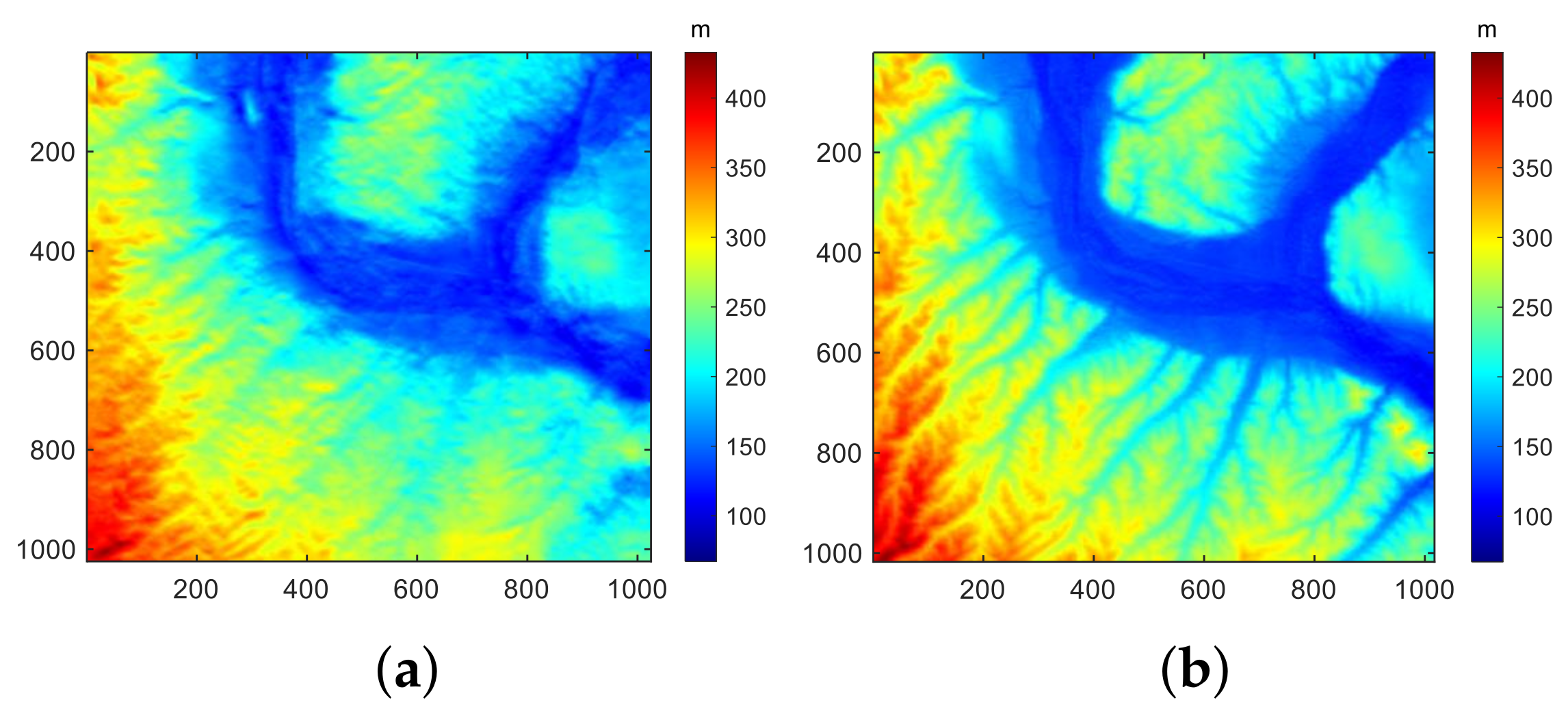
Figure 11.
DEM generated from L-band POLSAR data based on tie-points with resolutions of 640 m (a) and 90 m (b), respectively.
Figure 11.
DEM generated from L-band POLSAR data based on tie-points with resolutions of 640 m (a) and 90 m (b), respectively.
Figure 12.
Three regions of interest (ROI) are selected, as shown in (a); the tie-points are shown in (b–d) with a resolution of 90 m. (b–d) correspond to the red-, green-, and blue-marked areas in (a), respectively.
Figure 12.
Three regions of interest (ROI) are selected, as shown in (a); the tie-points are shown in (b–d) with a resolution of 90 m. (b–d) correspond to the red-, green-, and blue-marked areas in (a), respectively.
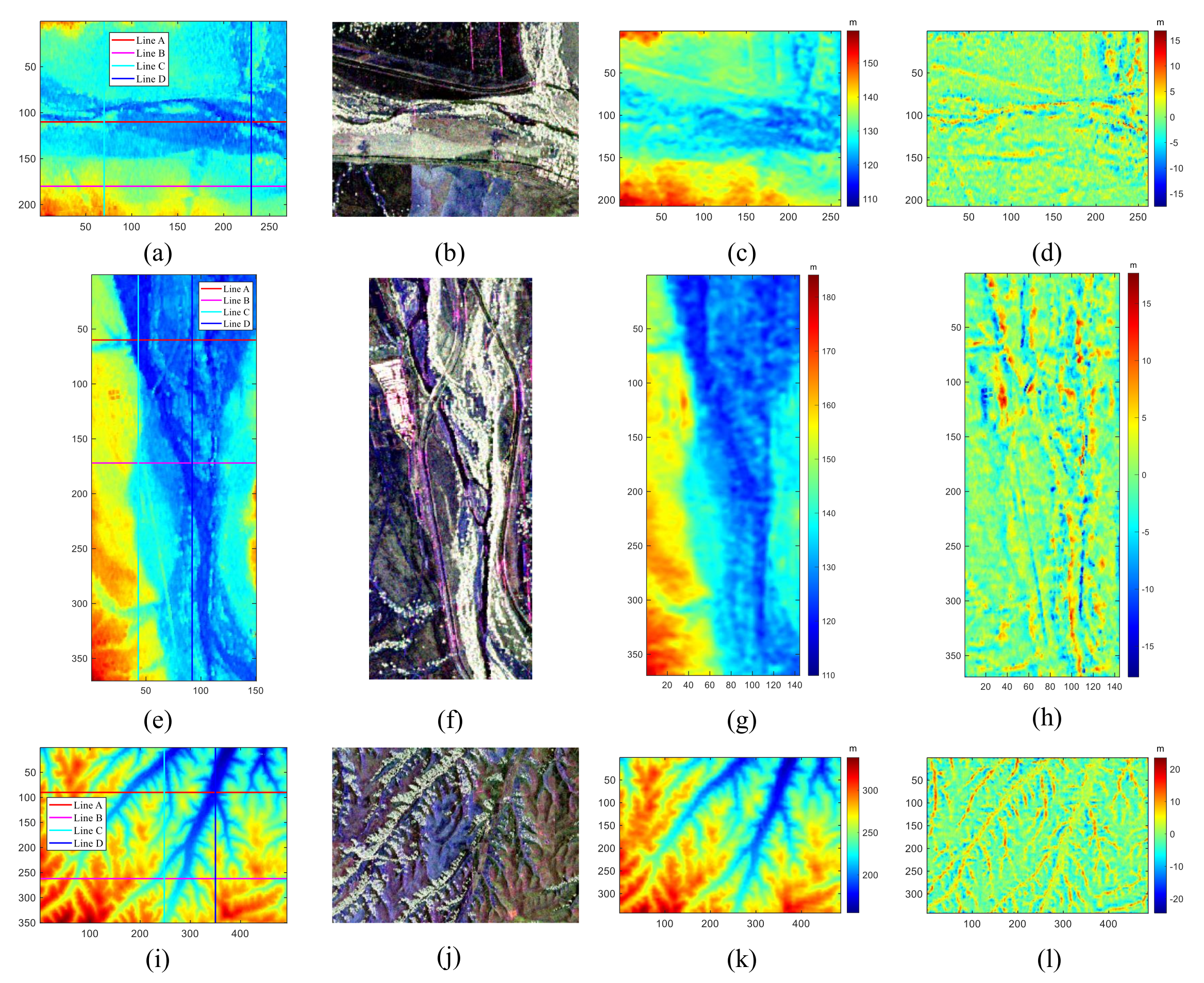
Figure 13.
The first and second columns are the corresponding C-band InSAR DEM and Pauli images, respectively, the third column is the DEM generated from PolSAR data and the fourth column is the difference image between the first and third columns. The first to third rows correspond to the red-, green-, and blue-marked areas in
Figure 12a, respectively. Further, combining the results of the first to third rows, it can be seen that the error of flat terrain is smaller, and the error is larger at the boundaries of different terrains.
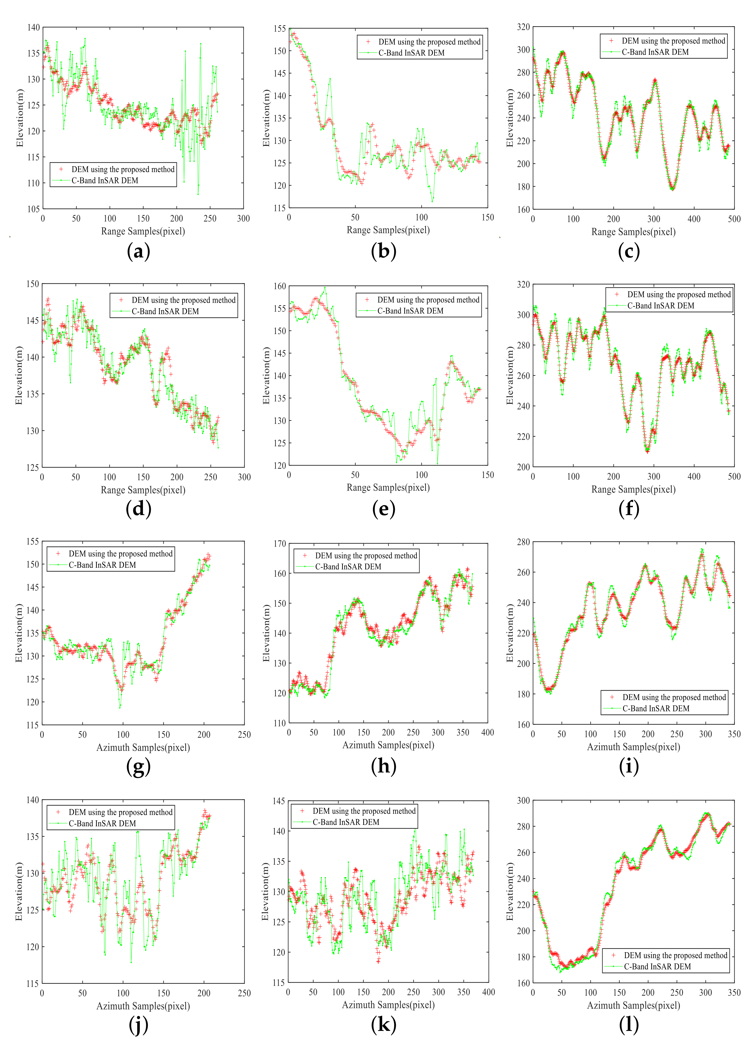
Figure 14.
The first to third columns correspond to
Figure 13a, e, and i, respectively, and the first to fourth rows correspond to the elevation profiles marked by lines A and D, respectively. It can be seen that the error depends on the terrain, and the error is larger where the elevation changes sharply. The more complex the terrain, the larger the error dynamic range.
Figure 15.
Point matrix image. (a) Downsampled C-band InSAR DEM to 90 m. (b) 30 m resolution as the initial height.
Figure 15.
Point matrix image. (a) Downsampled C-band InSAR DEM to 90 m. (b) 30 m resolution as the initial height.
Figure 16.
The first row is the DEM image derived from L-band PolSAR data and the second row is the scatter diagram between C-band InSAR DEM (truths) and PolSAR-derived DEM (estimates). Furthermore, the first and second columns correspond to the cases where the tie-points have 90 m and 30 m resolution, respectively. It can be seen that the higher the resolution of the tie-points, the closer the elevation estimate is to the ground truth.
Figure 17.
(
a) POA derived from PolSAR-derived DEM. (
b,
c) are the difference image and scatter plot between (
a) and
Figure 3a, respectively, with the POA derived from INSAR-derived DEM as the ground truth. (
d) is a cumulative distribution function plot of the absolute value of (
b).
Figure 17.
(
a) POA derived from PolSAR-derived DEM. (
b,
c) are the difference image and scatter plot between (
a) and
Figure 3a, respectively, with the POA derived from INSAR-derived DEM as the ground truth. (
d) is a cumulative distribution function plot of the absolute value of (
b).
Figure 18.
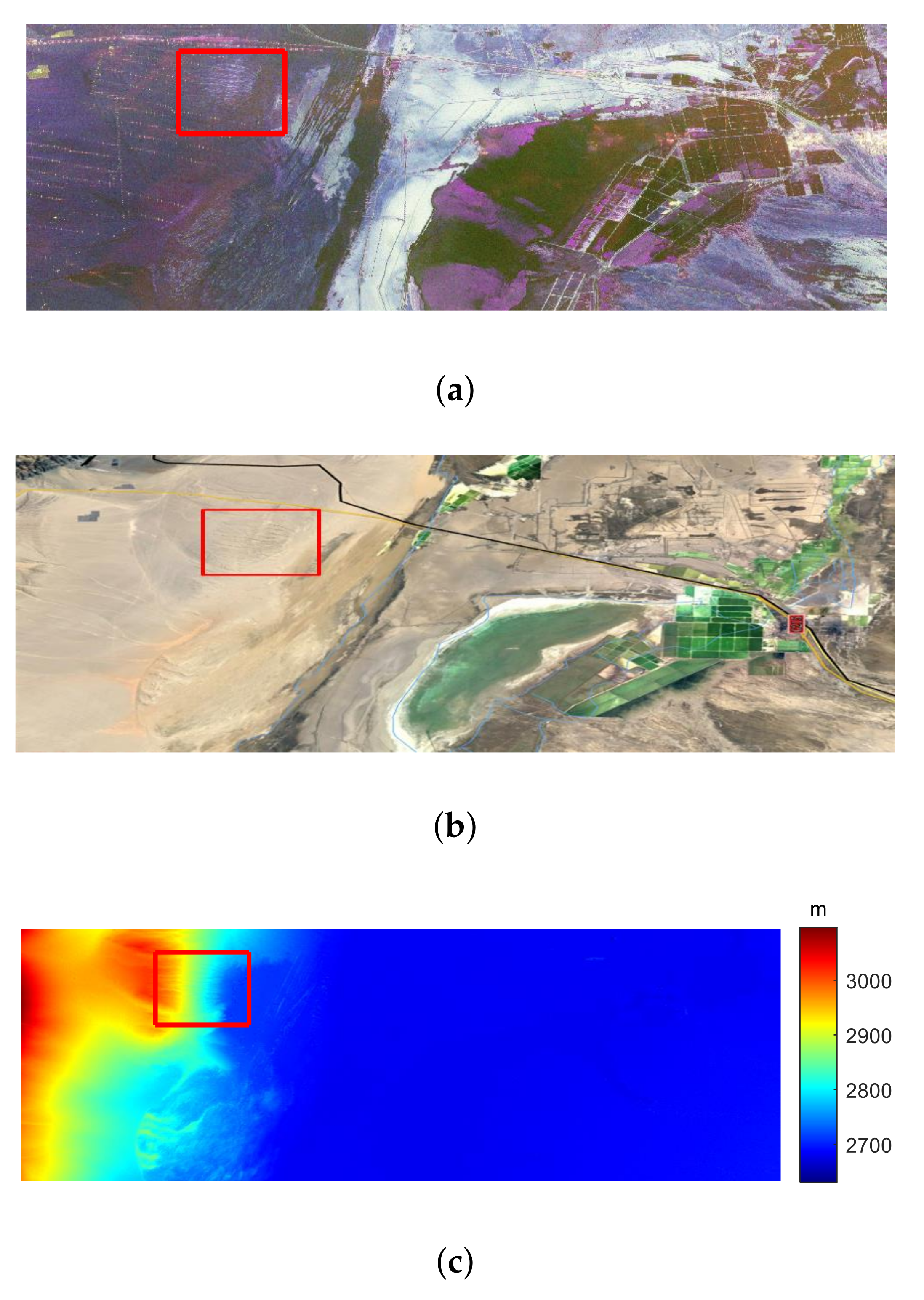
(a) RGB Pauli color-coded image with ALOS-2 PALSAR2 L-band data from Qinghai Salt Lake, 25,960 columns (azimuth) × 8624 rows (slant range). (b) Corresponding area optical image from Google Earth. (c) DEM data acquired by the Shuttle Radar Topography Mission (SRTM) at a resolution of 1 arc-second (30 m) in the corresponding area. The area marked by the red box is the region of interest.
Figure 18.
(a) RGB Pauli color-coded image with ALOS-2 PALSAR2 L-band data from Qinghai Salt Lake, 25,960 columns (azimuth) × 8624 rows (slant range). (b) Corresponding area optical image from Google Earth. (c) DEM data acquired by the Shuttle Radar Topography Mission (SRTM) at a resolution of 1 arc-second (30 m) in the corresponding area. The area marked by the red box is the region of interest.
Figure 19.
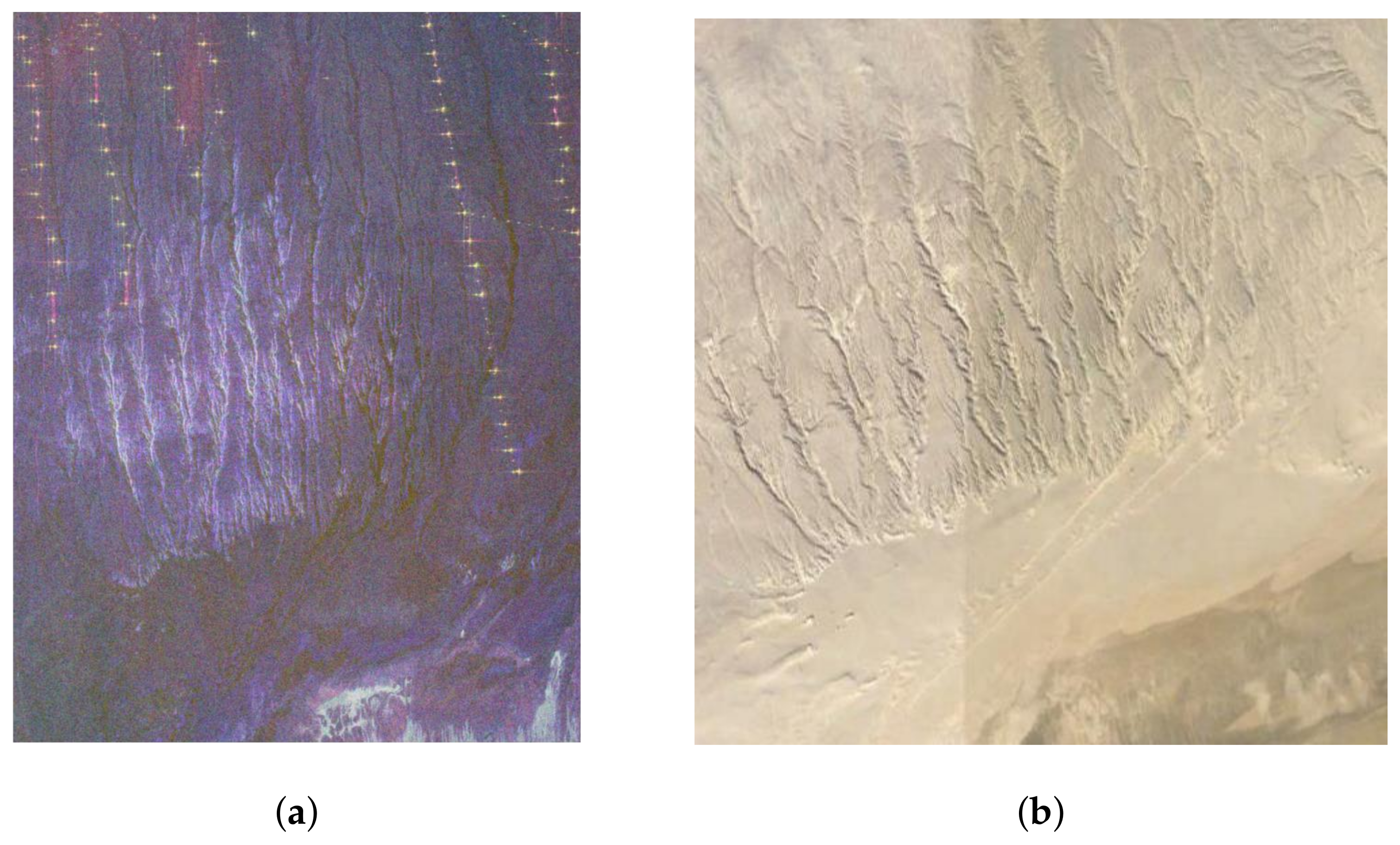
The region of interest selected in the experiment. (
a) corresponds to the boxed area in
Figure 18a, 3200 rows (azimuth) × 2486 columns (slant range). (
b) Corresponding area optical image from Google Earth.
Figure 19.
The region of interest selected in the experiment. (
a) corresponds to the boxed area in
Figure 18a, 3200 rows (azimuth) × 2486 columns (slant range). (
b) Corresponding area optical image from Google Earth.
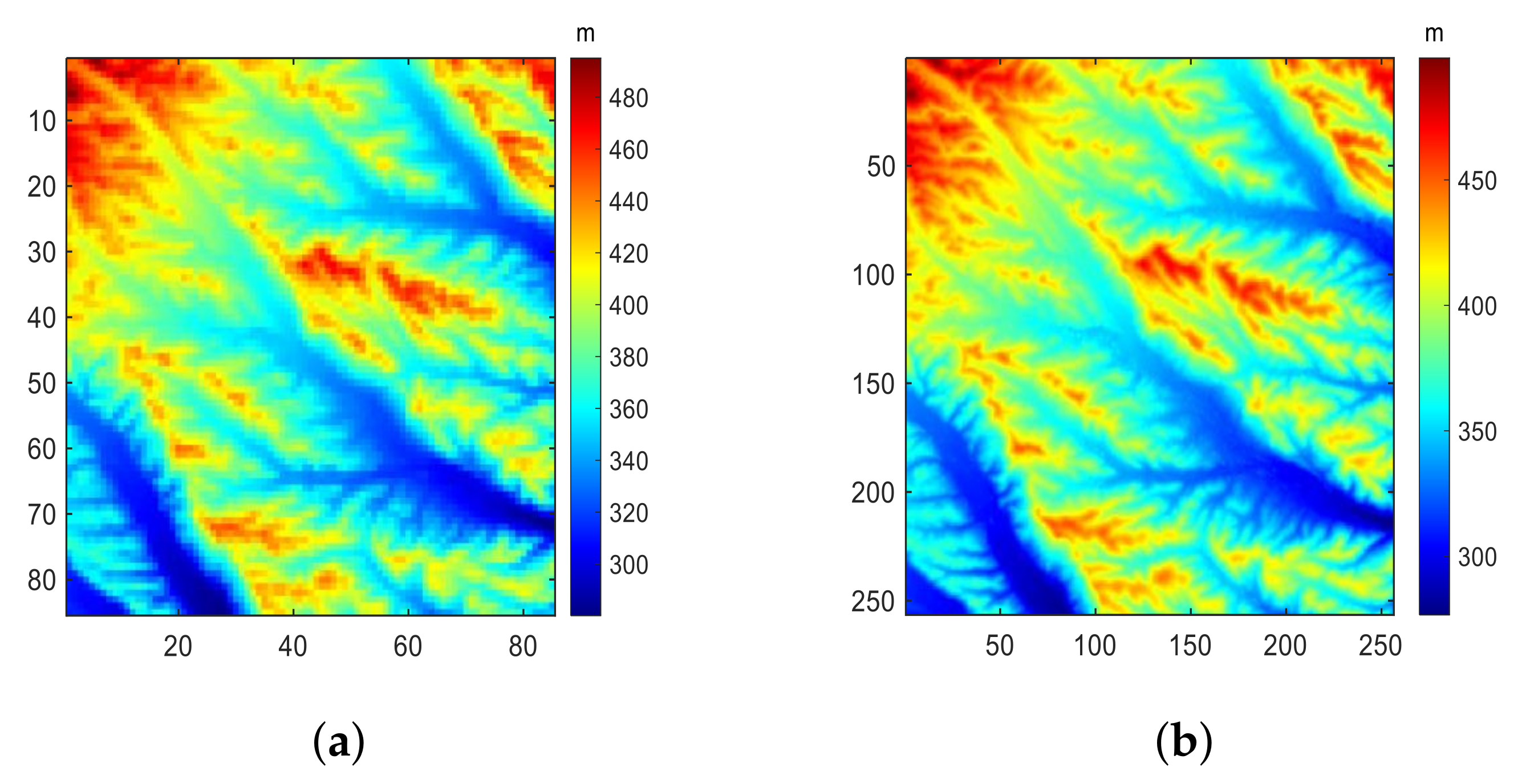
Figure 20.
(a) DEM from SRTM. Downsampled 90 m (b) and 30 m (c) resolution images.
Figure 20.
(a) DEM from SRTM. Downsampled 90 m (b) and 30 m (c) resolution images.
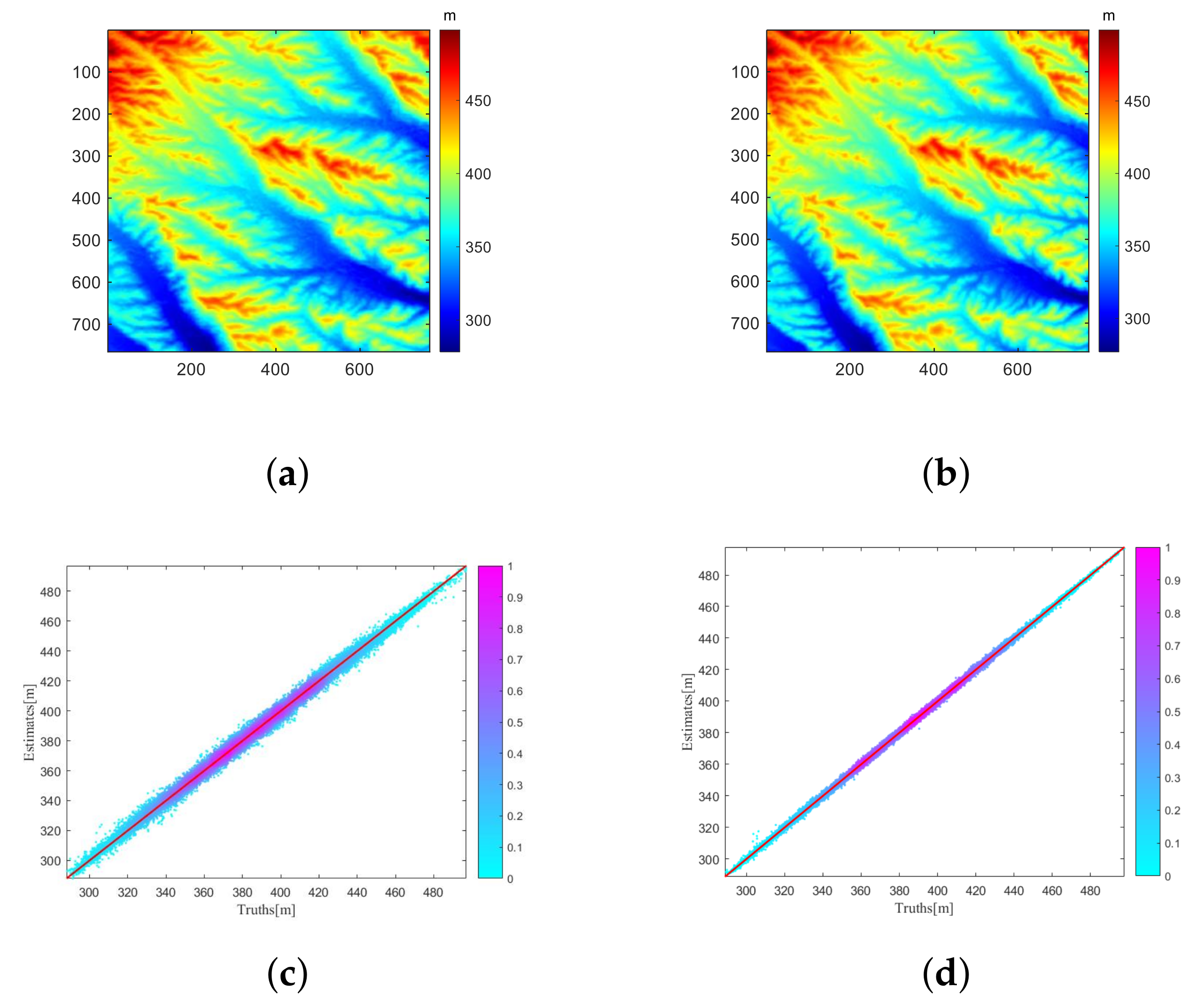
Figure 21.
The first row is the DEM image derived from L-band PolSAR data and the second row is the scatter diagram between SRTM DEM (truths) and PolSAR-derived DEM (estimates). The first and second columns correspond to the cases where the tie-points have 90 m and 30 m resolution, respectively. It can be seen that the higher the resolution of the tie-points, the closer the elevation estimate is to the ground truth.
Table 1.
RMSD of the POA estimates and ground truth results.
Table 1.
RMSD of the POA estimates and ground truth results.
| | CPA | VEDA |
|---|
| RMSD (°) | 11.24 | 10.10 |
Table 2.
RMSD of slope estimates and ground truth results (degrees).
Table 2.
RMSD of slope estimates and ground truth results (degrees).
| | Azimuth Slope | Ground Range Slope |
|---|
| Chen’s method | 9.87 | 9.77 |
| Li’s method | 5.03 | 6.26 |
| Proposed method | 3.50 | 6.04 |
Table 3.
RMSD of the height estimates and ground truth results.
Table 3.
RMSD of the height estimates and ground truth results.
| | Chen’s Method | Li’s Method | Proposed Method |
|---|
| RMSD (m) | 28.66 | 14.75 | 10.87 |
Table 4.
RMSD of the height estimates and ground truth results.
Table 4.
RMSD of the height estimates and ground truth results.
| Tie Points Res. | 640 (m) | 90 (m) |
|---|
| RMSD (m) | 13.00 | 2.30 |
Table 5.
RMSD of slope estimates and ground truth results (degrees).
Table 5.
RMSD of slope estimates and ground truth results (degrees).
| Tie Points Res. | Azimuth Slope | Ground Range Slope |
|---|
| 640 (m) | 4.82 | 5.75 |
| 90 (m) | 1.63 | 2.00 |
Table 6.
RMSD of the height estimates and ground truth results.
Table 6.
RMSD of the height estimates and ground truth results.
| Data | ROI1 | ROI2 | ROI3 |
|---|
| RMSD (m) | 1.04 | 1.64 | 2.40 |
Table 7.
RMSD of slope estimates and ground truth results (degrees).
Table 7.
RMSD of slope estimates and ground truth results (degrees).
| Data | Azimuth Slope | Ground Range Slope |
|---|
| ROI1 | 1.09 | 0.89 |
| ROI2 | 0.97 | 1.60 |
| ROI3 | 1.56 | 2.10 |
Table 8.
RMSD of the height estimates and ground truth results.
Table 8.
RMSD of the height estimates and ground truth results.
| Tie Points Res. | 90 (m) | 30 (m) |
|---|
| RMSD (m) | 3.20 | 1.14 |
Table 9.
RMSD of slope estimates and ground truth results (degrees).
Table 9.
RMSD of slope estimates and ground truth results (degrees).
| Tie Points Res. | Azimuth Slope | Ground Range Slope |
|---|
| 90 (m) | 3.10 | 2.33 |
| 30 (m) | 0.83 | 0.75 |
Table 10.
RMSD of the height estimates and ground truth results.
Table 10.
RMSD of the height estimates and ground truth results.
| Tie Points Res. | 90 (m) | 30 (m) |
|---|
| RMSD (m) | 2.23 | 0.92 |
Table 11.
RMSD of slope estimates and ground truth results (degrees).
Table 11.
RMSD of slope estimates and ground truth results (degrees).
| Tie Points Res. | Azimuth Slope | Ground Range Slope |
|---|
| 90 (m) | 3.32 | 5.03 |
| 30 (m) | 1.54 | 3.08 |


