Article

Spatiotemporal Characteristics and Heterogeneity of Vegetation Phenology in the Yangtze River Delta

1
State Forestry and Grassland Administration Key Laboratory of Forest Resources & Environmental Management, Beijing Forestry University, Beijing 100083, China
2
Anhui Province Key Laboratory of Physical Geographic Environment, Chuzhou University, Chuzhou 239000, China
3
Institute of Water Resources and Hydro-Electric Engineering, Xi’an University of Technology, Xi’an 710048, China
4
Shaanxi Provincial Land Engineering Construction Group Co., Ltd., Xi’an 710075, China
5
Intelligent Forestry Key Laboratory of Haikou City, College of Forestry, Hainan University, Haikou 570228, China
*
Author to whom correspondence should be addressed.
Remote Sens. 2022, 14(13), 2984; https://doi.org/10.3390/rs14132984
Submission received: 10 May 2022 / Revised: 13 June 2022 / Accepted: 20 June 2022 / Published: 22 June 2022
(This article belongs to the Special Issue Remote Sensing of Greenhouse Gas Emissions)

Abstract

:
Vegetation phenology and its spatiotemporal driving factors are essential to reflect global climate change, the surface carbon cycle and regional ecology, and further quantitative studies on spatiotemporal heterogeneity and its two-way driving are needed. Based on MODIS phenology, meteorology, land cover and other data from 2001 to 2019, this paper analyzes the phenology change characteristics of the Yangtze River Delta from three dimensions: time, plane space and elevation. Then, the spatiotemporal heterogeneity of phenology and its driving factors are explored with random forest and geographic detector methods. The results show that (1) the advance of start of season (SOS) is insignificant—with 0.17 days per year; the end of season (EOS) shows a significant delay—0.48 days per year. The preseason temperature has a greater contribution to SOS, while preseason precipitation is main factor in determining EOS. (2) Spatial differences of the phenological index do not strictly obey the change rules of latitude at a provincial scale. The SOS of Jiangsu and Anhui is earlier than that of Zhejiang and Shanghai, and EOS shows an obvious double-clustering phenomenon. In addition, a divergent response of EOS with elevation grades is found; the most significant changes are observed at grades below 100 m. (3) Land cover (LC) type is a major factor of the spatial heterogeneity of phenology, and its change may also be one of the insignificant factors driving the interannual change of phenology. Furthermore, nighttime land surface temperature (NLST) has a relatively larger contribution to the spatial heterogeneity in non-core urban areas, but population density (PD) contributes little. These findings could provide a new perspective on phenology and its complex interactions between natural or anthropogenic factors.

1. Introduction

Vegetation phenology refers to the changes in plant characteristics caused by natural environment and climate change, such as germination, flowering, fruiting and defoliation [1,2]. Vegetation phenology affects the surface carbon cycle, terrestrial ecosystem and energy exchange [3,4,5,6] and is closely related to agricultural production and environmental ecology [4,7,8]. As one of the important indicators that can reflect the dynamic change of vegetation and climate change [9,10], the research on the temporal and spatial pattern of vegetation phenology and its related factors has attracted more and more attention.
Many scholars have analyzed the spatiotemporal characteristics of regional phenology and concluded that spring phenology is advanced and that autumn phenology is delayed [4,9,11]. Meanwhile, other studies have found a different conclusion in eastern China and Nanjing due to the complexity of the influencing factors [4,12,13]. Methods such as statistical analysis, correlation, and random forests were used to explore the temporal variation characteristics of phenology and response mechanisms [11,14,15,16,17,18]. In terms of space, the study concluded that spring and autumn phenology in different regions are different with spatial heterogeneity [11,12,14,19]. Although these studies involved the spatial analysis and the conclusion of heterogeneity, little quantitative analysis and discussion of driving factors of heterogeneity has been shown. Some scholars have proposed that the phenological characteristics of different vegetation cover types are different [15,20] and that changes in vegetation cover types will lead to changes in phenology [17,21,22], but quantitative evaluation still requires further research.
Among the influencing factors, temperature and precipitation have become the main climate factors explaining the interannual variation of phenology. Many studies have shown that there is a significant negative or positive correlation between start or end of vegetation growth season (SOS or EOS) and temperature or precipitation [9,11]. At the same time, the impact of climatic conditions on vegetation phenology has an obvious lag effect [9,23,24]. Piao [9] pointed out that in the temperate zone of China, the increase in average temperature in spring leads to the advancement of SOS, and the increase of the average temperature in autumn leads to the delay of EOS. There is a significant negative correlation between SOS and average temperature in the 2–3 months before the season [9,11,25]. Relevant scholars have found that feedback between temperature, precipitation and vegetation phenology is at its greatest in the first month preseason [14,26] and directly use the climate factors in first month preseason to conduct phenological related research and obtain better results [11]. Precipitation has an obvious regulatory effect on phenology in areas that are sensitive to precipitation [8,27]. Research on grasslands in arid and semiarid regions of northeast China [28] and desert grasslands in Inner Mongolia [23] concluded the greening period is mainly controlled by preseason precipitation, SOS in Qinghai is mainly affected by precipitation, and EOS is mainly affected by precipitation and temperature simultaneously [11]. Moreover, studies have shown that diurnal temperature difference has a significant impact on phenology. For example, increased temperature during the day will lead to higher evaporation and lower water content in the root zone [29], thereby inhibiting vegetation growth. Under nocturnal warming, the carbon uptake by plants through leaf photosynthesis overcompensates for the respiration carbon release caused by increased temperature, which promotes plants to accumulate more carbon [30] and may lead to earlier flowering. Meanwhile, Meng [31] and Piao [32] believe that daytime temperature has a higher impact on phenology than nighttime.
In addition, photoperiod has gradually been paid more attention to, and the hypothesis of “photoperiod limitation” has been proposed [33,34,35]. Studies have shown that photoperiod, and its interaction with temperature and other factors, can affect phenology [36,37,38]. The viewpoint of “warmer winter temperatures reduce the sensitivity of phenology to temperature, thus slowing down the advance of spring phenology” was put forward [34]. Photoperiod can also regulate spring phenology by advancing late leaf-out caused by temperature variations [39]. However, Zohner [40] pointed out that “species from high latitudes with long winters leafed out independent of photoperiod”, which makes phenological prediction more complicated. Additionally, the phenology of different tree species responds differently to photoperiod [33,38,39,40], which will become one of the important factors for the change of forest ecological structure under climate warming.
Beyond that, altitude [11,41,42,43], latitude and longitude [19] and urbanization or human activities [4,44] have also become factors affecting phenology. In particular, research on the impact of urbanization on phenology has become a hotspot. Meng [45] pointed out that urban warming advances spring phenology but reduces the response of phenology to temperature in United States. Related research shows that the phenology shifted earlier for SOS, later for EOS, and lengthened for the growing season length (GSL) in urban core areas (urbanization intensity above 50%) relative to their rural counterparts [16,19]. From the heterogeneity of land surface temperature (LST) within the city, the phenological response to it was studied by Samuel C Zipper et al. [46], and it was concluded that the urban phenology is affected by the local surface cover and microclimate, the urban-rural transition zone and local lakes affects GSL.
The above studies have deepened the understanding of the impact mechanism of phenology and provided a basis for the analysis and application of regional and local phenological characteristics. Studies have shown that the sensitivity of spring phenology to temperature in Europe decreases with an increase in temperature [34], while precipitation is more sensitive to arid and semiarid regions [23,27]. It can be seen that vegetation phenology in different geographical locations responds differently to climatic factors, and the influencing factors are also different in regions with different geographical environments, such as mountains, plains, urban and rural areas. Quantitative research on the characteristics of regional phenology and its impact mechanisms is of great significance to the study of climate change and sustainable development. As one of the key urban agglomerations in China, the Yangtze River Delta is affected by both the natural environment and human activities. Studies on its phenology include urban–rural differences, parameter extraction and spatiotemporal changes [16,47,48,49], but the responses and driving factors of its spatiotemporal heterogeneity have not been explained in detail.
In order to provide a better understanding of regional environmental change and land use management, this paper quantitatively analyzes its spatiotemporal heterogeneity and driving factors by introducing random forest and geographic detector methods based on the analysis of the variation characteristics of vegetation phenology. At the same time, we will answer two questions based on the geographical background and its intense human activity: Firstly, what are the characteristics of phenological spatiotemporal changes in the Yangtze River Delta; are they consistent with the rules of latitude change in previous studies? Secondly, what drives the spatiotemporal changes of vegetation phenology in the Yangtze River Delta?

2. Materials and Methods

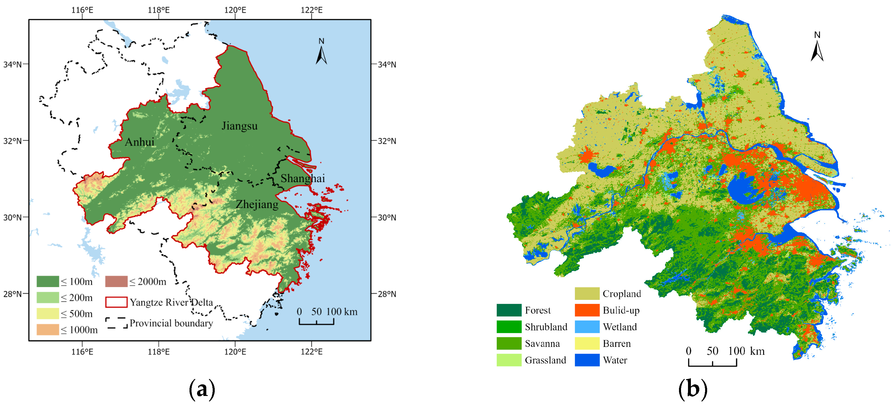
2.1. Experimental Area

The Yangtze River Delta urban agglomeration (Yangtze River Delta for short) is located in the lower reaches of the Yangtze River in China (Figure 1a). It is close to the Yellow Sea and the East China Sea. According to the “Yangtze River Delta Urban Agglomeration Development Plan (2014–2020)”, the Yangtze River Delta is within the scope of Shanghai, Jiangsu Province, Zhejiang Province and Anhui Province [16,50]. The Yangtze River Delta has a subtropical monsoon climate, crisscrossing rivers and lakes, dense population, numerous cities and great human interference (Figure 1b). Meanwhile, Dabie Mountain in western Anhui—the mountain region in southern Anhui—and in western and southern Zhejiang are the key areas that constitute the green ecological barrier.

2.2. Data and Preprocessing

The experimental data in this paper include the vegetation phenological (VP) data, land cover (LC) data, meteorological data (MD), population density (PD) data, digital elevation model (DEM) and land surface temperature (LST) of the Yangtze River Delta from 2001 to 2019. All data processing was carried out in the Google Earth Engine platform (GEE). The VP data in this paper are Moderate Resolution Imaging Spectrometer (MODIS) Global Vegetation Phenology product (MCD12Q2), which were accessed at https://lpdaac.usgs.gov/ (accessed on 25 November 2021) with a resolution of 500 m.
Referring to previous studies [53], the MCD12Q1 V6 products were used in the paper to determine LC, which provides global land cover types at yearly intervals (Figure 1b). The data were derived using supervised classifications of MODIS Terra and Aqua reflectance data. The resolution was 500 m and used the Annual International Geosphere-Biosphere Programme (IGBP) classification types. Combined with the characteristics of the study area, the paper classified the terrain into forest, shrubland, savanna, grassland, cropland and build-up areas. The area of shrubland in the study area was relatively small (as can be seen in Section 4.2 below), so no separate analysis was made in this paper.
Temperatures at 2 m and total precipitation data were extracted from the ECMWF atmospheric reanalysis data [17] (https://www.ecmwf.int/en/publications (accessed on 10 December 2021)) and resampled to 500 m resolution. The PD dataset is available to download at a resolution of 30 arc seconds (approximately equal to 1 km at the equator) (https://www.worldpop.org/ (accessed on 15 February 2022)). The units are the number of people per square kilometer based on country totals adjusted to match the corresponding official United Nations population estimates that have been prepared by the Population Division of the Department of Economic and Social Affairs of United Nations Secretariat. SRTM DEM come from https://cmr.earthdata.nasa.gov/ (accessed on 17 March 2022). In order to further explore the differences in the effect of different altitudes on phenology, the altitudes were divided into 0–100 m, 100–200 m, 200–500 m, 500–1000 m, 1000–1500 m and 1500–2000 m to be combined with the geographical conditions of the study area and references [54].

2.3. Extraction of Vegetation Phenology Information

MCD12Q2 Version 6 data product was derived from time series of the two-band enhanced vegetation index (EVI2) calculated from MODIS Nadir Bidirectional Reflectance Distribution Function (BRDF)-adjusted reflectance (NBAR). Greenup was defined as the date when EVI2 first exceeded 15% of the segment’s EVI2 amplitude, and dormancy was defined as the date when EVI2 last exceeded 15% of the segment’s EVI2 amplitude. This article took greenup and dormancy as SOS and EOS from MCD12Q2 data. For pixels with more than two valid vegetation cycles, the data represent the two cycles with the largest NBAR-EVI2 amplitudes. SOS in this article adopted the value of the earliest cycle, while EOS was the maximum value between dormancy1 and dormancy2. From dormancy2, it can be seen that the crop rotation period is obvious, and there is a very small amount of forest and built-up vegetation in the study area. In order to facilitate statistical research, the paper converted each value of the phenological index (Days since 1 January 1970) to the day of current year (DOY). The quality of the MODIS phenology product has a good agreement with field observations [4,15,55,56]. Poor quality data were excluded according to the quality analysis layer, and pixels with SOS values before DOY 0 or later than DOY 180 were removed from the analysis [4,57]. The indicator of GSL is also included in this paper, which was defined as the length between the SOS and EOS.

2.4. Analysis of Phenological Changes

In terms of the temporal variation characteristic of phenology, on one hand, least squares linear regression was used to analyze the changing trend of vegetation phenology from 2001 to 2019 [11,15,57], and a nonparametric significance test—the Mann–Kendall (MK) test [58]—was used to detect the significance of trends. The slope of the trend line of the multiyear regression equation represents the interannual change rate, and p value was used to illustrate its significance. If the slope is positive, it means that the phenology is delayed. Otherwise, the vegetation phenology is advanced. On the other hand, in order to explore the relationship between phenology, climate, population density and other factors, this paper selected partial correlation analysis [42] and Pearson correlation coefficient to study its correlation and conduct a significance test.

2.5. Spatiotemporal Heterogeneity Analysis

Random forest is a decision tree algorithm [59] which has been applied to identify the response mechanisms of vegetation phenology [11,17,18]. According to the concentration of phenological index values in the experimental area, one month before the start and end of phenology were selected (i.e., January, February, March, and September, October, November), and two months were extended before as reference (i.e., November, December for SOS and July, August for EOS). The period including these months was defined as preseason. In this paper, the index of increase in node purity (IncNodePurity) of the random forest was selected to rank the importance of factors. In order to express the relative importance more conveniently, the paper adjusted the results and expressed them with the proportion of importance (%). That is, the index value of each factor was divided by the sum of the index value of all factors. Furthermore, 500 trees were used for random forest analysis, and the relationship between preseason climate and vegetation response was described.
If an independent variable has an important influence on a dependent variable, the spatial distribution of the independent variable and the dependent variable should be similar. Based on this assumption, geographic detector [60] was used in this paper to detect the spatial heterogeneity of phenology. Geodetection is a set of statistical methods to detect spatial heterogeneity and explain the driving force behind it. The higher a factor’s score, the greater its contribution to spatial heterogeneity. At the same time, geodetection can also detect the interaction between factors. In order to explore the spatial heterogeneity and related factors of SOS and EOS, this paper selected four factors, including temperature and precipitation from preseason climate factors and population density and land use from human activity factors, to analyze their contribution to SOS and EOS heterogeneity. This means temperature and precipitation in November of the previous year; December of the previous year and January, February, March, July, August, September, October, and November of the subsequent year, as well as PD and LC, were selected as detection factors. The period from 2001 to 2019 was divided into four periods: 2001–2005, 2006–2010, 2011–2015 and 2016–2019. Moreover, R version 4.1.3 (Vienna, Austria) and MATLAB version 2019b (Natick, MA, USA) were used to perform the code for spatiotemporal heterogeneity analysis and to draw relevant graphs.

3. Results

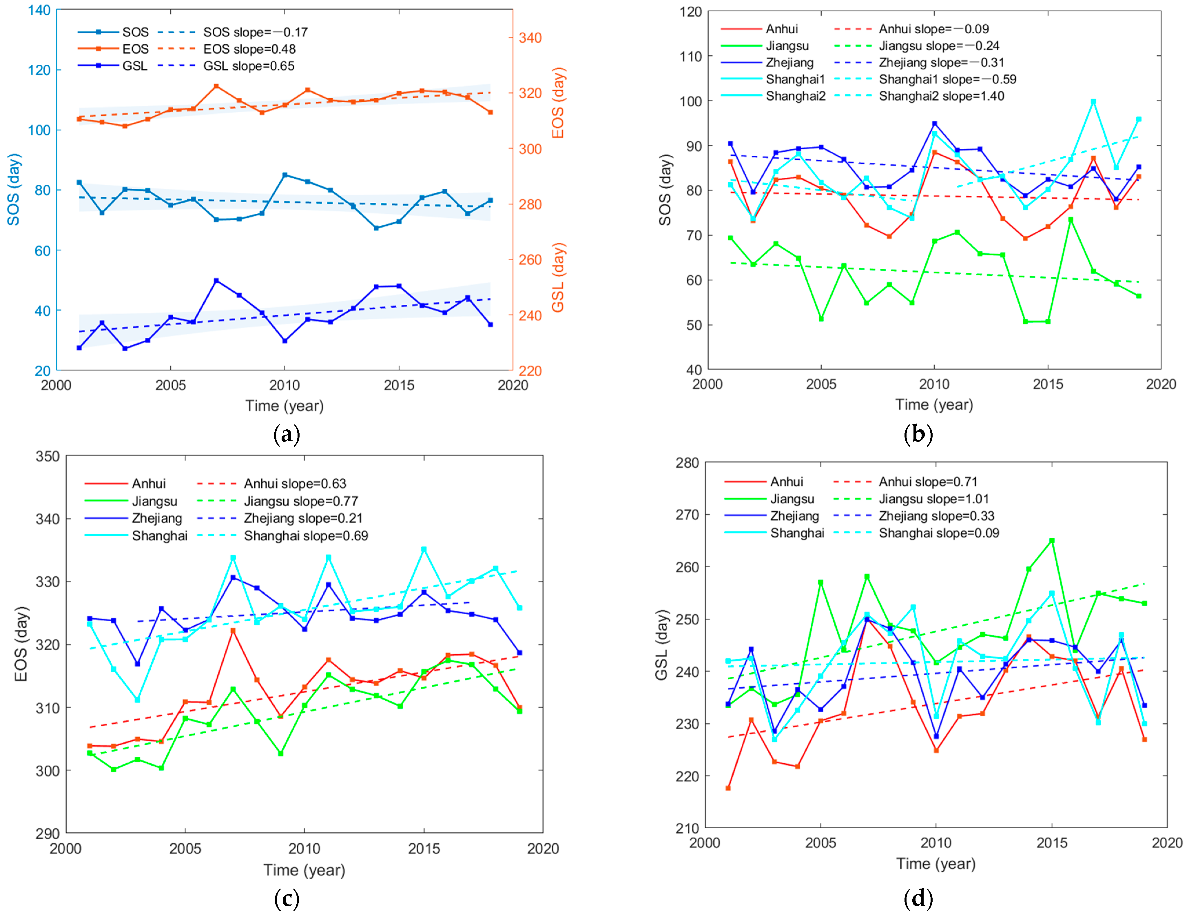
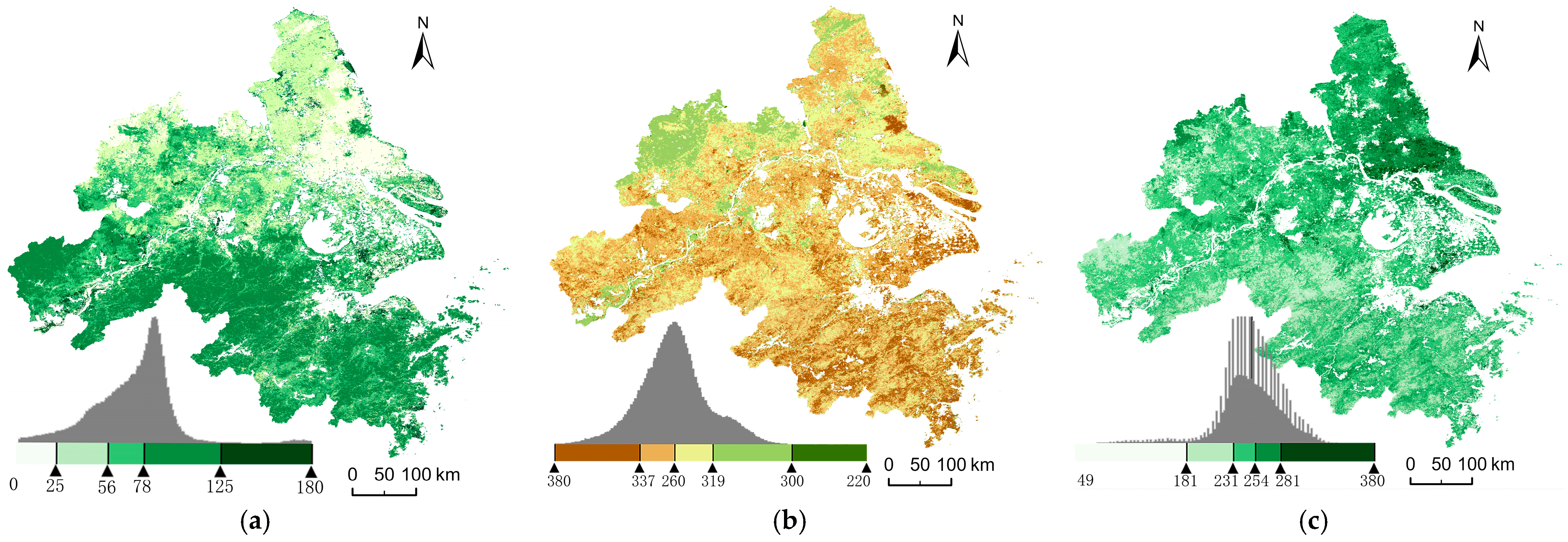
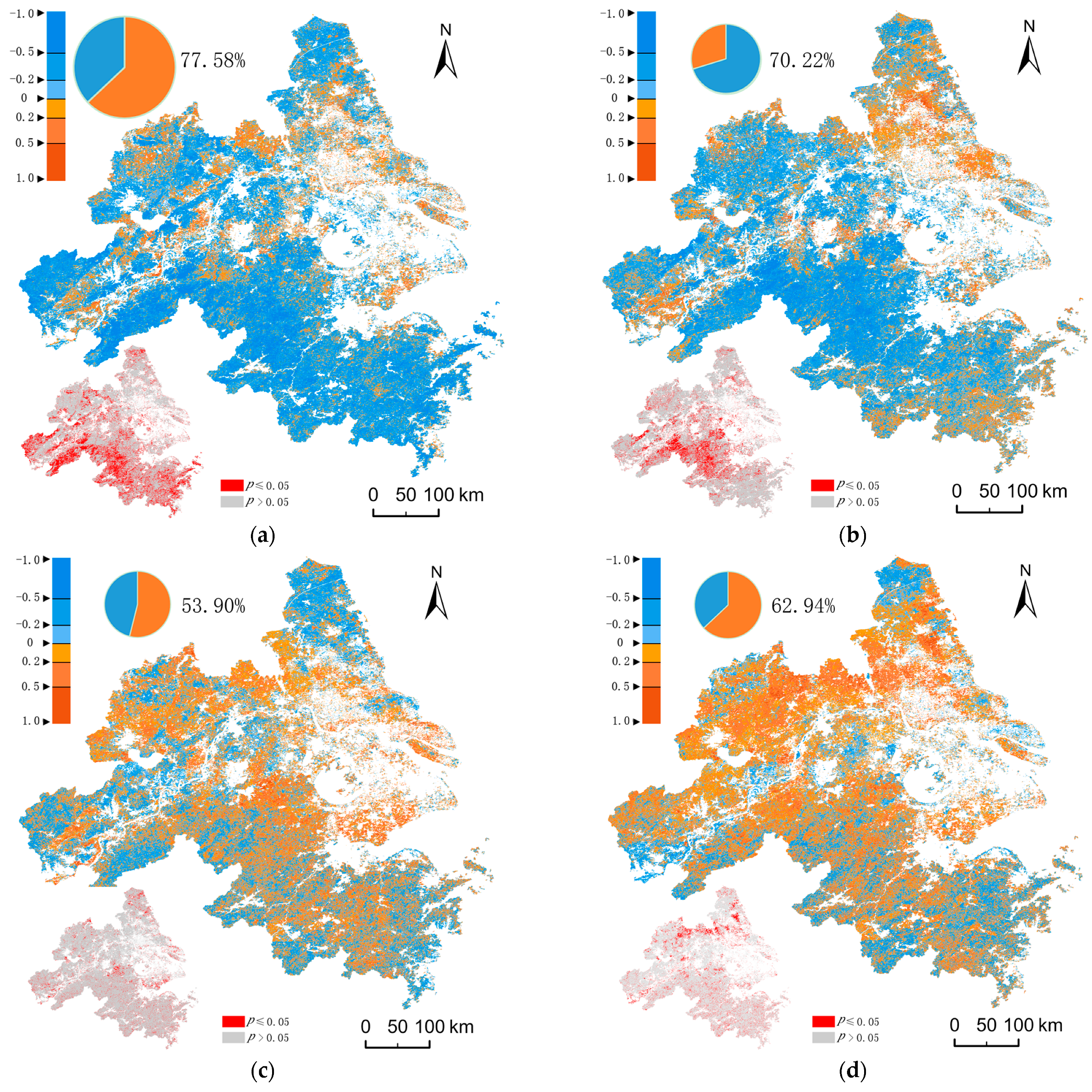
3.1. Spatiotemporal Variation Characteristics of Phenology

This paper discusses the temporal and spatial variation characteristics of phenology from three dimensions, namely time, plane and elevation. From the perspective of time (Figure 2a), it can be seen that the phenological index of the Yangtze River Delta fluctuates from 2001 to 2019, the advance of SOS is insignificant (p > 0.05) at 0.17 days per year and the EOS shows a significant delay (p < 0.01) of 0.48 days per year, and GSL is prolonged by 0.65 days per year (p < 0.05). In the past 19 years, the maximum difference between SOS is about 17.68 days, the maximum difference between EOS is 14.43 days and the maximum difference between GSL is about 24.49 days. The latest SOS and shortest GSL occurred in 2010, and relatively longer GSL occurred in 2007 and 2014.
The paper analyzed the characteristics of phenological change at provincial scale (Figure 2b–d) and found that the SOS in Anhui, Jiangsu and Zhejiang has an insignificant advance (p > 0.05) among which Anhui is the weakest with an average slope of 0.09 days per year. Jiangsu advances 0.24 days per year, while Zhejiang is relatively higher with 0.31 days per year. The minimum annual average difference (16.8 days) of SOS over the past 19 years was found in Zhejiang. The SOS in Shanghai, on the other hand, experienced a sudden change from 2009 to 2011, with an insignificant downward trend before 2009 (slope = −0.59, p > 0.05) and an upward trend after 2011 (slope = 1.40, p > 0.05). On the whole, SOS in Shanghai lagged by 0.59 days per year in the past 19 years (p > 0.05), and the average difference between the lowest and highest value is about 26 days. According to the annual average of SOS, Jiangsu has the earliest starting point of plant growth, followed by Anhui, Shanghai and Zhejiang. The average annual SOS difference among provinces ranged from 1.36 to 23.38 days. EOS in all provinces showed a delayed change trend. The delays in Anhui, Jiangsu and Shanghai are similar and significant (p < 0.01), about 0.63–0.77 days per year, but the changes in Zhejiang are relatively stable and insignificant (slope = 0.02, p > 0.05) with a maximum annual difference of 13.71 days. If the mutation time before 2003 and after 17 years is removed, the slope of the trend line is 0.21 days per year (p > 0.05). The EOSs in Zhejiang and Shanghai have fluctuated in recent 19 years; the intersection point appeared in 2009. In addition, EOS presents a clustering phenomenon, which is represented by Zhejiang and Shanghai and Jiangsu and Anhui. GSLs at provincial scales have insignificant delay trends (p > 0.05), except for Jiangsu. The slope value of Shanghai is the smallest (slope = 0.09), and Jiangsu has the strongest and significant change rate (slope = 1.01, p < 0.05). In terms of average GSL, Jiangsu has the longest growing season, while Anhui has the shortest growing season.
From the perspective of two-dimensional plane space (Figure 3), the spring phenology starts earlier in the northern part of the Yangtze River Delta than in the southern part. Similarly, the EOS of vegetation concentrated in the southern part is later than that in the northern part and is especially later than that in the northwest region. The Yangtze River becomes the dividing line regarding the north–south difference of SOS or EOS in the study area. The GSL value is mainly concentrated between 200 and 300, and the growing season in northern Jiangsu is obviously longer than that in the southern part of the Yangtze River Delta, especially the southwestern part.
The Yangtze River Delta is dominated by plains and hills, but there are mountains in western and southern Anhui and southwestern Zhejiang. From the perspective of elevation, with an increase in altitude, SOS is delayed, EOS advances and GSL is shortened (p < 0.01). For every 100 m increase, SOS is delayed by 1.44 days, EOS advances by 2.48 days and GSL is shortened by 1.05 days (Figure 4a).
According to the six grades classified in this paper (Figure 4b–d), SOS strictly adheres to the characteristic of increasing SOS value (delayed SOS) with increasing altitude. Except for the area below 100 m (no mutation), the mutation points of SOS with other altitude grades occurred at the beginning and end of time series; the EOS and GSL of individual altitude grades have mutation, but the trend is not significant (p > 0.05). Therefore, this paper only analyzes the overall trend of each elevation level. From 2001 to 2019, SOS shows an insignificant advance in all grades (p > 0.05), EOS shows an advancing trend between 200–1000 m and the other three stages are delayed. That is, in the altitude area less than 200 m and greater than 1000 m, delayed EOS appeared. The EOS of the regions with elevation below 100 m has a very significant trend of delay (p < 0.01). Moreover, EOS values above 200 m follow the trend of decreasing as the elevation increases, while the EOS values below 200 m have the opposite characteristics; that is, EOS values below 100 m are earlier than those between 100 and 200 m, and EOS values below 200 m are earlier than those between 200 and 1000 m. Except for 200–500 m, the other grades of GSL show an insignificant extension trend, and the prolongation is very significant below 100 m (p < 0.01). In conclusion, the changes in phenology, especially in EOS and GSL, are more obvious in areas where human activities are concentrated.

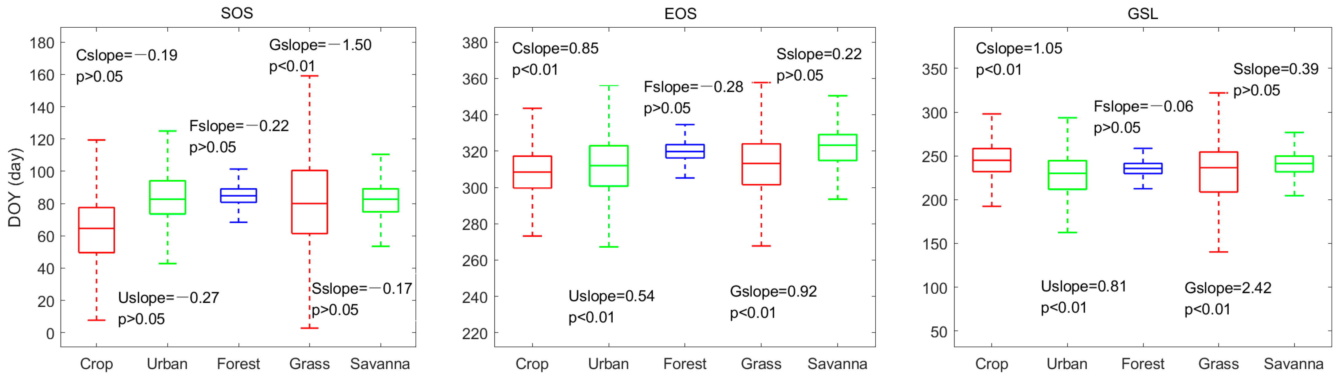
3.2. Phenological Characteristics of Different Land Cover Types

From Figure 5, we can see that the vegetation SOSs of five LC types and times are negatively correlated in the past 19 years and are advanced in all of those types. SOS of grassland significantly advanced 1.50 days per year (p < 0.01), followed by build-up areas (urban) and forests (p > 0.05). Except for the insignificant advance and shortening of forests (p > 0.05), the EOS and GSL of all other LC types are delayed. Grassland was delayed the most with a 0.92 average slope of EOS and a GSL slope of 2.42, followed by cropland (EOS slope = 0.85 p < 0.01; GSL slope = 1.05, p < 0.05) and build-up areas (EOS slope = 0.54 and GSL slope = 0.81). EOS and GSL of savannas were insignificantly delayed and prolonged (p > 0.05).
The phenology of cropland started earliest, followed by build-up areas and savannas. The SOS and EOS of forests are both later, but the value is the most concentrated in the study area, while grassland has the widest range of SOS and EOS. The vegetation GSL in build-up areas (mean) is shorter than that of forests and savannas. The GSL of grassland has great difference, but its mean value is smaller than that of cropland. Overall, the growing season of cropland is longer.

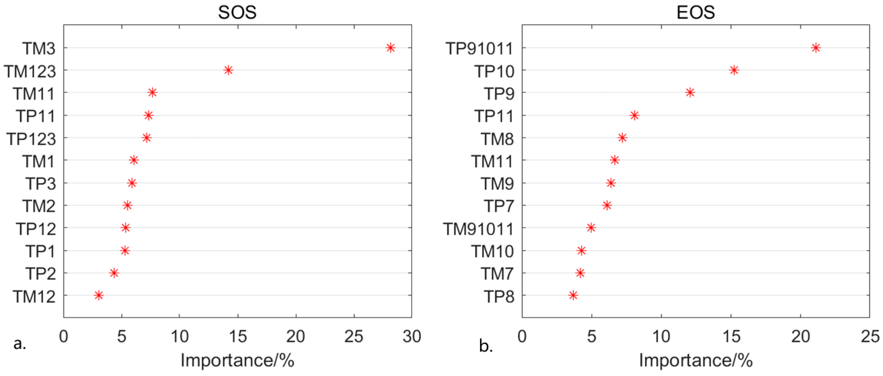
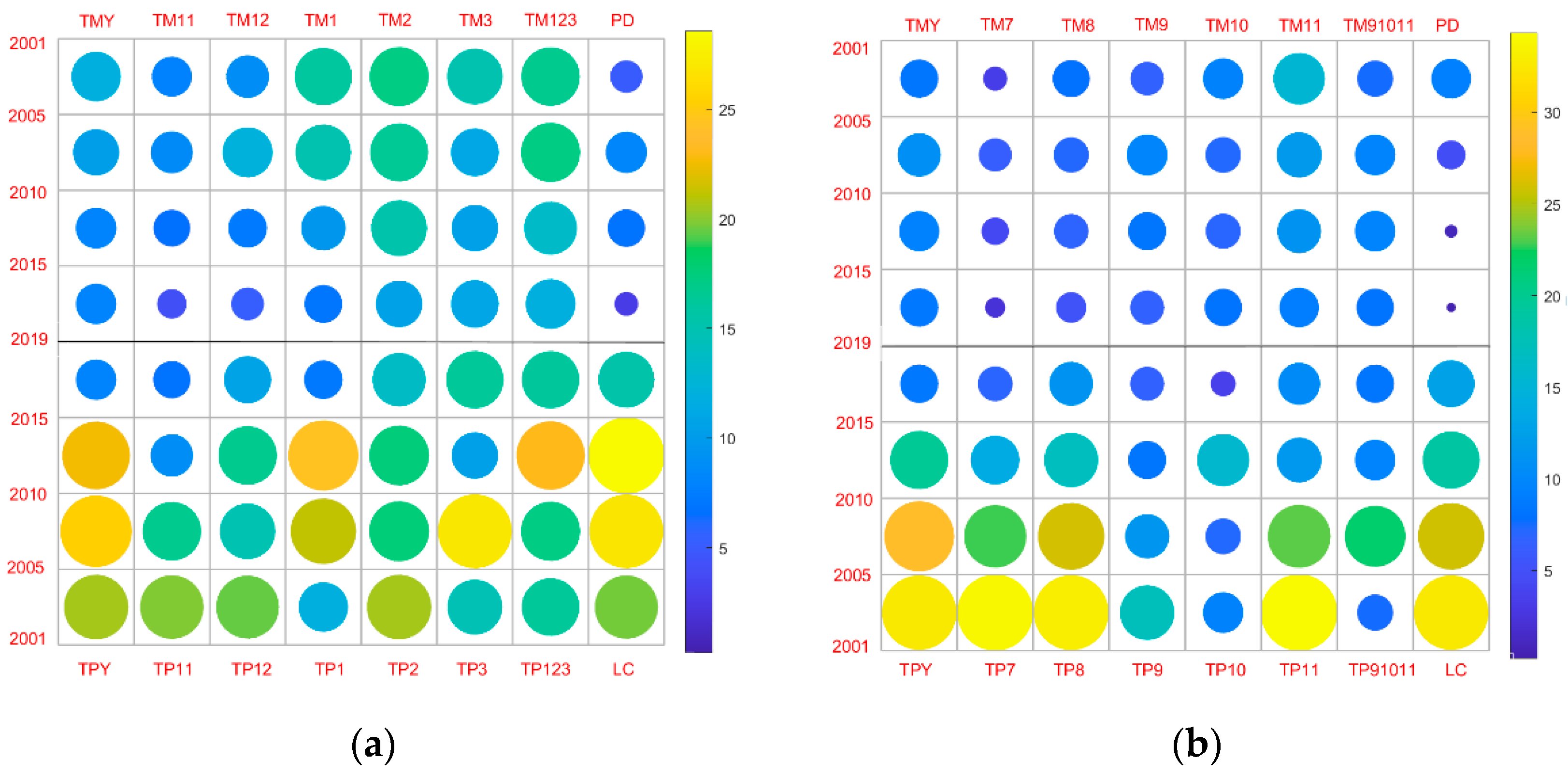
3.3. Relationship between Phenology and Climate

Numerous studies have shown that temperature and precipitation are the main controlling factors affecting the interannual variation of phenology. First, the paper analyzed the relationship between phenology and annual average precipitation and temperature (Figure 6). GSL is calculated from EOS and SOS, so this paper only explains the climate-driven relationship between EOS and SOS. The results show that SOS has an obvious negative correlation with temperature (Figure 6a) and precipitation (Figure 6b). The proportion of pixels with negative correlation to pixels in the whole experimental area is 77.58% (Figure 6a) and 70.22% (Figure 6b). The negative correlation is stronger in the southwest of experimental area, but relatively weak in the northwest and south of Jiangsu province. However, in the eastern and northeastern parts, positive correlations prevail. EOS is mainly positively correlated with annual average precipitation and temperature, with the highest correlations being 0.86 and 0.89, respectively. The positive correlation areas are mainly concentrated in the northern mountain areas of Anhui and southwestern Zhejiang, but the proportion of significant areas is not high. In general, the correlation between SOS and annual average temperature is greater than that of precipitation, while the correlation between EOS and annual average precipitation is stronger than that of temperature, and the correlation between EOS and climate factors (annual average temperature and precipitation) is weaker than that of SOS.
The response of preseason temperature and precipitation to phenology are analyzed using the random forest method. It can be seen from Figure 7 that SOS is mainly affected by temperature (importance = 65.09%). In particular, the temperature in March is the most important (importance = 27.8%) and has a significant negative correlation with SOS (Pearson = 0.681, p < 0.01). The average temperature from January to March is the second-most important factor for SOS. SOS in January, February and March is mainly affected by temperature. In November and December, there is not much difference between the contribution of temperature and precipitation to phenology, meaning SOS in November and December is influenced by both temperature and precipitation, but none of them pass the significance test (p > 0.05). EOS is mainly driven by precipitation (importance = 62.61%), especially the average precipitation from September to November (Pearson = 0.684, p < 0.01). During these three months, the most important factor is precipitation in October, followed by September. In July, September, October and November, precipitation is more important than temperature, while in August, temperature is more important but not significant (p > 0.05).

3.4. Spatial Heterogeneity and Its Driving Factors

The contribution of the temperature from November to February (TM11–TM2) to SOS gradually increased, and the highest contribution value is concentrated in February (Figure 8a). Meanwhile the contribution of the temperature from July to November (TM7–TM11) to EOS also shows a gradually increasing trend, and the month with highest contribution value is November (Figure 8b). This indicates that in the first month of the season, temperature contributed the most to SOS, and the highest-contributing month to EOS is the last month of the season. However, the relationship between preseason precipitation (TP11–TP2 and TP7–TP11) and heterogeneity of phenology is more complicated. The highest contribution to SOS of the four periods falls in February, March, January and March, respectively, while the highest contribution to EOS mainly falls in November and August. In particular, EOS is not only affected by midseason precipitation but also by preseason precipitation.
In addition, PD has a small impact on heterogeneity of phenology in the four time periods, the highest is 9.15% in 2001–2005, but the contribution of LC is as high as 34.06%. Overall, the effect of precipitation on heterogeneity of phenology is greater than that of temperature. For SOS, the contribution of LC is higher than that of temperature and slightly lower than that of precipitation. For EOS, the contribution of LC is higher, and the influence of the yearly average precipitation on the spatial heterogeneity of phenology is also high. Moreover, the combined effect of factors is much larger than the independent effect of each, indicating that the spatial heterogeneity of phenology is not caused by a single factor.

4. Discussion

4.1. Phenological Change Characteristics

In the terms of temporal variation characteristics, the trend of vegetation phenology in the Yangtze River Delta is consistent with previous research [16,47]; that is, SOS has an advancing trend from 2001 to 2019, while EOS is delayed and GSL is prolonged. Due to different data sources, periods and different research objects, the ranges of SOS and EOS value deviate slightly from the conclusions of Ding [16] and Han [48]. The SOS has been delayed since 2008 and peaked in 2010, resulting in the shortest GSL in 2010. A possible reason is that the temperature dropped sharply in 2008 compared with 2007, and this drop continued until 2011. At the same time, the precipitation increased from 2008 to 2010, but in 2011, it started to decrease. In addition, spring phenology has a significant correlation with the average temperature in January to March, and the correlation is also significant between spring phenology and average temperature in March, which are basically consistent with the conclusion of Zheng et al. [47].
The inconsistency of land cover types in various provinces has become one of the main reasons for the spatial heterogeneity of phenology, and the distribution of climate and land cover types comprehensively determines the differences in phenology. In Anhui and Jiangsu Provinces, the characteristics of cropland phenology play a major role in the conclusion that “SOS of Anhui and Jiangsu is earlier than that of Zhejiang and Shanghai”. Especially in the northern part of Jiangsu, the proportion of cropland is relatively larger and the SOS of cropland is the earliest, which led to the earlier SOS in Jiangsu than in other provinces. At the same time, cropland is also the main reason why the GSL of Jiangsu is longer than that of Zhejiang. The three provinces and Shanghai show the characteristics of double-clustering on EOS, which follows the principle of geographical similarity. In terms of latitude, although EOS advances with the increase in latitude at the provincial scale, SOS does not follow this rule. This is probably because the latitude and longitude spans of the study area are not large and their influence on phenology is less than that of land cover type, so their influence is not obvious.
As one of the highly developed cities, SOS value in Shanghai was less than 90 in all years except 2017 and 2019, which is consistent with previous research [16,48]. However, the possible reason for the interannual delay trend of SOS is that Shanghai is a coastal city which is located in the Yangtze River estuary. Firstly, the differences of land use and microclimate will be influenced by artificial and sea environment, and studies [21,46] believe that the microclimate can change phenological characteristics. Secondly, other studies pointed out that salting inhibited germination and leaf spreading [61,62] and caused increased asynchrony between individual pieces of vegetation [63]. The degree of saltiness in soil varies from year to year, and there is a possibility of residual accumulation of saltiness, which results in the delayed SOS of regional vegetation. Thirdly, individual differences among different species, extreme weather, human activities or environmental pollution may affect urban vegetation phenology [9,64,65]. Artificial vegetation is the main vegetation in Shanghai, and the degree of artificial management and protection are also factors affecting phenology. In addition, Li [4] and Wang [13] also pointed out that due to the complexity of phenology, the phenology of some cities would show opposite phenomena.
The results of phenology in the altitude dimension are that SOS is delayed, EOS is advanced and GSL is shortened with the increase in altitude, which is similar to the conclusions of Liu et al. [11] and Jeffery et al. [43]. However, due to the difference in research area, geographical environment and altitude, there are still differences in the value of the amplitude and trend of change. The conclusion of advanced SOS at different altitude grades is consistent with previous studies [17,20,43,66]. A phenology study of the European Alps showed that although EOS was advanced by 0.69 days per year on average [66], the results of EOS were different at different altitudes, and EOS was delayed between 1400 m and 1800 m. However, above 2000 m, EOS was advanced [43]. This is similar to the conclusion in this paper that the postponement trend is found above 1000 m. Insignificant fluctuation is likely to be caused by the insignificant climate change in recent years in experimental area and the stronger adaptation and regulation effect of forests on climate. EOS change below 100 m is significant; the main reason is the joint effect of climate and human activities because the region below 100 m is the area with intense human activities. Advanced EOS between 200 m and 1000 m may be caused by comprehensive factors such as local climate, environment, human activity and forest species types, such as terraced fields and economic forests.

4.2. Impacts of Land Cover Type on Phenology

The SOS and EOS values at different times are dependent on the type of land cover. In the past 19 years, the SOS of vegetation of the five land cover types in this paper all showed an earlier trend, but the amplitudes were different. Among them, the start time of phenology in build-up areas advanced by 0.27 days per year. A possible reason for this is that the vegetation in build-up areas is more severely affected by human activities and climate, such as artificial cultivation. This result is lower than the result of SOS trend in suburbs, while the slope of EOS in build-up area is 0.54 days per year, which is similar to the result (0.56 days per year) in suburban areas found by Ding [16]. Possible reasons are that different resolutions and data sources, mixed pixels and extraction methods may lead to different results. Additionally, different regional definitions are the key reasons for different results. In this study, vegetation in build-up areas does not have the longest growing season. This conclusion is different from the conclusion of Zhang [15] that urban growth season length is second only to cropland, which is mainly due to the different geographical environment and regional definition. Firstly, this paper does not include the urban core because of the coarse resolution of LC and phenology data. Secondly, the study area is dominated by subtropical monsoon climate, including some temperate and subtropical transitional regions, which is different from other research areas.
The conclusion that the SOS and EOS of grassland are earlier than that of forest is similar to that of Wang [49]. Meanwhile, the reason why grassland has a longer SOS range in this study area is that there are fewer natural grasslands in this experimental area, and artificial grassland is greatly affected by grassland type and artificial conservation. The cropland has the earliest phenology and the longest growing season, which is related to the fact that cropland has multiple crop rotation. In Anhui and northern Jiangsu, it is dominated by two rounds of crops. The conclusion that cropland has the longest growing season is consistent with other research [2,4,15,16]. It is interesting that the EOS of forests shows an overall advancing trend over time which is delayed first and then advances. A possible reason is that the forests in this experimental area are located in the mid-altitude mountainous areas of southwest Anhui and Southwest Zhejiang. EOS between 200–1000 m shows an advance trend, and this area occupies a large proportion of the forest area. In addition, there are plantation forests and economic forests, such as oil palm and bamboo, in the mountainous areas of western and southern Anhui, as well as in the mountainous areas of southwest Zhejiang. In addition, there are terraces under human activities in this area.
The relationship between land cover type and phenology was studied by Qiu [21], and it was concluded that different land cover has different phenological characteristics, which is consistent with the research in this paper. Land cover types have a great impact on the spatial heterogeneity of phenology due to their different phenological characteristics and may also have an impact on the temporal change of phenology. It is found by the random forest method that the importance of land cover on phenology is much larger than that of climate in this region spatiotemporal detection. According to the statistical data of land cover types, they changed from 2001 to 2019. Overall, the area of forest, grassland and build-up area show an increasing trend, and the largest increase in proportion of build-up area is about 58.3%. The rapid expansion of urban land is consistent with the research of [67]. The area of shrubland is the least, and the savanna increased and then decreased from 2001 to 2010, with the change being within 5%. Cropland area decreased gradually before 2015 and increased slightly from 2015 to 2019, which may be related to China’s policy of returning housing to farmland. The transfer of land cover types from 2001 to 2019 is shown in Figure 9. On the whole, the area of each land use type fluctuates, which indirectly leads to the interannual fluctuation of phenology. However, since the area of land use itself is larger than the changing area, its phenological characteristics still maintain and control the phenological change characteristics of the study area. The build-up area with the largest increase also presents the characteristics of SOS advance and EOS delay. It is worth noting that land use or land cover types include not only the five types mentioned in the paper, but also water bodies, etc. Since the study in this paper mainly focuses on the phenology of vegetation, other types are not objects of concern in this paper. Meanwhile, it can be seen from Figure 9 that shrubland area is very small, and the phenology of shrubland is not studied in detail in this paper. In addition, due to the impact of resolution, there are likely uncertainties in the amount of land transfer, but the change trend is worthy of reference.

4.3. Effects of Population Density and Land Surface Temperature on Phenology

In view of the fact that population density [48,68] and surface temperature [4] have been closely related to urban phenology in previous studies, supplementary analyses was made in this paper. From the perspective of interannual variation trend (Figure 10a), GSL in build-up areas (non-core urban) showed a significant positive correlation with daytime surface land temperature (DLST) (R2 = 0.30 p < 0.05), but there was insignificant positive correlation between GSL and nighttime surface land temperature (NLST) (R2 = 0.09, p > 0.05). The result is consistent with previous research. That is, the farther away from the city, the weaker the relationship between LST and phenology. When the distance from the city was greater than 6 km [48], or even more than 15 km [68], the relationship between LST and phenology was not obvious. In addition, from the perspective of p value, NLST is not the main factor of phenological fluctuation in build-up areas. PD showed an increasing trend, and there is an insignificant negative correlation with SOS (R2 = 0.13, p > 0.05) and significant positive correlation with EOS (R2 = 0.48, p < 0.01) and GSL (R2 = 0.52, p < 0.01). This is consistent with the conclusion that population density is related to urban phenology [48,68]. Due to the data’s resolution and the characteristics of phenological data sources, the central area of the city is not included in the build-up areas in this paper, which is also a possible reason why the correlation between the phenology of urban area and PD and LST is lower than in previous studies.
The results (Figure 10b) show that the contribution of temperature (TM) and precipitation (TP) to heterogeneity of phenology in build-up areas is higher than that of PD; the contribution of NLST is greater than that of DLST. The contribution of NLST to SOS heterogeneity is the highest, while the contribution of TM to EOS is the highest, but the overall contributions are both less than 14%. NLST is one of factors influencing the non-core urban phenology of spatial heterogeneity, but the PD is not a key element. The reason why PD has little influence on spatial heterogeneity may be that the PD of non-core urban areas itself has little heterogeneity. This also indirectly proves that urban areas, based on classification, are less sensitive to phenology [69].

5. Conclusions

The paper analyzed the phenological change in the Yangtze River Delta from the three dimensions of time, plane space and elevation by using MODIS phenology, meteorological data, land surface temperature, land use and population density data. On this basis, the main driving factors of interannual variation and spatial heterogeneity of phenology and their response mechanisms were analyzed using the random forest and geographic detector methods. Furthermore, the relationship between phenology and PD and LST are studied in non-core urban areas. The conclusions are as follows:
(1)
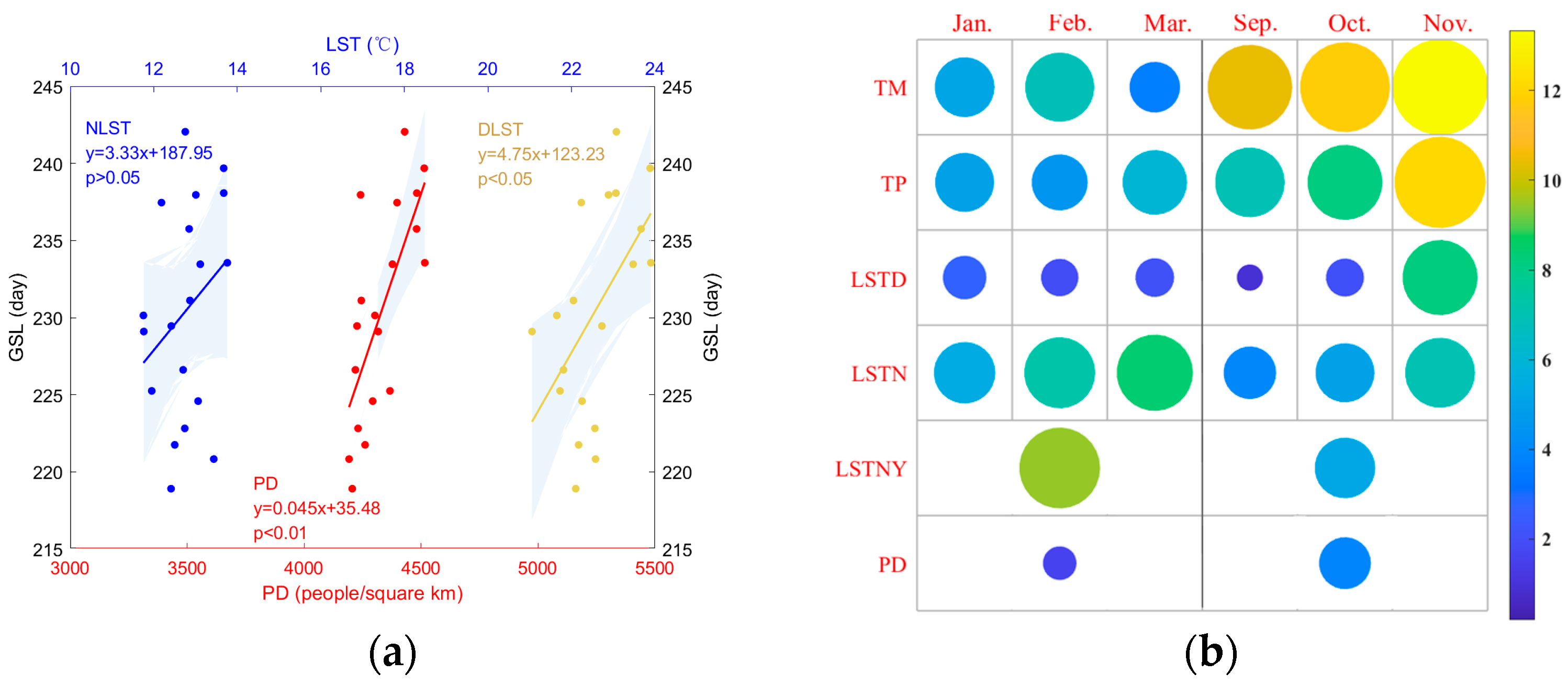
SOS in the Yangtze River Delta shows an insignificant advance (p > 0.05) of 0.17 days per year, EOS is significantly delayed (p < 0.01) by 0.48 days per year and GSL is prolonged by 0.65 days per year (p < 0.05). SOS has an obvious negative correlation with temperature and precipitation, and EOS has a positive correlation with them. Preseason temperature has a greater contribution to SOS, while preseason precipitation is a major factor of EOS. Two months before the growing season, it is jointly affected by temperature and precipitation.
(2)
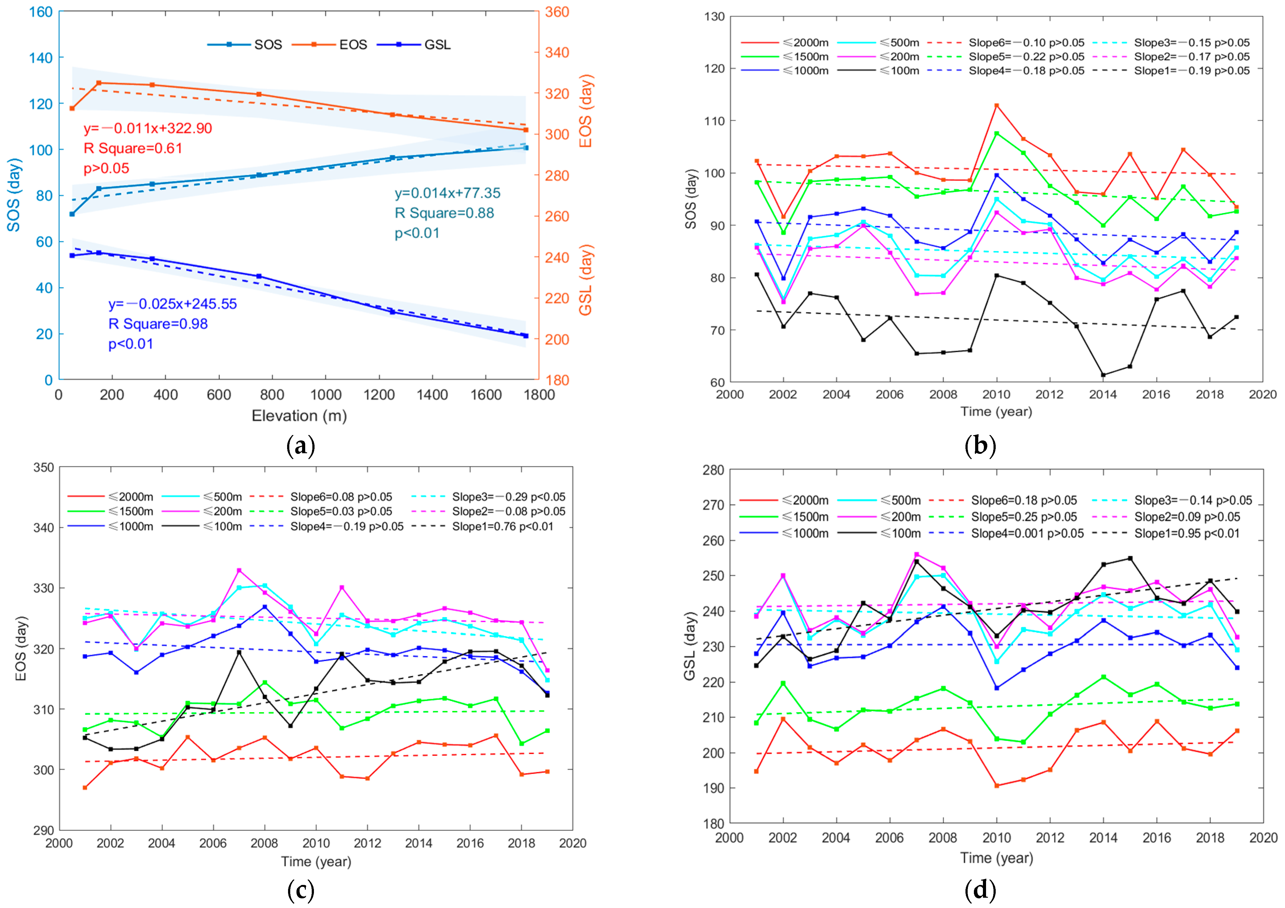
Large divergent responses of vegetation phenology to spatial distribution and elevation grades are found. The variation characteristics of SOS and GSL in the Yangtze River Delta and its provinces do not obey the rules of latitude variation. EOS values above 200 m follow the trend of decreasing as elevation increases, while the EOS values below 200 m have the opposite characteristic. In addition, the changes in phenological indexes of vegetation below 100 m are the most obvious.
(3)
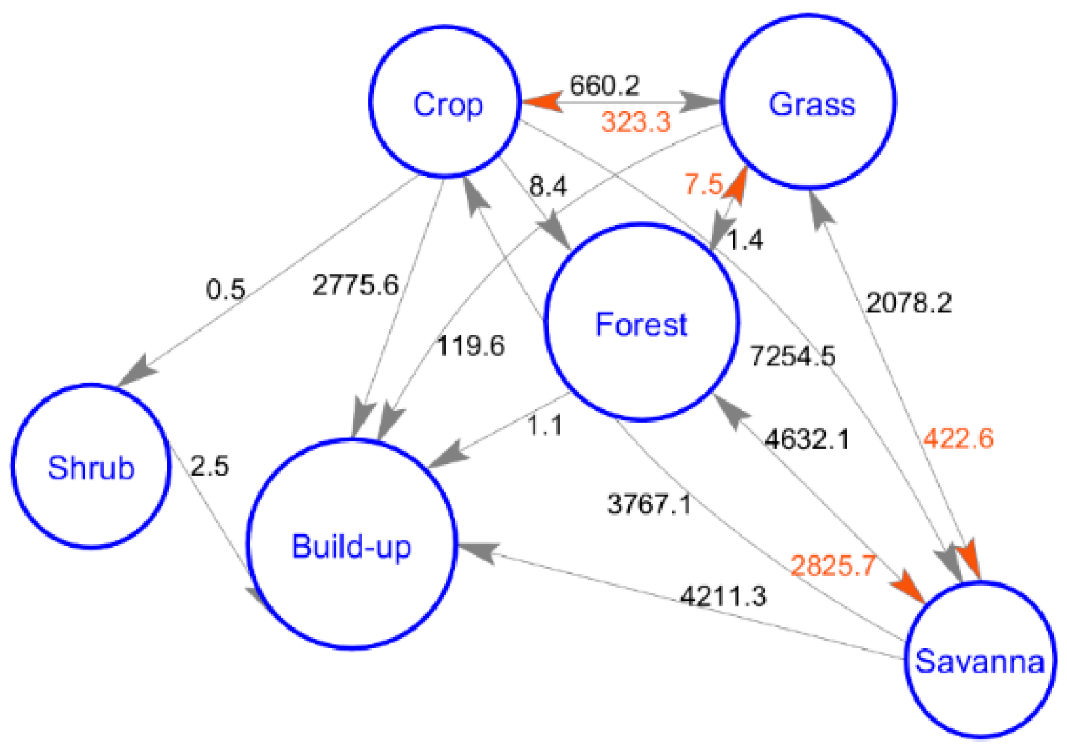
The phenology of vegetation is different in the five LC types. In addition, the contribution of LC types to the spatial change of phenology is greater than that of temperature and precipitation, and the transfer of LC may also be one factor driving the interannual change in phenology.
(4)
In non-core urban areas, NLST has a relatively large contribution to the spatial heterogeneity of phenology. Although PD has a strong correlation with GSL, it contributes little to spatial heterogeneity.
It is worth noting that due to the limitations of data sources, the loss of urban center areas in this study will have a certain impact on the research results, especially the statistics of vegetation phenology in build-up areas. As the next step, high-resolution images will be introduced for research and supplement. The interannual change of the LC area of each type is less than the area of LC itself, and the interannual change of PD in non-urban areas is small, so the drive of LC and PD on phenology is not quantified when analyzing change drivers of temporal heterogeneity. The follow-up must take urban area as the main research object to study the two factors and their response relationship. Finally, the driving forces of each LC type are temporarily not within the scope of this paper, and other influencing factors (accumulated temperature, photoperiod, carbon dioxide concentration, etc.) are not taken into account. This approach will be further refined in the follow-up research.

Author Contributions

Conceptualization, C.Y. and M.Z.; formal analysis and data curation, C.Y.; methodology and supervision, D.P.; writing—original draft, C.Y. and K.D.; visualization and investigation, K.D.; writing—reviewing and editing, D.P., L.J., J.L., X.Q. and M.Z. All authors have read and agreed to the published version of the manuscript.

Funding

This research was supported by the Key Project of Natural Science Research of the Anhui Provincial Department of Education (Grant No. KJ2020A0721, Grant No. KJ2020A0722); Anhui Province Universities Outstanding Talented Person Support Project (Grant No. gxyq2019093); Chuzhou Science and Technology Bureau guiding project (Grant No. 2021ZD008); Key Project of Research and Development in Chuzhou Science and Technology Program (No. 2020ZG016); and Innovation program for Returned Overseas Chinese Scholars of Anhui Province (No. 2021LCX014).

Data Availability Statement

Not applicable.

Acknowledgments

We are thankful for all of the helpful comments provided by the reviewers and editors.

Conflicts of Interest

The authors declare no conflict of interest.

References

  1. White, M.A.; Nemani, R.R.; Thornton, P.E.; Running, S.W. Satellite evidence of phenological differences between urbanized and rural areas of the Eastern United States deciduous broadleaf forest. Ecosystems 2002, 5, 260–273. [Google Scholar] [CrossRef]
  2. White, M.A.; Beurs, K.M.D.; Didan, K.; Inouye, D.W.; Richardson, A.D.; Jensen, O.P.; O’keefe, J.; Zhang, G.; Nemani, R.R.; van Leeuwen, W.J.D.; et al. Intercomparison, interpretation, and assessment of spring phenology in North America estimated from remote sensing for 1982–2006. Glob. Change Biol. 2009, 15, 2335–2359. [Google Scholar] [CrossRef]
  3. Richardson, A.D.; Keenan, T.F.; Migliavacca, M.; Ryu, Y.; Sonnentag, O.; Toomey, M. Climate change, phenology, and phenological control of vegetation feedbacks to the climate system. Agric. For. Meteorol. 2013, 169, 156–173. [Google Scholar] [CrossRef]
  4. Li, X.; Zhou, Y.; Asrar, G.R.; Mao, J.; Li, X.; Li, W. Response of vegetation phenology to urbanization in the conterminous United States. Glob. Change Biol. 2017, 23, 2818–2830. [Google Scholar] [CrossRef]
  5. Wang, Y.; Xu, W.; Yuan, W.; Chen, X.; Zhang, B.; Fan, L.; He, B.; Hu, Z.; Liu, S.; Liu, W. Higher plant photosynthetic capability in autumn responding to low atmospheric vapor pressure deficit. Innovation 2021, 2, 100163. [Google Scholar] [CrossRef]
  6. Chang, Q.; Xiao, X.; Jiao, W.; Ling, D.; Zeng, Z.; Qin, Y. Assessing consistency of spring phenology of snow-covered forests as estimated by vegetation indices, gross primary production, and solar induced chlorophyll fluorescence. Agric. For. Meteorol. 2019, 275, 305–316. [Google Scholar] [CrossRef]
  7. Qiu, T.; Song, C.; Li, J. Deriving annual double-season cropland phenology using Landsat imagery. Remote Sens. 2020, 12, 3275. [Google Scholar] [CrossRef]
  8. Cui, L.; Shi, J.; Du, H. Advances in remote sensing extraction of vegetation phenology and its driving factors. Adv. Earth Sci. 2021, 36, 9–16. [Google Scholar] [CrossRef]
  9. Piao, S.; Fang, J.; Zhou, L.; Ciais, P.; Zhu, B. Variations in satellite-derived phenology in China’s temperate vegetation. Glob. Change Biol. 2006, 12, 672–685. [Google Scholar] [CrossRef]
  10. Ge, Q.; Wang, H.; Rutishauser, T.; Dai, J. Phenological response to climate change in China: A meta-analysis. Glob. Change Biol. 2015, 21, 265–274. [Google Scholar] [CrossRef] [PubMed]
  11. Liu, X.; Chen, Y.; Li, Z.; Li, Y.; Zhang, Q.; Zan, M. Driving forces of the changes in vegetation phenology in the Qinghai-Tibet Plateau. Remote Sens. 2021, 13, 4952. [Google Scholar] [CrossRef]
  12. Jiao, F.; Liu, H.; Xu, X.; Gong, H.; Lin, Z. Trend evolution of vegetation phenology in china during the period of 1981–2016. Remote Sens. 2020, 12, 572. [Google Scholar] [CrossRef] [Green Version]
  13. Wang, X.; Du, P.; Chen, D.; Lin, C.; Zheng, H.; Guo, S. Characterizing urbanization induced land surface phenology change from time-series remotely sensed images at fine spatio-temporal scale: A case study in Nanjing, China (2001–2018). J. Clean. Prod. 2020, 274, 122487. [Google Scholar] [CrossRef]
  14. Shen, M.; Zhang, G.; Cong, N.; Wang, S.; Kong, W.; Piao, S. Increasing altitudinal gradient of spring vegetation phenology during the last decade on the Qinghai-Tibetan Plateau. Agric. For. Meteorol. 2014, 189, 71–80. [Google Scholar] [CrossRef]
  15. Zhang, Y.; Yin, P.; Li, X.; Niu, Q.; Wang, Y.; Cao, W.; Huang, J.; Chen, H.; Yao, X.; Yu, L.; et al. The divergent response of vegetation phenology to urbanization: A case study of Beijing city, China. Sci. Total Environ. 2022, 803, 150079. [Google Scholar] [CrossRef]
  16. Ding, H.; Xu, L.; Elmore, A.J.; Shi, Y. Vegetation Phenology Influenced by Rapid Urbanization of The Yangtze Delta Region. Remote Sens. 2020, 12, 1783. [Google Scholar] [CrossRef]
  17. Guo, J.; Liu, X.; Ge, W.; Ni, X.; Ma, W.; Lu, Q.; Xing, X. Specific Drivers and Responses to Land Surface Phenology of Different Vegetation Types in the Qinling Mountains, Central China. Remote Sens. 2021, 13, 4538. [Google Scholar] [CrossRef]
  18. Kelsey, K.C.; Pedersen, S.H.; Leffler, A.J.; Sexton, J.O.; Feng, M.; Welker, J.M. Winter snow and spring temperature have differential effects on vegetation phenology and productivity across plant communities. Glob. Change Biol. 2021, 27, 1572–1586. [Google Scholar] [CrossRef]
  19. Jia, W.; Zhao, S.; Zhang, X.; Liu, S.; Henebry, G.M.; Liu, L.L. Urbanization imprint on land surface phenology: The urban-rural gradient analysis for Chinese cities. Glob. Change Biol. 2021, 27, 2895–2904. [Google Scholar] [CrossRef]
  20. Tang, H.; Li, Z.; Zhu, Z.; Chen, B.; Zhang, B.; Xin, X. Variability and climate change trend in vegetation phenology of recent decades in the Greater Khingan Mountain area, Northeastern China. Remote Sens. 2015, 7, 11914–11932. [Google Scholar] [CrossRef] [Green Version]
  21. Qiu, T.; Song, C.; Li, J. Impacts of urbanization on vegetation phenology over the past three decades in Shanghai, China. Remote Sens. 2017, 9, 970. [Google Scholar] [CrossRef] [Green Version]
  22. Yang, K.; Sun, W.; Luo, Y.; Zhao, L. Impact of urban expansion on vegetation: The case of China (2000–2018). J. Environ. Manag. 2021, 291, 112598. [Google Scholar] [CrossRef] [PubMed]
  23. Ren, S.; Yi, S.; Peich, M.; Wang, X. Diverse Responses of Vegetation Phenology to Climate Change in Different Grasslands in Inner Mongolia during 2000–2016. Remote Sens. 2017, 10, 17. [Google Scholar] [CrossRef] [Green Version]
  24. Ren, S.; Qin, Q.; Ren, H.; Sui, J.; Zhang, Y. New model for simulating autumn phenology of herbaceous plants in the Inner Mongolian Grassland. Agric. For. Meteorol. 2019, 275, 136–145. [Google Scholar] [CrossRef]
  25. Cong, N.; Wang, T.; Nan, H.; Ma, Y.; Wang, X.; Myneni, R.B.; Piao, S. Changes in satellite-derived spring vegetation green-up date and its linkage to climate in China from 1982 to 2010: A multimethod analysis. Glob. Change Biol. 2013, 19, 881–891. [Google Scholar] [CrossRef]
  26. Li, P.; Zhu, Q.; Peng, C.; Zhang, J.; Wang, M.; Zhang, J.; Ding, J.; Zhou, X. Change in Autumn Vegetation Phenology and the Climate Controls From 1982 to 2012 on the Qinghai-Tibet Plateau. Front. Plant. Sci. 2020, 10, 1677. [Google Scholar] [CrossRef] [Green Version]
  27. Shen, M.; Piao, S.; Cong, N.; Zhang, G.; Jassens, I.A. Precipitation impacts on vegetation spring phenology on the Tibetan Plateau. Glob. Change Biol. 2015, 21, 3647–3656. [Google Scholar] [CrossRef] [PubMed] [Green Version]
  28. Tao, F.; Yokozawa, M.; Zhang, Z.; Hayashi, Y.; Ishigooka, Y. Land surface phenology dynamics and climate variations in the North East China Transect(NECT), 1982–2000. Int. J. Remote Sens. 2008, 29, 5461–5478. [Google Scholar] [CrossRef]
  29. Peng, S.; Piao, S.; Ciais, P.; Myneni, R.B.; Chen, A.; Chevallier, F.; Dolman, A.J.; Janssens, I.A.; Peñuelas, J.; Zhang, G.; et al. Asymmetric effects of daytime and night-time warming on Northern Hemisphere vegetation. Nature 2013, 501, 88–92. [Google Scholar] [CrossRef] [PubMed]
  30. Wan, S.; Xia, J.; Liu, W.; Niu, S. Photosynthetic overcompensation under nocturnal warming enhances grassland carbon sequestration. Ecology 2009, 90, 2700–2710. [Google Scholar] [CrossRef] [PubMed] [Green Version]
  31. Meng, F.; Zhang, L.; Zhang, Z.; Jiang, L.; Wang, Y.; Duan, J.; Wang, Q.; Li, B.; Liu, P.; Hong, H. Opposite effects of winter day and night temperature changes on early phenophases. Ecology 2019, 100, e02775. [Google Scholar] [CrossRef] [PubMed]
  32. Piao, S.; Tan, J.; Chen, A.; Fu, Y.; Ciais, P.; Qiang, L.; Janssens, I.A.; Vicca, S.; Zeng, Z.; Jeong, S.J. Leaf onset in the northern hemisphere triggered by daytime temperature. Nat. Commun. 2015, 6, 6911. [Google Scholar] [CrossRef] [PubMed] [Green Version]
  33. Fu, Y.H.; Piao, S.; Zhou, X.; Geng, X.; Hao, F.; Vitasse, Y.; Janssens, I.A. Short photoperiod reduces the temperature sensitivity of leaf-out in saplings of Fagus sylvatica but not in Horse chestnut. Glob. Change Biol. 2019, 25, 1696–1703. [Google Scholar] [CrossRef]
  34. Fu, Y.H.; Zhao, H.; Piao, S.; Peaucelle, M.; Peng, S.; Zhou, G.; Ciais, P.; Huang, M.; Menzel, A.; Peñuelas, J.; et al. Declining global warming effects on the phenology of spring leaf unfolding. Nature 2015, 526, 104–107. [Google Scholar] [CrossRef] [Green Version]
  35. Korner, C.; Basler, D. Phenology Under Global Warming. Science 2010, 327, 1461–1462. [Google Scholar] [CrossRef]
  36. David, B.; Christian, K. Photoperiod and temperature responses of bud swelling and bud burst in four temperate forest tree species. Tree Physiol. 2014, 34, 377–388. [Google Scholar] [CrossRef] [Green Version]
  37. Caffarra, A.; Donnelly, A.; Chuine, I. Modelling the timing of Betula pubescens budburst. II. Integrating complex effects of photoperiod into process-based models. Clim. Res. 2011, 46, 159–170. [Google Scholar] [CrossRef]
  38. Moon, M.; Richardson, A.D.; O’Keefe, J.; Friedl, M.A. Senescence in temperate broadleaf trees exhibits species-specific dependence on photoperiod versus thermal forcing. Agric. For. Meteorol. 2022, 322, 109026. [Google Scholar] [CrossRef]
  39. Meng, L.; Zhou, Y.; Gu, L.; Richardson, A.D.; Peñuelas, J.; Fu, Y.; Wang, Y.; Asrar, G.R.; de Boeck, H.J.; Mao, J.; et al. Photoperiod decelerates the advance of spring phenology of six deciduous tree species under climate warming. Glob. Change Biol. 2021, 27, 2914–2927. [Google Scholar] [CrossRef]
  40. Zohner, C.M.; Benito, B.M.; Svenning, J.C.; Renner, S.S. Day length unlikely to constrain climate-driven shifts in leaf-out times of northern woody plants. Nat. Clim. Change 2016, 6, 1120–1123. [Google Scholar] [CrossRef]
  41. Lv, A.L.; Huo, Z.G.; Yang, J.Y. Phenological Characteristics of Representative Woody Plants at Different Altitude Sites in Jinnan Region and Their Response to Climate Change. Chin. J. Agrometeorol. 2020, 41, 65–75. [Google Scholar] [CrossRef]
  42. Yuan, Q.L.; Yang, J. Phenological Changes of Grassland Vegetation and Its Response to Climate Change in Qinhai-Tibet Plateau. Chin. J. Grassl. 2021, 43, 32–43. [Google Scholar] [CrossRef]
  43. Thompson, J.A.; Paul, D.J. Assessing spatial and temporal patterns in land surface phenology for the Australian Alps (2000–2014). Remote Sens. Environ. 2017, 199, 1–13. [Google Scholar] [CrossRef]
  44. Jochner, S.; Menzel, A. Urban phenological studies- Past, present, future. Environ. Pollut. 2015, 203, 250–261. [Google Scholar] [CrossRef]
  45. Meng, L.; Mao, J.; Zhou, Y.; Richardson, A.D.; Jia, G. Urban warming advances spring phenology but reduces the response of phenology to temperature in the conterminous United States. Proc. Natl. Acad. Sci. USA 2020, 117, 201911117. [Google Scholar] [CrossRef]
  46. Zipper, S.C.; Schatz, J.; Singh, A.; Kucharik, C.J.; Townsend, P.A.; Loheide, S.P. Urban heat island impacts on plant phenology: Intra-urban variability and response to land cover. Environ. Res. Lett. 2016, 11, 054023. [Google Scholar] [CrossRef]
  47. Zheng, J.; Ge, Q.; Hao, Z.; Zhong, S.; Ma, X.; Zhang, X. Changes of spring phenodate in Yangtze River Delta region in the past 150 years. Acta Geogr. Sin. 2012, 67, 45–52. [Google Scholar] [CrossRef]
  48. Han, G.; Xu, J. Land Surface phenology and land surface temperature changes along an urban-rural gradient in Yangtze River Delta, China. Environ. Manag. 2013, 52, 234–249. [Google Scholar] [CrossRef]
  49. Wang, Y.; Xue, Z.; Chen, J.; Chen, G. Spatio-temporal analysis of phenology in Yangtze River Delta based on MODIS NDVI time series from 2001 to 2015. Front. Earth Sci. 2018, 13, 92–110. [Google Scholar] [CrossRef]
  50. Xiao, R.; Cao, W.; Liu, Y.; Lu, B. The impacts of landscape patterns spatio-temporal changes on land surface temperature from a multi-scale perspective: A case study of the Yangtze River Delta. Sci. Total Environ. 2022, 821, 153381. [Google Scholar] [CrossRef]
  51. Farr, T.G.; Rosen, P.A.; Caro, E.; Crippen, R.; Duren, R.; Hensley, S.; Kobrick, M.; Paller, M.; Rodriguez, E.; Roth, L.; et al. The shuttle radar topography mission. Rev. Geophys. 2007, 45, 361. [Google Scholar] [CrossRef] [Green Version]
  52. Sulla-Menashe, D.; Friedl, M.A. User Guide to Collection 6 MODIS Land Cover (MCD12Q1 and MCD12C1) Product; USGS: Reston, VA, USA, 2018; 18p. Available online: http://girps.net/wp-content/uploads/2019/03/MCD12_User_Guide_V6.pdf (accessed on 22 February 2022).
  53. Ji, Y.; Jin, J.; Zhan, W.; Guo, F.; Yan, T. Quantification of urban heat island-induced contribution to advance in spring phenology: A case study in Hangzhou, China. Remote Sens. 2021, 13, 3684. [Google Scholar] [CrossRef]
  54. Li, B.Y.; Pan, B.T.; Han, J.F. Basic terrestrial geomorphological types in China and their circum scriptions. Quat. Sci. 2008, 28, 535–543. [Google Scholar] [CrossRef]
  55. Liang, L.; Schwartz, M.D.; Fei, S. Validating satellite phenology through intensive ground observation and landscape scaling in a mixed seasonal forest. Remote Sens. Environ. 2011, 115, 143–157. [Google Scholar] [CrossRef]
  56. Zhang, X.; Friedl, M.A.; Schaaf, C.B. Global vegetation phenology from Moderate Resolution Imaging Spectroradiometer (MODIS): Evaluation of global patterns and comparison with in situ measurements. J. Geophys. Res. Biogeosci. 2015, 111, 367–375. [Google Scholar] [CrossRef]
  57. Wang, L.; De Boeck, H.J.; Chen, L.; Song, C.; Chen, Z.; McNulty, S.; Zhang, Z. Urban warming increases the temperature sensitivity of spring vegetation phenology at 292 cities across China. Sci. Total Environ. 2022, 834, 155154. [Google Scholar] [CrossRef]
  58. Mann, H.B. Nonparametric Tests Against Trend. Econometrica 1945, 13, 245–259. [Google Scholar] [CrossRef]
  59. Breiman, L. Random Forests. Mach. Learn. 2001, 45, 5–32. [Google Scholar] [CrossRef] [Green Version]
  60. Wang, J.; Xu, C. Geodetector: Principle and prospective. Acta Geogr. Sin. 2017, 72, 116–134. [Google Scholar] [CrossRef]
  61. He, B.; Cai, Y.; Ran, W.; Jiang, H. Spatial and seasonal variations of soil salinity following vegetation restoration in coastal saline land in eastern China. CATENA 2014, 118, 147–153. [Google Scholar] [CrossRef]
  62. Tian, J.; Cai, Y.; Zhao, X.; Xie, C. Phenological analysis and comparison of six greening trees between coastal island and inland, choosing Chongming island and Minghang area of Shanghai for an example. J. Shanghai Jiaotong Univ. 2015, 33, 71–79. [Google Scholar] [CrossRef]
  63. Zhao, X.; Shi, C.; He, B.; Ran, W.; Cai, Y. Spring phenological characteristics and phenophase classification of landscape greening tree species in Chongming Island of Shanghai. Chin. J. Ecol. 2013, 32, 2275–2280. [Google Scholar] [CrossRef]
  64. He, Z.; Du, J.; Chen, L.; Xi, Z.; Lin, P.; Zhao, M.; Fang, S. Impacts of recent climate extremes on spring phenology in arid-mountain ecosystems in China. Agric. For. Meteorol. 2018, 260–261, 31–40. [Google Scholar] [CrossRef]
  65. Yuan, M.; Zhao, L.; Lin, A.; Wang, L.; Li, Q.; She, D.; Qu, S. Impacts of preseason drought on vegetation spring phenology across the Northeast China Transect. Sci. Total Environ. 2020, 738, 140297. [Google Scholar] [CrossRef] [PubMed]
  66. Stöckli, R.; Vidale, P.L. European plant phenology and climate as seen in a 20-year AVHRR land-surface parameter dataset. Int. J. Remote Sens. 2004, 25, 3303–3330. [Google Scholar] [CrossRef]
  67. Yu, Z.; Chen, L.; Li, L.; Zhang, T.; Yuan, L.; Liu, R.; Wang, Z.; Zang, J.; Shi, S. Spatiotemporal Characterization of the Urban Expansion Patterns in the Yangtze River Delta Region. Remote Sens. 2021, 13, 4484. [Google Scholar] [CrossRef]
  68. Ding, H.; Bu, Y.; Xu, L. Spatial and temporal variation of the plant phenology and its response to the urbanization trend in the Yangtze River delta. J. Saf. Environ. 2021, 21, 1352–1360. [Google Scholar] [CrossRef]
  69. Wohlfahrt, G.; Tomelleri, E.; Hammerle, A. The urban imprint on plant phenology. Nat. Ecol. Evol. 2019, 3, 1668–1674. [Google Scholar] [CrossRef]
Figure 1. Location of Yangtze River Delta with DEM [51] (a) and land cover for 2015 [52] (b).
Remotesensing 14 02984 g001
Figure 2. Temporal characteristics of phenology. (a) represents the interannual variation characteristics of phenology in the whole Yangtze River Delta region. (bd) represent interannual variation characteristics of SOS, EOS and GSL in different provinces, respectively. The phenological index unit (day) represents the day of year. SOS, EOS and GSL plus slope are the slopes of trend line of SOS, EOS and GSL. Province plus slope represents the slope of changing trend at the scale of provinces.
Remotesensing 14 02984 g002
Figure 3. Spatial distribution of SOS (a), EOS (b) and GSL (c) in Yangtze River Delta.
Remotesensing 14 02984 g003
Figure 4. The relationship between phenology and altitude. (a) is the relationship between phenology and altitude in the whole region. (bd) represent change characteristics of SOS, EOS and GSL, respectively, in different elevation stages with time. The phenology index unit (day) is the day of year. Lines with different colors represent different elevation grades. Slope1 to Slope6 are the slopes of trend line at six grades of elevation.
Remotesensing 14 02984 g004
Figure 5. Boxplot of SOS, EOS and GSL across different land cover types. The unit (day) is the day of year (DOY). The letters C, G, U, F, S are cropland, urban (build-up areas), forest, grassland, and savanna, respectively. The letters plus slope represent the change rate of different land cover types. The central mark indicates the median, and the bottom and top edges of the box indicate the 25th and 75th percentiles, respectively.
Remotesensing 14 02984 g005
Figure 6. Partial correlation between phenology and annual mean temperature or precipitation. Graph a and b are partial correlations between SOS and annual mean temperature (a) and annual mean precipitation (b). (c,d) are the figures of partial correlation between EOS and annual mean temperature (c) and annual mean precipitation (d). The main graph shows partial correlation, and the attached graph in the lower left corner shows significance at each pixel. The percentage numbers in the pie chart represent the percentage of pixels where positive or negative correlation are detected in the study area, with orange indicating positive correlation and blue indicating negative correlation.
Remotesensing 14 02984 g006
Figure 7. Rank of importance of SOS (a) and EOS (b) influencing factors. * represents the importance value of each factor. TM and TP represent average temperature and precipitation. The number behind TM or TP represents the month of the year; for example, TM1 represents the average temperature in January. The numbers 1–3 or 9–11 represent the average temperature or precipitation in these three months. TM11 or TP11 in (a) means temperature or precipitation in November of previous year. TM11 or TP11 in (b) means temperature or precipitation in November of current year.
Remotesensing 14 02984 g007
Figure 8. Contribution of driving factors to spatial heterogeneity of SOS (a) and EOS (b). TM and TP represent the average temperature and precipitation. The number behind TM or TP represents the month of the year. TM123 and TP123 represent the average temperature and precipitation in January February and March. TM11 or TP11 in (a) represents temperature or precipitation in November of previous year. TM11 or TP11 in (b) represents temperature or precipitation in November of current year. TMY and TPY represent annual average temperature and precipitation.
Remotesensing 14 02984 g008
Figure 9. Land use transfer from 2001 to 2019. Numbers are the amount of land transferred in square kilometers. Orange arrows and numbers are only to distinguish them from the gray ones.
Remotesensing 14 02984 g009
Figure 10. Phenology response to LST and PD. (a) shows the relationship between LST, PD and phenology. (b) depicts the contribution of spatial heterogeneity.
Remotesensing 14 02984 g010
Publisher’s Note: MDPI stays neutral with regard to jurisdictional claims in published maps and institutional affiliations.

