Multiscale Object-Based Classification and Feature Extraction along Arctic Coasts

Abstract

Permafrost coasts are experiencing accelerated erosion in response to above average warming in the Arctic resulting in local, regional, and global consequences. However, Arctic coasts are expansive in scale, constituting 30–34% of Earth’s coastline, and represent a particular challenge for wide-scale, high temporal measurement and monitoring. This study addresses the potential strengths and limitations of an object-based approach to integrate with an automated workflow by assessing the accuracy of coastal classifications and subsequent feature extraction of coastal indicator features. We tested three object-based classifications; thresholding, supervised, and a deep learning model using convolutional neural networks, focusing on a Pleaides satellite scene in the Western Canadian Arctic. Multiple spatial resolutions (0.6, 1, 2.5, 5, 10, and 30 m/pixel) and segmentation scales (100, 200, 300, 400, 500, 600, 700, and 800) were tested to understand the wider applicability across imaging platforms. We achieved classification accuracies greater than 85% for the higher image resolution scenarios using all classification methods. Coastal features, waterline and tundra, or vegetation, line, generated from image classifications were found to be within the image uncertainty 60% of the time when compared to reference features. Further, for very high resolution scenarios, segmentation scale did not affect classification accuracy; however, a smaller segmentation scale (i.e., smaller image objects) led to improved feature extraction. Similar results were generated across classification approaches with a slight improvement observed when using deep learning CNN, which we also suggest has wider applicability. Overall, our study provides a promising contribution towards broad scale monitoring of Arctic coastal erosion.

1. Introduction

Permafrost coasts in the Arctic are sensitive to climate change and are likely indicators and integrators of changes occurring in the global climate system [1]. Permafrost coasts have been shown to exhibit high rates of erosion [2,3,4,5,6] which are influenced and amplified by reductions in sea ice extent, increased duration of the open water season [7], rising sea surface and air temperatures [8], absolute and relative sea-level rise [9], increasing permafrost temperatures [10,11], subsidence [12], and increased storm frequency and intensity [13]. These changes to the Arctic system increase the vulnerability of Arctic coasts to increased erosion and altered coastal morphologies [14], ecosystems and infrastructure [15], carbon export to oceans [16], and subsistence living [14,15].

Remote sensing studies of Arctic coastal change are typically conducted through manual delineation, or visual interpretation of a coastal indicator [17,18]. This approach is labor-intensive and therefore prohibitive for large areas and high temporal resolution mapping and monitoring. Further, visual interpretation is inherently subjective [19]. Large-scale monitoring and high temporal studies are critical for developing coastal-zone management strategies [20], understanding the relations between changes in environmental forcing and the response of the coast [21], and better constraining estimates of the mobilization of old organic carbon [22] through sediment release caused by coastal erosion [23], which has regional and global consequences [15].

Contemporary coastal change detection studies account for less than 1% of the Arctic coastline [21] and are difficult to compare because of differing time scales and definition of coastal indicators. For example, Jones et al. [21] tracked annual bluff erosion over a decade whereas Lantuit and Pollard [5] defined their coastal indicator as the observable land–ocean interface at the time of photography, but also included measurements of retrogressive thaw slumps (RTS). Using airborne LiDAR, Obu et al. [24] defined their coastline as the 1 m contour of the derived DEM to conform to the definition presented by Bird [25] as the edge of the land at the limit of normal high spring tides, whereas Solomon [26] used the wet–dry line as a proxy for the high tide line to define their shoreline. Conversely, Cunliffe et al. [27] defined their shoreline using the vegetation edge rather than the wet–dry line because the vegetation line was more visually distinct and temporally consistent. Recently, Clark et al. [28] used UAV-SfM-derived products and found considerable differences in reported coastal erosion measurements on inter-annual and annual datasets based on multiple identified coastal indicators (waterline, bluff edge, or vegetation line, and bluff toe).

Generally, coastal erosion studies and subsequent coastal indicators have been dictated by the availability and resolution of remote sensing data products. The increasing ubiquity of very high resolution data such as RapidEye, PlanetScope, or DigitalGlobal imagery offers opportunities to address the paucity of information regarding short-term coastal dynamics [21], the limited spatiotemporal coverage, and standardize coastal indicators but poses significant challenges for image classification and specifically feature detection [29]. The existing pixel-based paradigm on such very high resolution (VHR) imagery is no longer effective as individual pixels are not necessarily representative of the land cover class they are meant to refer [30], and an object-based image analysis (OBIA) approach represents a significant advancement [31] but is limited in the application to coastal erosion studies and particularly along Arctic coasts. Object-based and deep learning applications have been applied to infrastructure detection in the Arctic [32], ice-wedge polygon mapping [33,34,35], and recently in detecting RTS [29]. Broadly, deep learning neural networks have been successfully demonstrated in image classification, segmentation, and object detection, leading to substantial application in remote sensing [36,37,38,39,40,41], coastal erosion [42,43,44,45], and geomorphology [46,47,48].

In OBIA or geographic object-based image analysis (GEOBIA) [49], image objects are used to represent the basic units (primitives) to extract spatial information that is implicit in RS imagery while integrating better with vector-based GIS [49] with the goal of emulating human interpretation of RS imagery [30]. Image objects are derived from image segmentation which groups pixels into regions of homogeneity that contain spectral information, like pixels, but also include measures of median values, minimum and maximum values, variance, and texture [31]. Image objects can be classified through a variety of approaches and through an iterative process of region growing, geo-objects, with real world meaning, are created.

The aim of this study was to assess the feasibility of an object-based approach to address some of the challenges present in studying Arctic coastal erosion. Namely, the issues involved in large area mapping, and the discrepancies in the use of different coastal indicators between studies. Object-based image analysis will prove viable if a systematic approach can produce accurate classifications and if multiple coastal indicator line features can be extracted accurately. For this, we tested three classification approaches: thresholding, supervised classification, and a deep learning convolutional neural network (CNN) algorithm. We test our classification approaches on six common resolutions of satellite imagery, 0.6, 1, 2.5, 5, 10, and 30 m, to understand broad scale applicability of our classification methods. Classifications are assessed across the entire scene but also limited to the primary area of interest in the coastal zone. Finally, we iterate the scale parameter of the image segmentation algorithm to identify the implications of image object size in the Arctic coastal environment.

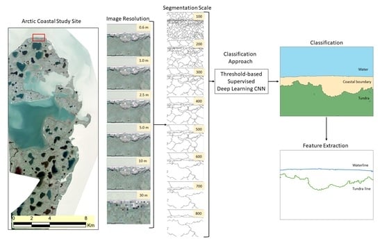
2. Materials and Methods

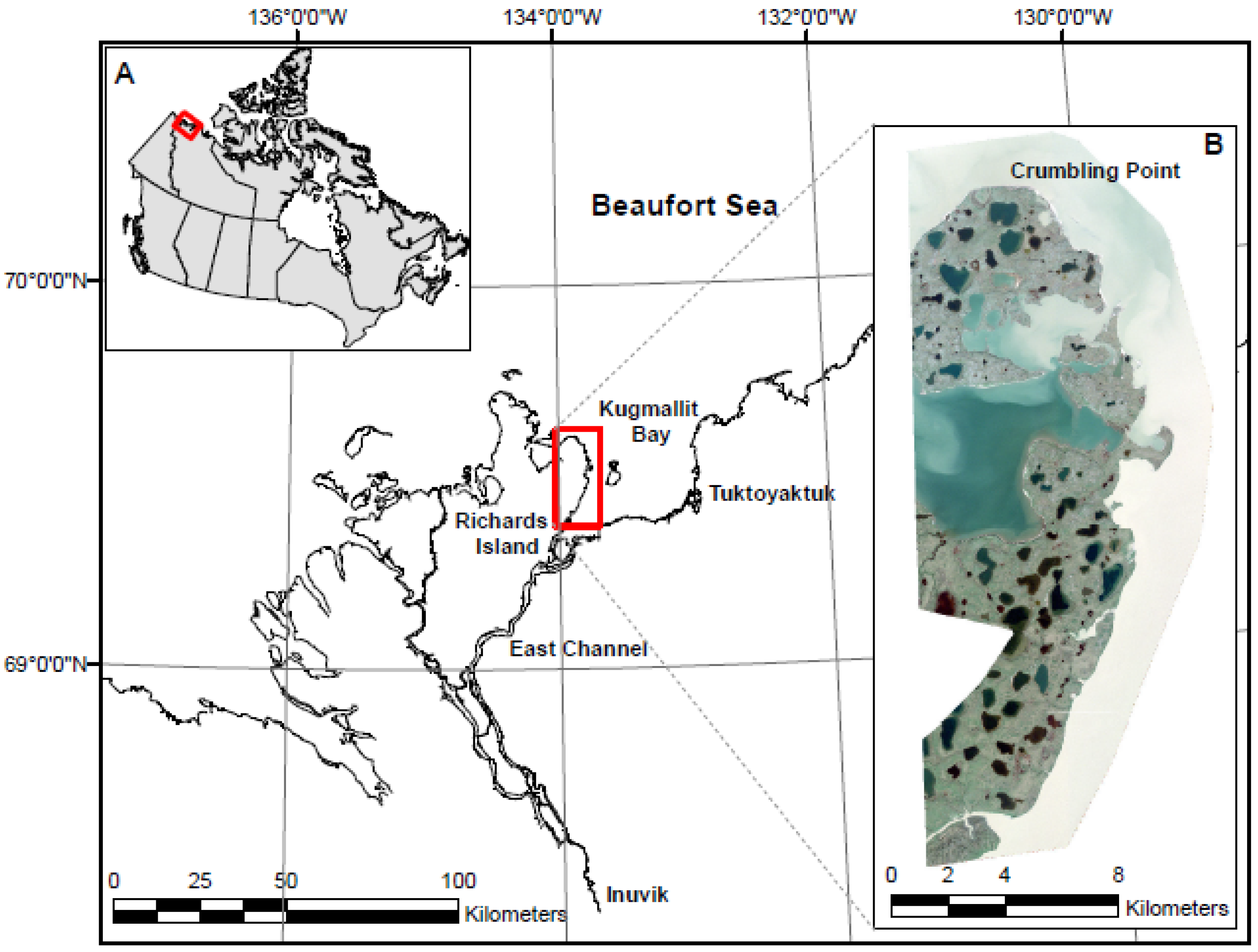
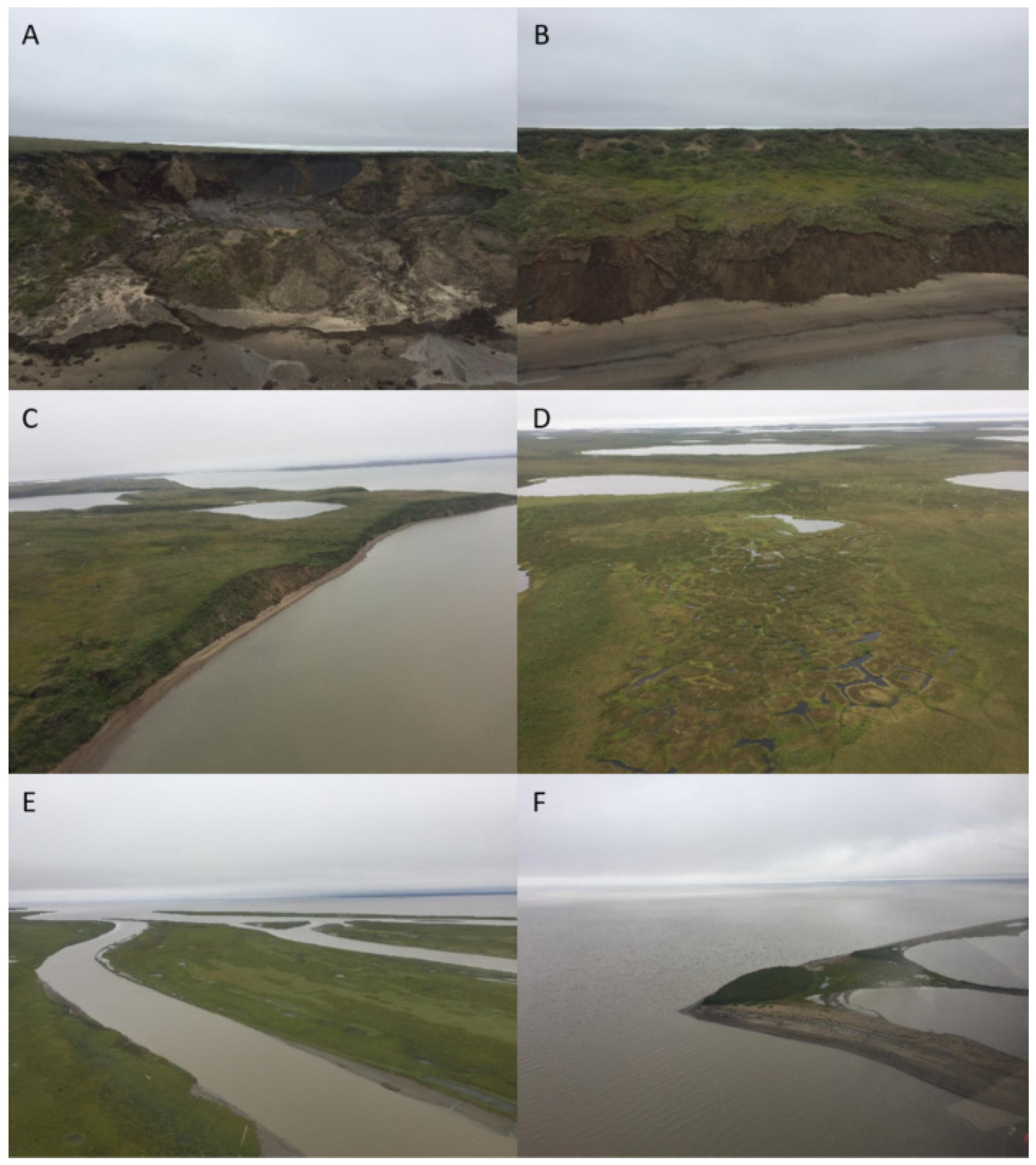
2.1. Study Area

The study site encompasses an approximate area of 210 km² in Beaufort Sea of the western Canadian Arctic in the Northwest Territories (NT) (69°31′17.33″N, 133°52′24.76″W) (Figure 1). The nearest population center, the Hamlet of Tuktoyaktuk, NT, is located 34 km southeast of the study site. The mean annual air temperature recorded at Tuktoyaktuk, NT, between 1981 and 2010 was −10.1 °C with average daily air temperatures of −26.6 °C in January and 11.0 °C in July, with the mean annual air temperature increasing by 3 °C per century during the open water season [50]. In our study site, there is approximately 162 km of ocean-connected coastline with a predominant easterly exposure with a portion that is protected from direct wave action in the form of a bay found in the approximate geographic center of the study site. The northernmost extent of our study site is known as Crumbling Point (69°36′20.08″N, 133°53′37.27″W), which is the location of a 600-m-long polycyclic retrogressive thaw slump with maximum width of 200 m from the shoreline. The polycyclic RTS has a rapidly retreating headwall and experiences substantial coastal cliff erosion [28], which deposits sediments in the near shore zone that are then moved along the coast through longshore transport, creating an 800-m-long sandspit southeast of the RTS.

The area is underlain by continuous permafrost with nearby Richards Island having 600–700 m permafrost thickness [51] and mean annual ground temperatures of −8 to −9 °C [52]. The area is typical of the Tuktoyaktuk Coastlands being spotted with thermokarst lakes, and in some cases susceptible to breaching and subsequent draining from coastal erosion of the non-lithified sediments found throughout the region. The region is typically ice-free from late June to October with changes to the Arctic sea ice regime leading to a lengthening of the open water season [53] resulting in increased open-water fetch for wave generation [54,55].

2.2. Source Data

We used a Pléiades satellite image scene (CNES, Airbus), acquired on 23 July 2018, by the PHR 1B platform, as our primary data source. The scene covered an area of approximately 210 km² and was cloud free. The image was provided as a 0.6m panchromatic band and four 2.4 m multispectral bands (red, green, blue, NIR) in the WGS 1984 geographic coordinate system. A pansharpened dataset was created using the Gram-Schmidt sharpening type with weights of 0.9, 0.75, 0.5, and 0.5 for the red, green, blue, and infrared bands, respectively, resulting in a 0.6 m multispectral image (RGB, NIR) with 16-bit unsigned pixel depth. The image was projected into the NAD 1983 UTM Zone 8N projected coordinate system and resampled based on nearest neighbor into 1, 2.5, 5, 10, and 30 m resolutions using ArcGIS Pro version 2.8.0 (Esri, Redlands, CA, USA).

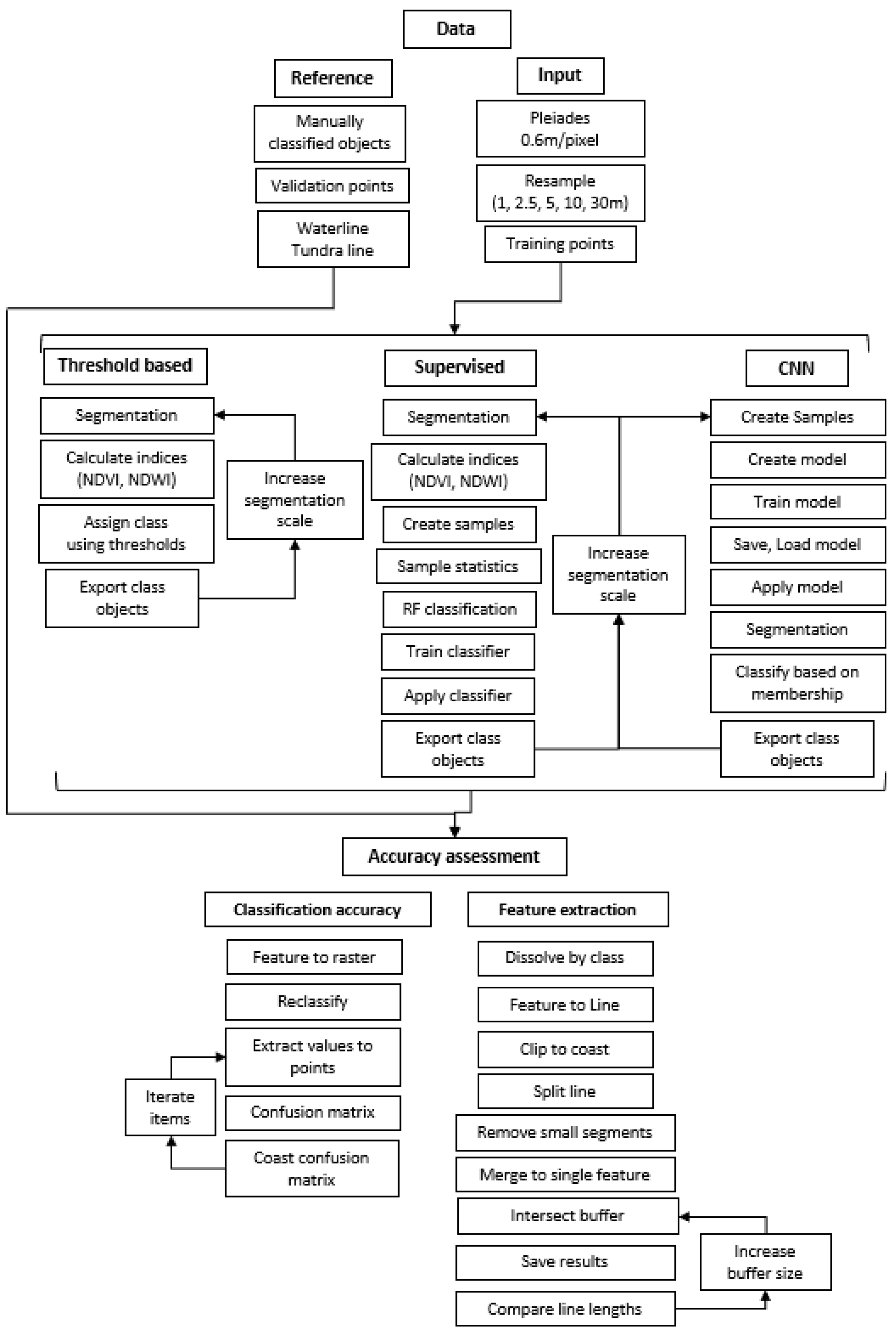
2.3. Classification Approaches

Object-based classifications were conducted using Trimble’s eCognition Developer version 9 software, which enables users to build classification workflows in the form of rule sets from an extensive library of algorithms. Image objects provide the building blocks of our classifications, as opposed to pixels, and were created using the multiresolution segmentation algorithm with equal weighting given to all MS bands. The segmentation parameters of scale, shape, and compactness were determined through iterative testing. The shape and compactness parameters range between 0 and 1 where the shape parameter provides balance between shape and color, while the compactness parameter provides balance between compactness and smoothness [56]. The shape parameter influences the effect of spectral reflectance on the segmentation process and compactness refers to the ratio of border length to area. Therefore, the higher the shape parameter, the lower the influence of color and the higher the compactness parameter, the more compact the object will be [57,58,59,60]. Through iterative testing (trial and error), a shape value of 0.6 and a compactness value of 0.5 were determined to create appropriate objects for our application.

The scale parameter is used to control average image object size [41,42] where a higher value results in bigger objects and a smaller value results in smaller objects. The scale parameter has been considered the primary factor for segmentation in object-based research [43,44] and the determination of the scale parameter depends on factors such as the sensor type, resolution, the purpose of the segmentation, and objects of interest. As a result, we incremented our scale parameter by 100 between 100 and 800 in our threshold-based and supervised classifications to better understand the influence of object size on accuracy. Because objects constitute our building blocks, which should be as large as possible but small enough to provide good object primitives, it was necessary to systematically isolate the scale parameter.

We determined three target classes for this analysis: water, tundra, and coastal boundary zone (Figure 2). The Water class encompasses ocean connected waters and thermokarst lakes. The Tundra class encompasses upland vegetated areas. The coastal boundary zone represents the land area between the water and tundra classes. The coastal boundary zone can be further subdivided into classes of beach, or sand, cliff, retrogressive thaw slumps, and semi-submerged ice wedge polygons but we chose to simplify the classification into a single class.

2.3.1. Threshold-Based Classification

A threshold-based classification workflow was developed in eCognition Developer (Trimble, Sunnyvale, California, United States) (Figure 3) to assign objects into the desired classes of water, tundra, and coastal zone. Using the multiresolution segmentation algorithm, image objects were created, and subsequent indices were calculated for each object.

$$NDVI=\frac{NIR-Red}{NIR+Red}$$

(1)

$$NDWI=\frac{Green-NIR}{Green+NIR}$$

(2)

Using the assign class algorithm, user-defined thresholds were determined and used to classify image objects. Objects with a high NDVI (≥0.3), or presence of vegetation, were assigned to the Tundra class and objects with a high NDWI (≥0.4), or presence of water, were assigned to the Water class. An additional threshold of NDWI ≥ 0.1 and mean digital number of NIR ≤ 300 was used to classify the remainder of the Water class. The remaining unclassified objects were assigned to the coastal boundary zone. Lastly, the export vector layer algorithm was used to export the classified image objects as a polygonal shapefile. The rule set was then applied to a new set of objects created by incrementing the scale parameter. Further, the threshold-based classification was applied to down sampled versions of the satellite scene (1, 2.5, 5, 10, and 30 m) that reflect typical resolutions of satellite imagery products. In total, 48 scenarios were generated to be evaluated in the accuracy assessment.

2.3.2. Supervised Classification

Training samples were created in ArcGIS Pro using the Create Accuracy Assessment Points tool. Forty points were created for each class for a total of 120 training points based on a manual interpretation of the point locations. Image objects were created in the same way as the threshold-based classification where object size was varied by incrementing the scale parameter and iterating through down sampled satellite scenes. From here, we created samples within eCognition from our input vector training samples using the assign class by thematic layer algorithm. Training sample objects were converted to a sample statistics file used to train a random forest (RF) classifier. Sample statistics used were the object mean values and standard deviations for the RGB and NIR input layers. The RF classifier was applied, and classified image objects were exported as a polygonal shapefile to be further assessed using our accuracy assessment workflow.

2.3.3. Deep Learning Classification

We chose to create a convolutional neural network classification using only the highest available image resolutions (0.6 and 1 m/pixel) based on preliminary results of our previous classification approaches, assuming that the highest resolution imagery would provide the highest classification accuracies. A CNN is a deep learning neural network algorithm which is mainly used in image classification. The model receives an image as input and with a user-defined number of hidden layers, output classes are generated. For more information on CNN architecture see [40,41]. Our CNN was implemented using the workflow available in eCognition Developer using the algorithms create, train, and apply CNN which are based on the Google TensorFlow^TM library [61].

A CNN classification rule set (Figure 3) was created in eCognition Developer. First, samples were created by importing a set of 3000 ground truth points, 1000 points per class. Ground truth points were generated using equalized stratified random sampling on a manually classified set of image objects. Sample patches of size 64 × 64 pixels were generated for each ground truth point and rotated through 12 different angles to increase the number of training samples. In total, 36,000 samples were created from the original 3000 ground truth sample points. Next, the CNN was created using 2 hidden layers. The first hidden layer had a kernel size of 5 with 12 feature maps and max pooling set to No. The second hidden layer had a kernel size of 3, 12 feature maps, and max pooling set to No. Sample patches were randomized and used to train the CNN. After saving and loading the model, the CNN model was applied to create heat maps of our desired classes (water, tundra, coastal boundary zone) that represent a probability occurrence for each pixel of our image. Further, image objects were created and classified using a membership function created based on the generated heat maps. At this point, further object-based refinements to the classification can be made but we chose to accept the classification without modification and proceeded to export the classified objects and continue with our accuracy assessment.

2.4. Accuracy Assessment

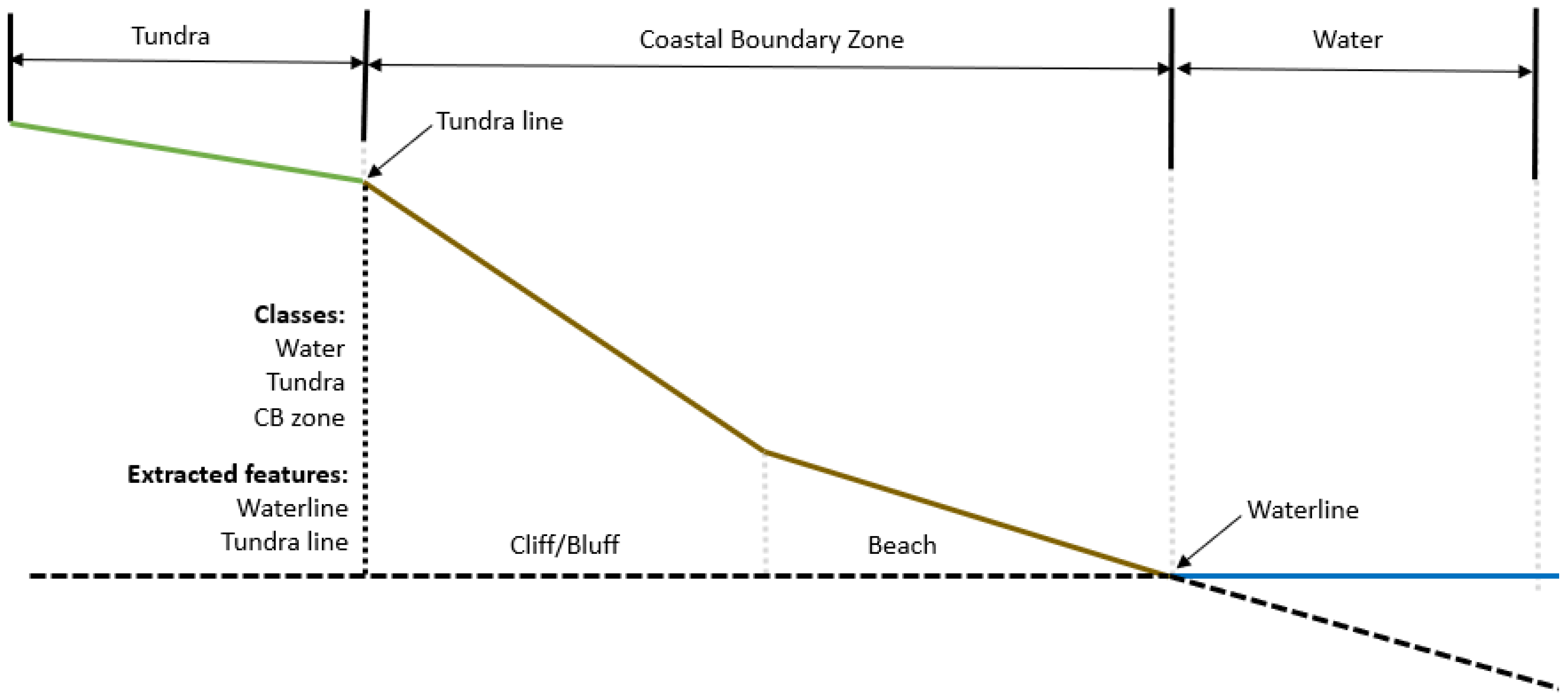
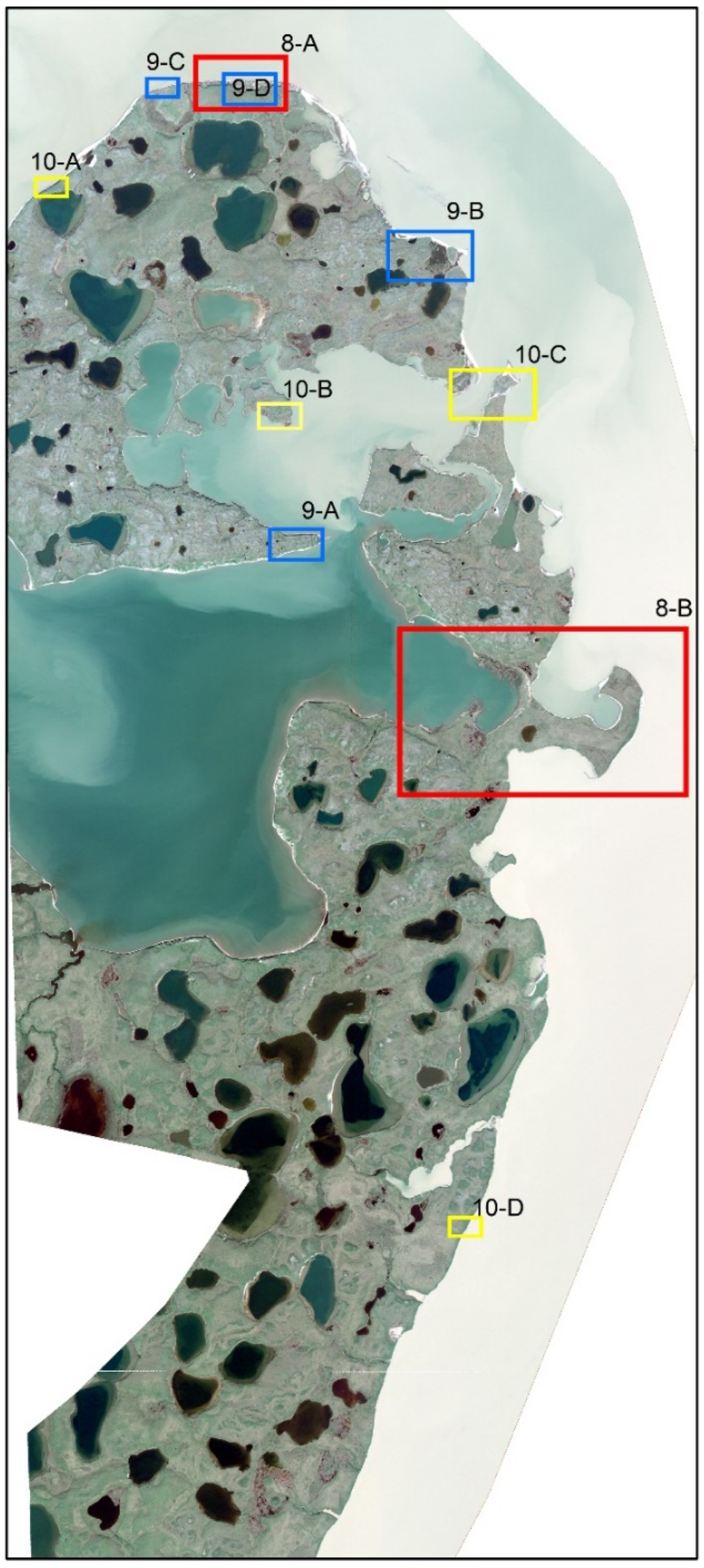
2.4.1. Reference Datasets

A ground truth, or reference, classification was created by manual identification of individual image objects. The interpretation was conducted on image objects derived from the segmentation of the highest resolution scene (0.6 m/pixel) with a scale parameter of 100. This combination of parameters represented the smallest image objects, or building blocks, used in our analysis, and constituted roughly 70,000 image objects. Image objects were assigned to our primary classes of Water, Tundra, and Coastal boundary zone, but an additional class, of Uncertain, was added during this process to assign objects whose class membership were not readily apparent. The 0.6 m/pixel resolution image scene was used as the primary basemap with additional image server basemaps used to help identify the appropriate class of Uncertain objects. In some instances, image objects spanned multiple classes in which case the image object polygons were modified to separate the classes.

A set of 300 validation points (100 per class) were created using equalized stratified random sampling. The set of validation points was verified against the image scene and reference classification and found to be in perfect agreement. A separate set of 300 validation points were created within a 100 m buffer of a generalized coastline using the same approach. This reference point set was used to determine if there is a difference in classification accuracy for a subset of the output classifications.

2.4.2. Confusion Matrices

Confusion matrices were created for each output classification following the steps of Figure 3. The vector-based classifications were converted to raster files using the Assign Class field in ArcGIS Pro, from which a new point file was created by sampling our validation point sets, both the coastal and entire scene, to the classified raster image. The point files, with classified and ground truth fields, were used to compute confusion matrices of our classifications.

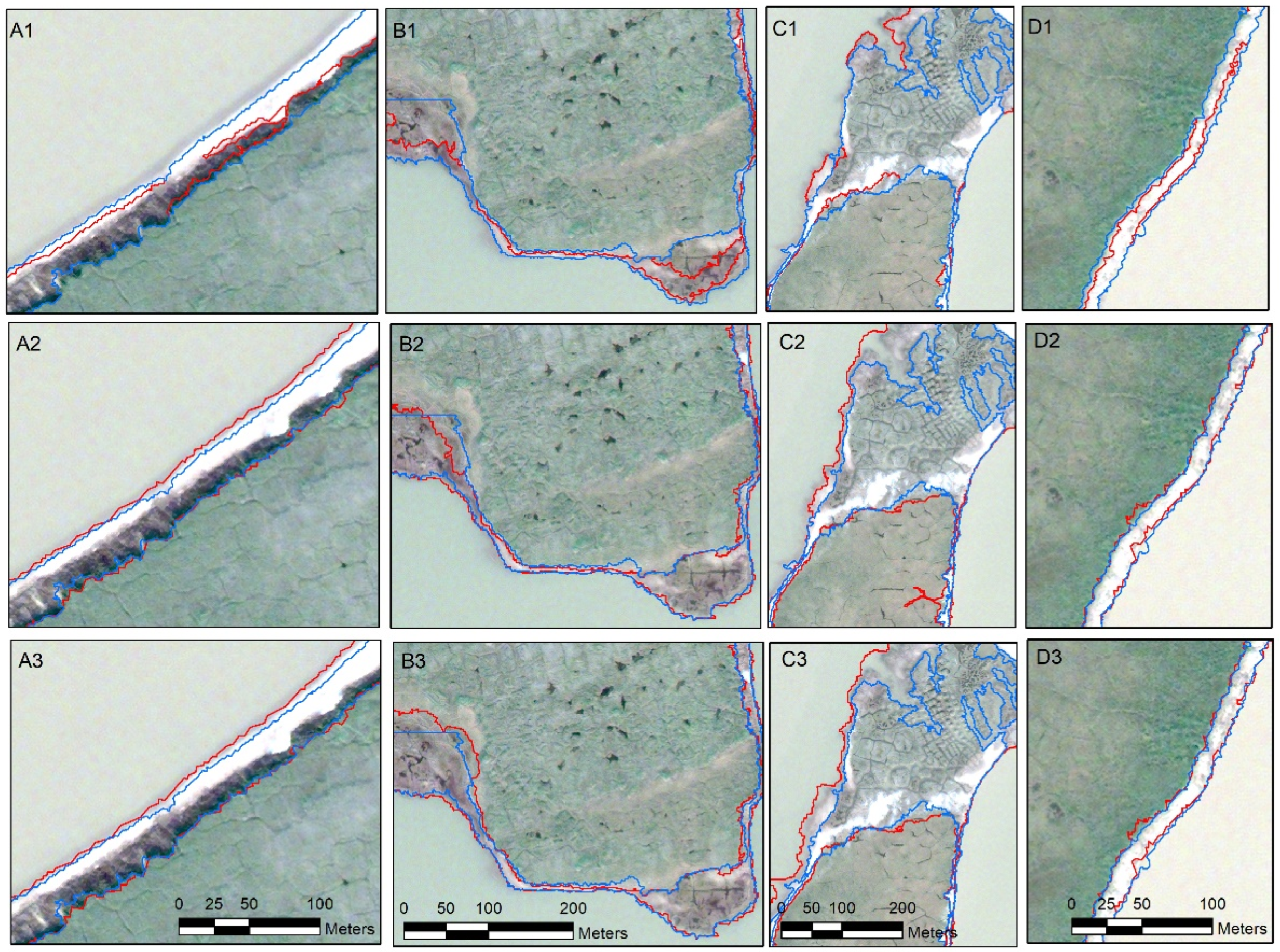
2.4.3. Feature Extraction

Using the vector-based classifications, the waterline and tundra line features were extracted, following the steps in Figure 3, creating two coastal indicator features [62]. These feature lines were evaluated using a buffer analysis [63] with buffers of size 1–10 m at 1 m increments created from reference feature lines. The reference feature lines were extracted from our reference classification using the same methods, which gave a baseline feature length. The extracted coastal indicator features from the classification scenarios were intersected with the set of buffers resulting in a percent of coastal feature lying within each buffer relative to the reference feature lines. Feature extraction from the CNN classifications was only conducted on the 0.6 and 1.0 m/pixel resolution imagery because it was assumed based on preliminary results that the highest resolution imagery would provide the highest feature extraction accuracies.

3. Results

We analyzed a 210 km² satellite scene composed of approximately 75 km² (36%) of water and 135 km² (64%) of land. To investigate the classification and feature extraction accuracies of an object-based approach, we resampled our original dataset of 0.6 m/pixel resolution to 1.0, 2.5, 5, 10, and 30 m/pixel resolution and varied the segmentation scale parameter to alter object size. Because our primary area of interest is the coastal zone, we evaluated our classification accuracies for the entire scene as well as a 100 m buffered area from a generalized coastline to determine if there was a marked difference. Further, feature extraction was limited to the waterline and tundra lines, or vegetation line, of the coastal zone as the primary goal was to investigate the ability of an object-based approach to accurately identify coastal indicators as opposed to similar scene features such as the land–water interface of thermokarst lakes.

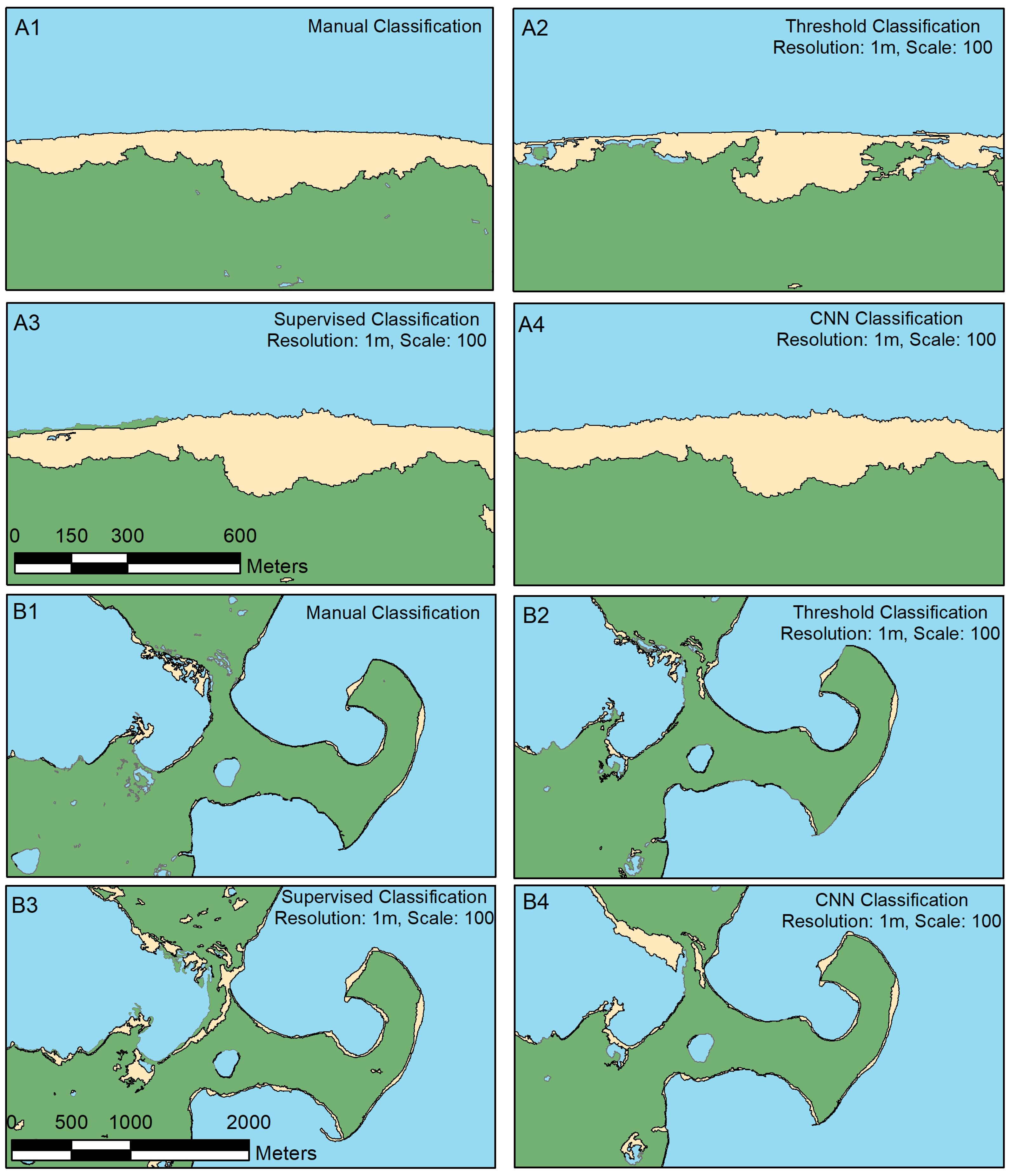
3.1. Classification Accuracy

3.1.1. Threshold-Based Classification

There was a consistent improvement in classification accuracy by several percentage points when restricting the area of evaluation to the 200 m coastal zone (

Table 1. Threshold classification accuracies generated from a confusion matrix. Six image resolutions (rows) and eight segmentation scales (columns) are presented as percentages with averages for individual image resolutions across segmentation scales. Kappa values given. Accuracy assessments were conducted for the entire scene (upper value) and a 200 m coastal zone (lower value).

	Resolution	100	200	300	400	500	600	700	800	Average	Kappa
Scale Segmentation (m)
0.6	Entire Scene	83	83	83	84	85	84	84	84	84	0.75–0.78
	Coastal Subset	84	87	87	89	88	89	88	90	88	0.76–0.85
1	Entire Scene	83	86	87	85	84	83	85	85	85	0.75–0.81
	Coastal Subset	86	87	89	89	87	87	88	88	88	0.79–0.84
2.5	Entire Scene	85	85	86	86	87	86	82	82	85	0.73–0.81
	Coastal Subset	87	87	88	88	87	86	85	85	87	0.78–0.82
5	Entire Scene	85	84	81	78	75	75	75	74	78	0.61–0.78
	Coastal Subset	87	88	88	77	76	77	75	75	80	0.63–0.82
10	Entire Scene	81	76	69	67	65	30	21	21	54	0.25–0.71
	Coastal Subset	80	75	68	62	60	60	64	64	67	0.41–0.71
30	Entire Scene	69	61	62	63	62	62	62	50	61	0.24–0.54
	Coastal Subset	66	63	61	61	56	56	56	41	58	0.12–0.49

). Overall, for image resolutions of 0.6, 1.0, and 2.5 m/pixel (very high resolution), the classification accuracies were consistent across all segmentation scales whereas image resolutions of 5, 10, and 30 m/pixel (high resolution) were found to have a steady decrease in classification accuracy as the segmentation scale parameter increased. In addition, the classification accuracies of the very high resolution datasets were considerably higher than that of the high resolution datasets. Classification accuracies ranged between 83 and 90% using the very high resolution datasets and 21 and 85% for high resolution datasets; however, when using a small segmentation scale (100–300) on the 5 m/pixel resolution dataset, there were comparable accuracies to the very high resolution datasets. Similar trends existed for the kappa coefficient, a measure of model accuracy relative to a random classifier used to compare between classifiers, where there was a small, consistent, increase between the overall scene and when restricting to the coastal zone. Beyond a resolution of 5 m/pixel at segmentation scale larger than 300, the kappa coefficients decrease dramatically.

The number of objects created through the multiresolution segmentation process was a function of image resolution and segmentation scale parameter where more objects are created for higher resolution images with small scale parameters. However, the number of original image objects created did not directly impact classification results for the very high resolution datasets. For example, in the 1 m/pixel image scenario, there were over 25,000 image objects created with a 100-scale parameter and 692 image objects created with an 800-scale parameter, but the classification accuracies and kappa coefficients varied minimally. In contrast, far fewer objects were created on the medium resolution datasets particularly at large segmentation scale resulting in a dramatic decrease in classification accuracies especially on the 10 and 30 m/pixel where fewer than 100 objects were created in 12 of the 16 scenarios.

3.1.2. Supervised Classification

In the supervised classification scenarios, there was minimal difference between classification accuracies when assessing over the entire scene or restricting to the coastal zone. The classification accuracies using a supervised classification approach were marginally to substantially better in almost all cases compared to the threshold-based approach. However, there was more variability between scales of segmentation in the supervised classification accuracies for a given resolution including notably low accuracies for the highest resolution—smallest segmentation scale. For the very high resolution datasets, there was an at least 8% difference between the highest and lowest achieved accuracies within a given data resolution with a maximum range of 28 points for the highest resolution dataset (0.6 m/pixel). The medium resolution datasets saw a general downward trend in classification accuracies with increasing segmentation scale following the pattern observed in the threshold-based classification where too few objects are created to produce an accurate classification. The best overall classification accuracy was achieved using resolutions of 1 and 2.5 m/pixel with average accuracies of 88 and 86% (

Table 2. Supervised classifications were generated using 120 samples (40 per class) and assessed using 200 validations points across the entire scene (upper value) and a separated 200 validations points in the coastal zone (lower value). A total of 48 classification scenarios were generated by modifying image resolution and segmentation scale.

	Resolution	100	200	300	400	500	600	700	800	Average	Kappa
Scale Segmentation (m)
0.6	Entire Scene	62	77	81	90	76	88	88	86	81	0.43–0.83
	Coastal Subset	69	85	81	90	76	90	89	88	84	0.54–0.85
1	Entire Scene	91	90	88	88	85	94	86	85	88	0.77–0.86
	Coastal Subset	90	90	90	90	86	87	87	87	88	0.8–0.86
2.5	Entire Scene	90	88	88	87	88	89	85	82	87	0.73–0.84
	Coastal Subset	91	87	87	86	86	86	84	83	86	0.77–0.87
5	Entire Scene	85	84	84	80	79	76	75	77	80	0.62–0.78
	Coastal Subset	86	87	85	79	78	77	75	75	80	0.62–0.81
10	Entire Scene	80	78	74	70	68	62	63	63	70	0.43–0.7
	Coastal Subset	81	77	71	65	63	60	64	64	68	0.4–0.72
30	Entire Scene	71	61	62	54	62	62	62	50	61	0.24–0.56
	Coastal Subset	66	63	61	53	56	56	56	41	57	0.12–0.5

), respectively, in the coastal zone. Kappa coefficients were highest among the 1m/pixel resolution dataset up to a segmentation scale parameter of 400. High kappa coefficients were also produced for the 2.5 m/pixel resolution dataset at a segmentation scale parameter of 100 with reduced but consistent values thereafter. Conversely, at the highest resolution available (0.6 m/pixel), classification accuracies and kappa coefficients were relatively low at segmentation scales of 100, 200, 300, and 500.

3.1.3. CNN

Images (0.6 and 1 m/pixel resolutions) classified using deep learning convolutional neural networks (CNN) provided the highest classification accuracies and kappa coefficients. The CNN classifier achieved an average overall accuracy of 93% and a kappa coefficient up to 0.93 on the 0.6 m/pixel resolution image. On the 1m/pixel resolution image, the CNN classifier achieved an average overall accuracy of 91% with a kappa coefficient up to 0.92. Interestingly, the overall scene was classified to a higher accuracy than the coastal zone representing a departure from the trend observed in threshold- and supervised-based classifications. The single highest accuracies observed were when a small segmentation scale (100) was used with a classification accuracy of 95% and 0.93 kappa coefficient.

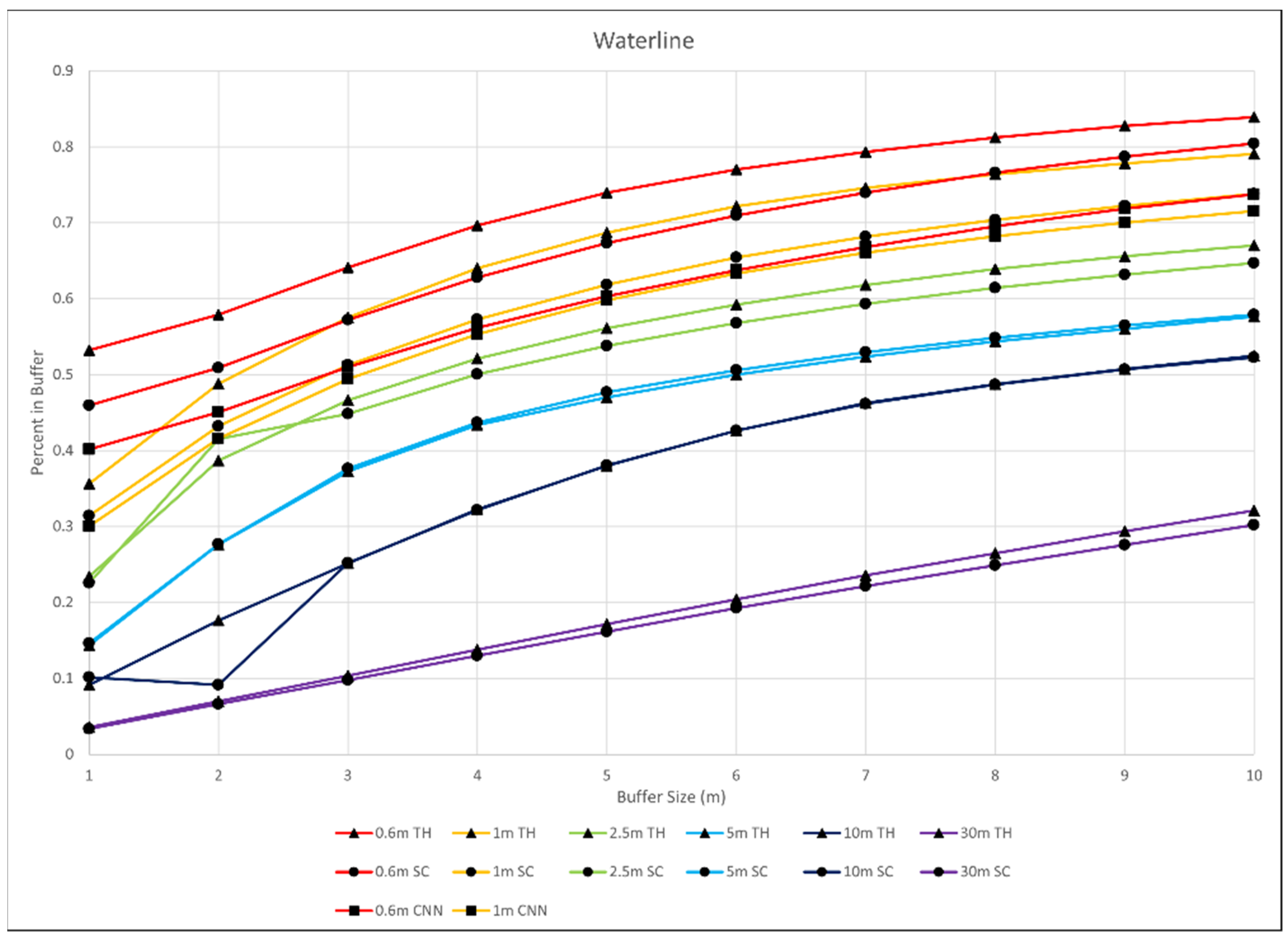
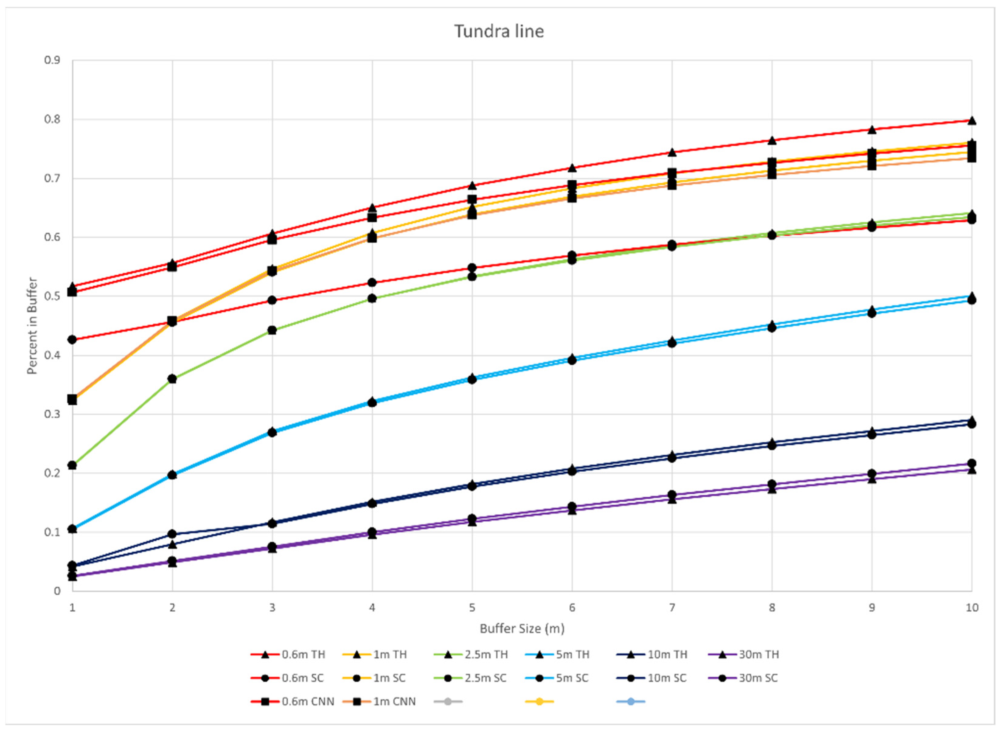
3.2. Feature Extraction

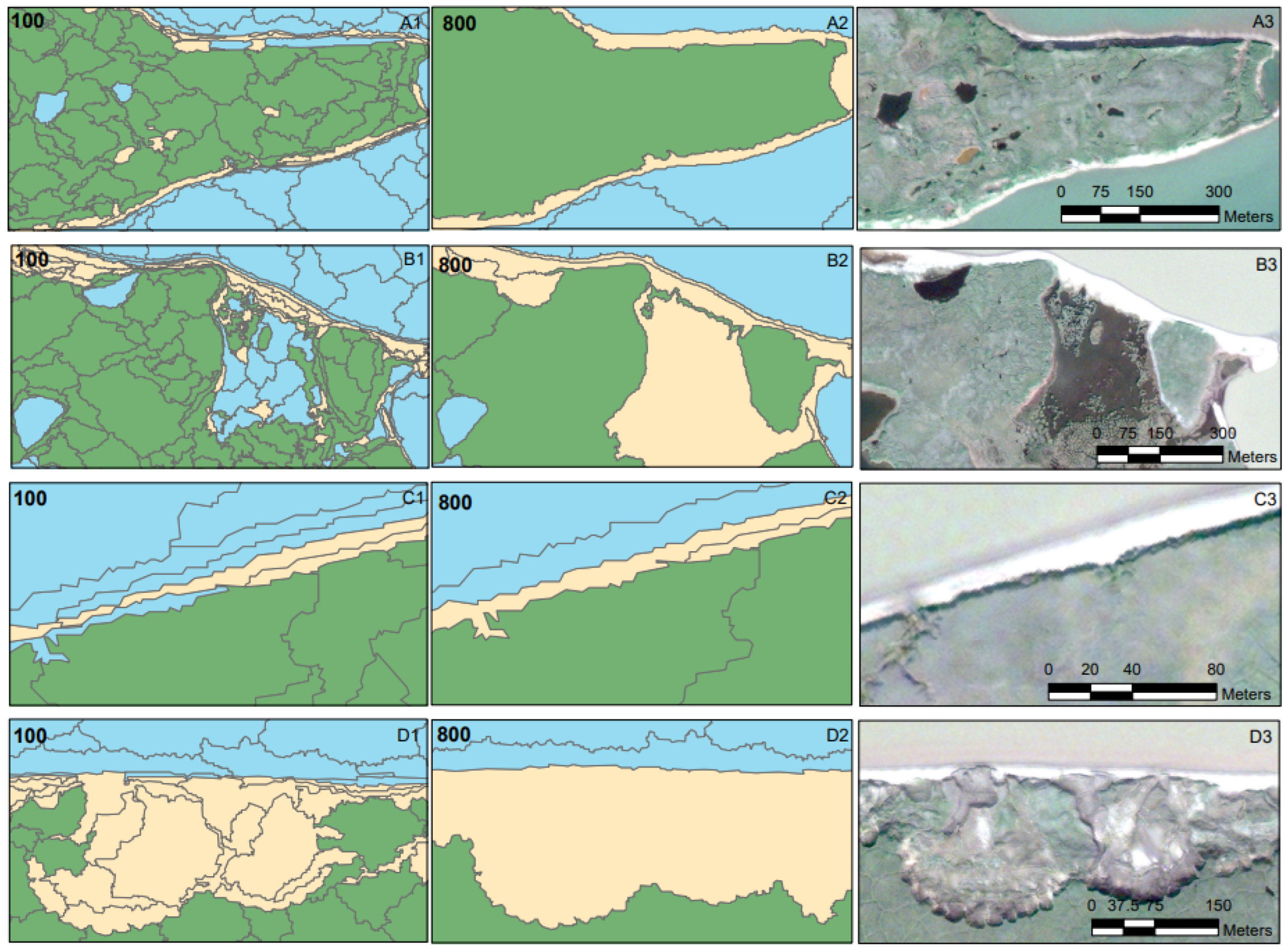
3.2.1. Threshold-Based Classification

Segmentation scale and image resolution (i.e., object size) played a critical factor in the percentage of line features within a given buffer size around the reference feature lines. For nearly all resolution scenarios, the percentage of coastal feature, relative to reference, decreased with increasing segmentation scale. Similarly, the percentage within a given buffer size decreased with increasing image resolution (Figure 4 and Figure 5). As a result, the best results were achieved on very high resolution datasets with small segmentation scale parameters (Figure 4 and Figure 5). At a 1m buffer size, across all segmentation scales, there was an approximately 20% improvement between the 1m/pixel resolution image and the 0.6 m/pixel resolution image.

The accuracy was also dependent on the coastal indicator. There was a consistent bias where the waterline was extracted more accurately than the tundra line, particularly in very high resolution images. In the 0.6 m/pixel image, with a scale parameter of 100, the waterline showed a 10% higher accuracy over the tundra line across all buffer sizes. In the best case (0.6 m/pixel image, 100 scale), the waterline was within 1m of the reference waterline 60% of the time and the tundra line was within 1 m of the reference tundra line 50% of the time. Increasing the buffer size to 5 m, the percentages increase to 81 and 70% for the waterline and tundra lines, respectively. Finally, 92% of the waterline and 83% of the tundra line were within 10m of the reference feature lines.

3.2.2. Supervised Classification

The trends of increasing pixel size and segmentation scale leading to reduced feature extraction accuracy were maintained for high resolution scenarios but there was more variability among the very high resolution datasets. In many cases, the tundra line was close if not better than the waterline and increasing the segmentation scale led to a slight improvement in results. However, in the 0.6 m/pixel resolution scenario, there tended to be large differences between the waterline and tundra lines for some segmentation scales whereas other segmentation scales exhibited more typical behavior. For example, at a 100-segmentation scale, the 10 m buffer captured 98% of the waterline but only 40% of the tundra line, and at an 800-segmentation scale, the 10 m buffer captured 74% of the waterline and 79% of the tundra line. Generally, for a given resolution and segmentation scale, the features extracted from the image objects through supervised classification did not perform as well as the threshold-based approach but tended not to have a bias towards the waterline. In addition, in the 0.6 m/pixel image scenario, which provided the best results in the threshold-based approach, did not provide consistent results. Therefore, the best results were achieved on the 1 m/pixel resolution image with a scale parameter of 100 corresponding to 32% of the waterline and 33% of the tundra line falling within 1 m of the reference feature lines. The 5 m buffer captured 64% of the waterline and 66% of the buffer line while the 10 m buffer captured 77% of the waterline and 78% of the tundra line. The tundra lines are comparable to the threshold-based approach while the waterline was several percentage points lower on average. Further, the best of the supervised approach was considerably less accurate than the best of the threshold-based approach.

3.2.3. CNN

For the CNN classifier scenarios (0.6, 1 m/pixel resolution, all segmentation scales), feature extraction was over 10% more accurate on the 0.6 m/pixel image than the 1 m/pixel image. Unlike the previous methods, a smaller segmentation scale did not lead to an increase in feature extraction accuracy using the CNN classifier method with the best results achieved with a segmentation scale of 600. Further, the tundra line was extracted more than 10% more accurately than the waterline. In the best case, the waterline was extracted to within 1m of the reference line 42% of the time while the tundra line was extracted to within 1m of the reference line 54% of the time. Increasing the buffer size to 5 m captured 62% of the waterline and 67% of the tundra line. At a 10 m buffer size, 75% of the waterline and 77% of the tundra line were captured using our methods.

4. Discussion

The presented methodology provides a new approach to studying Arctic coastal erosion that is highly adaptable and integrates well into automated workflows. Through object-based image segmentation, very high resolution satellite imagery was classified with high accuracy. Subsequently, two important coastal indicator features, the waterline and tundra line, were extracted with encouraging results. We attribute some of the inconsistencies to the complexity and variability of the coastal zone (Figure 6), which is a frequent issue described in the coastal erosion literature [64].

Figure 7 provides an overview of the study area with the extent indicators for areas of interest highlighted in Figure 8, Figure 9 and Figure 10. High classification accuracies were achieved, particularly for common very high image resolutions, across all three tested classification approaches (Figure 8, Table 1, Table 2 and

Table 3. CNN classifications were generated for the highest resolution images available (0.6 and 1.0 m/pixel) across the eight segmentation scales. Classification accuracies were evaluated using the same approach as threshold and supervised classifications for the entire scene (upper value) and coastal zone (lower value). Each confusion matrix was based on 200 validation points. Of all classification approaches, the deep learning CNN classifier resulted in the highest accuracy and kappa coefficients.

	Resolution	100	200	300	400	500	600	700	800	Average	Kappa
Scale Segmentation (m)
0.6	Entire Scene	95	94	95	94	92	92	93	93	93	0.88–0.93
	Coastal Subset	91	91	90	91	91	91	90	89	91	0.84–0.87
1	Entire Scene	95	93	93	91	89	88	88	88	91	0.82–0.92
	Coastal Subset	88	88	89	89	88	88	88	88	88	0.82–0.83

), with the deep learning CNN providing the best classifications. In all cases, the tundra and water classes were classified with very high accuracy, but the overall accuracy was impacted by the challenges in identifying the coastal boundary zone class, which was commonly misclassified as tundra. Further, we found there to be a slight increase, in many cases, in classification accuracy when the assessment area was restricted to a 200-m-wide area of the coastal zone. Due to the thermokarst lake features covering the landscape, there is an increased number of land–water transitional zones, which increases the prevalence of the coastal boundary zone class, resulting in more occurrences of model confusion. Interestingly, the deep learning CNN approach saw a small decrease in accuracy for the coastal zone assessment area, suggesting this method was better able to classify thermokarst lake transitional zones. The difficulty of classifying the coastal boundary zone is exemplified in B panels of Figure 8, where in low lying transitional areas, irregular objects are produced due to local variability and introduce subjectivity in creating reference and training data. The class transition zone between the Water class and the Coastal boundary class can also be impacted by wave breaking [65]. We were able to avoid misclassifications by using a low cloud cover scene, but it was common for shadows caused by steep north facing slopes to be misclassified as the Water class, particularly in the threshold-based classification (Figure 8). The polycyclic retrogressive thaw slump (Figure 8(A1–A4) and Figure 9(D1–D3)), which are unique coastal processes in the Arctic, at Crumbling Point was particularly well identified using DL and supervised classifications suggesting the importance of high-quality training datasets. However, due to the presence of vegetation in stabilized areas, the RTS becomes highly ambiguous and hardly discernable [29], resulting in the threshold-based classification to identify unvegetated areas of the slump, suggesting that a hierarchical approach may be able to distinguish between active and inactive retrogressive thaw slumps.

In segmentation-based approaches, the segmentation depends on the shape, compactness, and scale parameters, which will differ based on imaging sensor, resolution, and application [31] and is typically a practice of trial-and-error. We fixed the shape and compactness parameters at 0.6 and 0.5, respectively, but tested eight different segmentation scales (100, 200, 300, 400, 500, 600, 700, and 800) to determine the most appropriate image-object size for Arctic coastal classifications. From Figure 9, we see that a small segmentation scale (100) leads to more detail and therefore more variability, but a large segmentation scale (800) gives a more generalized view that potentially misses key information. Broadly, the segmentation scale did not impact classification results on very high resolution imagery (0.6, 1, and 2.5 m) but on high resolution imagery (5, 10, and 30 m) having a small segmentation parameter (i.e., smaller/more objects) led to higher classification accuracies. In contrast, feature extraction accuracy increased with decreasing segmentation scale because the coastal zone was made up of more image objects leading to more precision in the location of boundaries between classes. However, small objects, particularly in class transition zones, can be misclassified due slope shadows (Figure 9(A1–A3),(C1–C3)), landscape complexity (Figure 9(B1–B3)), or sediment mixing (Figure 9(D1–D3)). Sediment mixing was problematic in identifying the waterline along actively eroding coastal sections and therefore particularly pronounced in the nearshore zone of Crumbling Point, where large amounts of sediment in the waters led to model confusion. Along straight coastal stretches with well-defined beach and cliff features, long linear segments (Figure 9(C1,C2)) are created where over segmentation (Figure 9(C1)) leads to misclassification but under segmentation (Figure 9(C2)) can lead to a loss in precision of the boundary lines.

Four sample locations of feature extraction are shown in Figure 10. Blue lines represent the reference waterline and tundra lines, and red lines represent extracted features. A and D columns show a high and low coastal bluff coastal type, respectively, and highlight areas of effective feature extraction where there is near exact agreement, in many cases, between datasets and the majority within 1m accuracy. Conversely, B and C columns of Figure 10 highlight sample regions where the waterline and tundra line extraction can fall outside an acceptable range where the tundra line is particularly subjective in column B and the waterline in column C. However, because these environments are not actively eroding, they are not likely to contribute to significant coastal land loss or contribute to release of organic carbon into the ocean.

Overall, feature extraction derived from object-based classifications was effective along coastal types with clear boundary lines but proved less effective along coasts with low-centered ice-wedge polygon networks, intertidal zones, and low plain tundra where there is also uncertainty in the reference dataset due to coastal interpretation. For studies measuring coastal bluff and cliff erosion [2,3,18,47], our methods can be effectively applied. Jones et al. [21] removed areas without exposed coastal bluffs from their analysis, further suggesting the applicability of our methods since our buffering technique identifies areas that are indicative of non-eroding coastlines, which can be left out of the analysis.

Figure 4 and Figure 5 presented small differences depending on the classification approach, which is encouraging since very high resolution imagery has become standard for Arctic coastal erosion studies [18,25,48,49]. We see a particularly good fit for our methods to integrate with a novel approach introduced by Lim et al. [66] that derives very high resolution imagery through structure-from-motion photogrammetry from imagery capture by helicopter for Arctic coastal reconstruction introduced for measurement of wide-scale storm impacts. Our contribution of identifying multiple coastal features is well suited for modeling complex coastal processes and environmental forcing factors [18,50].

We suggest that, at minimum, our methods can be adopted to delineate coastal features in the Arctic along coastal stretches with well-defined boundaries and by augmenting with manual interpretation in areas with fuzzy boundaries, greatly improving efficiency. Further, the creation of image objects through segmentation provides the necessary linear features, making the manual interpretation process more streamlined. Our three methods of image-object classification, threshold-based, supervised, and deep learning produced very similar results at all resolutions and segmentation scales; however, each requires method specific intervention of expert knowledge that has implications for widespread application. The threshold values must be determined which may vary depending on satellite scene but was effective at separating water and tundra land cover types. Encouragingly, a study by Abdelhady et al. [65] introduced an automated way to determine threshold values in identifying the waterline along a temperate coastal environment. The supervised and deep learning techniques require high-quality training datasets which must be generated by the user and will determine the quality of the classification. Significantly more training samples are required for deep learning (1000 s vs. 10 s per class) and considerably more computation time and storage. Classifications based on training samples present opportunities to create more information-rich classifications, and potential applications, by introducing more classes and potentially dealing directly with problem areas by classifying the coastal zone into subclasses. Similar work by Nitze et al. [29], where a deep learning, segmentation-based approach for mapping retrogressive thaw slumps further recommends the importance of pan-Arctic training data for DL-based applications. We believe a deep learning approach augmented with expert knowledge refinements, such as thresholding, would ultimately provide the most robust approach for wider application.

5. Conclusions

We tested three object-based classification approaches, threshold-based, supervised, and a deep learning CNN, to understand their applicability to be integrated into an automated workflow for wide-scale measurement and monitoring of Arctic coastal change. First, we assessed the accuracy of a classified satellite scene, representing a typical coastal area of the Western Canadian Arctic, at multiple resolutions and varying the segmentation scale to create image-objects of multiple sizes. Next, based on the classifications, we extracted waterline and tundra line coastal indicator features, which are linear features typically used to measure coastal erosion, and evaluated against manually interpreted reference features. We achieved classification accuracies up to 95% on very high resolution versions (0.6, 1, 2.5 m/pixel) of the satellite scene with the deep learning CNN classifier consistently providing the highest accuracies. The image resolution and segmentation scale were influential in feature extraction accuracy which tended to favor the smallest pixel and segmentation size because of the increased precision. The waterline and tundra lines were extracted with similar accuracy, but the waterline tended to slightly outperform the tundra line, likely due to their relative complexities.

Our study represents an important contribution to wide-scale, high temporal, Arctic coastal monitoring through the development of automated workflows. A fully automated approach may be difficult to ever achieve but we have shown at least a 50% reduction in labor-intensive manual processing that furthers eases the burden of manual intervention by providing homogenous vector objects. We generated multiple coastal features from very high resolution imagery which we believe should become standard among Arctic coastal erosion studies to provide study-to-study comparisons but also to ensure that the most appropriate feature is used for a given application. For example, when quantifying volumetric erosion to estimate greenhouse gas release from permafrost coasts, the changes to the tundra line of actively eroding coasts would be more appropriate while the waterline may be sufficient for long-term marine transgression. Our models struggled along complex coastal types such as low plains and wetlands without well-defined boundaries but performed very well along coastal types with well-defined boundaries. We anticipate that further development of a deep learning approach and introduction of additional coastal boundary zone subclasses will lead to improvements along challenging coastal types, particularly with advancements in high-quality training datasets. Additional investigations should look to apply segmentation-based approaches across extensive areas of interest, over multiple time steps, and the use of ArcticDEM [67] to better understand and quantify the volumetric erosion of Arctic coasts and the local and global implications. Finally, while we were specifically interested in coastal classification and feature extraction accuracy to better understand Arctic coastal dynamics and the potential impacts and drivers of climate change, but the high accuracy achieved across the entire study site suggests that our approach could be adapted to a range of applications specific to the Arctic that require widespread monitoring such as the identification and evolution of retrogressive thaw slumps, thermokarst lakes, and ice-wedge polygon networks.

References

1. Jones, B.M.; Irrgang, A.M.; Farquharson, L.M.; Lantuit, H.; Whalen, D.; Ogorodov, S.; Grigoriev, M.; Tweedie, C.; Gibbs, A.E.; Strzelecki, M.C.; et al. Coastal Permafrost Erosion; Atmospheric Administration: Washington, DC, USA, 2020; pp. 1–10. [CrossRef]
2. Günther, F.; Overduin, P.P.; Yakshina, I.A.; Opel, T.; Baranskaya, A.V.; Grigoriev, M.N. Observing Muostakh Disappear: Permafrost Thaw Subsidence and Erosion of a Ground-Ice-Rich Island in Response to Arctic Summer Warming and Sea Ice Reduction. Cryosphere 2015, 9, 151–178. [Google Scholar] [CrossRef] [Green Version]
3. Günther, F.; Overduin, P.P.; Sandakov, A.V.; Grosse, G.; Grigoriev, M.N. Short- and Long-Term Thermo-Erosion of Ice-Rich Permafrost Coasts in the Laptev Sea Region. Biogeosciences 2013, 10, 4297–4318. [Google Scholar] [CrossRef] [Green Version]
4. Jones, B.M.; Arp, C.D.; Jorgenson, M.T.; Hinkel, K.M.; Schmutz, J.A.; Flint, P.L. Increase in the Rate and Uniformity of Coastline Erosion in Arctic Alaska. Geophys. Res. Lett. 2009, 36, 1–5. [Google Scholar] [CrossRef]
5. Lantuit, H.; Pollard, W.H. Fifty Years of Coastal Erosion and Retrogressive Thaw Slump Activity on Herschel Island, Southern Beaufort Sea, Yukon Territory, Canada. Geomorphology 2008, 25, 84–112. [Google Scholar] [CrossRef]
6. Lantuit, H.; Overduin, P.P.; Couture, N.; Wetterich, S.; Aré, F.; Atkinson, D.; Brown, J.; Cherkashov, G.; Drozdov, D.; Donald Forbes, L.; et al. The Arctic Coastal Dynamics Database: A New Classification Scheme and Statistics on Arctic Permafrost Coastlines. Estuaries Coasts 2012, 35, 383–400. [Google Scholar] [CrossRef] [Green Version]
7. Perovich, D.; Light, B. Sunlight, Sea Ice, and the Ice Albedo Feedback in a Changing Arctic Sea Ice Cover; LONG-TERM GOALS; Atmospheric Administration: Washington, DC, USA, 2016.
8. Steele, M.; Dickinson, S. The Phenology of Arctic Ocean Surface Warming. J. Geophys. Res. Ocean. 2016, 121, 6847–6861. [Google Scholar] [CrossRef]
9. Richter-Menge, J. Arctic Report Card; Climate.gov: New York, NY, USA, 2011.
10. Smith, S.L.; Romanovsky, V.E.; Lewkowicz, A.G.; Burn, C.R.; Allard, M.; Clow, G.D.; Yoshikawa, K.; Throop, J. Thermal State of Permafrost in North America: A Contribution to the International Polar Year. Permafr. Periglac. Process. 2010, 21, 117–135. [Google Scholar] [CrossRef] [Green Version]
11. Romanovsky, V.E.; Smith, S.L.; Christiansen, H.H. Permafrost Thermal State in the Polar Northern Hemisphere during the International Polar Year 2007–2009: A Synthesis. Permafr. Periglac. Process. 2010, 21, 106–116. [Google Scholar] [CrossRef] [Green Version]
12. Lim, M.; Whalen, D.; Martin, J.; Mann, P.J.; Hayes, S.; Fraser, P.; Berry, H.B.; Ouellette, D. Massive Ice Control on Permafrost Coast Erosion and Sensitivity. Geophys. Res. Lett. 2020, 47, e2020GL087917. [Google Scholar] [CrossRef]
13. Vermaire, J.C.; Pisaric, M.F.J.; Thienpont, J.R.; Courtney Mustaphi, C.J.; Kokelj, S.V.; Smol, J.P. Arctic Climate Warming and Sea Ice Declines Lead to Increased Storm Surge Activity. Geophys. Res. Lett. 2013, 40, 1386–1390. [Google Scholar] [CrossRef]
14. Farquharson, L.M.; Mann, D.H.; Swanson, D.K.; Jones, B.M.; Buzard, R.M.; Jordan, J.W. Temporal and Spatial Variability in Coastline Response to Declining Sea-Ice in Northwest Alaska. Mar. Geol. 2018, 404, 71–83. [Google Scholar] [CrossRef]
15. Fritz, M.; Vonk, J.E.; Lantuit, H. Collapsing Arctic Coastlines. Nat. Clim. Chang. 2017, 7, 6–7. [Google Scholar] [CrossRef] [Green Version]
16. Tanski, G.; Wagner, D.; Knoblauch, C.; Fritz, M.; Sachs, T.; Lantuit, H. Rapid CO2 Release from Eroding Permafrost in Seawater. Geophys. Res. Lett. 2019, 46, 11244–11252. [Google Scholar] [CrossRef] [Green Version]
17. Irrgang, A.M.; Lantuit, H.; Manson, G.K.; Günther, F.; Grosse, G.; Overduin, P.P. Variability in Rates of Coastal Change Along the Yukon Coast, 1951 to 2015. J. Geophys. Res. Earth Surf. 2018, 123, 779–800. [Google Scholar] [CrossRef] [Green Version]
18. O’Rourke, M.J.E. Archaeological Site Vulnerability Modelling: The Influence of High Impact Storm Events on Models of Shoreline Erosion in the Western Canadian Arctic. Open Archaeol. 2017, 3, 1–16. [Google Scholar] [CrossRef]
19. Gens, R. Remote Sensing of Coastlines: Detection, Extraction and Monitoring. Int. J. Remote Sens. 2010, 31, 1819–1836. [Google Scholar] [CrossRef]
20. Sankar, R.D.; Murray, M.S.; Wells, P. Decadal Scale Patterns of Shoreline Variability in Paulatuk, N.W.T, Canada. Polar Geogr. 2019, 42, 196–213. [Google Scholar] [CrossRef]
21. Jones, B.M.; Farquharson, L.M.; Baughman, C.A.; Buzard, R.M.; Arp, C.D.; Grosse, G.; Bull, D.L.; Günther, F.; Nitze, I.; Urban, F.; et al. A Decade of Remotely Sensed Observations Highlight Complex Processes Linked to Coastal Permafrost Bluff Erosion in the Arctic. Environ. Res. Lett. 2018, 13, 115001. [Google Scholar] [CrossRef]
22. Vonk, J.E.; Sanchez-Garca, L.; Van Dongen, B.E.; Alling, V.; Kosmach, D.; Charkin, A.; Semiletov, I.P.; Dudarev, O.V.; Shakhova, N.; Roos, P.; et al. Activation of Old Carbon by Erosion of Coastal and Subsea Permafrost in Arctic Siberia. Nature 2012, 489, 137–140. [Google Scholar] [CrossRef]
23. Rachold, V.; Grigoriev, M.N.; Are, F.E.; Solomon, S.; Reimnitz, E.; Kassens, H.; Antonow, M. Coastal Erosion vs Riverline Sediment Discharge in the Arctic Shelfx Seas. Int. J. Earth Sci. 2000, 89, 450–460. [Google Scholar] [CrossRef]
24. Obu, J.; Lantuit, H.; Grosse, G.; Günther, F.; Sachs, T.; Helm, V.; Fritz, M. Coastal Erosion and Mass Wasting along the Canadian Beaufort Sea Based on Annual Airborne LiDAR Elevation Data. Geomorphology 2016, 293, 331–346. [Google Scholar] [CrossRef] [Green Version]
25. Bird, E.C.F. Coastal Geomorphology: An Introduction; Wiley: Chichester, UK; Hoboken, NJ, USA, 2008; ISBN 9780470517291. [Google Scholar]
26. Solomon, S.M. Spatial and Temporal Variability of Shoreline Change in the Beaufort-Mackenzie Region, Northwest Territories, Canada. Geo-Marine Lett. 2005, 25, 127–137. [Google Scholar] [CrossRef]
27. Cunliffe, A.M.; Tanski, G.; Radosavljevic, B.; Palmer, W.F.; Sachs, T.; Lantuit, H.; Kerby, J.T.; Myers-Smith, I.H. Rapid Retreat of Permafrost Coastline Observed with Aerial Drone Photogrammetry. Cryosph. Discuss. 2018, 1–27. [Google Scholar] [CrossRef] [Green Version]
28. Clark, A.; Moorman, B.; Whalen, D.; Fraser, P. Arctic Coastal Erosion: UAV-SfM Data Collection Strategies for Planimetric and Volumetric Measurements. Arct. Sci. 2021, 29, 1–29. [Google Scholar] [CrossRef]
29. Nitze, I.; Heidler, K.; Barth, S.; Grosse, G. Developing and Testing a Deep Learning Approach for Mapping Retrogressive Thaw Slumps. Remote Sens. 2021, 13, 4294. [Google Scholar] [CrossRef]
30. Castilla, G.; Hay, G.J. Image Objects and Geographic Objects. In Object-Based Image Analysis; Springer: Berlin/Heidelberg, Germany, 2008; pp. 91–110. [Google Scholar] [CrossRef]
31. Blaschke, T. Object Based Image Analysis for Remote Sensing. ISPRS J. Photogramm. Remote Sens. 2010, 65, 2–16. [Google Scholar] [CrossRef] [Green Version]
32. Bartsch, A.; Pointner, G.; Ingeman-Nielsen, T.; Lu, W. Towards Circumpolar Mapping of Arctic Settlements and Infrastructure Based on Sentinel-1 and Sentinel-2. Remote Sens. 2020, 12, 2368. [Google Scholar] [CrossRef]
33. Abolt, C.J.; Young, M.H.; Atchley, A.L.; Wilson, C.J. Brief Communication: Rapid Machine-Learning-Based Extraction and Measurement of Ice Wedge Polygons in High-Resolution Digital Elevation Models. Cryosphere 2019, 13, 237–245. [Google Scholar] [CrossRef] [Green Version]
34. Bhuiyan, M.A.E.; Witharana, C.; Liljedahl, A.K.; Jones, B.M.; Daanen, R.; Epstein, H.E.; Kent, K.; Griffin, C.G.; Agnew, A. Understanding the Effects of Optimal Combination of Spectral Bands on Deep Learning Model Predictions: A Case Study Based on Permafrost Tundra Landform Mapping Using High Resolution Multispectral Satellite Imagery. J. Imaging 2020, 6, 97. [Google Scholar] [CrossRef]
35. Zhang, W.; Witharana, C.; Liljedahl, A.K. Deep Convolutional Neural Networks for Automated Characterization of Arctic Ice-Wedge Polygons in Very High Spatial Resolution Aerial Imagery. Remote Sens. 2018, 10, 1487. [Google Scholar] [CrossRef] [Green Version]
36. Timilsina, S.; Sharma, S.K.; Aryal, J. Mapping Urban Trees Within Cadastral Parcels Using an Object-Based Convolutional Neural Network. ISPRS Ann. Photogramm. Remote Sens. Spat. Inf. Sci. 2019, 4, 111–117. [Google Scholar] [CrossRef] [Green Version]
37. Wang, M.; Zhang, H.; Sun, W.; Li, S.; Wang, F.; Yang, G. A Coarse-to-Fine Deep Learning Based Land Use Change Detection Method for High-Resolution Remote Sensing Images. Remote Sens. 2020, 12, 1933. [Google Scholar] [CrossRef]
38. Patil, A.; Rane, M. Convolutional Neural Networks: An Overview and Its Applications in Pattern Recognition. Smart Innov. Syst. Technol. 2021, 195, 21–30. [Google Scholar] [CrossRef]
39. Xu, B. Improved Convolutional Neural Network in Remote Sensing Image Classification. Neural Comput. Appl. 2020, 33, 8169–8180. [Google Scholar] [CrossRef]
40. Fu, T.; Ma, L.; Li, M.; Johnson, B.A. Using Convolutional Neural Network to Identify Irregular Segmentation Objects from Very High-Resolution Remote Sensing Imagery. J. Appl. Remote Sens. 2018, 12, 1. [Google Scholar] [CrossRef]
41. Zhu, X.X.; Tuia, D.; Mou, L.; Xia, G.-S.; Zhang, L.; Xu, F.; Fraundorfer, F. Deep Learning in Remote Sensing: A Review. IEEE Geosci. Remote Sens. Mag. 2017, 5, 8–36. [Google Scholar] [CrossRef] [Green Version]
42. Zhang, S.; Xu, Q.; Wang, H.; Kang, Y.; Li, X. Automatic Waterline Extraction and Topographic Mapping of Tidal Flats from SAR Images Based on Deep Learning. Geophys. Res. Lett. 2022, 49, 1–13. [Google Scholar] [CrossRef]
43. Bengoufa, S.; Niculescu, S.; Mihoubi, M.K.; Belkessa, R.; Abbad, K. Rocky Shoreline Extraction Using a Deep Learning Model and Object-Based Image Analysis. Int. Arch. Photogramm. Remote Sens. Spat. Inf. Sci. ISPRS Arch. 2021, 43, 23–29. [Google Scholar] [CrossRef]
44. Aryal, B.; Escarzaga, S.M.; Vargas Zesati, S.A.; Velez-Reyes, M.; Fuentes, O.; Tweedie, C. Semi-Automated Semantic Segmentation of Arctic Shorelines Using Very High-Resolution Airborne Imagery, Spectral Indices and Weakly Supervised Machine Learning Approaches. Remote Sens. 2021, 13, 4572. [Google Scholar] [CrossRef]
45. Liu, B.; Yang, B.; Masoud-Ansari, S.; Wang, H.; Gahegan, M. Coastal Image Classification and Pattern Recognition: Tairua Beach, New Zealand. Sensors 2021, 21, 7352. [Google Scholar] [CrossRef]
46. Van der Meij, W.M.; Meijles, E.W.; Marcos, D.; Harkema, T.T.L.; Candel, J.H.J.; Maas, G.J. Comparing Geomorphological Maps Made Manually and by Deep Learning. Earth Surf. Process. Landforms 2022, 47, 1089–1107. [Google Scholar] [CrossRef]
47. Kabir, S.; Patidar, S.; Xia, X.; Liang, Q.; Neal, J.; Pender, G. A Deep Convolutional Neural Network Model for Rapid Prediction of Fluvial Flood Inundation. J. Hydrol. 2020, 590, 125481. [Google Scholar] [CrossRef]
48. Chen, Z.; Scott, T.R.; Bearman, S.; Anand, H.; Keating, D.; Scott, C.; Arrowsmith, J.R.; Das, J. Geomorphological Analysis Using Unpiloted Aircraft Systems, Structure from Motion, and Deep Learning. IEEE Int. Conf. Intell. Robot. Syst. 2020, 1276–1283. [Google Scholar] [CrossRef]
49. Hay, G.J.; Castilla, G. Geographic Object-Based Image Analysis (GEOBIA): A New Name for a New Discipline. In Object-Based Image Analysis; Springer: Berlin/Heidelberg, Germany, 2008; pp. 75–89. [Google Scholar] [CrossRef]
50. Berry, H.B.; Whalen, D.; Lim, M. Long-Term Ice-Rich Permafrost Coast Sensitivity to Air Temperatures and Storm Influence: Lessons from Pullen Island, Northwest Territories, Canada. Arct. Sci. 2021, 23, 1–23. [Google Scholar] [CrossRef]
51. Judge, A.S.; Pelletier, B.R.; Norquay, I. Marine Science Atlas of the Beaufort Sea-Geology and Geophysics; Geological Survey of Canada: Ottawa, ON, Canada, 1987; p. 39. [Google Scholar]
52. Rampton, V.N. Quaternary Geology of the Tuktoyaktuk Coastlands, Northwest Territories; Geological Survey of Canada: Ottawa, ON, Canada, 1988; pp. 1–107. [Google Scholar] [CrossRef]
53. Trishchenko, A.P.; Kostylev, V.E.; Luo, Y.; Ungureanu, C.; Whalen, D.; Li, J. Landfast Ice Properties over the Beaufort Sea Region in 2000–2019 from MODIS and Canadian Ice Service Data. Can. J. Earth Sci. 2021, 19, 1–19. [Google Scholar] [CrossRef]
54. Overeem, I.; Anderson, R.S.; Wobus, C.W.; Clow, G.D.; Urban, F.E.; Matell, N. Sea Ice Loss Enhances Wave Action at the Arctic Coast. Geophys. Res. Lett. 2011. [Google Scholar] [CrossRef]
55. Forbes, D.L. State of the Arctic Coast 2010; Atmospheric Administration: Washington, DC, USA, 2011; ISBN 9783981363722.
56. Kavzoglu, T.; Yildiz, M. Parameter-Based Performance Analysis of Object-Based Image Analysis Using Aerial and Quikbird-2 Images. ISPRS Ann. Photogramm. Remote Sens. Spat. Inf. Sci. 2014, II–7, 31–37. [Google Scholar] [CrossRef] [Green Version]
57. Lowe, S.H.; Guo, X. Detecting an Optimal Scale Parameter in Object-Oriented Classification. IEEE J. Sel. Top. Appl. Earth Obs. Remote Sens. 2011, 4, 890–895. [Google Scholar] [CrossRef]
58. Li, C.; Shao, G. Object-Oriented Classification of Land Use/Cover Using Digital Aerial Orthophotography. Int. J. Remote Sens. 2012, 33, 922–938. [Google Scholar] [CrossRef]
59. Addink, E.A.; De Jong, S.M.; Pebesma, E.J. The Importance of Scale in Object-Based Mapping of Vegetation Parameters with Hyperspectral Imagery. Photogramm. Eng. Remote Sens. 2007, 73, 905–912. [Google Scholar] [CrossRef] [Green Version]
60. Tzotsos, A.; Karantzalos, K.; Argialas, D. Object-Based Image Analysis through Nonlinear Scale-Space Filtering. ISPRS J. Photogramm. Remote Sens. 2011, 66, 2–16. [Google Scholar] [CrossRef]
61. Trimble eCognition. ECognition Developer Rulsets. 2021. Available online: http://www.ecognition.com/ (accessed on 9 May 2022).
62. Boak, E.H.; Turner, I.L. Shoreline Definition and Detection: A Review. J. Coast. Res. 2005, 214, 688–703. [Google Scholar] [CrossRef] [Green Version]
63. Goodchild, M.F.; Hunter, G.J. A Simple Positional Accuracy Measure for Linear Features. Int. J. Geogr. Inf. Sci. 1997, 11, 299–306. [Google Scholar] [CrossRef]
64. Irrgang, A.M.; Bendixen, M.; Farquharson, L.M.; Baranskaya, A.V.; Erikson, L.H.; Gibbs, A.E.; Ogorodov, S.A.; Overduin, P.P.; Lantuit, H.; Grigoriev, M.N.; et al. Drivers, Dynamics and Impacts of Changing Arctic Coasts. Nat. Rev. Earth Environ. 2022, 3, 39–54. [Google Scholar] [CrossRef]
65. Imagery, H.M.; Abdelhady, H.U.; Troy, C.D.; Habib, A. A Simple, Fully Automated Shoreline Detection Algorithm For. Remote Sens. 2022, 14, 557. [Google Scholar]
66. Lim, M.; Whalen, D.; Mann, P.J.; Fraser, P.; Berry, H.B.; Irish, C.; Cockney, K.; Woodward, J. Effective Monitoring of Permafrost Coast Erosion: Wide-Scale Storm Impacts on Outer Islands in the Mackenzie Delta Area. Front. Earth Sci. 2020, 8, 561322. [Google Scholar] [CrossRef]
67. Porter, C.; Morin, P.; Howat, I.; Noh, M.-J.; Bates, B.; Peterman, K.; Keesey, S.; Schlenk, M.; Gardiner, J.; Tomko, K.; et al. ArcticDEM; Harvard Dataverse: Cambridge, MA, USA, 2018. [Google Scholar] [CrossRef]
Figure 1. Study site in the Western Canadian Arctic in the Mackenzie Delta area (Panel (A)). The Pleaides satellite scene (panel (B), Pléiades © CNES 2018, Distribution AIRBUS DS) is a four band (RGB, NIR) image, pansharpened to 0.6 m/pixel resolution and projected into NAD 1983 UTM Zone 8N spatial reference. Crumbling Point (highlighted in panel (B)) is the northern extent of the scene, which is exposed to the Beaufort Sea, and represents an extensive polycyclic retrogressive thaw slump. The eastern shore borders Kugmallit Bay. The land surface is marked with thermokarst lakes, some of which have been breached and contribute to the 150 km of ocean connected coastline.
Remotesensing 14 02982 g001
Figure 2. Coastal profile schematic used for classification and feature extraction. A water classification was given to all objects seaward of the waterline, which represents the instantaneous interface between water and land. A tundra classification was given to land surfaces with high presence of vegetation. The tundra line represents the extent of vegetation. The coastal boundary zone classification represents the area between the extent of vegetation (i.e., tundra line) and the land–water interface (i.e., waterline). This class represents a transitional zone and includes subclasses of sandy beaches and coastal cliffs and bluffs.
Remotesensing 14 02982 g002
Figure 3. Processing workflow. Three object-based rule sets were created representing different classification approaches (threshold, supervised, and a deep learning CNN classifier). Accuracy assessment was conducted on all outputs based on a common set of validation points. Coastal indicator features were extracted and assessed through a buffer analysis.
Remotesensing 14 02982 g003
Figure 4. Percentage of waterline coastal feature that is captured by a given buffer size relative to the reference features for all classification approaches. Presented are the averages across all segmentation scales. Common resolutions are symbolized with the same color but are differentiated with a triangular symbol for the threshold-based approach, a circular symbol for the supervised classification approach, and a square symbol for the deep learning approach.
Remotesensing 14 02982 g004
Figure 5. Percentage of tundra line coastal feature that is captured by a given buffer size relative to the reference features for all classification approaches. Presented are the averages across all segmentation scales. Common resolutions are symbolized with the same color but are differentiated with a triangular symbol for the threshold-based approach, a circular symbol for the supervised classification approach, and a square symbol for the deep learning approach.
Remotesensing 14 02982 g005
Figure 6. Sample coastal types found in the study site. (A) represents an active retrogressive thaw slump found at the northern extent of the study site. (B) represents a stabilized retrogressive thaw slump with a sandy exposed cliff. (C) is a coastal bluff/cliff stretch with varying heights and with vegetation found on the cliff face. (D) shows a low-lying network of ice-wedge polygons with thermokarst lakes in the background. (E) is a low plain coastal environment with multiple ocean-connected channels. (F) shows a section of the study site where a sand spit has formed through longshore transport of sediments.
Remotesensing 14 02982 g006
Figure 7. Study site overview map with figure inset extent indicators shown. Inset maps of Figure 8 are shown in red, Figure 9 in blue, and Figure 10 in yellow. Image is the Pléiades scene (Pléiades © CNES 2018, Distribution AIRBUS DS).
Remotesensing 14 02982 g007
Figure 8. Two sample locations highlighted comparing the three classification approaches to the reference, manual classification. (A,B) panels are denoted by red bounding boxes in the study site overview map of Figure 7. (A) panels highlight Crumbling Point, an extensive polycyclic retrogressive thaw slump and (B) panels highlight a complex coastal area with open ocean and protected exposures, sandy beaches, low and high bluffs, and semi-submerged shorelines.
Remotesensing 14 02982 g008
Figure 9. Visual comparison of segmentation scale. Extent indicators are shown by blue boxes of Figure 7. Highlighted areas demonstrate image objects for different coastal environments at the smallest and largest segmentation scales used in analysis (first and second column, respectively). The third panel of each row is an RGB visualization of the area (Pléiades © CNES 2018, Distribution AIRBUS DS). A segmentation parameter of 100 creates many objects, representing smaller image objects (more detailed). A segmentation parameter of 800 creates fewer, larger image objects resulting in a more generalized classification.
Remotesensing 14 02982 g009
Figure 10. Visual comparison of extracted coastal features to reference features. Extent indicators are shown by yellow boxes of Figure 7. Blue lines represent the combined reference features of waterline and tundra line where red lines represent the combined coastal features derived from rule-based classifications. (A1D1) panels show a sample derived from threshold-based classifications at four locations. (A2D2) panels show a sample derived from supervised classification at four locations. (A3D3) panels show a sample derived from the deep learning CNN classification at four locations.
Remotesensing 14 02982 g010