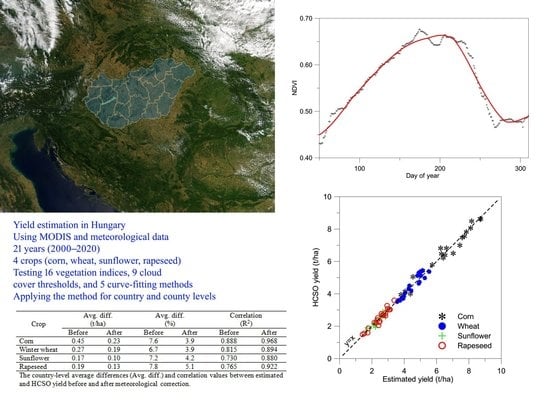
Testing the Robust Yield Estimation Method for Winter Wheat, Corn, Rapeseed, and Sunflower with Different Vegetation Indices and Meteorological Data

Abstract

Remote sensing-based crop yield estimation methods rely on vegetation indices, which depend on the availability of the number of observations during the year, influencing the value of the derived crop yield. In the present study, a robust yield estimation method was improved for estimating the yield of corn, winter wheat, sunflower, and rapeseed in Hungary for the period 2000–2020 using 16 vegetation indices. Then, meteorological data were used to reduce the differences between the estimated and census yield data. In the case of corn, the best result was obtained using the Green Atmospherically Resistant Vegetation Index, where the correlation between estimated and census data was R² = 0.888 before and R² = 0.968 after the meteorological correction. In the case of winter wheat, the Difference Vegetation Index produced the best result with R² = 0.815 and 0.894 before and after the meteorological correction. For sunflower, these correlation values were 0.730 and 0.880, and for rapeseed, 0.765 and 0.922, respectively. Using the meteorological correction, the average percentage differences between estimated and census data decreased from 7.7% to 3.9%, from 6.7% to 3.9%, from 7.2% to 4.2%, and from 7.8% to 5.1% in the case of corn, winter wheat, sunflower, and rapeseed, respectively.

1. Introduction

The general and economic governance of modern societies requires that the state of key areas be monitored continuously, objectively, and as accurately as possible. One of the most important areas to be examined is the combination of natural and social resources within countries. Food production is highly important, and estimating the yield for the main crops is an essential element. Timely and reliable agricultural production forecasts are critical for food policy decisions and to enable rapid responses to emerging food shortfalls [1]. Almost all countries with significant agriculture established a crop estimation system, which was based essentially on the sum of terrestrial table-level observations and the reporting of producers. Since the 1970s, with the rapid spread of Earth observation satellites, it has been possible to examine the state of vegetation with satellite data, which have been proven to be a useful tool for agricultural applications. Remote sensing indicators are now widely used in agriculture for monitoring crop conditions and forecasting yield [2].

The methodology of the yield estimation procedures has a wide range [3]. Crop estimation models using satellite data can basically be divided into two groups, direct and indirect methods [4]. The indirect methods incorporate the satellite data into existing agrometeorological or crop growth models [5,6,7,8,9,10]. Many of these models require a significant amount of input data which limits their usefulness for research [11]. The direct models provide explicit mathematical relations between the satellite data and the yield of the given plant, where some of them also include some basic meteorological or agronomical data in the relationship [12,13,14,15,16]. The procedures are applied for various species, for example, for corn [17,18,19,20], wheat [21,22,23,24,25], barley [26,27], rice [28,29], millet [30,31], soybean [32,33,34], sorghum [35], sugar beet [36], canola [37,38,39], cotton [40], potato [41,42], sunflower [43,44], peanut [45], grape [46], or even for opium [47].

Low-resolution remote sensing data have been widely used in crop yield forecasting and monitoring [48]. High temporal frequency combined with broad spatial coverage and low cost has made these datasets a preferred choice for national and regional scale applications [11]. In order to establish sufficiently accurate crop estimation models, it is also important that satellite data are available over a longer time period. Therefore, in the past, studies have been based generally on NOAA AVHRR (National Oceanic and Atmospheric Administration Advanced Very High-Resolution Radiometer) data, while in recent years, primarily on MODIS (Moderate Resolution Imaging Spectroradiometer) data. Currently, many research activities on yield estimation are based on data from the Sentinel-2 satellites [49], but at present, there is still no available long time series in contrast to the previous two sensors.

The most commonly used vegetation index (VI) in the literature is undoubtedly the Normalized Difference Vegetation Index [4], but there are many studies that compare other VIs as well [49,50,51,52,53,54,55]. The aim of the present study is (1) to test the robust crop estimation method developed by [36] for 4 crops (winter wheat, corn, sunflower, rapeseed) in Hungary using various VIs derived from 21-year-long MODIS data series in different observational circumstances, and (2) to examine how much the accuracy of the robust crop estimation method improves by supplementing satellite data with meteorological data. Our hypothesis was that in this way, the differences between the estimated and the official census yield data could be significantly reduced.

The effect of different meteorological parameters (temperature, precipitation, soil moisture, etc.) on crop growth is widely documented [56,57], but the joint application of meteorological data and remote sensing-based vegetation indices is a relatively new approach [16]. The statistical models generally perform more accurately by adding meteorological variables than the models using vegetation indices only [16,58,59,60]. In those studies, a mathematical combination of remotely sensed VIs and meteorological data was applied. In the present research, a different approach was used. It is well known that vegetation indices are closely related to meteorological data, as the state of vegetation is determined, among other factors, by meteorological conditions, which are reflected in the vegetation indices. Therefore, first, a robust crop estimation procedure was applied using satellite data only, looking for the vegetation index with the best results. Then, the correlation between the resulting crop yield errors, i.e., the difference between the estimated yield data and the census data provided by HCSO (Hungarian Central Statistical Office), and the meteorological data series were calculated to reveal how the accuracy of the yield estimation could be increased.

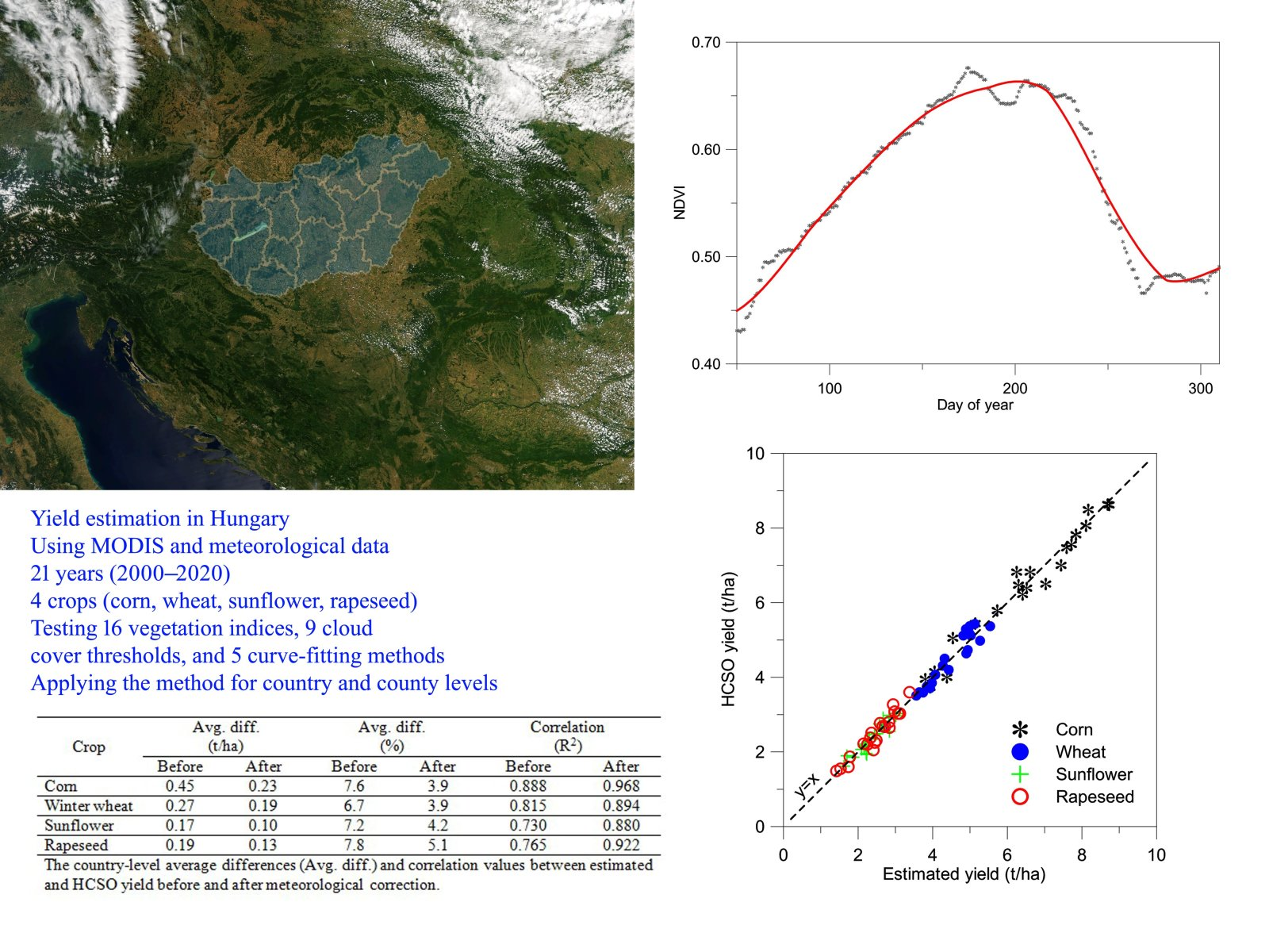
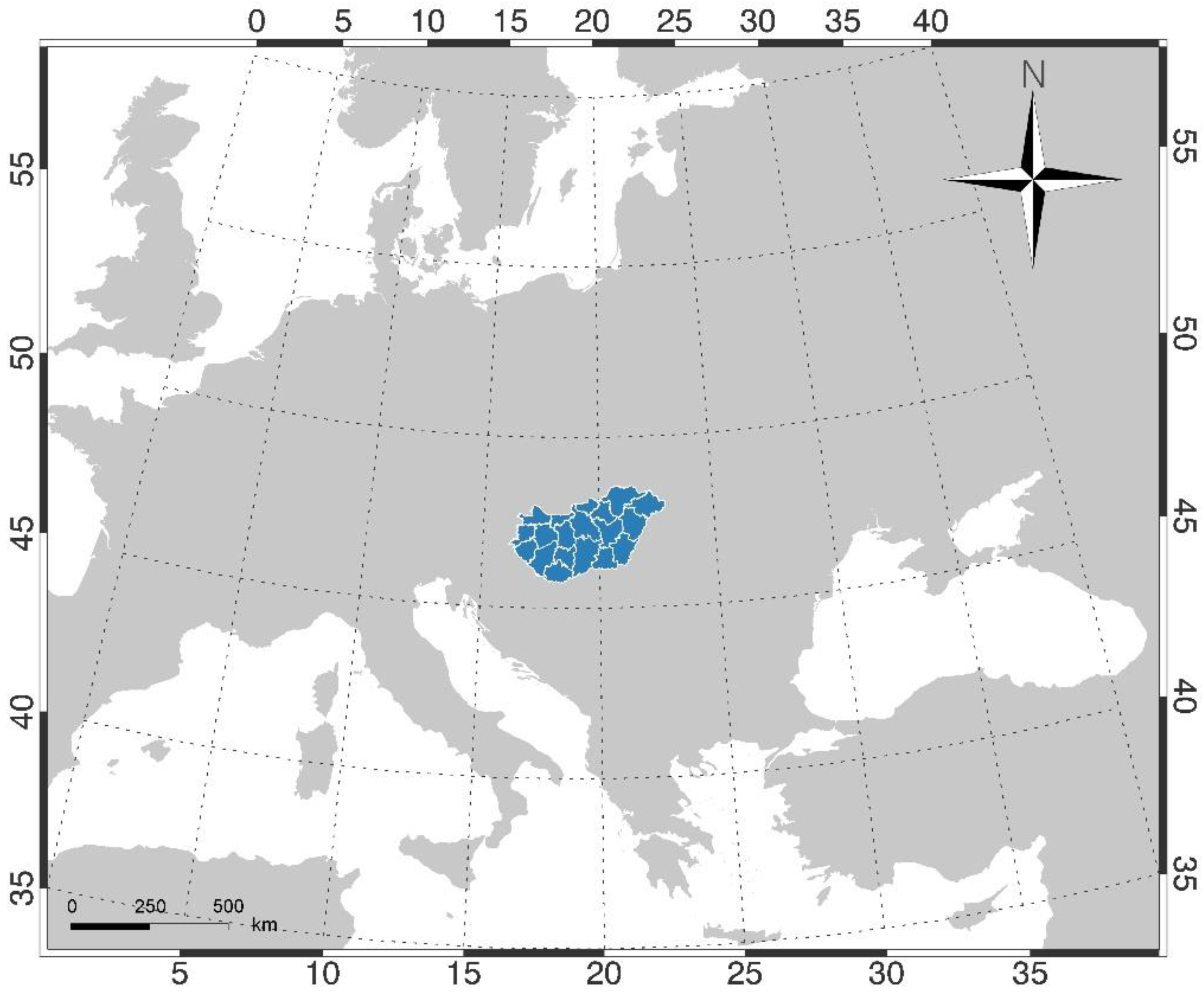
2. Study Area and Database Used

2.1. Study Area and Crop Information

The study area was the agricultural area of Hungary. Hungary is located in Central Europe (Figure 1), consisting of 19 counties (corresponding to the NUTS-3 level). The study was carried out on two levels: first for the whole country and then for the 19 counties. About 54% of Hungary’s land is agricultural land, 82% of which is used as arable land and 15% as grassland (https://www.ksh.hu/stadat_files/mez/en/mez0008.html (accessed on 5 May 2022)). The role of cereals and oilseeds in the crop structure is decisive. Our study covered the 4 crops with the largest acreage in Hungary in 2020: corn (ca. 981,000 ha), winter wheat (ca. 937,000 ha), sunflower (ca. 613,000 ha), and rapeseed (ca. 310,000 ha). The yield data needed to validate the yield estimation method were derived from the official HCSO reports (https://www.ksh.hu/stadat_files/mez/en/mez0018.html (accessed on 5 May 2022)).

2.2. Remote Sensing and Land Cover Database

The C006 MCD43A4 daily dataset derived from MODIS measurements was used in the present study to calculate area mean reflectances in MODIS Bands 1–7 for the period 2000–2020. The datasets were downloaded from LP DAAC [61]. The MCD43 Nadir Bidirectional Reflectance Distribution Function (BRDF)-Adjusted Reflectance (NBAR) is a daily dataset with 500 m spatial resolution, free from the view angle effects, resulting in a stable and consistent daily NBAR product. Country and county averaged mean reflectances of the agricultural areas were derived from cloud-free measurements.

To distinguish between agricultural and other land cover types at a yearly level, the MCD12Q1 MODIS Land Cover dataset of 2001–2019 was used on the same grid. For the years 2000 and 2020, the land cover information of the next and previous years was used, respectively. In addition, we used the CORINE 2012 (https://land.copernicus.eu/pan-european/corine-land-cover/clc-2012 (accessed on 24 February 2016)) dataset as well to take into account only those pixels which had at least a 90% share of “arable lands” categories.

To increase the accuracy of the yield forecasting, it would be ideal to have a vegetation index time series consisting of data that fully represent all agricultural areas in the investigated area (country or county) during the vegetation period. This kind of data can be obtained only for days when negligible cloud cover is present during the satellite overpass. Such days are few; therefore, the resulting vegetation index dataset might be insufficient for some periods. In addition, a higher cloud cover means that the average vegetation index value of the clear areas does not accurately represent the average vegetation index of the whole country (or county). In our previous studies [23,36], the threshold of 50% cloud cover value was applied, while in the present study, several cloud cover criteria (from 10% up to 90%) were also tested. The average annual data number as a function of cloud coverage is shown in Figure 2.

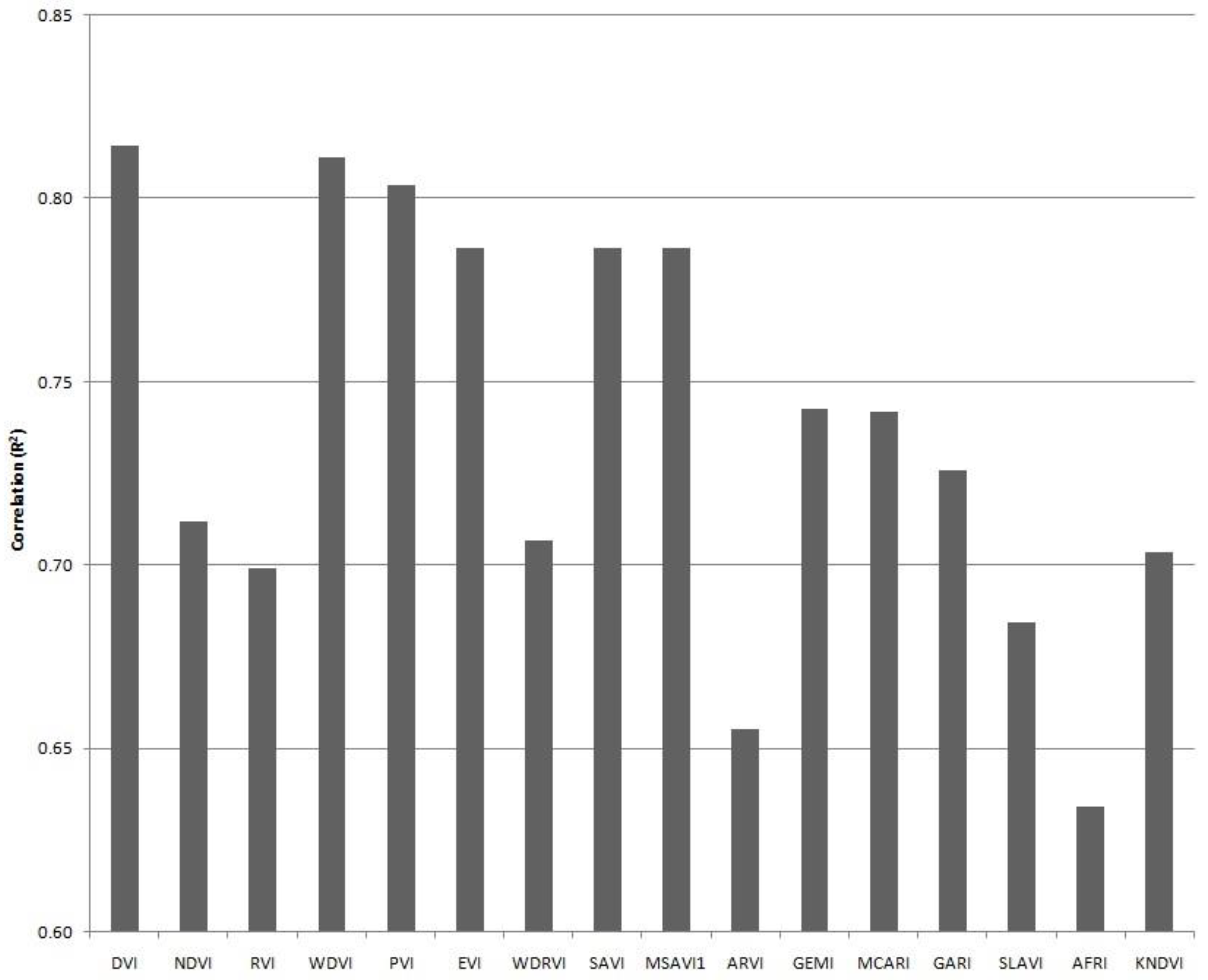
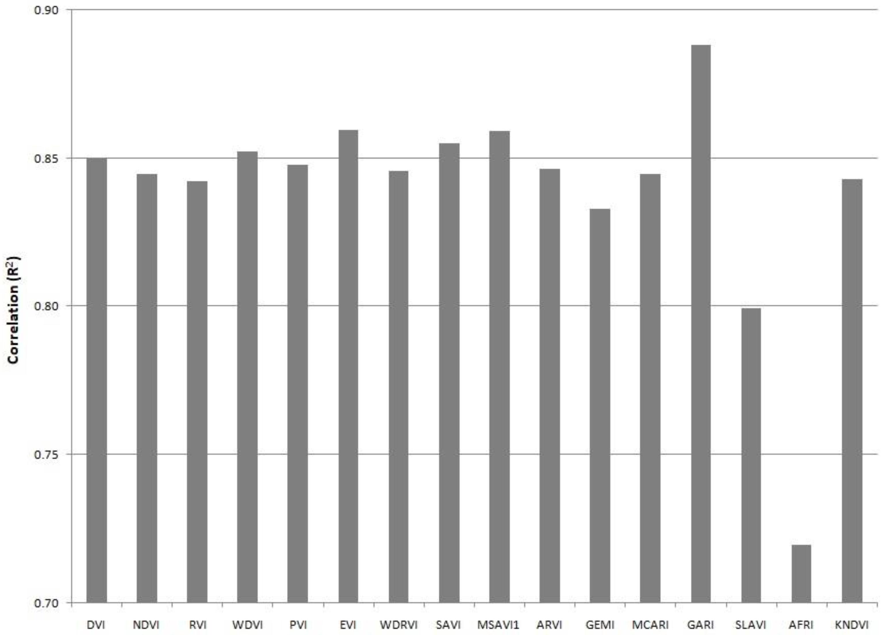
2.3. Vegetation Indices

Vegetation indices have been used since the beginning in the study of Earth’s surface and vegetation. VIs are mathematical transformations, usually ratios or linear combinations of reflectance measurements in different spectral bands, especially in the visible and near-infrared parts of the spectra [52]. Since the first VI (Ratio Vegetation Index, introduced by [62] in 1969, innumerable vegetation indices have been developed. From those, we selected 16 VIs to test the robust crop estimation method. In the formula of these indices, R_B, R_G, R_R, R_NIR (0.8–1.1 µm), and R_MIR2 (2–2.4 µm) are the reflectance values of MODIS band 3 (“blue”), 4 (“green”), 1 (“red”), 2 (“near-infrared”), and 7 (“middle-infrared”), respectively.

The vegetation indices used in the study are as follows:

(a) DVI—Difference Vegetation [63]

$$\mathrm{DVI}=R_{\mathrm{NIR}}-R_{\mathrm{R}}$$

(1)

DVI is one of the simplest VI, which is very sensitive to changes in soil background, and it can be applied to monitor the ecological vegetation environment [54]. The DVI was used to develop our robust yield forecasting method [36].

(b) NDVI—Normalized Difference Vegetation Index [64]

$$\mathrm{NDVI}=\frac{R_{\mathrm{NIR}}-R_{\mathrm{R}}}{R_{\mathrm{NIR}}+R_{\mathrm{R}}}$$

(2)

NDVI is the most common index for studying the condition of the surface and vegetation, which is a useful indicator of canopy structure, chlorophyll content, nitrogen content, fractional intercepted or absorbed PAR (Photosynthetically Active Radiation), and potential photosynthetic activity across a wide range of vegetation types [65].

(c) RVI—Ratio Vegetation Index [62]

$$\mathrm{RVI}=\frac{R_{\mathrm{NIR}}}{R_{\mathrm{R}}}$$

(3)

RVI is the earliest VI, which is widely used for green biomass estimations and monitoring, specifically at high-density vegetation coverage, since this index is very sensitive to vegetation and has a strong correlation with plant biomass [54].

(d) WDVI—Weighted Difference Vegetation Index [66]

$$\mathrm{WDVI}=R_{\mathrm{NIR}}-a\ast R_{\mathrm{R}},$$

(4)

where a is the slope of the soil line. WDVI can be used for estimating the leaf area index (LAI) of green vegetation. This WDVI offers a good correction for soil background in estimating the LAI of green vegetation, e.g., cereals at the vegetative stage [67]. The parameters of the soil line can be obtained by quantile regression [68,69].

(e) PVI—Perpendicular Vegetation Index (Richardson and Wiegand [63]

$$\mathrm{PVI}=\frac{R_{\mathrm{NIR}}-a\ast R_{\mathrm{R}}-b}{\sqrt{1+a^2}},$$

(5)

where a and b are the slope and intercept of the soil line, respectively. PVI filters out the effects of soil background in an efficient way and also has less sensitivity to atmospheric effects. It is mainly used for the inversion of surface vegetation parameters (grass yield, chlorophyll content), the calculation of LAI, and vegetation identification and classification [54].

(f) EVI—Enhanced Vegetation Index [70]

$$\mathrm{EVI}=\frac{2.5\ast \left(R_{\mathrm{NIR}}-R_{\mathrm{R}}\right)}{R_{\mathrm{NIR}}+6\ast R_{\mathrm{R}}-7.5\ast R_{\mathrm{B}}+1}$$

(6)

EVI was designed as an improvement of the NDVI under high green biomass conditions where NDVI saturates [71]. It used the blue reflectance band as well and was proposed to reduce both atmospheric and soil background noise simultaneously [72].

(g) WDRVI—Wide Dynamic Range Vegetation Index [73]

$$\mathrm{WDRVI}=\frac{c\ast R_{\mathrm{NIR}}-R_{\mathrm{R}}}{c\ast R_{\mathrm{NIR}}+R_{\mathrm{R}}}+1,$$

(7)

where c is the weighting coefficient, with a value ranging from 0.1 to 0.2. In this work, the average value, c = 0.15, was used. WDRVI was designed to improve the sensitivity of NDVI under these conditions. It was demonstrated that the sensitivity of the WDRVI to moderate-to-high LAI (between 2 and 6) was at least 3 times greater than that of the NDVI [71].

(h) SAVI—Soil Adjusted Vegetation Index [74]

$$\mathrm{SAVI}=\frac{\left(1+L\right)\ast \left(R_{\mathrm{NIR}}-R_{\mathrm{R}}\right)}{R_{\mathrm{NIR}}+R_{\mathrm{R}}+L},$$

(8)

where L is a canopy background adjustment factor. The value of L is 0 when the vegetation density is very high and L = 1 when the vegetation is scarce and soil reflection is high. In this study, L = 0.5 was used. SAVI attempts to minimize the influence of soil luminance, and it is used generally in areas where vegetative cover is low [75].

(i) MSAVI—Modified Soil Adjusted Vegetation Index [76]

$$\mathrm{MSAVI}=\frac{\left(1+L_1\right)\ast \left(R_{\mathrm{NIR}}-R_{\mathrm{R}}\right)}{R_{\mathrm{NIR}}+R_{\mathrm{R}}+L_1},$$

(9)

$$\mathrm{where} L_1=1-2\ast a\ast \left(\mathrm{NDVI}\right)\ast \left(\mathrm{WDVI}\right)$$

(10)

As the canopy background adjustment factor (L) should vary inversely with the amount of vegetation, MSAVI was developed with a variable L factor. The MSAVI is shown to increase the dynamic range of the vegetation signal while further minimizing the soil background influences, resulting in greater vegetation sensitivity as defined by a “vegetation signal” to “soil noise” ratio [76].

(j) ARVI—Atmospherically Resistant Vegetation Index [77]

$$\mathrm{ARVI}=\frac{R_{\mathrm{NIR}}-\left(R_{\mathrm{R}}-y\ast \left(R_{\mathrm{B}}-R_{\mathrm{R}}\right)\right)}{R_{\mathrm{NIR}}+\left(R_{\mathrm{R}}-y\ast \left(R_{\mathrm{B}}-R_{\mathrm{R}}\right)\right)} ,$$

(11)

where y is the so-called self-correcting factor. If no atmospheric data is present a priori, the y = 1 is a good choice for better adjustments [77]. The ARVI is commonly used to eliminate the effects of atmospheric aerosols.

(k) GEMI—Global Environment Monitoring Index [78]

$$\mathrm{GEMI}=d\ast \left(1-0.25\ast d\right)-\frac{R_{\mathrm{R}}-0.125}{1-R_{\mathrm{R}}},$$

(12)

$$\mathrm{where} d=\frac{2\ast \left(R_{\mathrm{NIR}}{}^2-R_{\mathrm{R}}{}^2\right)+1.5\ast R_{\mathrm{NIR}}+0.5\ast R_{\mathrm{R}}}{R_{\mathrm{NIR}}+R_{\mathrm{R}}+0.5}$$

(13)

The GEMI vegetation index has been designed specifically to reduce the relative effects of the undesirable atmospheric perturbations while maintaining the information about the vegetation cover [78].

(l) MCARI—Modified Chlorophyll Absorption in Reflective Index [79]

$$\mathrm{MCARI}=\frac{1.5\ast \left(2.5\ast \left(R_{\mathrm{NIR}}-R_{\mathrm{R}}\right)-1.3\ast \left(R_{\mathrm{NIR}}-R_{\mathrm{G}}\right)\right)}{\sqrt{{\left(2\ast R_{\mathrm{NIR}}+1\right)}^2-\left(6\ast R_{\mathrm{NIR}}-5\ast R_{\mathrm{R}}\right)-0.5}}$$

(14)

MCARI gives a measure of the depth of chlorophyll absorption and is very sensitive to variations in chlorophyll concentrations as well as variations in Leaf Area Index (LAI). MCARI values are not affected by illumination conditions, the background reflectance from soil, and other non-photosynthetic observed materials [80].

(m) GARI—Green Atmospherically Resistant Vegetation Index [81]

$$\mathrm{GARI}=\frac{R_{\mathrm{NIR}}-\left(R_{\mathrm{G}}-y\ast \left(R_{\mathrm{B}}-R_{\mathrm{R}}\right)\right)}{R_{\mathrm{NIR}}+\left(R_{\mathrm{G}}-y\ast \left(R_{\mathrm{B}}-R_{\mathrm{R}}\right)\right)},$$

(15)

where y is a parameter that controls the atmospheric correction. In this work, similarly as in the case of ARVI, y = 1 was used. GARI is tailored to the concept of ARVI and is expected to be as resistant to atmospheric effects as ARVI but more sensitive to a wide range of chlorophyll concentrations [81].

(n) SLAVI—Specific Leaf Area Vegetation Index [82]

$$\mathrm{SLAVI}=\frac{R_{\mathrm{NIR}}}{R_{\mathrm{R}}+R_{\mathrm{MIR}2}}$$

(16)

The middle-infrared band was included to supplement the relationship between red and NIR that forms the underlying principle of most vegetation indices [82]. Compared with NDVI, SLAVI is less affected by cloud shadows, which may remain even after cloud and cloud shadow masking [83].

(o) AFRI—Aerosol-free Vegetation Index [84]

$$\mathrm{AFRI}=\frac{R_{\mathrm{NIR}}-0.5\ast R_{\mathrm{MIR}2}}{R_{\mathrm{NIR}}+0.5\ast R_{\mathrm{MIR}2}}$$

(17)

AFRI’s main advantage is in penetrating an opaque atmosphere influenced by smoke due to biomass burning without the need for explicit correction for the aerosol effect [85].

(p) KNDVI—Kernel NDVI [85]

$$\mathrm{KNDVI}=\tanh \left({\left(\mathrm{NDVI}\right)}^2\right)$$

(18)

This brand-new index seems better qualified to cope with noise, saturation, and complex phenology than NDVI [86].

The time series of the 16 vegetation indices in 2020 can be seen in Figure S1, corresponding to the country’s means. Figure S2 shows the cross-plot of individual indices and NDVI, taking into account the entire period of time (2000–2020).

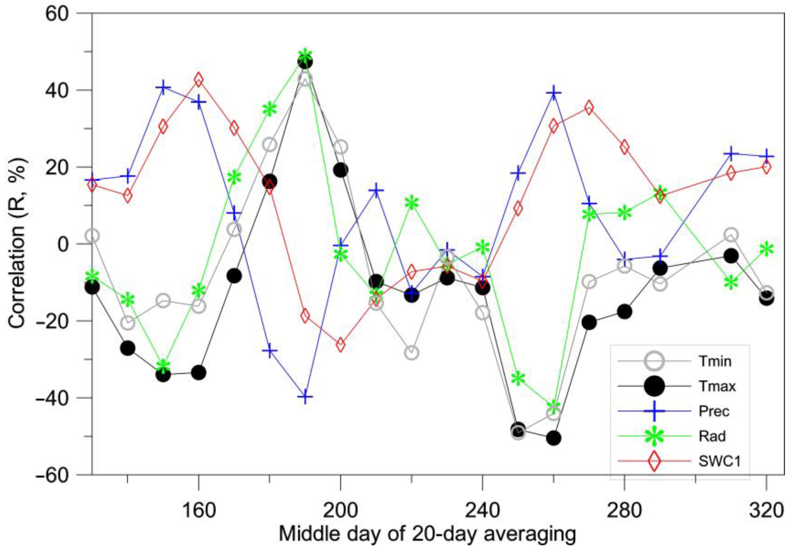
2.4. Meteorological and Soil Water Content Data

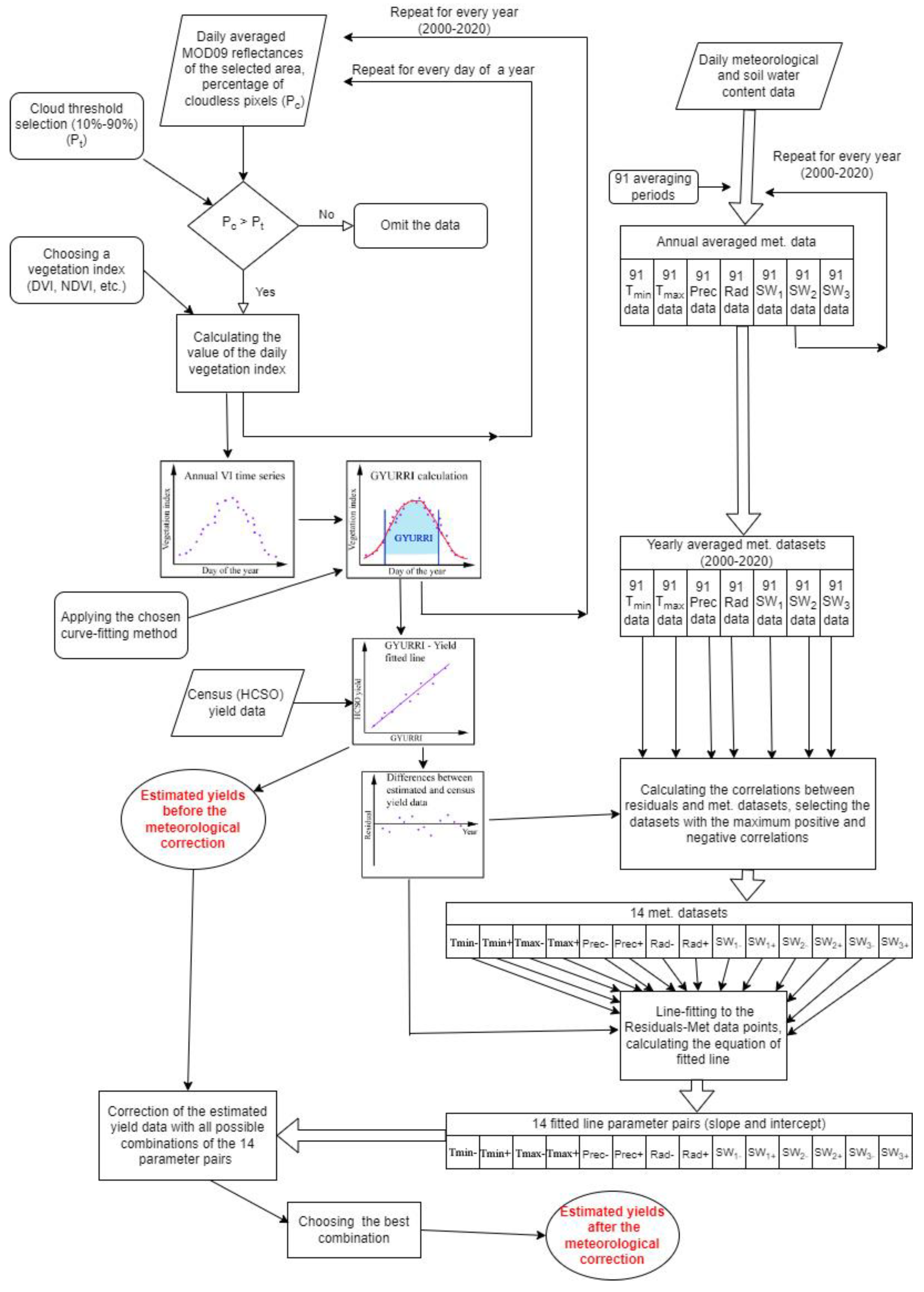
Hungary has a moderate climate with a mean annual temperature of about 10 °C and a mean annual precipitation of 500–700 mm. Daily meteorological data for 2000–2020 were obtained from the FORESEE v3.2 dataset [87], which contains daily minimum and maximum temperatures (T_min and T_max, respectively, [°C]) and precipitation sums (Prec [mm]) for the Carpathian basin with 1/6° × 1/6° spatial resolution. Daylight mean global radiation (Rad [W m⁻²]) was also calculated on the FORESEE grid using the MTClim model [88]. The 3 hourly ERA5-Land soil water content (SWC) data [m³ m⁻³] with 0.1° × 0.1° spatial resolution was downloaded for 3 soil layers (SWC₁ from 0–0.07 m, SWC₂ from 0.07–0.28 m, and SWC₃ from 0.28–1 m depth) from the Copernicus site (https://cds.climate.copernicus.eu/cdsapp#!/dataset/reanalysis-era5-land?tab=overview (accessed on 16 March 2021)) for 2000–2020. From the daily data stored at the original grid, country and county mean values were calculated.

Several averaged datasets were generated from the meteorological data, where the difference between the starting (D_b) and the final day (D_e) of the averaging varied from 20 days to 200 days. Thus, a total of 7 × 91 M(x, D_b, D_e) datasets were produced (Table S1), where M represents the averaged meteorological data between D_b and D_e and x is one of the above 7 parameters (T_min, T_max, Prec, Rad, SWC₁, SWC₂, SWC₃). Each of these M datasets consisted of 21 data, corresponding to the averaged values of the 21 years studied. For example, M (Prec, 120, 150) contains an annual time series of precipitation values averaged between DOYs (Day Of Year) 120 and 150.

3. Methodology

This study is based on the robust crop estimation method developed earlier, providing yield estimation of a larger area (such as a country or county). This procedure was first developed for NOAA AVHRR recordings using the DVI vegetation index [36] and later applied to MODIS NDVI data [23,25]. The fundamental point of this method is that there is no need for a detailed classification to identify the acreage of different crops since the general conditions of the vegetation-covered surfaces also represent the individual crop conditions in the case of the species with similar vegetation cycles [19,36,89].

In our current study, the method was applied to 4 plants (winter wheat, corn, sunflower, and rapeseed). In each case, the method was applied first to the whole country, then to the 19 counties. The first step is to fit a mathematically simple function on the spatially averaged VI values V(doy) between a beginning and ending day (d_b, d_e) to eliminate the stochastic fluctuation of the individual vegetation index data (Bognár et al., 2017). The value of d_b and d_e depends on the vegetation cycle of the given plants. In this work, 5 different curve fitting procedures were applied:

(a) Double Gauss curves

The function to describe the V(doy) function with two Gaussian curves looks like:

$$V_{\mathrm{Gauss}}\left(d\right)=V_{\mathrm{FixedSoil}}+G_1\left(d\right)+G_2\left(d\right),$$

(19)

$$\mathrm{where} G_i\left(d\right)=A_i·e^{{\frac{-\left(d-d_i\right)}{{\sigma }_i^2}}^2},$$

(20)

and V_FixedSoil is a pre-selected constant. To get the best least square deviation curve, there are six parameters to be fitted here (A_i, d_i, σ_i).

(b) Lagrange interpolation

Since the raw data often contains errors, like unexplainable jumps on the index curves, the data is smoothed with an averaging method. For exact interpolation methods, using only the raw data often resulted in obviously false curves, so we decided they must be applied on averaged or smoothed curves, which we call here the “averaged dataset”. This averaged dataset is created with an interval length parameter typically around 10 days. A simple algorithm coalesces adjacent data points within this length into subsets of data, making the averages of this subset constitute the points in the “averaged dataset”.

Then, on this “averaged dataset”, a simple low degree (usually 2–4) Lagrange interpolation gives the resulting approximation function V_Lagrange(d).

(c) Cubic spline function

The cubic spline function is built on the same “averaged dataset” as the Lagrange function. The approximation V_CubicSpline(d) function is got by cubic spline calculation on these averaged points.

(d) Smoothed function

Its main parameter is a “smoothing width” (D_s) given in days. Smoothing is achieved by a Gaussian weight function. The function approximation is the following:

$$V_{\mathrm{Smoothed}}\left(d\right)=\frac{1}{W}{\displaystyle \sum }_{d_b}^{d_e}w\left(-d\right)·\left(d\right),$$

(21)

$$\mathrm{where} w\left(-d\right)=e^{-{\left(\frac{-d}{D_s}\right)}^2}, \mathrm{and}$$

(22)

$$W={\displaystyle \sum }_{d_b}^{d_e}w\left(-d\right)$$

(23)

The summation from d_b to d_e goes through only on the existing days in the data.

(e) Raw function

Raw function is basically a step function, having constant values (V(d_i)) around the existing points in the [(d_i−1 + d_i)/2, (d_i + d_i+1)/2)] intervals.

The different fitted curves to the NDVI time series in 2020 can be seen in Figure 3.

As a next step, the matched vegetation index values were integrated between a properly chosen starting and end day. The general form of the General Yield Unification Robust Reference Index (GYURRI) (Ferencz et al., 2004 [36]) obtained in this way is:

$$GYURRI={{\displaystyle \int }}_{d_1}^{d_2}{V}_k\left(t\right)dt,$$

(24)

where t is measured in day units, V_k(t) is the value of fitted curve, d₁ and d₂ are the first and last days of the integral, and k is the applied fitting method (Gauss, Lagrange, etc.). The procedure was applied to the 16 vegetation indices for the series obtained with the separate cloud coverage criterion, in each case using the 5 fitting methods, testing their different input parameters. Then, the Pearson’s R correlation value between the resulting GYURRI values and HCSO yield data were calculated, assuming a linear relationship between the two series. Thus, we obtained which vegetation index and which curve matching had the highest correlation value. Using this vegetation index-curve fitting, the differences between estimated and actual (HCSO) yield data were calculated and defined as R datasets:

$$R_i=Y_i-K_i ,$$

(25)

where Y_i and K_i are the estimated and HCSO yield data in the year i (i = 2000–2020). In the next step, the resulting R series was correlated with the 7 × 91 meteorological data series (M) mentioned in point 2.4, again assuming a simple linear relationship. For all 7 meteorological parameters, the largest number of positive and negative correlations out of 91 cases were selected (7 × 2 = 14 datasets). In these meteorological data–residual data points, the parameters of the fitted line were calculated by linear fitting. With all possible combinations of these, the estimated yields were corrected, looking for the smallest deviations from the actual yield. The corrected yield data was calculated as follows:

$$Y_{\mathrm{new}}=Y_{\mathrm{old}}-{\displaystyle \sum }_{i=1}^h(a_i\ast M_i+b_i),$$

(26)

where Y_new and Y_old are the estimated yield data after and before the correction, M_i is the corresponding meteorological data, a_i and b_i are the above-mentioned slope and intercept of the fitted line, and h is the number of corrections. The correction was calculated first for h = 1 (14 cases), then h = 2 (14 × 13 cases), then h = 3 (14 × 13 × 12 cases), and so on until h = 14. With the corrected yield data obtained, the average deviations over the 21 years between the estimated and HCSO yield data were calculated, searching for the lowest average difference between Y_new and HCSO yield data. The flowchart of the applied methodology can be seen in Figure 4.

4. Results

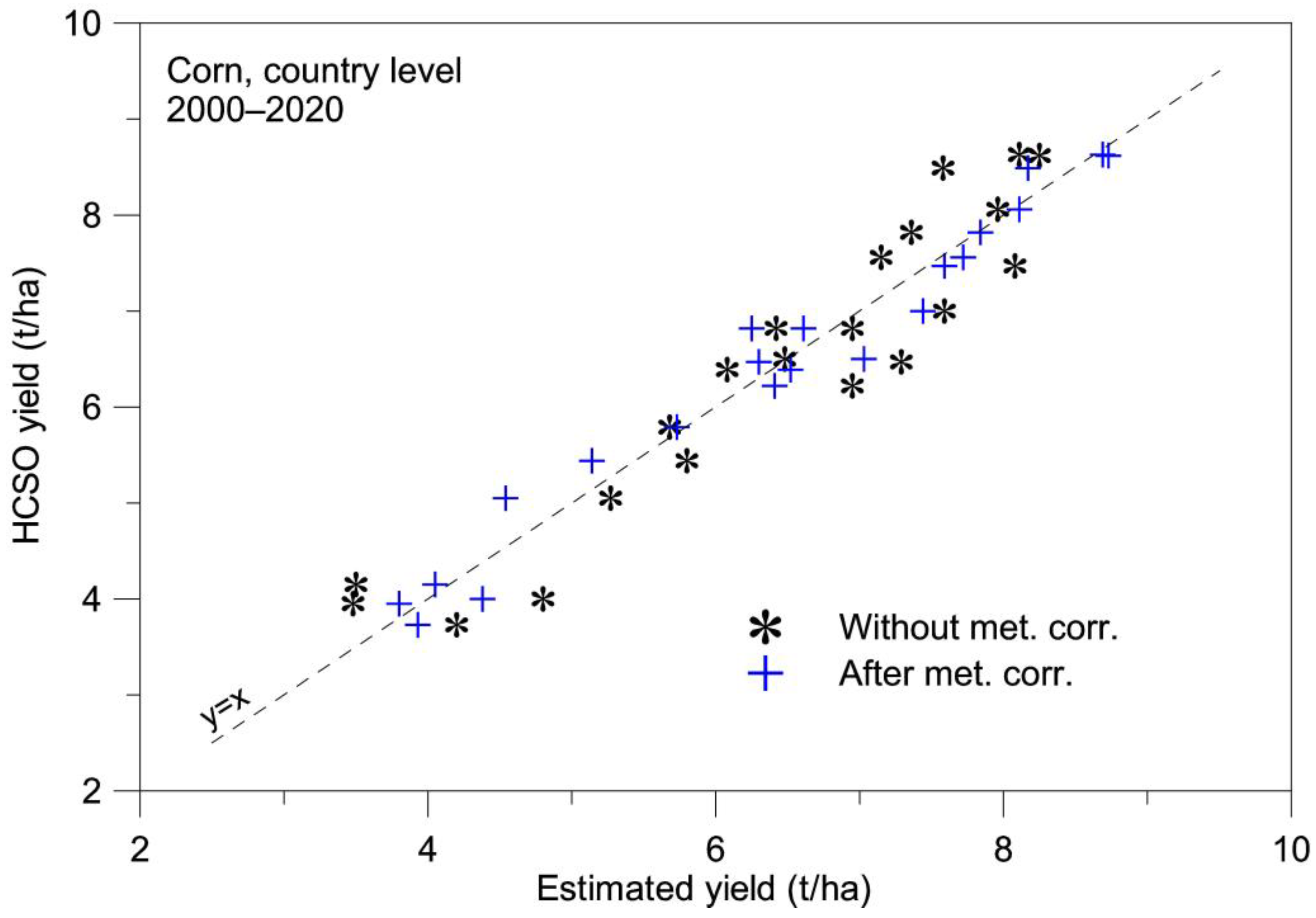
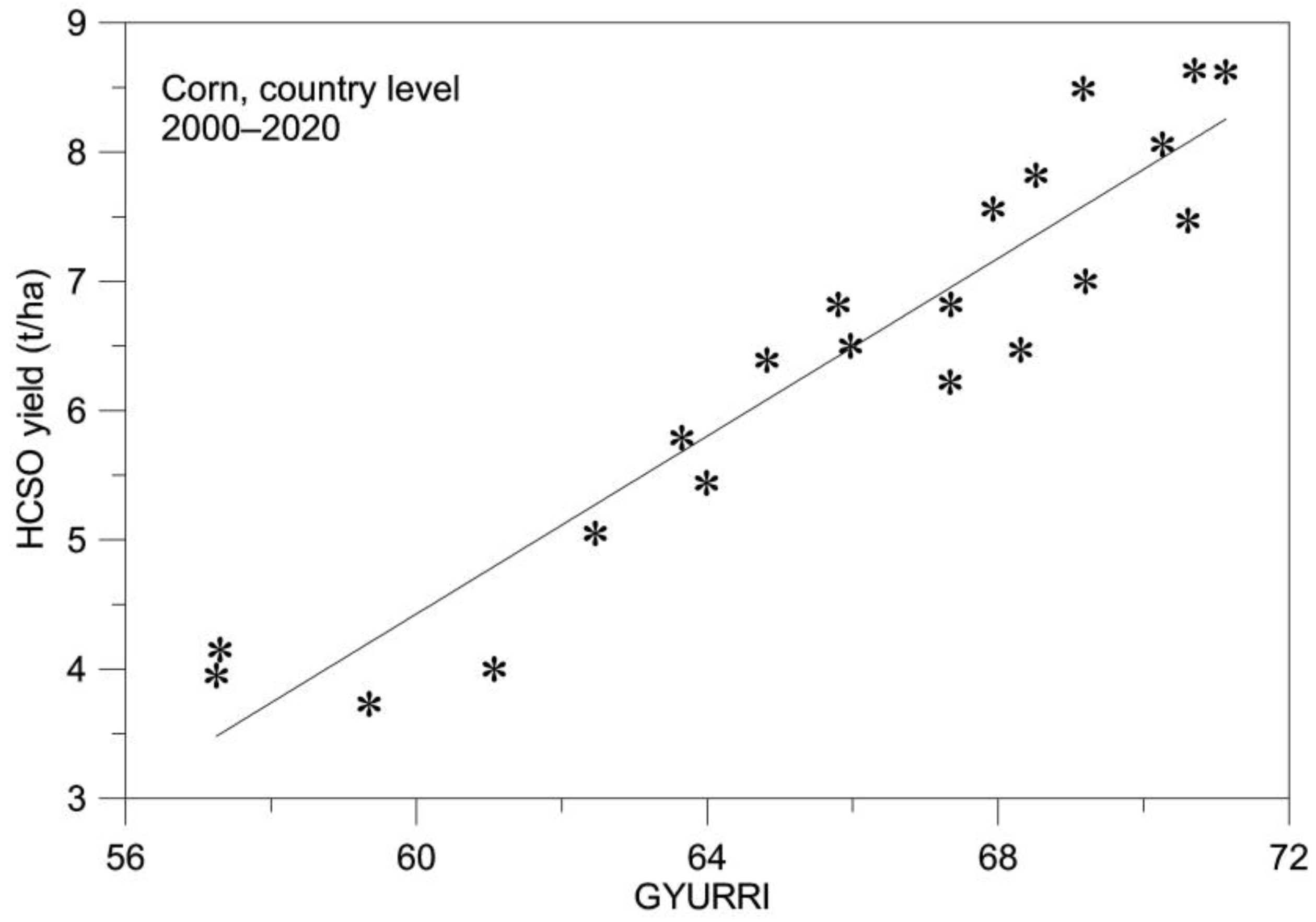
4.1. Corn, Country Level

Corn has the largest acreage in Hungary. In the last 21 years, the national average yield of corn in Hungary has ranged from 3.73 t/ha (2007) to 8.63 t/ha (2016). The sowing of corn usually begins in April, and the harvesting time varies between mid-September to mid-November. This would suggest that the end date of curve fitting should be around d_e = 315, but we would like to provide an accurate yield forecasting as early as possible; therefore, the starting and ending of curve fitting were selected as d_b = 100 and d_e = 270.

The robust yield estimation method was applied for all possible combinations of the 4 crops, 16 vegetation indices, 9 cloud coverage criteria, and 5 curve fitting methods, looking for the highest correlation value between the calculated GYURRI and HCSO yield data. Applying the 16 VIs, it was found that the correlation values were roughly the same for 13 VIs; the R² values were between 0.830 and 0.860. In the case of two indices that use the middle-infrared band (SLAVI, AFRI), the correlation values were much lower (Figure 5). However, with GARI, a remarkably high correlation value (R² = 0.888) was obtained; therefore, in the case of corn, the use of GARI was proven to be the most effective. Examining the cloud coverage thresholds, it was found that the best result was obtained at the 30% cloud cover threshold, that is, when we include only the days when the cloud cover was less than or equal to 30% over the country (Figure S3).

Applying different curve fitting methods, the best result was obtained when the Lagrange curve fitting was applied using a third-degree curve with a 50-day averaging (Table S2). In this case, the start and final days of integration were d₁ = 102 and d₂ = 244. The best result for corn was obtained using the 30% cloud cover criterion, GARI vegetation index, and third-degree Lagrange curve fitting. In this case, the correlation between the calculated 21 GYURRI values and the actual yield data provided by HCSO was R² = 0.888 (Figure 6). The average difference between estimated and actual yield was 0.45 t/ha, and the average percentage difference was 7.65%. In the following calculations, the year-by-year differences (‘residuals’) between the estimated and the HCSO data (R dataset) were used.

In the next step, the correlation values between the R datasets and the 91 M data series were calculated, selecting the M datasets with the highest positive and negative correlations for each meteorological parameter separately. This way, 7 × 2 = 14 M datasets were selected. These correlation values were low; the highest value (−50.43%, R² = 0.254) was obtained in the case of M(T_max, 250, 270) dataset (Table S3). As an example, Figure 7 shows correlations between the R dataset and the 20-day averages of different meteorological parameters.

Next, a line was fitted to the M-R data pairs in the case of each 14 M data series, calculating the slope and intercept of the fitted lines. For example, in the case of the M(T_max, 250, 270) dataset, the slope and intercept of the fitted line were a_Tmax,250,270 = 0.111, and b_Tmax,250,270 = 2.502, respectively (Figure S4). The R series was then corrected with all possible combinations of the 14 M series (Equation (26)). As our experience has shown that more than 4 corrections no longer improve results, the correction was calculated first for h = 1 (14 cases), then h = 2 (14 × 13 cases), then h = 3 (14 × 13 × 12 cases), and finally h = 4 (14 × 13 × 12 × 11 cases). With the corrected yield data obtained, the average deviations over the 21 years between the estimated and HCSO yield data were calculated. In the case of corn, more corrections (h > 2) gave no better results. For h = 2, the best result was obtained by using T_min− (i.e., M(T_min, 240, 260)) and T_max+ (i.e., M(T_max, 180, 200)) together; this way, the average difference between the estimated and the HCSO yield was 0.297 t/ha (Table S4). For corn, the best result was obtained by using 4 meteorological datasets, namely M(T_min, 240, 260), M(T_max, 180, 200), M(Rad, 250, 270), and M(SWC₁, 150, 170). Applying these, the average difference between the adjusted estimated yield data and the HCSO yield data decreased to 0.228 t/ha and the average percentage difference to 3.9%, while the correlation increased from R² = 0.888 to R² = 0.968 (Figure 8).

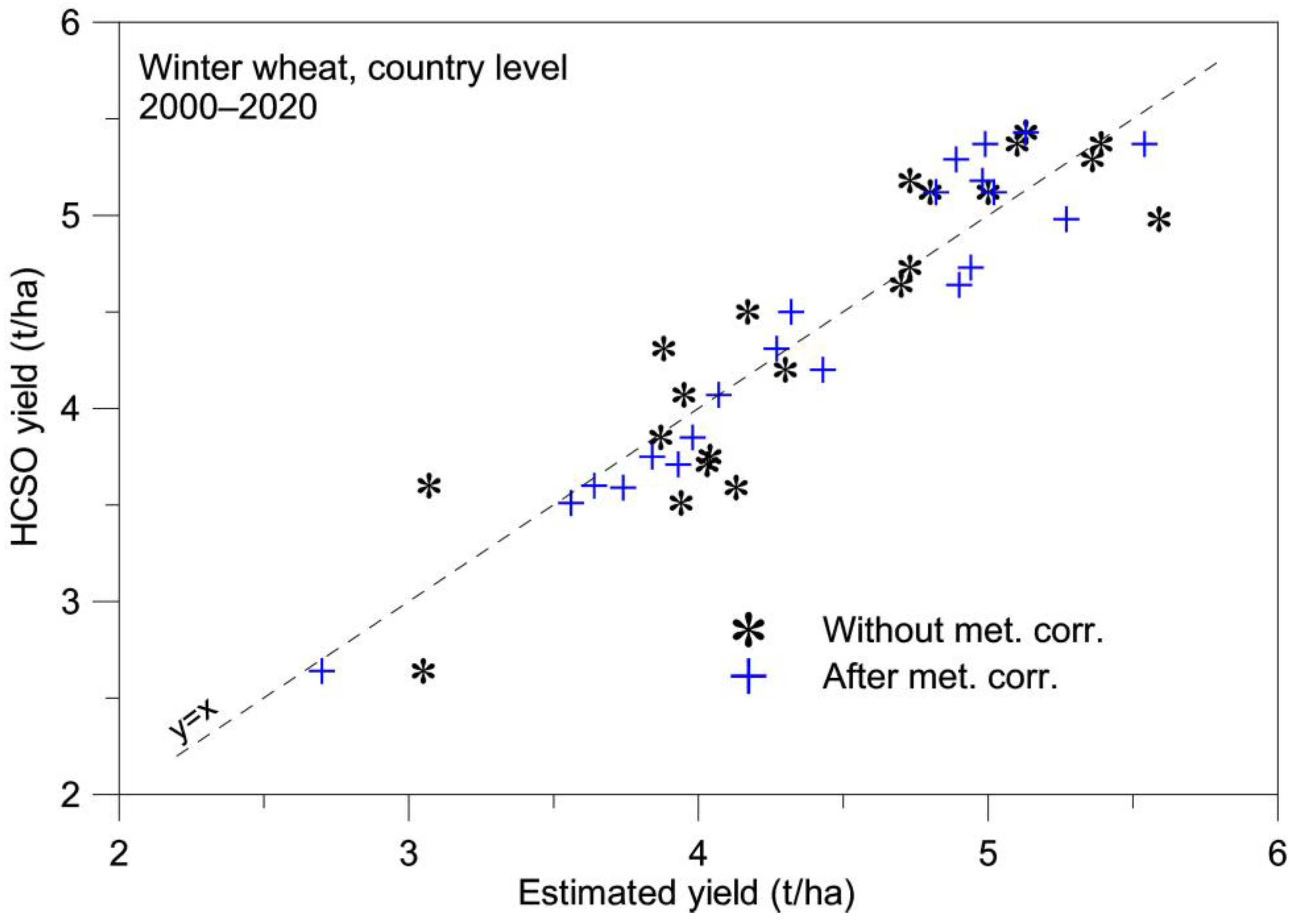
4.2. Winter Wheat, Country Level

Winter wheat has the second-largest sowing area in Hungary. In the last 21 years, the national average yield of winter wheat has ranged from 2.64 t/ha (2003) to 5.43 t/ha (2017). The harvesting of the winter wheat in Hungary begins around the end of June; therefore, the starting and final days of curve fitting have been selected as d_b = 45 and d_e = 185. Applying the 16 VIs (Figure 9), the two highest correlation value was obtained in the case of DVI (R² = 0.815) and WDVI index (R² = 0.811). The lowest value—similarly to the case of corn—was found using the AFRI index (R² = 0.634), and the correlation using the NDVI index proved to be exceptionally low (R² = 0.712).

Using the DVI datasets with different cloud cover criteria, the result was different from corn. It was found that the best correlation was obtained by applying the dataset with the highest cloud cover threshold (90%), which means that even data from days where 90% of the country was covered by cloud were used (Figure S5). One of the possible reasons for this may be that the curve fitting method is sensible for the data gaps in the rising part of the curve (Figure S6). It seems that in the case of winter wheat, for accurate yield estimation, it is more important to have a sufficient amount of measured data, knowing that the average vegetation index value of the clear areas presumably does not represent the average vegetation index of the whole country accurately.

Applying the 5 different curve fitting methods, the best result was obtained using the third-degree Lagrange curve fitting with a 60-day averaging (R² = 0.815). In the case of cubic spline, smoothed, and double-Gaussian curve fitting, the correlations were of almost equal value (R² =0.773, 0.771, and 0.766, respectively), while the lowest correlation was obtained using the raw fitting (R² = 0.745). Using the DVI dataset with a 90% cloud cover criterion and applying the third-degree Lagrange curve fitting method, the average difference between estimated and actual yield was 0.27 t/ha, and the average percentage difference was 6.67%.

In the following, the procedure was the same as it was in the case of corn. The highest correlation between the R and M datasets was R² = 0.435 using the M(T_min+, 140, 180) data series (Table S5). In the case of T_max negative, in the case of SWC₃ positive correlation values did not occur. The lowest average difference between corrected and HCSO yield data were obtained using 2 M series: M(T_min, 140, 180) and M(Rad, 140, 160). Applying these, the average difference between the adjusted estimated yield data and the HCSO yield data decreased to 0.19 t/ha and the average percentage difference to 3.92%, while the correlation increased from R² = 0.815 to R² = 0.894 (Figure 10).

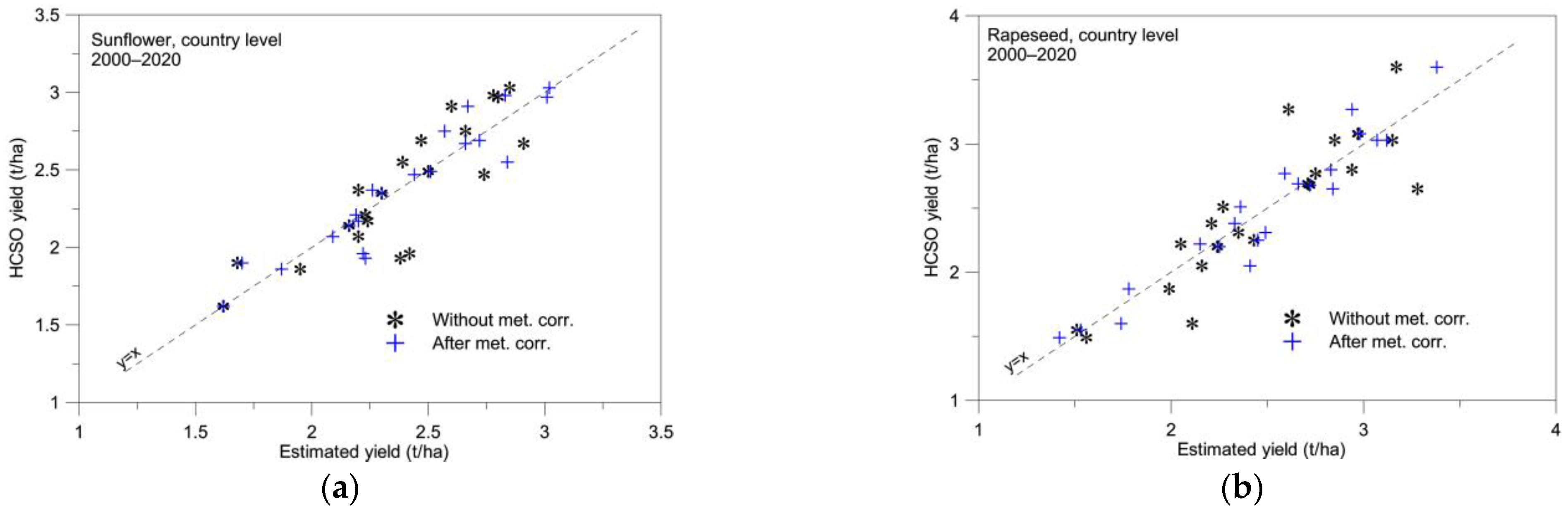
4.3. Sunflower and Rapeseed, Country Level

Sunflower has the third-largest sowing area in Hungary. In the last 21 years, the national average yield of sunflowers has ranged from 1.62 t/ha (2000) to 3.03 t/ha (2019). The vegetation cycle of sunflower is similar to the cycle of corn, but the harvesting begins a little bit earlier, at the beginning of September; therefore, the final day of curve fitting has been chosen as d_e = 240. The acreage of rapeseed has nearly tripled in the last 20 years; now, it has the fourth-largest sowing area in Hungary. The lowest yield of rapeseed between 2000 and 2020 was 1.49 t/ha in 2003, and the highest was 3.6 t/ha in 2016. The harvesting time of winter wheat and rapeseed is similar; therefore, the same d_b and d_e were used for the curve fitting. Varying the different VIs, similar results were obtained for sunflower as in the case of corn, and the best correlation was achieved using the GARI vegetation index. In the case of rapeseed, the DVI vegetation index produced the best result, as it was in the case of winter wheat. In both cases, the lowest correlation was obtained by applying AFRI (Figure S7).

Looking for the best correlation using datasets with different cloud coverage criteria, in the case of sunflower, the 20% cloud cover threshold produced a slightly better result than using the limit of 30% (as it was in the case of corn), while in the case of rapeseed the best result was obtained using the dataset with cloud cover criterion of 90%, as it was in the case of winter wheat. Finally, in both cases, the highest correlation was obtained by applying the third-degree Lagrange curve fitting method; the value of R² was 0.730 and 0.765 in the case of sunflower and rapeseed, respectively. Correction with meteorological data was also applied to these two plants. In the case of sunflower, the applied M datasets were M(T_min, 200, 260), M(Prec, 180, 200), and M(Rad, 150, 170). In the case of rapeseed M(T_max, 75, 125), M(Prec, 110, 130), and M(SWC₂, 60, 80) datasets were used. Applying these, the average difference between the adjusted estimated yield data and the HCSO yield data decreased from 0.168 t/ha to 0.097 t/ha, the average percentage difference from 7.19% to 4.19% in the case of sunflower. In the case of rapeseed, the average difference between the corrected estimated yield data and the HCSO yield data decreased from 0.192 t/ha to 0.125 t/ha, the average percentage difference from 7.82% to 5.14%. The correlation values increased to R² = 0.880 and R² = 0.922 (Figure 11).

4.4. Data Series of 19 Counties

The robust yield estimation method was applied for the data series of the 19 Hungarian counties. For each crop, the same variables were applied as for the dataset of Hungary. For the meteorological correction, the meteorological datasets of the given counties were applied. The analysis was based on 21-year data from 19 counties (21 × 19 = 399 data points for each crop). As expected from our previous investigations [19,36], the obtained average differences between the estimated and HCSO yield data were higher than in the case of the whole country (

Table 1. The county-level average differences (Avg. diff.) and correlation values between estimated and HCSO yield before and after meteorological correction.

Crop	Avg. Diff. (t/ha)		Avg. Diff. (%)		Correlation (R2)
	Before	After	Before	After	Before	After
Corn	0.60	0.48	11.1	9.0	0.825	0.883
Winter wheat	0.38	0.32	9.2	7.6	0.736	0.809
Sunflower	0.22	0.19	9.6	8.3	0.648	0.743
Rapeseed	0.35	0.31	16.7	14.4	0.570	0.672

), but in each case, better results were obtained using the meteorological correction (Figure 12). Except for rapeseed, in the case of the other three crops, the average differences between the estimated and HCSO yield data were lower than 10% after the meteorological correction.

5. Discussion

In the present study, the previously developed robust yield estimation method [19] was applied for the four crops with the largest sowing area in Hungary for the 2000–2020 period. In the procedure, 16 different MODIS-derived vegetation indices and 5 different curve fitting methods with 9 different cloud coverage criteria were tested. It was found that the simplest vegetation index, the DVI, provided the best results for autumn-sown crops (winter wheat and rapeseed), but the results were only slightly worse using the WDVI, PVI, EVI, SAVI, and MSAVI indices. The weakest correlation between the estimated and census (HCSO) yield data was obtained applying the ARVI, SLAVI, and AFRI indices, indicating that the use of the data of medium-infrared channels does not improve the accuracy of the yield estimation procedure. However, it is somewhat surprising that the correlation value for the NDVI vegetation index, the one most often used in yield estimation methods, was much lower than for the DVI index. The obtained correlation for winter wheat was R² = 0.815 and 0.712, while for rapeseed, R² = 0.765 and 0.627 using DVI and NDVI, respectively. In the case of spring-sown crops (corn and sunflower), the use of the GARI vegetation index obviously gave the best results. Among the 16 indices examined, GARI is the only one that uses near-infrared data together with all three visible channels (blue, green, and red). In these cases, too, the weakest correlation was obtained by applying the two indices that use the data of medium-infrared channels (SLAVI and AFRI). For both crops, DVI also gave better results than NDVI. Examining the cloud cover threshold, it was found that in the case of autumn-sown crops, it was important to have as much data as possible during the steeply rising section of the vegetation index curves in spring, so the use of the 90% cloud cover criterion seemed expedient here (Figure S5). For spring-sown crops, where this ascending part in vegetation index values is not present, datasets representing larger areas of the country gave better results. Thus, the best results were obtained using the 30% cloud criterion for corn (Figure S3) and 20% for sunflowers. In our previous study [23], the 50% cloud criterion gave the best results for winter wheat, but in this present work, the MODIS MCD43 dataset was used instead of MOD09, and the MCD43 dataset is much more efficiently purified from atmospheric and other effects. This could be the reason why this time, the Lagrange-type curve fitting produced the best results for all four crops instead of the previously used double-Gaussian curve fitting. Another aim of this study was to investigate the extent to which the accuracy of crop estimation can be improved by including meteorological (temperature, rainfall, radiation) and environmental (soil water content) data. For this, meteorological data were averaged between a starting and a final day in all 21 years studied. In the studies using statistical modeling with meteorological data for yield estimation, the averaging length of the parameters usually covers the growing season of the given crop [90,91,92] or monthly averages [46,93]. In this present study, more averaging lengths were tested; the length of averaging ranged from 20 to 200 days. Thus, by varying the start and end days, 91 time series were created for each variable (M datasets). For each crop, an R dataset was generated that contained the difference between the yield data estimated in the first step and the data provided by HCSO. Correlations between M and R datasets were then calculated, and for each meteorological parameter (including the soil moisture data), the datasets with the highest positive and negative correlations were selected. For these datasets, the parameters of the line fitted to the M-R data pairs were determined, and the estimated yield data were corrected using these parameters. The results have shown that the average difference between estimated and actual yield data could be significantly reduced by applying two, three, or four corrections together. These average differences were around 4% for 3 plants, while the difference was 5.1% for rapeseed (

Table 2. The country-level average differences and correlation values between estimated and HCSO yield before and after meteorological correction.

Crop	Avg. Diff. (t/ha)		Avg. Diff. (%)		Correlation (R2)
	Before	After	Before	After	Before	After
Corn	0.45	0.23	7.6	3.9	0.888	0.968
Winter wheat	0.27	0.19	6.7	3.9	0.815	0.894
Sunflower	0.17	0.10	7.2	4.2	0.730	0.880
Rapeseed	0.19	0.13	7.8	5.1	0.765	0.922

). For the 4 crops, the differences were reduced by an average of 3% (from 7.3% to 4.3%) using meteorological corrections. The correlation values were R² = 0.968, 0.894, 0.880, and 0.922 in the case of corn, winter wheat, sunflower, and rapeseed, respectively.

For comparison, Gornott and Wechsung [91], using their simple series model for Germany from 1992 to 2010, obtained a correlation value (R²) of 0.86 for winter wheat. Schauberger et al. [94] simulated winter wheat and corn yields in Hungary and got the R² = 0.86 for corn but only around 0.4 for winter wheat. Kern et al. [16] used meteorological data and soil water content in monthly resolution together with MODIS NDVI and annual fertilization amount data in Hungary for the 2000–2016 time period and obtained the R² values 0.901 for corn, 0.859 for winter wheat, 0.829 for sunflower, and 0.864 for rapeseed. Zhu et al. [95] combined agrometeorological indexes and remote sensing parameters to build a corn yield estimation model for two Chinese provinces; the obtained R² values were 082 and 0.74. Bojanowski et al. [96] used MODIS and Sentinel-3 data with agrometeorological indicators in Poland, and after leave-one-year-out cross-validation for the 2000–2019 period, the obtained R² values were 0.84 for winter wheat, 0.47 for rapeseed, and 0.51 for corn.

In addition to the national datasets, the method was also applied at the county (NUTS-3) level. The results confirmed our previous experience that the accuracy of the robust yield estimation procedure decreases when smaller area units are used. However, even for county datasets, the meteorological correction improved the accuracy of the estimates. The average percentage differences remained below 10%, except for rapeseed, where this difference was 14.4%. For the 4 crops as a whole, the average differences decreased to a lesser extent than the national one, by 1.82% (from 11.65% to 9.83%). It is important to note that in the case of Hungary, the estimation of county data has only scientific significance. Economically, the national yield estimation has outstanding importance. In summary, the robust yield estimation procedure, supplemented by meteorological correction, can be successfully applied to national yield estimation for the crops with the four largest sown areas. If the four crops are examined together (Figure 13), the correlation between the estimated and HCSO data is remarkably high, R² = 0.988.

6. Conclusions

This paper has presented a generalized approach to estimating crop yields with remote sensing and meteorological data. The results confirmed our initial hypothesis that the accuracy of the yield estimation could be improved by including meteorological data. It is important to note that the present study did not aim to explain the reasons behind the combination of the meteorological and environmental parameters which produced the best result. In the future, it will be worthwhile to carry out further studies to find out why the GARI index gave better results for spring-sown crops and why this did not occur for autumn-sown crops. It will also be worth exploring the possibility of combining vegetation indices with meteorological time profiles to produce a new dataset, which can be used as an input dataset in the robust yield forecasting method. This way, instead of the two-step method described in this paper—i.e., the results obtained using the VI data were corrected with the meteorological datasets—the yield forecasting procedure could be performed in one step.

The method presented in this study could be easily adapted for other countries and crop types as well; only the input parameters (e.g., the start and end days of curve-fitting) need to be adjusted to the given circumstances. In the future, it will be worthwhile to examine how the method can be applied to Sentinel-2 satellite data and how the accuracy of yield estimation is affected by less frequent time resolution but better spatial resolution.

References

1. Khamala, E. Review of the Available Remote Sensing Tools, Products, Methodologies and Data to Improve Crop Production Forecasts; FAO: Rome, Italy, 2017; ISBN 978-92-5-109840-0. [Google Scholar]
2. Khanal, S.; Kushal, K.C.; Fulton, J.P.; Shearer, S.; Ozkan, E. Remote sensing in agriculture—Accomplishments, limitations, and opportunities. Remote Sens. 2020, 12, 3783. [Google Scholar] [CrossRef]
3. Atzberger, C. Advances in Remote Sensing of Agriculture: Context Description, Existing Operational Monitoring Systems and Major Information Needs. Remote Sens. 2013, 5, 948–981. [Google Scholar] [CrossRef] [Green Version]
4. Basso, B.; Cammarano, D.; Carfagna, E. Review of Crop Yield Forecasting Methods and Early Warning Systems. In Proceedings of the First Meeting of the Scientific Advisory Committee of the Global Strategy to Improve Agricultural and Rural Statistics; FAO: Rome, Italy, 2013; pp. 15–31. [Google Scholar]
5. Wiegand, C.L.; Richardson, A.J.; Kanemasu, E.T. Leaf Area Index estimates for wheat from Landsat and their implications for evapotranspiration and crop modeling. Agron. J. 1979, 71, 336–342. [Google Scholar] [CrossRef]
6. Dorigo, W.A.; Zurita-Milla, R.; de Wit, A.J.W.; Brazile, J.; Singh, R.; Schaepman, M.E. A review on reflective remote sensing and data assimilation techniques for enhanced agroecosystem modeling. Int. J. Appl. Earth Obs. 2007, 9, 165–193. [Google Scholar] [CrossRef]
7. Reynolds, C.A.; Yitayew, M.; Slack, D.C.; Hatchinson, C.F.; Huete, A.; Petersen, M.S. Estimating crop yields and production by integrating the FAO crop specific water data and ground-based ancillary data. Int. J. Remote Sens. 2010, 21, 3487–3508. [Google Scholar] [CrossRef]
8. Curnel, Y.; de Wit, A.J.W.; Duvellier, G.; Defourny, P. Potential Performances of Remotely Sensed LAI Assimilation in WOFOST Model Based on an OSS Experiment. Agric. For. Meteorol. 2011, 151, 1843–1855. [Google Scholar] [CrossRef]
9. Nearing, G.S.; Crow, W.T.; Thorp, K.R.; Moran, M.S.; Reichle, R.H.; Gupta, H.V. Assimilating remote sensing observations of leaf area index and soil moisture for wheat yield estimates: An observing system simulation experiment. Water Resour. Res. 2012, 48. [Google Scholar] [CrossRef] [Green Version]
10. Huang, J.; Tian, L.; Liang, S.; Ma, H.; Becker-Reshef, I.; Huang, Y.; Su, W.; Zhang, X.; Zhu, D.; Wu, W. Improving winter wheat yield estimation by assimilation of the Leaf Area Index from Landsat TM and MODIS data into the WOFOST Model. Agric. For. Meteorol. 2015, 204, 106–121. [Google Scholar] [CrossRef] [Green Version]
11. Kasampalis, D.; Alexandridis, T.; Deva, C.; Challinor, A.; Moshou, D.; Zalidis, G. Contribution of remote sensing on crop models: A review. J. Imaging 2018, 4, 52. [Google Scholar] [CrossRef] [Green Version]
12. Maselli, F.; Conese, C.; Petkov, L.; Gilabert, M.A. Use of NOAA–AVHRR NDVI data for environmental monitoring of crop forecasting in the Sahel. Preliminary results. Int. J. Remote Sens. 1992, 13, 2743–2749. [Google Scholar] [CrossRef]
13. Hamar, D.; Ferencz, C.; Lichtenberger, J.; Tarcsai, G.; Ferencz-Árkos, I. Yield Estimation for Corn and Wheat in the Hungarian Great Plain Using Landsat MSS Data. Int. J. Remote Sens. 1996, 17, 1689–1699. [Google Scholar] [CrossRef]
14. Schut, A.G.T.; Stephens, D.J.; Stovold, R.G.H.; Adams, M.; Craig, R.L. Improved wheat yield and production forecasting with a moisture stress index, AVHRR and MODIS data. Crop. Pasture Sci. 2009, 60, 60–70. [Google Scholar] [CrossRef]
15. López-Lozano, R.; Duveiller, G.; Seguini, L.; Meroni, M.; García-Condado, S.; Hooker, J.; Leo, O.; Baruth, B. Towards regional grain yield forecasting with 1km-resolution EO biophysical products: Strengths and limitations at Pan-European level. Agric. For. Meteorol. 2015, 206, 12–32. [Google Scholar] [CrossRef]
16. Kern, A.; Barcza, Z.; Marjanovic, H.; Árendás, T.; Fodor, N.; Bónis, P.; Bognár, P.; Lichtenberger, J. Statistical modelling of crop yield in Central Europe using climate data and remote sensing vegetation indices. Agric. For. Meteorol. 2018, 260–261, 300–320. [Google Scholar] [CrossRef]
17. Hayes, M.J.; Decker, W.L. Using NOAA AVHRR Data to Estimate Maize Production in the United States Corn Belt. Int. J. Remote Sens. 1996, 17, 3189–3200. [Google Scholar] [CrossRef]
18. Shao, Y.; Campbell, J.B.; Taff, G.N.; Zheng, B. An analysis of cropland mask choice and ancillary data for annual corn yield forecasting using MODIS data. Int. J. Appl. Earth Obs. 2015, 38, 78–87. [Google Scholar] [CrossRef]
19. Bognár, P.; Kern, A.; Pásztor, S.; Lichtenberger, J.; Koronczay, D.; Ferencz, C. Yield estimation and forecasting for winter wheat in Hungary using time series of MODIS data. Int. J. Remote Sens. 2017, 38, 3394–3414. [Google Scholar] [CrossRef] [Green Version]
20. Nagy, A.; Fehér, J.; Tamás, J. Wheat and maize yield forecasting for the Tisza river catchment using MODIS NDVI time series and reported crop statistics. Comput. Electron. Agric. 2018, 151, 41–49. [Google Scholar] [CrossRef]
21. Kogan, F.; Kussul, N.; Adamenko, T.; Skakun, S.; Kravchenko, O.; Kryvobok, O.; Shelestov, A.; Kolotii, A.; Kussul, O.; Lavrenyuk, A. Winter wheat yield forecasting in Ukraine based on earth observation, meteorological data and biophysical models. Int. J. Appl. Earth Obs. 2013, 23, 192–203. [Google Scholar] [CrossRef]
22. Kouadio, L.; Newlands, N.K.; Davidson, A.; Zhang, Y.; Chipanshi, A. Assessing the performance of MODIS NDVI and EVI for seasonal crop yield forecasting at the ecodistrict scale. Remote Sens. 2014, 6, 10193–10214. [Google Scholar] [CrossRef] [Green Version]
23. Bognár, P.; Ferencz, C.S.; Pásztor, S.; Molnár, G.; Timár, G.; Hamar, D.; Lichtenberger, J.; Székely, B.; Steinbach, P.; Ferencz, O. Yield forecasting for wheat and corn in Hungary by satellite remote sensing. Int. J. Remote Sens. 2011, 32, 4749–4758. [Google Scholar] [CrossRef]
24. Kamir, E.; Waldner, F.; Hochman, Z. Estimating wheat yields in Australia using climate records, satellite image time series and machine learning methods. ISPRS J. Photogramm. 2020, 160, 124–135. [Google Scholar] [CrossRef]
25. Ren, S.; Guo, B.; Wu, X.; Zhang, L.; Ji, M.; Wang, J. Winter wheat planted area monitoring and yield modeling using MODIS data in Huang-Huai-Hai Plain, China. Comput. Electron. Agric. 2021, 182, 106049. [Google Scholar] [CrossRef]
26. Kastens, J.H.; Kastens, T.L.; Kastens, D.L.A.; Price, K.P.; Martinko, E.A.; Lee, R. Image masking for crop yield forecasting using AVHRR NDVI time series imagery. Remote Sens. Environ. 2005, 99, 341–356. [Google Scholar] [CrossRef]
27. Demirpolat, C.; Leloğlu, U.M. Barley yield estimation with Sentinel-2 vegetation indices. In Proceedings of the 26th IEEE Signal. Processing and Communications Applications Conference (SIU), Izmir, Turkey, 2–5 May 2018; pp. 1–4. [Google Scholar] [CrossRef]
28. Prasad, A.K.; Singh, R.P.; Tare, V.; Kafatos, M. Use of vegetation index and meteorological parameters for the prediction of crop yield in India. Int. J. Remote Sens. 2007, 28, 5207–5235. [Google Scholar] [CrossRef]
29. Mosleh, M.K.; Hassan, Q.K.; Chowdhury, E.H. Application of remote sensing in mapping rice area and forecasting its production: A review. Sensors 2015, 15, 769–791. [Google Scholar] [CrossRef] [Green Version]
30. Rasmussen, M.S. Assessment of millet yields and production in Northern Burkina Faso using integrated NDVI from the AVHRR. Int. J. Remote Sens. 1992, 13, 3431–3442. [Google Scholar] [CrossRef]
31. Mounkaila, Y.; Garba, I.; Moussa, B. Yield prediction under associated millet and cowpea crops in the Sahelian zone. Afr. J. Agric. Res. 2019, 14, 1613–1620. [Google Scholar] [CrossRef]
32. Esquerdo, J.; Zullo, J.; Antunes, J.F.G. Use of NDVI/AVHRR time-series profiles for soybean crop monitoring in Brazil. Int. J. Remote Sens. 2011, 32, 3711–3727. [Google Scholar] [CrossRef]
33. Bolton, D.K.; Friedl, M.A. Forecasting crop yield using remotely sensed vegetation indices and crop phenology metrics. Agric. For. Meteorol. 2013, 173, 74–84. [Google Scholar] [CrossRef]
34. Schwalbert, R.A.; Amado, T.; Corassa, G.; Pott, L.P.; Prasad, P.V.; Ciampatti, I.A. Satellite-based soybean forecast: Integrating machine learning and weather data for improving crop yield prediction in southern Brazil. Agric. For. Meteorol. 2020, 284, 107886. [Google Scholar] [CrossRef]
35. Kogan, F.N.; Salazar, L.; Roytman, L. Forecasting crop production using Satellite-based vegetation health indices in Kansas, USA. Int. J. Remote Sens. 2012, 33, 2798–2814. [Google Scholar] [CrossRef]
36. Ferencz, C.; Bognár, P.; Lichtenberger, J.; Hamar, D.; Tarcsai, G.; Timár, G.; Molnár, G.; Pásztor, S.; Steinbach, P.; Székely, B.; et al. Crop yield estimation by satellite remote sensing. Int. J. Remote Sens. 2004, 25, 4113–4149. [Google Scholar] [CrossRef]
37. Mkhabela, M.S.; Bullock, P.; Raj, S.; Wang, S.; Yang, Y. Crop yield forecasting on the Canadian Prairies using MODIS NDVI data. Agric. For. Meteorol. 2011, 151, 385–393. [Google Scholar] [CrossRef]
38. White, J.; Berg, A.; Champagne, C.; Zhang, Y.; Chipanshi, A.; Daneshfar, B. Improving crop yield forecasts with satellite-based soil moisture estimates: An example for township level canola yield forecasts over the Canadian Prairies. Int. J. Appl. Earth Obs. 2020, 89, 102092. [Google Scholar] [CrossRef]
39. Vallentin, C.; Harfenmeister, K.; Itzerott, S.; Kleinschmit, B.; Conrad, C.; Spengler, D. Suitability of satellite remote sensing data for yield estimation in northeast Germany. Precis. Agric. 2021, 23, 52–82. [Google Scholar] [CrossRef]
40. Anderson, M.C.; Cornelio, A.; Zolin, P.C.; Sentelhas, C.R.; Hain, K.; Semmens, M.T.; Yilmaz, F.; Gao, J.; Otkin, A.; Tetrault, R. The Evaporative Stress Index as an Indicator of Agricultural Drought in Brazil: An Assessment Based on Crop Yield Impacts. Remote Sens. Environ. 2016, 174, 82–99. [Google Scholar] [CrossRef]
41. Rahman, A.; Khan, K.; Krakauer, N.Y.; Roytman, L.; Kogan, F. Using AVHRR-based vegetation health indices for estimation of potato yield in Bangladesh. J. Civ. Environ. Eng. 2012, 2, 111. [Google Scholar] [CrossRef] [Green Version]
42. Salvador, P.; Gómez, D.; Sanz, J.; Casanova, J.L. Estimation of potato yield using satellite data at a municipal level: A machine learning approach. ISPRS Int. J. Geo-Inf. 2020, 9, 343. [Google Scholar] [CrossRef]
43. Fieuzal, R.; Sicre, C.M.; Baup, F. Estimation of Sunflower Yield Using a Simplified Agrometeorological Model Controlled by Optical and SAR Satellite Data. IEEE J. Sel. Top. Appl. 2017, 10, 5412–5422. [Google Scholar] [CrossRef]
44. Narin, O.G.; Abdikan, S. Monitoring of phenological stage and yield estimation of sunflower plant using Sentinel-2 satellite images. Geocarto Int. 2020, 37, 1378–1392. [Google Scholar] [CrossRef]
45. Boken, V.K.; Hoogenboom, G.; Williams, J.H.; Diarra, B.; Dione, S.; Easson, G.L. Monitoring peanut contamination in Mali (Africa) using AVHRR satellite data and a crop simulation model. Int. J. Remote Sens. 2008, 29, 117–129. [Google Scholar] [CrossRef]
46. Santos, J.A.; Malheiro, A.C.; Karremann, M.K.; Pinto, J.G. Statistical modelling of grapevine yield in the Port wine region under present and future climate conditions. Int. J. Biometeorol. 2011, 55, 119–131. [Google Scholar] [CrossRef]
47. Waine, T.W.; Simms, D.M.; Taylor, J.C.; Juniper, G.R. Towards improving the accuracy of opium yield estimates with remote sensing. Int. J. Remote Sens. 2014, 35, 6292–6309. [Google Scholar] [CrossRef]
48. Rembold, F.; Atzberger, C.; Savin, I.; Rojas, O. Using low resolution satellite imagery for yield prediction and yield anomaly detection. Remote Sens. 2013, 5, 1704–1733. [Google Scholar] [CrossRef] [Green Version]
49. Panek, E.; Gozdowski, D.; Stępień, M.; Samborski, S.; Ruciński, D.; Buszke, B. Within-field relationships between satellite-derived vegetation indices, grain yield and spike number of winter wheat and triticale. Agronomy 2020, 10, 1842. [Google Scholar] [CrossRef]
50. Bannari, A.; Morin, D.; Bonn, F.; Huete, A.R. A review of vegetation indices. Remote Sens. Rev. 1995, 13, 95–120. [Google Scholar] [CrossRef]
51. Mróz, M.; Sobieraj, A. Comparison of several vegetation indices calculated on the basis of a seasonal SPOT XS time series, and their suitability for land cover and agricultural crop identification. Techn. Sc. 2004, 7, 40–66. [Google Scholar]
52. Payero, J.O.; Neale, C.M.U.; Wright, J.L. Comparison of eleven vegetation indices for estimating plant height of alfalfa and grass. Appl. Eng. Agric. 2004, 20, 385–393. [Google Scholar] [CrossRef] [Green Version]
53. Vina, A.; Gitelson, A.A.; Nguy-Robertson, A.L.; Peng, Y. Comparison of different vegetation indices for the remote assessment of green leaf area index of crops. Remote Sens. Environ. 2011, 115, 3468–3478. [Google Scholar] [CrossRef]
54. Xue, J.; Su, B. Significant remote sensing vegetation indices: A review of developments and applications. J. Sens. 2017, 2017, 1353691. [Google Scholar] [CrossRef] [Green Version]
55. Towers, P.C.; Strever, A.; Poblete-Echeverria, C. Comparison of vegetation indices for leaf area index estimation in vertical shoot positioned vine canopies with and without Grenbiule hail-protection netting. Remote Sens. 2019, 11, 1073. [Google Scholar] [CrossRef] [Green Version]
56. Hatfield, J.L.; Boote, K.J.; Kimball, B.A.; Ziska, L.H.; Izaurralde, R.C.; Ort, D.; Thomson, A.M.; Wolfe, D. Climate impacts on agriculture: Implications for crop production. Agron. J. 2011, 103, 351–370. [Google Scholar] [CrossRef] [Green Version]
57. Siebert, S.; Webber, H.; Rezael, E.E. Weather impacts on crop yields—Searching for simple answers to a complex problem. Environ. Res. Lett. 2017, 22, 81001. [Google Scholar] [CrossRef] [Green Version]
58. Balaghi, R.; Tychon, B.; Eerens, H.; Jlibene, M. Empirical regression models using NDVI, rainfall and temperature data for the early prediction of wheat grain yields in Morocco. Int. J. Appl. Earth Obs. 2008, 10, 438–452. [Google Scholar] [CrossRef] [Green Version]
59. Franch, B.; Vermote, E.F.; Becker-Reshef, I.; Claverie, M.; Huang, J.; Zhang, J.; Justice, C.; Sobrino, A.J. Improving the timeliness of winter wheat production forecast in the United States of America, Ukraine and China using MODIS data and NCAR growing degree day information. Remote Sens. Environ. 2015, 161, 131–148. [Google Scholar] [CrossRef]
60. Vannotten, A.; Gobin, A. Estimating farm wheat yields from NDVI and meteorological data. Agronomy 2021, 11, 946. [Google Scholar] [CrossRef]
61. Schaaf, C.; Wang, Z. MCD43A4 MODIS/Terra + Aqua BRDF/Albedo Nadir BRDF Adjusted Ref Daily L3 Global—500 m V006. NASA EOSDIS Land Processes DAAC. Available online: https://lpdaac.usgs.gov/products/mcd43a4v006/ (accessed on 14 March 2021).
62. Jordan, C.F. Derivation of leaf-area index from quality of light on the forest floor. Ecology 1969, 50, 663–666. [Google Scholar] [CrossRef]
63. Richardson, A.J.; Wiegand, C.L. Distinguishing vegetation from soil background information. Photogramm. Eng. Remote Sens. 1977, 43, 1541–1552. [Google Scholar]
64. Rouse, J.W.; Haas, R.W.; Schell, J.A.; Deering, D.W.; Harlan, J.C. Monitoring the vernal advancement and retrogradation (Green wave effect) of natural vegetation. In Proceedings of the NASA/GSFCT Type III Final Report, Greenbelt, MD, USA, 1974; Available online: https://ntrs.nasa.gov/api/citations/19730017588/downloads/19730017588.pdf (accessed on 5 May 2022).
65. Gamon, J.A.; Field, C.B.; Goulden, M.L.; Griffin, K.L.; Hartley, A.E.; Joel, G.; Penuelas, J.; Valentini, R. Relationships between NDVI, canopy structure, and photosynthesis in three Californian vegetation types. Ecol. Appl. 1995, 5, 28–41. [Google Scholar] [CrossRef] [Green Version]
66. Clevers, J.P.W. The derivation of a simplified reflectance model for the estimation of Leaf Area Index. Remote Sens. Environ. 1988, 25, 53–69. [Google Scholar] [CrossRef]
67. Clevers, J.P.W. Application of WDVI in estimating LAI at the generative stage of barley. ISPRS J. Photogramm. 1991, 46, 37–47. [Google Scholar] [CrossRef]
68. Koenker, R.; Bassett, G. Regression quantiles. Econometrica 1978, 46, 33–50. [Google Scholar] [CrossRef]
69. Xu, D.; Guo, X. A study of soil line simulation from Landsat images in mixed grassland. Remote Sens. 2013, 5, 4533–4550. [Google Scholar] [CrossRef] [Green Version]
70. Huete, A.; Didan, K.; Miura, T.; Rodriguez, E.P.; Gao, X.; Ferreira, L.G. Overview of the radiometric and biophysical performance of the MODIS vegetation indices. Remote Sens. Environ. 2002, 83, 195–213. [Google Scholar] [CrossRef]
71. Dempewolf, J.; Adusei, B.; Becker-Reshef, I.; Hansen, M.; Potapov, P.; Khan, A.; Barker, B. Wheat yield forecasting for Punjab Province from vegetation index time series and historic crop statistics. Remote Sens. 2014, 6, 9653–9675. [Google Scholar] [CrossRef] [Green Version]
72. Matsushita, B.; Yang, W.; Chen, J.; Onda, Y.; Qiu, G. Sensitivity of the Enhanced Vegetation Index (EVI) and Normalized Difference Vegetation Index (NDVI) to topographic effects: A case study in high-density cypress forest. Sensors 2007, 7, 2636–2651. [Google Scholar] [CrossRef] [Green Version]
73. Gitelson, A.A. Wide dynamic range vegetation index for remote quantification of biophysical characteristics of vegetation. J. Plant. Physiol. 2004, 161, 165–173. [Google Scholar] [CrossRef] [PubMed] [Green Version]
74. Huete, A.R. A soil-adjusted vegetation index (SAVI). Remote Sens. Environ. 1988, 25, 295–309. [Google Scholar] [CrossRef]
75. Somvanshi, S.S.; Kumari, M. Comparitive analysis of different vegetation indices with respect to atmospheric particulate pollution using sentinel data. Appl. Comput. Geosci. 2020, 7, 100032. [Google Scholar] [CrossRef]
76. Qi, J.; Chehbouni, A.; Huete, A.R.; Kerr, Y.H.; Sorooshian, S.A. Modified soil adjusted vegetation index. Remote Sens. Environ. 1994, 48, 119–126. [Google Scholar] [CrossRef]
77. Kaufman, Y.J.; Tanré, D. Atmospherically Resistant Vegetation Index (ARVI) for EOS-MODIS. IEEE Trans. Geosci. Remote 1992, 30, 261–270. [Google Scholar] [CrossRef]
78. Pinty, B.; Verstraete, M.M. GEMI: A non-linear index to monitor global vegetation from satellites. Plant. Ecol. 1992, 101, 15–20. [Google Scholar] [CrossRef]
79. Daughtry, C.S.T.; Walthall, C.L.; Kim, M.S.; de Colstoun, E.B.; McMurtrey, J.E. Estimating corn leaf chlorophyll concentration from leaf and canopy reflectance. Remote Sens. Environ. 2000, 74, 229–239. [Google Scholar] [CrossRef]
80. Pavlova, A. The application of remote sensing data for wheat yield production. In Economic and Social Development, Proceedings of the 55th International Scientific Conference on Economic and Social Development, 18–19 June 2020; Baku, A.B., Ismaylov, A., Aliyev, K., Benazic, M., Eds.; Varazdin Development and Entrepreneurship Agency: Varazdin, Croatia; University North: Koprivnica, Croatia; Azerbaijan State University of Economics: Baku, Azerbaijan; Faculty of Management University of Warsaw: Warsaw, Poland; Faculty of Law, Economics and Social Sciences Sale—Mohammed V University: Rabat, Morocco; Polytechnic of Medimurje in Cakovec: Cakovec, Croatia, 2020; pp. 326–332. [Google Scholar]
81. Gitelson, A.; Kaufman, Y.; Merzlyak, M. Use of a green channel in remote sensing of global vegetation from EOS-MODIS. Remote Sens. Environ. 1996, 58, 289–298. [Google Scholar] [CrossRef]
82. Lymburner, L.; Beggs, P.J.; Jacobson, C.R. Estimation of canopy-average surface-specific leaf area using Landsat TM data. Photogramm. Eng. Remote Sens. 2000, 66, 183–191. [Google Scholar]
83. Jin, S.; Sader, S.A. Comparison of time series tasseled cap wetness and the normalized difference moisture index in detecting forest disturbances. Remote Sens. Environ. 2005, 94, 364–372. [Google Scholar] [CrossRef]
84. Karnieli, A.; Kaufman, Y.J.; Remer, L.; Wald, A. AFRI—Aerosol free vegetation index. Remote Sens. Environ. 2001, 77, 10–21. [Google Scholar] [CrossRef]
85. Ben-Ze’ev, E.; Karnieli, A.; Agam, N.; Kaufman, Y.; Holben, B. Assessing vegetation condition in presence of biomass burning smoke by applying the Aerosol-free Vegetation Index (AFRI) on MODIS images. Int. J. Remote Sens. 2006, 27, 3203–3221. [Google Scholar] [CrossRef]
86. Camps-Valls, G.; Campos-Taberner, M.; Moreno-Martínez, A.; Walther, S.; Duveiller, G.; Cescatti, A.; Mahecha, M.D.; Muñoz-Marí, J.; García-Haro, F.J.; Guanter, L.; et al. A unified vegetation index for quantifying the terrestrial biosphere. Sci. Adv. 2021, 7, eabc7447. [Google Scholar] [CrossRef]
87. Dobor, L.; Barcza, Z.; Hlásny, T.; Havasi, Á.; Horváth, F.; Ittzés, P.; Bartholy, J. Bridging the gap between climate models and impact studies: The FORESEE Database. Geosci. Data J. 2014, 2, 1–11. [Google Scholar] [CrossRef] [PubMed]
88. Thornton, P.E.; Hasenauer, H.; White, M.A. Simultaneous estimation of daily solar radiation and humidity from observed temperature and precipitation: An application over complex terrain in Austria. Agric. For. Meteorol. 2020, 104, 255–271. [Google Scholar] [CrossRef]
89. Dabrowska-Zielinska, K.; Kogan, F.; Ciolkosz, A.; Gruszczynska, M.; Kowalik, W. Modelling of crop growth conditions and crop yield in Poland using AVHRR-Based indices. Int. J. Remote Sens. 2002, 23, 1109–1123. [Google Scholar] [CrossRef]
90. Schlenker, W.; Lobell, D.B. Robust negative impacts of climate change on African agriculture. Environ. Res. Lett. 2010, 5, 14010. [Google Scholar] [CrossRef]
91. Gornott, C.; Wechsung, F. Statistical regression models for assessing climate impacts on crop yields: A validation study for winter wheat and silage maize in Germany. Agric. For. Meteorol. 2016, 217, 89–100. [Google Scholar] [CrossRef]
92. Pinke, Z.; Lövei, G.L. Increasing temperature cuts back crop yields in Hungary over the last 90 years. Glob. Chang. Biol. 2017, 23, 5426–5435. [Google Scholar] [CrossRef]
93. Lobell, D.B.; Field, C.B. Global scale climate-crop yield relationships and the impacts of recent warming. Environ. Res. Lett. 2007, 2, 014002. [Google Scholar] [CrossRef]
94. Schauberger, B.; Gornott, C.; Wechsung, F. Global evaluation of a semiempirical model for yield anomalies and application to within-season yield forecasting. Glob. Chang. Biol. 2017, 23, 4750–4764. [Google Scholar] [CrossRef]
95. Zhu, X.; Guo, R.; Liu, T.; Xu, K. Crop yield prediction based on agrometeorological indexes and remote sensing data. Remote Sens. 2021, 13, 2016. [Google Scholar] [CrossRef]
96. Bojanowski, J.; Sikora, S.; Musial, J.P.; Wozniak, E.; Dabrowska-Zielinska, K.; Slesinski, P.; Milewski, T.; Laczynski, A. Integration of Sentinel-3 and MODIS vegetation indices with ERA-5 agro-meteorological indicators for operational crop yield forecasting. Remote Sens. 2022, 14, 1238. [Google Scholar] [CrossRef]
Figure 1. Location of Hungary in Europe. The counties (NUTS-3 level) are also shown within the country.
Remotesensing 14 02860 g001
Figure 2. The average annual data number in the function of the percentage of cloud coverage.
Remotesensing 14 02860 g002
Figure 3. The different fitted curves to the NDVI time series in 2020.
Remotesensing 14 02860 g003
Figure 4. Flowchart of the applied methodologies.
Remotesensing 14 02860 g004
Figure 5. Results of the yield estimation method for corn (at country level) using different vegetation indices, third-degree Lagrange curve fitting, and 30% cloud cover threshold.
Remotesensing 14 02860 g005
Figure 6. Result of the robust yield estimating method for corn (at country level), using GARI vegetation index, third-degree Lagrange curve fitting, and 30% cloud cover threshold.
Remotesensing 14 02860 g006
Figure 7. Correlation values between residuals (differences between estimated and HCSO country-level corn yield data) and different meteorological datasets (Tmin, Tmax, Precipitation, Radiation, and Soil Water Content) using 20-day averages.
Remotesensing 14 02860 g007
Figure 8. Result of the robust yield forecasting method for corn (at country level) before and after the meteorological correction. (Dashed line represents the y = x relation).
Remotesensing 14 02860 g008
Figure 9. Results of the yield estimation method for winter wheat (country level) using different vegetation indices, third-degree Lagrange curve fitting, and 90% cloud cover threshold.
Remotesensing 14 02860 g009
Figure 10. Results of the robust yield forecasting method for winter wheat (at country level) before and after the meteorological correction. (Dashed line represents the y = x relation.
Remotesensing 14 02860 g010
Figure 11. Result of the robust yield forecasting method for (a) sunflower and (b) rapeseed (at country level) before and after meteorological correction. (Dashed line represents the y = x relation).
Remotesensing 14 02860 g011
Figure 12. The county-level results of yield estimation method before and after meteorological correction for (a) corn, (b) winter wheat, (c) sunflower, and (d) rapeseed. The numbers in parentheses are the correlation (R2) coefficients.
Remotesensing 14 02860 g012
Figure 13. Country-level result of the robust yield forecasting method for corn, winter wheat, sunflower, and rapeseed applying meteorological correction. (Dashed line represents the y = x relation.).
Remotesensing 14 02860 g013