
Early Prediction of Coffee Yield in the Central Highlands of Vietnam Using a Statistical Approach and Satellite Remote Sensing Vegetation Biophysical Variables

 ,
,  ,
,  ,
,
Abstract
:
1. Introduction
2. Method
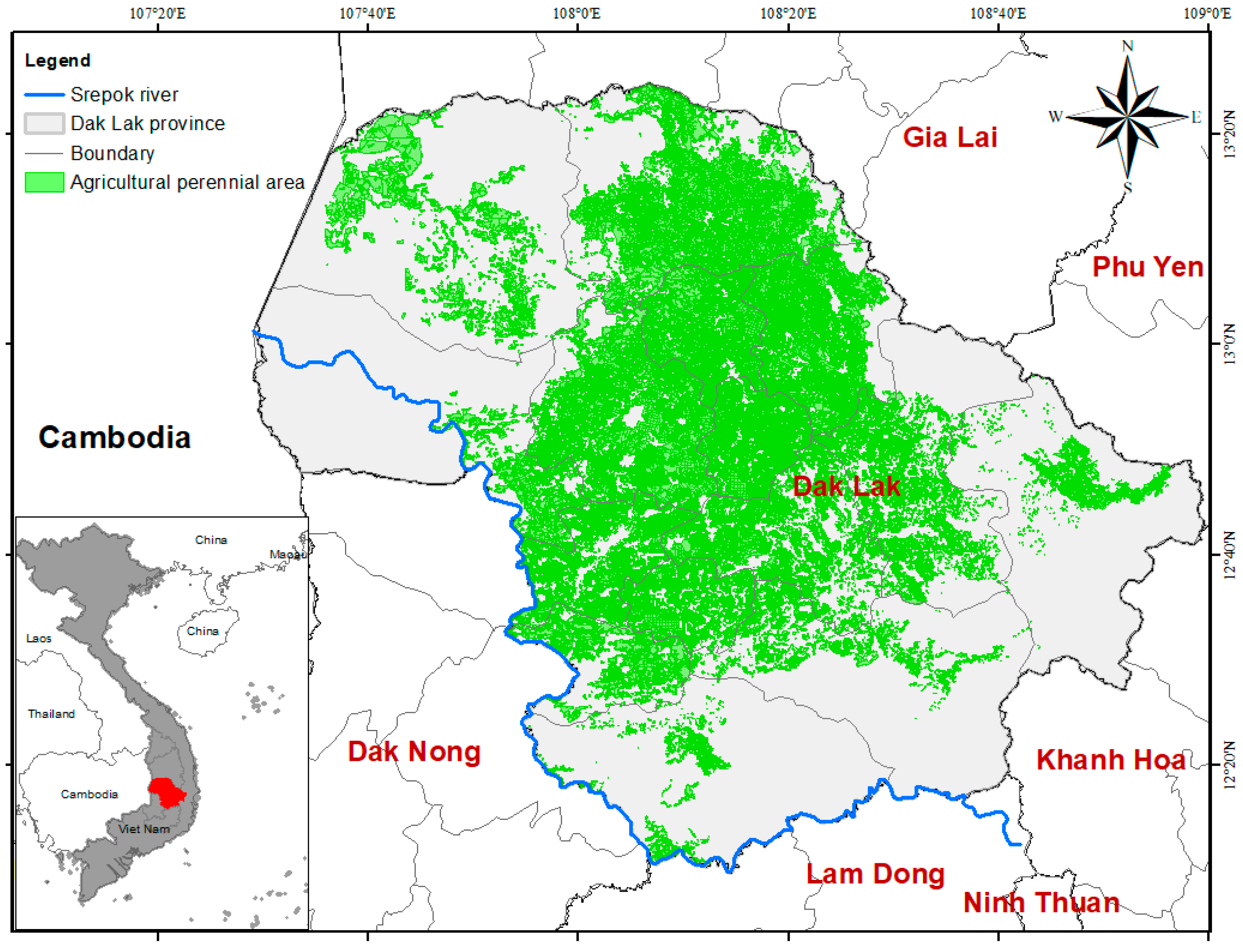
2.1. Study Area
2.2. Phenological Variables from Remote Sensing Time Series
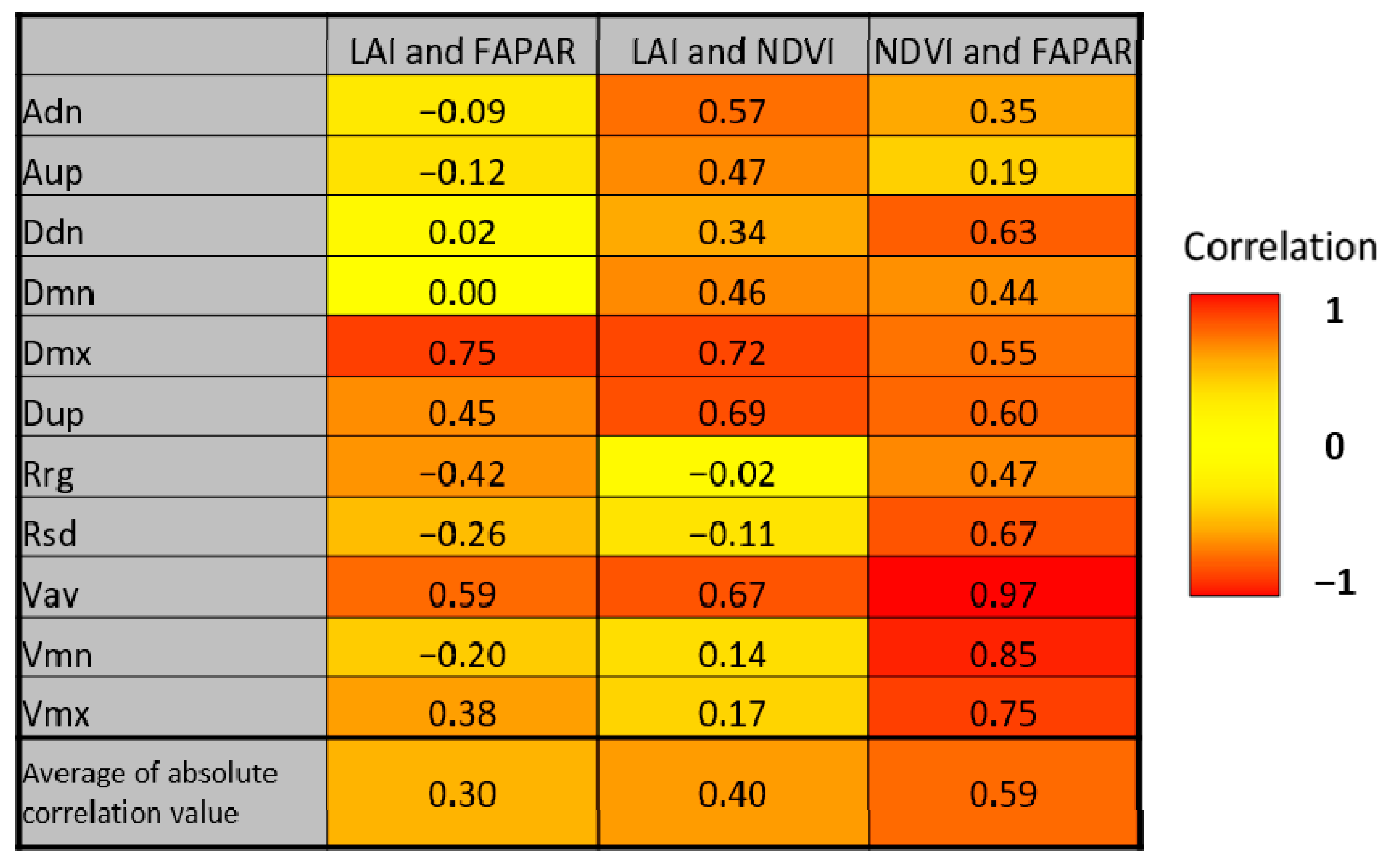
2.2.1. Vegetation Biophysical Variables
“The normalized difference vegetation index (NDVI) is an indicator of the greenness of the vegetation biomes”.(source: https://land.copernicus.eu/global/products/ndvi (accessed on 22 December 2021))
“The Leaf Area Index is defined as half the total area of green elements of the canopy per unit horizontal ground area. The satellite-derived value corresponds to the total green LAI of all the canopy layers, including the understory which may represent a very significant contribution, particularly for forests. Practically, the LAI quantifies the thickness of the vegetation cover.”(source: https://land.copernicus.eu/global/products/lai (accessed on 22 December 2021))
“The FAPAR quantifies the fraction of the solar radiation absorbed by live leaves for the photosynthesis activity. Then, it refers only to the green and alive elements of the canopy.”(source: https://land.copernicus.eu/global/products/FAPAR (accessed on 22 December 2021))
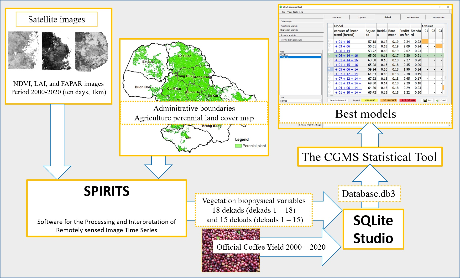
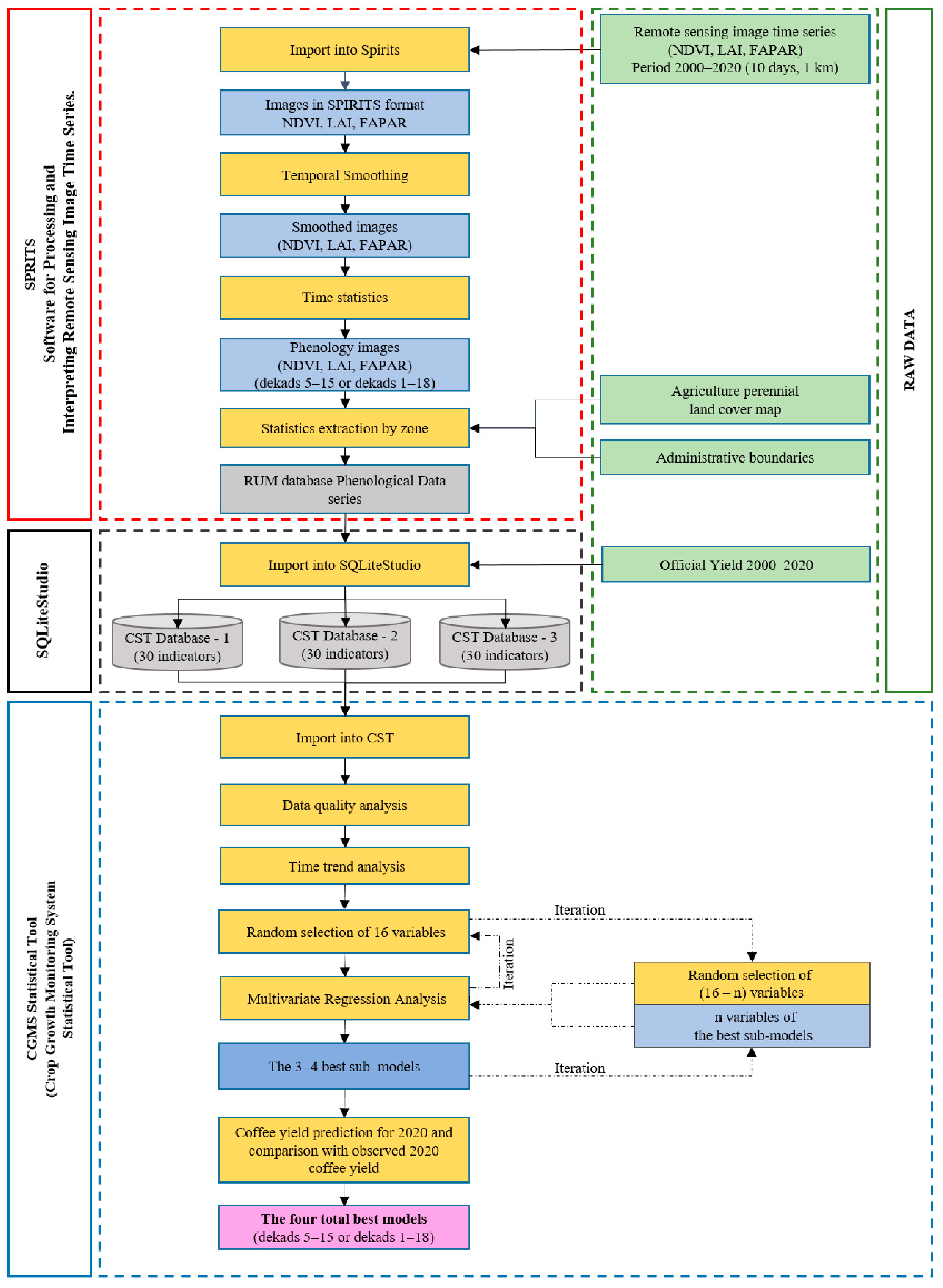
2.2.2. Processing of Satellite Images in SPIRITS Software
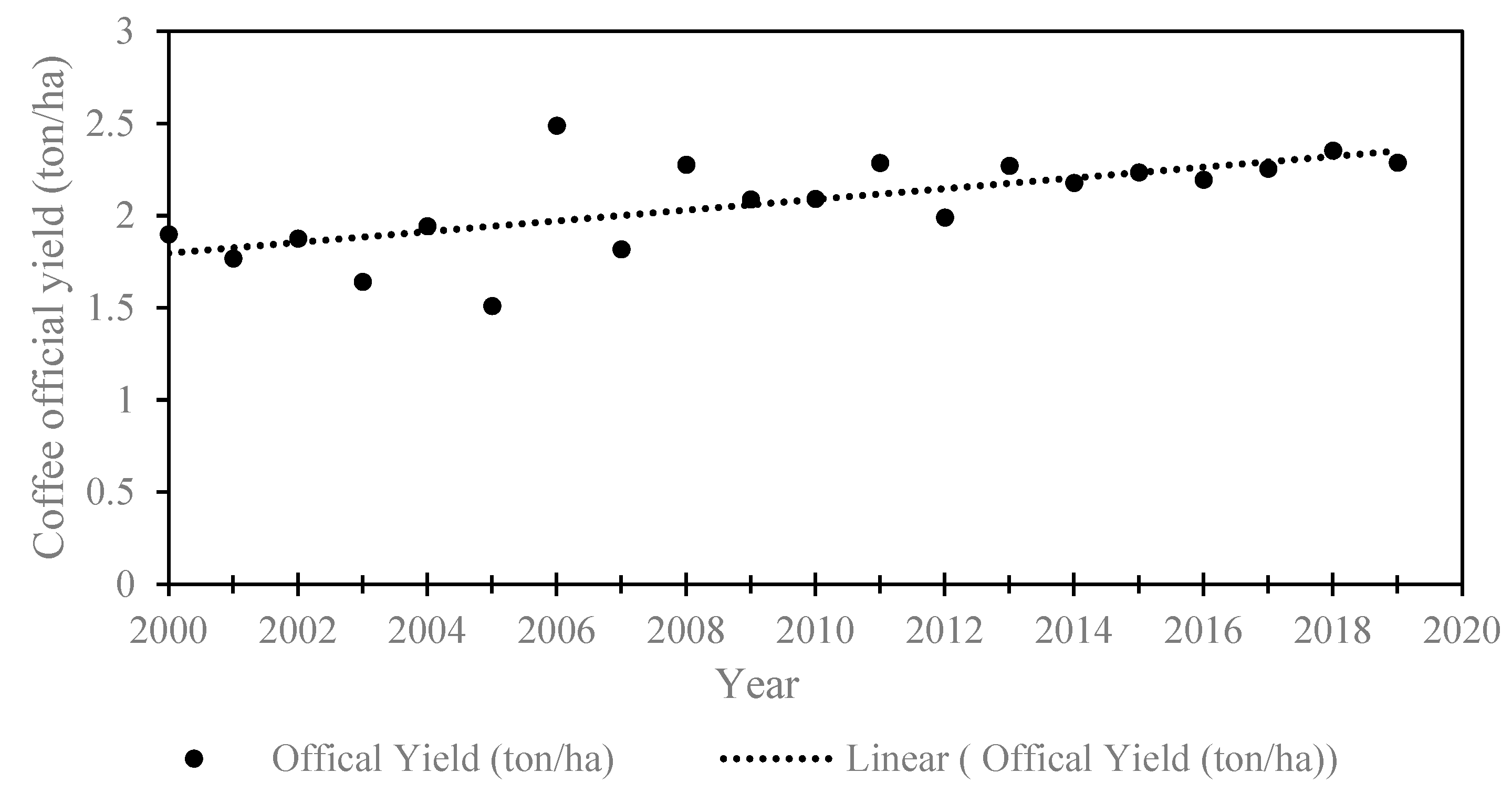
2.3. Official Coffee Yield Datasets
2.4. Crop Yield Forecasting Model in the CST Software
“CST takes the potential time trend into account by adding a term in the model that corresponds to that time trend, if applicable. To increase numerical precision, the regression coefficient for the linear time trend is for “year-offset” rather than “year” itself. The offset is fixed at 1965 by default in CST. Likewise, the regression coefficient for the quadratic time trend is for (year-offset)2.”[28]
3. Results
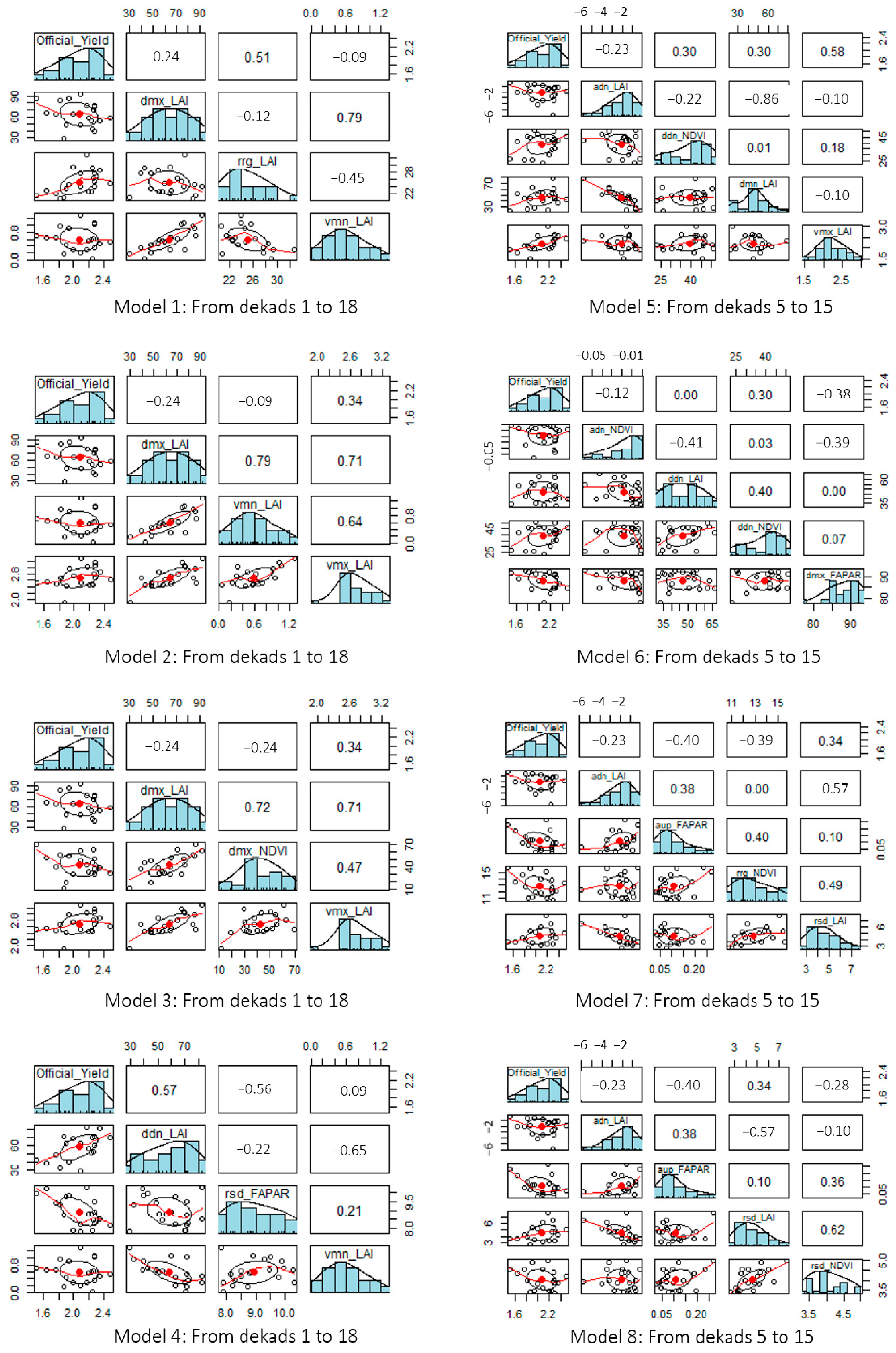
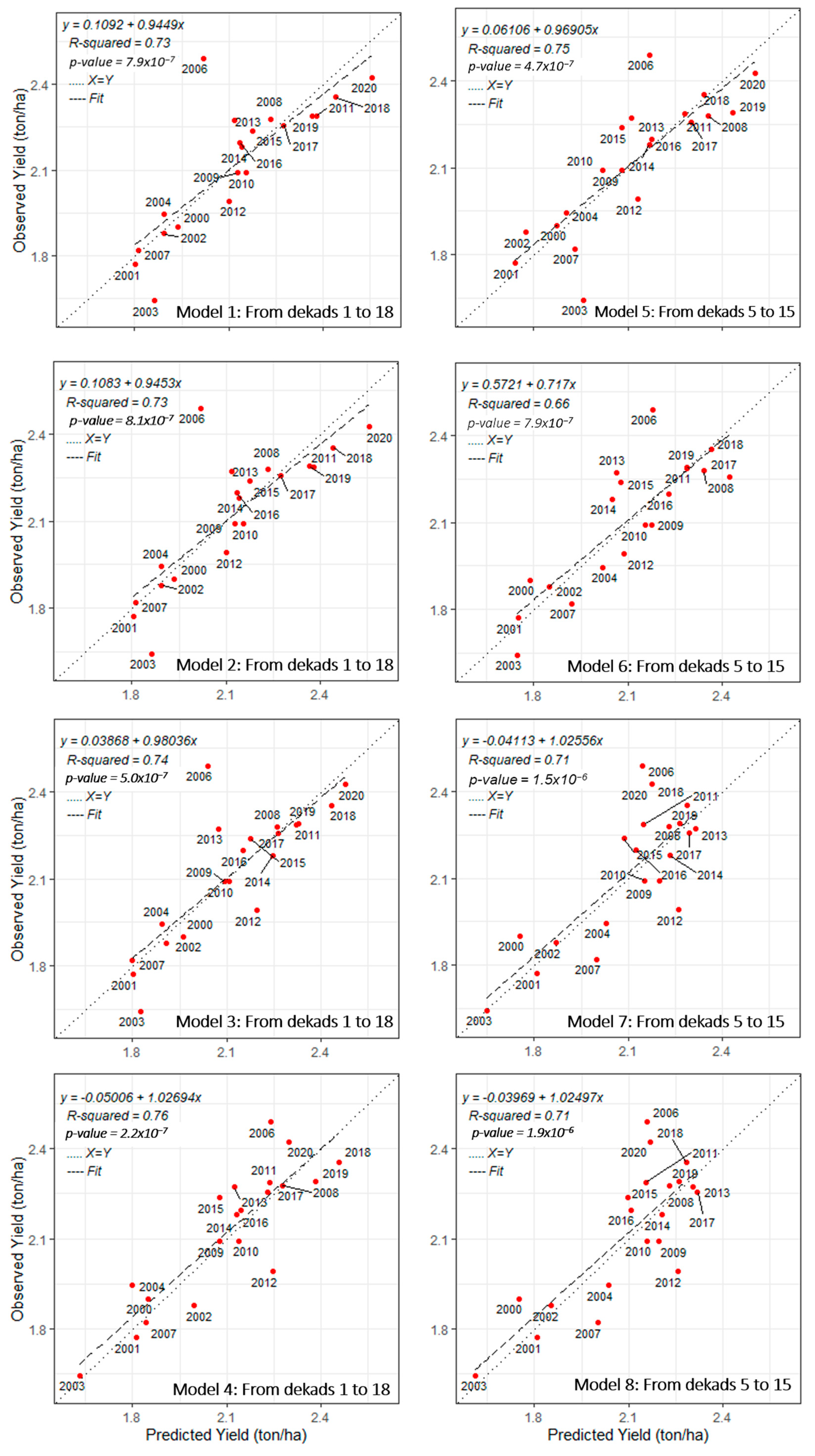
3.1. Model Performance
3.2. Coffee Yield Predictions for 2020
4. Discussion
5. Conclusions
Author Contributions
Funding
Data Availability Statement
Acknowledgments
Conflicts of Interest
References
- Ubilava, D. El Niño, La Niña, and World Coffee Price Dynamics. Agric. Econ. 2012, 43, 17–26. [Google Scholar] [CrossRef]
- Pohlan, J.; Janssens, M. Growth and Production of Coffee. In Soils, Plant Growth and Crop Production; Verheye, W.H., Ed.; Encyclopedia of Life: Oxford, UK, 2015. [Google Scholar]
- Kouadio, L.; Tixier, P.; Byrareddy, V.; Marcussen, T.; Mushtaq, S.; Rapidel, B.; Stone, R. Performance of a Process-Based Model for Predicting Robusta Coffee Yield at the Regional Scale in Vietnam. Ecol. Model. 2021, 443, 109469. [Google Scholar] [CrossRef]
- DaMatta, F.M.; Rahn, E.; Läderach, P.; Ghini, R.; Ramalho, J.C. Why Could the Coffee Crop Endure Climate Change and Global Warming to a Greater Extent than Previously Estimated? Clim. Chang. 2019, 152, 167–178. [Google Scholar] [CrossRef] [Green Version]
- Pham, Y.; Reardon-Smith, K.; Mushtaq, S.; Cockfield, G. The Impact of Climate Change and Variability on Coffee Production: A Systematic Review. Clim. Chang. 2019, 156, 609–630. [Google Scholar] [CrossRef]
- Piato, K.; Lefort, F.; Subía, C.; Caicedo, C.; Calderón, D.; Pico, J.; Norgrove, L. Effects of Shade Trees on Robusta Coffee Growth, Yield and Quality. A Meta-Analysis. Agron. Sustain. Dev. 2020, 40, 38. [Google Scholar] [CrossRef]
- USDA. Foreign Agricultural Service Volume of Coffee Exports from Vietnam from 2011 to 2021. Available online: https://www.statista.com/statistics/877329/vietnam-coffee-export-volume/ (accessed on 10 December 2021).
- ICO. Coffee Production Worldwide in 2020, by Leading Country. Available online: https://www.statista.com/statistics/277137/world-coffee-production-by-leading-countries/ (accessed on 10 December 2021).
- Thao, N.T.T.; Khoi, D.N.; Xuan, T.T.; Tychon, B. Assessment of Livelihood Vulnerability to Drought: A Case Study in Dak Nong Province, Vietnam. Int. J. Disaster Risk Sci. 2019, 10, 604–615. [Google Scholar] [CrossRef] [Green Version]
- Jayakumar, M.; Rajavel, M.; Surendran, U.; Gopinath, G.; Ramamoorthy, K. Impact of Climate Variability on Coffee Yield in India—with a Micro-Level Case Study Using Long-Term Coffee Yield Data of Humid Tropical Kerala. Clim. Chang. 2017, 145, 335–349. [Google Scholar] [CrossRef]
- Kath, J.; Byrareddy, V.M.; Craparo, A.; Nguyen-Huy, T.; Mushtaq, S.; Cao, L.; Bossolasco, L. Not so Robust: Robusta Coffee Production Is Highly Sensitive to Temperature. Glob. Chang. Biol. 2020, 26, 3677–3688. [Google Scholar] [CrossRef]
- Nguyen, D.Q.; Renwick, J.; Mcgregor, J. Variations of Surface Temperature and Rainfall in Vietnam from 1971 to 2010. Int. J. Climatol. 2014, 34, 249–264. [Google Scholar] [CrossRef]
- Van Viet, L. Development of a New ENSO Index to Assess the Effects of ENSO on Temperature over Southern Vietnam. Theor. Appl. Climatol. 2021, 144, 1119–1129. [Google Scholar] [CrossRef]
- Vo, T. Vietnam Coffee Annual 2020; USDA: Washington, DC, USA, 2021; Volume 2021. [Google Scholar]
- Gutierrez, A.P.; Villacorta, A.; Cure, J.R.; Ellis, C.K. Tritrophic Analysis of the Coffee (Coffea Arabica)—Coffee Berry Borer [Hypothenemus Hampei (Ferrari)]—Parasitoid System. An. Soc. Entomol. Bras. 1998, 27, 357–385. [Google Scholar] [CrossRef]
- Rodríguez, D.; Cure, J.R.; Cotes, J.M.; Gutierrez, A.P.; Cantor, F. A Coffee Agroecosystem Model: I. Growth and Development of the Coffee Plant. Ecol. Model. 2011, 222, 3626–3639. [Google Scholar] [CrossRef]
- Vezy, R.; le Maire, G.; Christina, M.; Georgiou, S.; Imbach, P.; Hidalgo, H.G.; Alfaro, E.J.; Blitz-Frayret, C.; Charbonnier, F.; Lehner, P.; et al. DynACof: A Process-Based Model to Study Growth, Yield and Ecosystem Services of Coffee Agroforestry Systems. Environ. Model. Softw. 2020, 124, 104609. [Google Scholar] [CrossRef] [Green Version]
- Van Oijen, M.; Dauzat, J.; Harmand, J.M.; Lawson, G.; Vaast, P. Coffee Agroforestry Systems in Central America: II. Development of a Simple Process-Based Model and Preliminary Results. Agrofor. Syst. 2010, 80, 361–378. [Google Scholar] [CrossRef]
- Rahn, E.; Vaast, P.; Läderach, P.; van Asten, P.; Jassogne, L.; Ghazoul, J. Exploring Adaptation Strategies of Coffee Production to Climate Change Using a Process-Based Model. Ecol. Model. 2018, 371, 76–89. [Google Scholar] [CrossRef]
- Ovalle-Rivera, O.; Van Oijen, M.; Läderach, P.; Roupsard, O.; de Melo Virginio Filho, E.; Barrios, M.; Rapidel, B. Assessing the Accuracy and Robustness of a Process-Based Model for Coffee Agroforestry Systems in Central America. Agrofor. Syst. 2020, 94, 2033–2051. [Google Scholar] [CrossRef]
- Kouadio, L.; Deo, R.C.; Byrareddy, V.; Adamowski, J.F.; Mushtaq, S.; Phuong Nguyen, V. Artificial Intelligence Approach for the Prediction of Robusta Coffee Yield Using Soil Fertility Properties. Comput. Electron. Agric. 2018, 155, 324–338. [Google Scholar] [CrossRef]
- Molina, A.L.V.; Peralta, V.P.P.; Orozco, A.B.P.; Iglesias, M.I.O.; Guerrero, E.G. Calibration of the Aquacrop Model in Special Coffee (Coffea Arabica) Crops in the Sierra Nevada of Santa Marta, Colombia. J. Agron. 2018, 17, 241–250. [Google Scholar] [CrossRef] [Green Version]
- Fall, C.M.N.; Lavaysse, C.; Kerdiles, H.; Dramé, M.S.; Roudier, P.; Gaye, A.T. Performance of Dry and Wet Spells Combined with Remote Sensing Indicators for Crop Yield Prediction in Senegal. Clim. Risk Manag. 2021, 33, 100331. [Google Scholar] [CrossRef]
- Tebaldi, C.; Lobell, D.B. Towards Probabilistic Projections of Climate Change Impacts on Global Crop Yields. Geophys. Res. Lett. 2008, 35, 2–7. [Google Scholar] [CrossRef]
- Laudien, R.; Schauberger, B.; Makowski, D.; Gornott, C. Robustly Forecasting Maize Yields in Tanzania Based on Climatic Predictors. Sci. Rep. 2020, 10, 19650. [Google Scholar] [CrossRef]
- Nain, A.S.; Dadhwal, V.K.; Singh, T.P. Use of CERES-Wheat Model for Wheat Yield Forecast in Central Indo-Gangetic Plains of India. J. Agric. Sci. 2004, 142, 59–70. [Google Scholar] [CrossRef]
- Lobell, D.B.; Burke, M.B. On the Use of Statistical Models to Predict Crop Yield Responses to Climate Change. Agric. For. Meteorol. 2010, 150, 1443–1452. [Google Scholar] [CrossRef]
- Goedhart, P.W.; Hoek, S.B.; Boogaard, H.L. The CGMS Statistical Tool; Contributions by 2019; European Commission: Ispra, Italy, 2019. [Google Scholar]
- Kerdiles, H.; Rembold, F.; Leo, O.; Boogaard, H.; Hoek, S. CST, a Freeware for Predicting Crop Yield from Remote Sensing or Crop Model Indicators: Illustration with RSA and Ethiopia. In Proceedings of the 2017 6th International Conference on Agro-Geoinformatics, Fairfax, VA, USA, 7–10 August 2017. [Google Scholar] [CrossRef]
- Qing, H.; Fei, T.; Jianqiang, R.; Wenbin, W.; Dandan, L.; Hui, D. The Application of China-CGMS in the Main Crop Growth Monitoring in Northeast China. In Proceedings of the 2012 First International Conference on Agro- Geoinformatics (Agro-Geoinformatics), Shanghai, China, 2–4 August 2012; pp. 1–4. [Google Scholar]
- Rembold, F.; Meroni, M.; Urbano, F.; Royer, A.; Atzberger, C.; Lemoine, G.; Eerens, H.; Haesen, D. Remote Sensing Time Series Analysis for Crop Monitoring with the SPIRITS Software: New Functionalities and Use Examples. Front. Environ. Sci. 2015, 3, 46. [Google Scholar] [CrossRef] [Green Version]
- Balaghi, R.; Badjeck, M.C.; Bakari, D.; De Pauw, E.D.; De Wit, A.; Defourny, P.; Donato, S.; Gommes, R.; Jlibene, M.; Ravelo, A.C.; et al. Managing Climatic Risks for Enhanced Food Security: Key Information Capabilities. Procedia Environ. Sci. 2010, 1, 313–323. [Google Scholar] [CrossRef] [Green Version]
- De Wit, A.; Duveiller, G.; Defourny, P. Estimating Regional Winter Wheat Yield with WOFOST through the Assimilation of Green Area Index Retrieved from MODIS Observations. Agric. For. Meteorol. 2012, 164, 39–52. [Google Scholar] [CrossRef]
- Araya, S.; Ostendorf, B.; Lyle, G.; Lewis, M. Remote Sensing Derived Phenological Metrics to Assess the Spatio-Temporal Growth Variability in Cropping Fields. Adv. Remote Sens. 2017, 06, 212–228. [Google Scholar] [CrossRef] [Green Version]
- López-Lozano, R.; Duveiller, G.; Seguini, L.; Meroni, M.; García-Condado, S.; Hooker, J.; Leo, O.; Baruth, B. Towards Regional Grain Yield Forecasting with 1km-Resolution EO Biophysical Products: Strengths and Limitations at Pan-European Level. Agric. For. Meteorol. 2015, 206, 12–32. [Google Scholar] [CrossRef]
- Bernardes, T.; Moreira, M.A.; Adami, M.; Giarolla, A.; Rudorff, B.F.T. Monitoring Biennial Bearing Effect on Coffee Yield Using MODIS Remote Sensing Imagery. Remote Sens. 2012, 4, 2492–2509. [Google Scholar] [CrossRef] [Green Version]
- Nogueira, S.M.C.; Moreira, M.A.; Volpato, M.M.L. Relationship between coffee crop productivity and vegetation indexes derived from oli/landsat-8 sensor data with and without topographic correction. Int. Braz. Assoc. Agric. Eng. 2018, 38, 387–394. [Google Scholar] [CrossRef]
- DakLak Provincial People’s Committee. Available online: https://daklak.gov.vn/web/english/about-daklak (accessed on 4 April 2022).
- CCAFS-SEA. The Drought Crisis in the Central Highlands of Vietnam—Assessment Report; CGIAR Research Program on Climate Change, Agriculture and Food Security (CCAFS): Hanoi, Vietnam, 2016. [Google Scholar]
- DakLak Statistical Office. DakLak Statistical Yearbook 2020; DakLak Statistical Office: DakLak, Vietnam, 2021. [Google Scholar]
- Huong, N.T.; Anh, L.H. Factors Affecting the Technical Efficiency of Coffee Producers—Case Study in Dak Lak Province, Vietnam. Int. J. Econ. Commer. Manag. 2019, VII, 535–543. [Google Scholar]
- Byrareddy, V.; Kouadio, L.; Kath, J.; Mushtaq, S.; Rafiei, V.; Scobie, M.; Stone, R. Win-Win: Improved Irrigation Management Saves Water and Increases Yield for Robusta Coffee Farms in Vietnam. Agric. Water Manag. 2020, 241, 106350. [Google Scholar] [CrossRef]
- Titus, A.; Pereira, G.N. Water Use Efficiency for Robusta Coffee. Available online: https://ecofriendlycoffee.org/water-use-efficiency-robusta-coffee/ (accessed on 17 December 2021).
- Eerens, H.; Dominique, H. Software for the Processing and Interpretation of Remotely Sensed Image Time Series; User’s Manual Version 1.5.2—February 2018; VITO, EU Joint Research Center: Ispra, Italy, 2018. [Google Scholar]
- Swets, D.; Reed, B.C.; Rowland, J.; Marko, S.E. A Weighted Least-Squares Approach to Temporal NDVI Smoothing. In Proceedings of the From Image to Information: 1999 ASPRS Annual Conference, Portland, Oregon, 17–21 May 1999. [Google Scholar]
- DakLak Statistical Office. DakLak Statistical Yearbook 2009; DakLak Statistical Office: DakLak, Vietnam, 2010. [Google Scholar]
- DakLak Statistical Office. DakLak Statistical Yearbook 2014; DakLak Statistical Office: DakLak, Vietnam, 2015. [Google Scholar]
- DakLak Statistical Office. DakLak Statistical Yearbook 2018; DakLak Statistical Office: DakLak, Vietnam, 2019. [Google Scholar]


| Remote Sensing Vegetation Biophysical Products | Definition | Period |
|---|---|---|
| FAPAR | Fraction of absorbed photosynthetically active radiation | 2000–2020 |
| LAI | Leaf area index | 2000–2020 |
| NDVI | Normalized difference vegetation index | 2000–2020 |
| No. | Variable | Definition | Dekads |
|---|---|---|---|
| 1 | vav | Average value (or mean) | 5–15; 1–18 |
| 2 | vmn | Minimum value | 5–15; 1–18 |
| 3 | vmx | Maximum value | 5–15; 1–18 |
| 4 | aup | Largest increase between subsequent periods | 5–15; 1–18 |
| 5 | adn | Largest decrease between subsequent periods | 5–15; 1–18 |
| 6 | rsd | Relative standard deviation (with N as denominator, not N − 1) | 5–15; 1–18 |
| 7 | rrg | Relative range (maximum–minimum) | 5–15; 1–18 |
| 8 | dmn | Relative date of (first) minimum value | 5–15; 1–18 |
| 9 | dmx | Relative date of (last) maximum value | 5–15; 1–18 |
| 10 | dup | Relative date of (first) largest increase | 5–15; 1–18 |
| 11 | ddn | Relative date of (last) largest decrease | 5–15; 1–18 |
| Parameter | Estimate | s.e. | t Value | RMSEp | RRMSE | R2 | Adj.R2 | MAPE | RSD | |
|---|---|---|---|---|---|---|---|---|---|---|
| (ton/ha) | (%) | (%) | (%) | (%) | (ton/ha) | |||||
| Model 0 No dekad | Constant | 0.774 | 0.342 | 2.26 | 0.202 | 9.7 | 41.8 | 4.3 | 0.197 | |
| Time trend (linear) | 0.029 | 7.63 × 10⁻³ | 3.83 | 44.8 | ||||||
| Model 1 Dekads 1–18 | Constant | 0.496 | 0.361 | 1.37 | 0.155 | 7.5 | 64.2 | 4.3 | 0.154 | |
| Time trend (linear) | 0.018 | 7.30 × 10⁻³ | 2.46 | |||||||
| dmx-LAI | −0.013 | 3.84 × 10⁻³ | −3.48 | 71.7 | ||||||
| rrg-LAI | 0.048 | 0.016 | 2.91 | |||||||
| vmn-LAI | 0.727 | 0.231 | 3.14 | |||||||
| Model 2 Dekads 1–18 | Constant | 0.494 | 0.362 | 1.37 | 0.155 | 7.5 | 64.5 | 4.3 | 0.154 | |
| Time trend (linear) | 0.018 | 7.30 × 10⁻³ | 2.47 | |||||||
| dmx-LAI | −0.013 | 3.85 × 10⁻³ | −3.47 | 71.7 | ||||||
| vmn-LAI | 0.155 | 0.186 | 0.83 | |||||||
| vmx-LAI | 0.572 | 0.197 | 2.91 | |||||||
| Model 3 Dekads 1–18 | Constant | 0.415 | 0.346 | 1.2 | 0.155 | 7.5 | 64.9 | 3.9 | 0.153 | |
| Time trend (linear) | 0.019 | 7.39 × 10⁻³ | 2.56 | |||||||
| dmx-LAI | −8.74 × 10⁻³ | 4.27 × 10⁻³ | −2.05 | 72.3 | ||||||
| dmx-NDVI | −3.58 × 10⁻³ | 3.53 × 10⁻³ | −1.01 | |||||||
| vmx-LAI | 0.567 | 0.194 | 2.93 | |||||||
| Model 4 Dekads 1–18 | Constant | 1.708 | 0.592 | 2.88 | 0.158 | 7.6 | 68.8 | 4.7 | 0.144 | |
| Time trend linear | 0.013 | 6.79 × 10⁻³ | 1.92 | |||||||
| ddn-LAI | 0.011 | 3.00 × 10⁻³ | 3.65 | 75.4 | ||||||
| rsd-FAPAR | −0.119 | 0.046 | −2.56 | |||||||
| vmn-LAI | 0.35 | 0.139 | 2.52 | |||||||
| Model 5 Dekads 5–15 | Constant | −0.344 | 0.412 | −0.84 | 0.174 | 8.4 | 62.8 | 4.7 | 0.157 | |
| Time trend (linear) | 0.015 | 7.86 × 10⁻³ | 1.85 | |||||||
| adn-LAI | 0.152 | 0.062 | 2.43 | 72.6 | ||||||
| ddn-NDVI | 9.96 × 10⁻³ | 4.54 × 10⁻³ | 2.19 | |||||||
| dmn-LAI | 0.019 | 6.24 × 10⁻³ | 2.97 | |||||||
| vmx-LAI | 0.382 | 0.144 | 2.66 | |||||||
| Model 6 Dekads 5–15 | Constant | 3.218 | 0.972 | 3.31 | 0.177 | 8.5 | 67.6 | 5.6 | 0.147 | |
| Time trend (linear) | 0.025 | 6.10 × 10⁻³ | 4.13 | |||||||
| adn-NDVI | −9.122 | 2.602 | −3.51 | 76.1 | ||||||
| ddn-LAI | −0.01 | 4.03 × 10⁻³ | −2.55 | |||||||
| ddn-NDVI | 0.014 | 4.44 × 10⁻³ | 3.05 | |||||||
| dmx-FAPAR | −0.028 | 9.69 × 10⁻³ | −2.9 | |||||||
| Model 7 Dekads 5–15 | Constant | 1.917 | 0.738 | 2.6 | 0.178 | 8.6 | 63.6 | 5.0 | 0.156 | |
| Time trend (linear) | 0.015 | 9.21 × 10⁻³ | 1.67 | |||||||
| adn-LAI | 0.081 | 0.039 | 2.06 | 73.2 | ||||||
| aup-FAPAR | −1.74 | 0.673 | −2.58 | |||||||
| rrg-NDVI | −0.067 | 0.043 | −1.55 | |||||||
| rsd-LAI | 0.152 | 0.055 | 2.79 | |||||||
| Model 8 Dekads 5–15 | Constant | 1.878 | 0.754 | 2.49 | 0.178 | 8.6 | 62.9 | 5.3 | 0.157 | |
| Time trend (linear) | 0.016 | 9.36 × 10⁻³ | 1.69 | |||||||
| adn-LAI | 0.081 | 0.04 | 2.04 | 72.7 | ||||||
| aup-FAPAR | −1.806 | 0.67 | −2.7 | |||||||
| rsd-LAI | 0.165 | 0.063 | 2.6 | |||||||
| rsd-NDVI | −0.221 | 0.151 | −1.46 |
| Predicted Yield (ton/ha) | Official Yield (ton/ha) | Residual (ton/ha) | Percentage Residual (%) | |
|---|---|---|---|---|
| Model 1 | 2.558 | 2.424 | 0.134 | 5.5 |
| Model 2 | 2.558 | 2.424 | 0.134 | 5.5 |
| Model 3 | 2.478 | 2.424 | 0.054 | 2.2 |
| Model 4 | 2.298 | 2.424 | −0.126 | −5.2 |
| Model 5 | 2.506 | 2.424 | 0.082 | 3.4 |
| Model 6 | 2.995 | 2.424 | 0.571 | 23.6 |
| Model 7 | 2.176 | 2.424 | −0.248 | −10.2 |
| Model 8 | 2.171 | 2.424 | −0.253 | −10.4 |
Publisher’s Note: MDPI stays neutral with regard to jurisdictional claims in published maps and institutional affiliations. |
© 2022 by the authors. Licensee MDPI, Basel, Switzerland. This article is an open access article distributed under the terms and conditions of the Creative Commons Attribution (CC BY) license (https://creativecommons.org/licenses/by/4.0/).
Share and Cite
Thao, N.T.T.; Khoi, D.N.; Denis, A.; Viet, L.V.; Wellens, J.; Tychon, B. Early Prediction of Coffee Yield in the Central Highlands of Vietnam Using a Statistical Approach and Satellite Remote Sensing Vegetation Biophysical Variables. Remote Sens. 2022, 14, 2975. https://doi.org/10.3390/rs14132975
Thao NTT, Khoi DN, Denis A, Viet LV, Wellens J, Tychon B. Early Prediction of Coffee Yield in the Central Highlands of Vietnam Using a Statistical Approach and Satellite Remote Sensing Vegetation Biophysical Variables. Remote Sensing. 2022; 14(13):2975. https://doi.org/10.3390/rs14132975
Chicago/Turabian StyleThao, Nguyen Thi Thanh, Dao Nguyen Khoi, Antoine Denis, Luong Van Viet, Joost Wellens, and Bernard Tychon. 2022. "Early Prediction of Coffee Yield in the Central Highlands of Vietnam Using a Statistical Approach and Satellite Remote Sensing Vegetation Biophysical Variables" Remote Sensing 14, no. 13: 2975. https://doi.org/10.3390/rs14132975
APA StyleThao, N. T. T., Khoi, D. N., Denis, A., Viet, L. V., Wellens, J., & Tychon, B. (2022). Early Prediction of Coffee Yield in the Central Highlands of Vietnam Using a Statistical Approach and Satellite Remote Sensing Vegetation Biophysical Variables. Remote Sensing, 14(13), 2975. https://doi.org/10.3390/rs14132975