Abstract
High-resolution surface freeze/thaw (F/T) information is valuable for hydrological, frost creep and gelifluction/solifluction, and climate prediction studies. Currently, large-scale, high-resolution F/T detection is restricted by low spatial resolution of passive microwave remote sensing sensors or low temporal resolution of synthetic aperture radar (SAR) data. In this study, we propose a new method for detecting daily land surface F/T state at 1 km spatial resolution by combining the Sentinel-1 radar and the Advanced Microwave Scanning Radiometer 2 (AMSR2) with leaf area index (LAI) data. A non-linear relationship is established between the 1 km F/T index from Sentinel-1 with 1 km F/T index from AMSR2 (FTI) and 1 km LAI data. The 1 km FTI is a disaggregation of the 25 km FTI obtained from AMSR2. This non-linear relationship is then applied to daily 1 km FTI and LAI data to predict the 1 km daily F/T index, based on which the F/T status is detected with grid-cell-based F/T thresholds. The overall accuracy of this daily 1 km F/T is more than 88.1% when evaluated with the in situ 5 cm soil temperature over China and Canada. This study is valuable for detecting daily, high-resolution F/T status and is helpful for studies related to disaster and climate prediction.
1. Introduction
Approximately 50 million square kilometers of the land surface experiences soil freezing and thawing [1]. Part of this surface exhibits spatially discontinuous soil freezing and thawing changes due to the heterogeneity of topography, land cover, subsurface properties, snow cover, and other factors. The spatial and temporal change information of land surface freeze/thaw (F/T) is essential for hydrological, climatic, topographic deformation, and ecosystem processes [2,3,4,5,6]. The land surface F/T that occurs in permafrost regions increases emissions of carbon and nitrogen [7,8,9,10] and leads to uncertainties in climate change predictions [11]. Permafrost degradation in high mountains could lead to disasters, such as rock and ice avalanches [12]. High-resolution mapping of permafrost covering high-altitude areas is important for infrastructure planning [13]. High-resolution monitoring of surface F/T states is important for various research areas, particularly disasters, such as frost creep and gelifluction/solifluction [14], spring floods, and climate prediction [15,16]. Remotely sensed satellite data are efficient for detecting land surface F/T states at global and regional scales; satellite microwave remote sensing at long wavelengths is well suited for detecting the soil F/T state because of the ability to penetrate into the soil medium [17,18] and the high contrast in permittivity between liquid water and ice [19]. Active and passive microwave data have been widely used to detect land surface F/T in recent years. Several global and regional microwave surface F/T products have been produced with active and passive microwave sensors, such as the Advanced Microwave Scanning Radiometer 2 (AMSR2) [20,21], Soil Moisture and Ocean Salinity (SMOS) [22], Soil Moisture Active Passive (SMAP) [23], the Aquarius L-band radiometer [24], and the advanced scatterometer (ASCAT) [25]. All these F/T products detect the land surface F/T state at spatial resolutions from 25 km to 36 km, which cannot accurately describe the surface F/T process within heterogeneous pixels and does not satisfy the requirements of many applications, e.g., frost creep and gelifluction/solifluction and flood disaster monitoring at regional scales. The scattering properties of synthetic aperture radar (SAR) data, such as scattering type (surface, double-bounce, and volume scattering) and entropy, in different land covers (such as forest or non-forest, snow-covered or snow-free), land F/T status had significant seasonal changes and could be used for mapping land cover types and surficial geocryological characteristics of the permafrost active layer [26,27]. The obviously seasonal variations of the backscattered signal has been used to detect land surface F/T. Sentinel-1 (S1) satellite data, which can provide free high-resolution SAR data since 2015 and have high data volume coverage over study areas in this study, have been successfully used to detect land surface F/T [28,29,30,31,32]. However, the temporal resolution of Sentinel-1 depends on the geographical location. For example, Sentinel-1 is available daily in northern Europe but only once every 12 days in northeastern China. A high-resolution F/T detection algorithm is required to detect daily high-resolution surface F/T states over some areas where S1 data are not available daily and meet the demand for many regional frost creep and gelifluction/solifluction and climate change studies.
Some studies have developed F/T detection algorithm in which high-resolution optical/thermal data were used to downscale passive microwave data. Kou et al. [33] detected the land surface F/T state at 0.05° with the discriminant function algorithm (DFA) [34] from brightness temperature (Tb), which was downscaled by blending the land temperature data using a Bayesian maximum entropy method. Zhao et al. [35] established a relationship between the passive microwave F/T index (FTI) and thermal infrared observations to monitor high spatial resolution surface F/T states at 0.05°. However, these studies mainly concentrated on the Tibetan Plateau area by combining passive microwave and thermal infrared data. Additionally, using these methods might reduce the accuracy of passive microwave soil F/T detection [35] due to the different depths of F/T represented by passive microwave and thermal infrared.
Currently, there are a few studies regarding the detection of the F/T state that combine active and passive microwave satellite data. Zhong et al. [36] estimated more accurately F/T onsets by using a machine learning approach of combination SMAP and ASCAT. This study revealed the possibility of detecting F/T state by combing active and passive microwave remote sensing. The combination of passive and active data provides a potential means for downscaling soil moisture estimates to a finer spatial resolution [37,38,39]. The soil dielectric constant is highly dependent on the liquid water content; the higher the amount of free liquid water is, the higher the dielectric constant. For low dielectric constant values (dry or frozen soil), the backscattered signal from the soil surface is at its minimum, and the soil surface emission is at its maximum. Many methods, such as the Tb-based downscaling method [39], soil moisture-based downscaling method [37], and change detection method [40], have successfully estimated soil moisture at high spatial resolution by combining active and passive data. Surface F/T detection relies on observing changes in soil dielectric properties rather than the absolute value.
In this work, we demonstrate the feasibility of high spatial resolution surface F/T state determination by a combination of active and passive microwave data over four test regions located in China and Canada. The objectives of the study are to detect the daily land surface F/T state at a 1 km spatial resolution and to propose a new approach for detecting the F/T state combining radar and passive remote sensing data. The advanced integral equation method (AIEM) microwave emission and scattering model incorporating a dielectric constant of F/T soil is used to study the behavior of the radar and passive signals from thawed to frozen. Finally, a new approach is demonstrated for the detection of the surface F/T state at high spatial and temporal resolutions using Sentinel-1 and AMSR2 data by incorporating leaf area index (LAI) data. In Section 2, the study area and data used in this study are briefly described. In Section 3, a detailed description of our new algorithm development is presented. In Section 4 and Section 5, the results and discussion are given, followed by the conclusion in Section 6.
2. Materials
The dataset used consists of in situ data, Sentinel-1 SAR data, AMSR2 Tb data and auxiliary data. The auxiliary data include the ERA5-land reanalysis dataset and LAI data. The in situ soil moisture and temperature network located in China and Canada (Figure 1) was used to validate the accuracies of the F/T detection results.
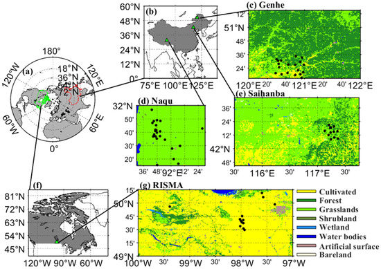
Figure 1.
Study area in Northern Hemisphere (a). Land cover map and distribution of in situ sites over the Genhe watershed (c), Saihanba (e), and Naqu (d) in China (b), and the RISMA network (g) in Canada (f).
2.1. In Situ Data
For the purposes of this study, data from four areas with distributed near-surface soil moisture and a temperature observation network could be obtained. Three in situ soil moisture and temperature observation networks, including the Genhe watershed, Saihanba, and Naqu, are located in China (Figure 1c–e), and another in situ soil moisture and temperature observation network, i.e., Real-time In Situ Monitoring for Agriculture (RISMA) network, located in Canada (Figure 1g). Each study area is affected by seasonal soil F/T and located within one Sentinel-1 image.
Genhe watershed study area is located in the northeast of China (50.25~51.25°N, 120~122°E). The prominent land cover types in the Genhe watershed, which has a combination of a cold and humid temperate climate and a continental monsoon climate, are forest, grassland, and cultivated land. The contents of clay and sand in soil over Genhe watershed are 36–52% and 3–29%, respectively, and the elevation ranges from 500 to 1420 m. The Genhe watershed is widely covered with permafrost. A soil temperature and moisture observation network has been established over the Genhe watershed since October 2013 [41,42]. Saihanba study area is located in the north of China (41.75~42.75°N, 115.5~117.75°E). Saihanba, with semi-arid and semi-humid climates, is mainly covered with forest and grassland with elevations ranging from 700 to 2000 m. The contents of clay and sand in soil over Saihanba are 9% and 79%, respectively. Seasonal frozen soil is widely distributed here. A soil moisture and temperature observation network has been established to measure data at depths of 5 cm and 10 cm since August 2018 over Saihanba [41]. Naqu, with a semiarid climate, is located in the central Qinghai-Tibetan Plateau and is distributed with permafrost (31.25~32°N, 91.5~92.5°E). The contents of clay and sand in soil over Naqu are 20% and 66%, respectively. With elevations ranging from 4280 to 5900, Naqu is mainly covered with alpine meadows. The in situ soil temperature at a depth of 5 cm was obtained from a multiscale soil moisture and temperature monitoring network [43]. The RISMA soil moisture and temperature network used in this study is located in Manitoba, Canada, covered with cultivated land and forest [44]. The contents of clay and sand in soil over RISMA are 9–70% and 3–90%, respectively. This RISMA network was established since 2011. The soil sensors measured the real dielectric permittivity, soil moisture, and soil temperature using Stevens Hydra Probe sensors at surface (0–5 cm), 5 cm, 20 cm, 50 cm, and 100 cm depths. Three hydra probe sensors were installed at each depth. Soil temperature data at a depth of 5 cm with an hour interval are downloaded from https://ismn.geo.tuwien.ac.at/en/and used in this study. RISMA has a cold climate and elevation ranging from 130 to 720 m. The RISMA study area (49~50.25°N, −100~−97°E) in this study includes the Manitoba RISMA network.
Taking into account the available time periods of the various soil moisture and temperature observation networks and the auxiliary data, a total of 19, 16, 23, and 13 ground sites from the Genhe watershed from June 2017 to May 2019, from Saihanba from August 2018 to December 2019, and from Naqu and RISMA from January 2018 to December 2019 were used in this study. Short descriptions of the in situ sites from the four study areas are given in Table 1. Figure 1c–e, and Figure 1g show the land cover map and distribution of in situ stations of the Genhe watershed, Naqu, Saihanba, and RISMA. The GlobeLand30–2010 land cover map provided by the National Geomatics Center of China was used here, and the land cover map was produced by integrating pixel- and object-based methods with knowledge and over 10,000 Landsat satellite images with more than 80% overall accuracy [45] (http://www.webmap.cn/mapDataAction.do?method=globalLandCover, accessed on 5 December 2021)

Table 1.
Coordinates and land cover type of the in situ sites.
2.2. Satellite Data
Sentinel-1 comprises a constellation of two polar-orbiting satellites (Sentinel-1A (S1A) and -1B (S1B)), performing the C-band (5.406 GHz) synthetic aperture radar (SAR) imaging. S1A and S1B were launched in April 2014 and April 2016, respectively. Sentinel-1 data products are available from https://scihub.copernicus.eu/dhus/#/home, accessed on 20 December 2021. Only S1B has acquired data over the Genhe watershed and RISMA, and only S1A has acquired data over Naqu. Both S1A and S1B acquired data over Saihanba, but to match the descending AMSR2 data with overpass time at 1:30 am, S1B data with overpass time at 22:20 pm were used. The revisit frequency of S1 data over the four study areas is as long as 12 days. A short description of the S1 data of the four study areas is given in Table 2.

Table 2.
Detailed information on S1 data over the four study areas. Number means the number of S1 SAR images during the time period.
The S1 SAR data used in this study are interferometric wide swath mode (IW) images in both VV and VH polarizations that were generated from the Level-1 ground range detected (GRD) product. First, the S1 SAR images were preprocessed. The preprocessing steps include multilooking processing, radiometric correction, filtering, and geometric correction using Shuttle Radar Topography Mission (SRTM) digital elevation model (DEM) data. Then, the image pixel values were converted to backscatter coefficients (). The backscatter coefficients obtained from different incidence angles () were normalized to 40° () according to the square cosine correction equation [46,47]:
Finally, the spatial resolution of the preprocessed S1 data was resampled from 20 m to 1 km using the average sampling method.
The passive microwave data used in this study are AMSR2 L3 Tb (6.925 GHz and 36.5 GHz) with a spatial resolution of 0.25° provided by the Japan Aerospace Exploration Agency (JAXA) (https://gportal.jaxa.jp/gpr/information/product, accessed on 20 December 2021). The AMSR2 Tb data were selected from descending orbits in the same time period as the S1 data over different areas. Then, the spatial resolution of the Tb data was resampled to 1 km with a simple weighted method.
2.3. Auxiliary Data
ERA5-land reanalysis data from https://cds.climate.copernicus.eu/were used in this work for both the development and validation of F/T estimates. The ERA5-land dataset provides 0.1° hourly air (~2 m height), soil (layer 1: 0~7 cm) and hourly snow depth data in gridded format.
The Global Land Surface Satellite (GLASS) LAI product, with a spatial resolution of 500 m and a temporal resolution of 8 days, was generated from time series MODIS surface reflectance data using general regression neural networks [48,49]. To match the resolution of S1B data, the GLASS LAI data were resampled to a 1 km spatial resolution using the average sampling method. Considering the small change in vegetation, the LAI within 8 days was treated as the same value.
3. Methods
3.1. F/T Indices Derived from Active and Passive Microwave Observations
3.1.1. F/T Indices from Radar Observations
Algorithms for F/T detection from SAR are typically based on the threshold detection approach [28,29,30] and may include the additional use of models [31,32]. Threshold detection algorithms are based on examining the temporal change in the backscatter coefficient relative to reference thresholds acquired during frozen and thawed seasons. Threshold algorithms are often called seasonal threshold algorithms (STAs). Derksen et al. [23] identified the land surface F/T state from SMAP satellite radar data by examining the temporal changes in the seasonal scale index (SSI). SSI is a linear stretching of the time series radar backscatter and is linearly related to radar backscatter with an approximate range of 0~1. The SSI obtains a value of 0 when the backscatter is the same as the frozen reference and a value of 1 when the backscatter signal is the same as the thaw reference. In this study, we first implemented the STA for S1 data to detect the surface F/T state. The original SSI in Derksen et al. [23] is defined as follows:
where is the backscatter coefficient at time t, is the average of 10 minimum backscatter values obtained from winter (December, January and February), and is the average of 10 maximum backscatter values obtained from summer (June, July, and August). and can be approximated as the minimum and maximum backscatter, respectively. Finally, the land surface F/T states are categorized by the following threshold value:
where T is the threshold. In previous work, T was set to 0.5 [23] or was optimized using in situ soil/air temperature data observed from measurement stations [29,30]. However, the feasibility of T with a fixed value or optimized value is limited by certain regions. In this study, we defined the pixel-based T with the distribution fit of SSI and ERA5-land air temperature, which is described in detail in Section 3.2.3. Figure 2 and Figure 3 show the time series of the boxplot of SSI calculated with S1 data (noted as SSIS1) at VH and VV polarization over four study areas, respectively. The green line is the median of SSIS1. In Figure 2 and Figure 3, the land surface is easy to classify as a thawed or frozen state when the SSIS1 is close to 1 or 0, respectively. To compare the F/T detecting ability of SSIS1 at VH and VV polarization, we calculated the difference in SSIS1 between the minimum value in summer and the maximum value in winter. The larger the difference in SSIS1 between summer and winter, the more sensitive it is to land surface F/T. In Figure 2, the difference in SSIS1 at VH polarization is 0.83, 0.7, 0.4, and 0.74 over the Genhe watershed, Saihanba, Naqu, and RISMA, respectively. In Figure 3, the difference in SSIS1 at VV polarization is 0.72, 0.55, 0.63, and 0.6 over the Genhe watershed, Saihanba, Naqu, and RISMA, respectively. Obviously, SSIS1 at VH polarization is more suitable for F/T detection over the Genhe watershed, Saihanba, and RISMA, and SSIS1 at VV polarization is more suitable for F/T detection over Naqu. In previous studies, Baghdadi et al. [29], Fayad et al. [30], and Rodionova [50] found that VH polarization is more suitable for F/T detection than VV polarization over different study areas, although VV polarization is more sensitive to the soil dielectric constant. We found that the land surface of the above three studies is mainly covered with forest, crop, shrub, and grassland, which is similar to the Genhe watershed, Saihanba and RISMA areas. The sensitivity of VH polarization to volume scattering from vegetation may cause a greater difference in SSIS1 between summer and winter. Over the Naqu area, the effect of volume scattering from meadows is almost negligible; therefore, SSIS1 at VV polarization is more sensitive to land surface F/T. Therefore, SSIS1 at VH polarization is selected to monitor land surface F/T over the Genhe watershed, Saihanba and RISMA areas, and SSIS1 at VV polarization is selected to classify land surface F/T over the Naqu area.
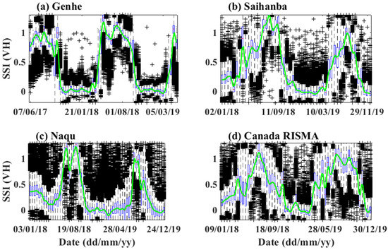
Figure 2.
Time series of boxplots of SSIS1 at VH polarization over the Genhe watershed (a), Saihanba (b), Naqu (c), and RISMA (d). On each box, the green line indicates the median, and the bottom and top edges of the box indicate the 25th and 75th percentiles, respectively. The whiskers extend to the most extreme data points not considered outliers, and the outliers are plotted individually using the ‘+’ marker symbol in black.
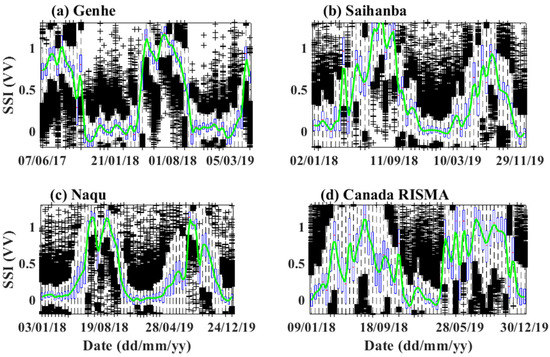
Figure 3.
Same as in Figure 2 but the boxplot of SSIS1 at VV polarization.
3.1.2. F/T Indices from Passive Microwave Observations
DFA [21,34], which is based on AMSR2 data, was chosen to detect land surface F/T states for passive microwave remote sensing data. Both the SMAP and AMSR2 F/T detection algorithms have F/T indices to identify surface F/T, while the F/T detection index of SMAP (i.e., normalized polarization ratio (NPR)) is sensitive to the change in soil liquid water content and that of AMSR2 (i.e., FTI) is sensitive to changes in soil temperature [51]. In this study, the passive microwave F/T detection index was mainly used to provide surface temperature information. DFA examines the 2-D spatial distribution of V polarization Tb of 36.5 GHz (Tb36.5 V) and the quasi-emissivity (Qe) from AMSR2 satellite data relative to signatures acquired during frozen and thawed states. These two factors can distinguish F/T by Fisher discriminant analysis. Tb36.5 V was selected because it is the most sensitive band to land surface temperature [52]. As the ratio of Tb was between any lower frequency and 36.5 V, Qe was mainly influenced by changes in the dielectric constant. Several studies [21,34,53] have used DFA to successfully monitor F/T states. To obtain the DFA over the Genhe watershed, based on the in situ 5 cm soil temperature data and AMSR2 C and Ka-band data, Fisher linear discriminant analysis was used to parameterize the DFA. The C band was chosen because of its similar wavelength to the Sentinel-1B. The FTI was computed as follows:
where FTI corresponds to the passive F/T detection index, and Tb6.925H corresponds to a Tb of 6.925 GHz at H-polarization, as H-polarization is more sensitive to soil liquid water content. The coefficients in Equation (5) are parameterized by areas with in situ 5 cm soil temperature and vary with study area and shown in Table 3. The coefficients of Genhe watershed and Saihanba are obviously different from Naqu and RISMA. Genhe watershed and Saihanba have similar location and closer coefficients. Finally, the F/T state is classified according to the following formula, where T is set to 0:

Table 3.
The coefficients in Equation (5) over four study areas.
3.2. Development of the High-Resolution F/T Detection Algorithm
The FTI and SSI have obvious F/T season characteristics, as shown in Figure 4, and can be used to detect the surface F/T state. The seasonal variation in the FTI was consistent with the seasonal changes in soil temperature. Over bare land surface, the SSI changes during the F/T transition are mainly influenced by the dielectric constant. Typically, when the soil freezing process starts, the SSI decreases rapidly due to the drastic decrease in free liquid water within the top layer of the soil surface. As the soil freezing front progresses in the deeper layers and the soil temperature decreases, the SSI decrease slows down and tends to stabilize. Similarly, during the soil thawing process, the increase in SSI is typically rapid at the beginning and slows down as the thawing process continues. Both FTI and SSI have seasonal responses to land surface F/T, thus it is potential to detect surface F/T by analyzing the relationship between the FTI and SSI. The relationship between the dielectric constant and temperature typically follows a logistic curve during the soil surface F/T process [54,55,56]. In our study area, the soil dielectric constant is mainly determined by the soil water content and its phase. A near-linear relationship between soil liquid-water content and radar backscatter has been demonstrated and implemented in high-resolution soil moisture estimation studies [37,40,57]. As SSI is linearly related to backscatter, SSI is linearly related to the dielectric constant. Zhao et al. [35] developed a high-resolution near-surface F/T detection algorithm based on the linear relationship between FTI and thermal infrared temperature with an accuracy higher than 70% over the Qinghai–Tibet Plateau region. In a study validating the performance of the DFA parameterized by Wang et al. [21] in China, Wang et al. [51] also found that the FTI was linearly correlated with surface temperature. Naeimi et al. [25] found that the behavior of backscatter concerning soil temperature followed a logistic curve in most cases based on the ASCAT data, especially in high latitude areas with sparse vegetation. Without considering the influence of vegetation on backscatter, the behavior of the SSI from the soil (noted as SSIsoil) and the FTI is expected to follow a logistic curve, similar to the relationship between the dielectric constant and soil surface temperature. The relationship between SSIsoil and FTI is expressed as follows:
where a and b are the model parameters.
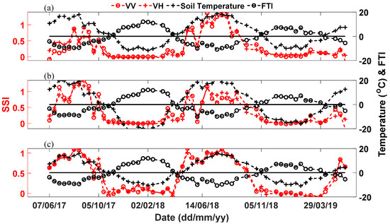
Figure 4.
An example of time series of satellite SSIS1, FTI, and in situ soil temperature for cultivated land ((a), site 11), grassland ((b), site 18), and forest ((c), site 2) over the Genhe watershed. Red line with red circle and red plus symbol are the SSI at VV and VH polarization, respectively. Black line with black circle and black plus symbol are the soil temperature and FTI, respectively.
3.2.1. AIEM Model Simulations of FTI and SSI
An analysis of the potential of combining S1 C-band data and AMSR2 data to detect land surface F/T states was carried out using simulations of Tb and backscatter. The radar backscattering coefficients and passive Tb of bare soils under frozen and unfrozen conditions were simulated using the AIEM [58], incorporated with the dielectric constant model of frozen and unfrozen soil (Zhang’s model) [55,59,60,61]. One of the factors used to determine microwave emissions from a rough surface is the dielectric constant of soil. Dobson et al. [59] developed a dielectric mixing model for thawed soil that has been widely applied in the field of microwave remote sensing. An extension of the semi-empirical dielectric constant model was developed by adding an ice item to respond to frozen conditions [55,60]. These two dielectric mixing models were used to simulate the dielectric constant of F/T soil. Mironov et al. [54] validated the Zhang’s model [55,60] with dielectric data for soils and showed that Zhang’s model could simulate the dielectric constant of frozen soil well, with root mean square errors (RMSEs) of 2.16 and 1.18 for the real and imaginary parts, respectively. AIEM was implemented to simulate the radar backscattering coefficient and Tb from the soil surface. As an improvement to the integral equation method (IEM), the AIEM reserves complementary components for the scattered fields and removes the simplifying assumption in the spectral representation of Green’s function [62]. The AIEM was used because it provides a better performance than the IEM [58]. The AIEM can better explain the surface microwave scattering and accurately simulate the ground radiometer data at AMSR-E frequencies [63,64]. The effects of frozen soil volume scattering on higher frequencies (Ku and Ka-band) rather than the C band have been observed and modeled in a few studies [65,66]. Although AIEM does not consider the volume scattering of frozen soil, it has been shown to successfully simulate surface emissions from frozen soil [34,53].
For simulations, the F/T soil dielectric constant was estimated by the dielectric mixing model. The dielectric constant estimates were set as input data for the AIEM to simulate the backscattering coefficients in VV and VH polarizations at an S1 frequency of 5.406 GHz and to calculate the passive microwave Tb at 6.925 GHz and 36.5 GHz. The input parameters for simulation of the radar backscattering coefficient and passive microwave Tb were randomly generated and are shown in Table 4. We assumed that the roughness parameters and soil texture of a fixed pixel did not change over time, and the parameter was set to a constant value.

Table 4.
Input parameters in the simulation of the radar backscattering coefficient and passive microwave Tb. RMS height indicates root mean square height. CL means correlation length.
Figure 5 shows the behavior of SSI vs. FTI based on simulation data. To highlight the relationship between the SSI and FTI in the F/T transition, the simulation data from Table 4 with soil moisture higher than 0.2 m3/m3 were selected when obvious dielectric constant changes occurred during the F/T transitions. A logistic relationship is observed between the SSI and FTI with a coefficient of determination of 0.97 from the simulation data in Figure 5.
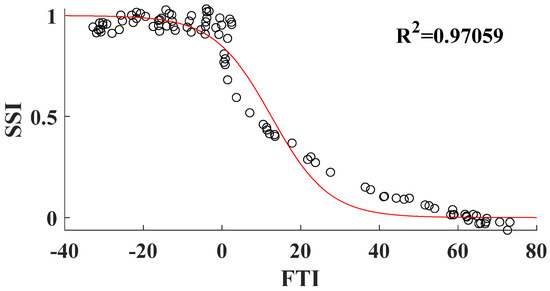
Figure 5.
Scatters between SSI and FTI from simulation data. Black circles represent the simulation data.
3.2.2. Effect of Vegetation on F/T Determination
The scatters between the satellite-based SSIS1 and FTI over cultivated land, grassland, and forest in plots Figure 6a–c follow the logistic curve with a coefficient of determination from 0.88 to 0.91. Even though the relationship between the SSIsoil and FTI in Equation (8) was established for bare land, it also applies for vegetated surfaces. The correlation coefficient is slightly lower over grassland and forest. Additionally, vegetation cover affects the surface freeze onset. The freezing onset of most vegetation-covered surfaces occurs later than that of bare land due to the insulation effect of the vegetation layer [67]. Forests and grasslands are widely distributed in the study areas. Considering the non-negligible effect of vegetation, LAI data were introduced during algorithm development. According to the water cloud model (WCM) [68,69], the backscatter from vegetation can be expressed as follows:
where E and F are the parameters of the model and is the incidence angle of radar. V1 and V2, which describe the canopy, have various descriptors in previous studies [69,70,71,72] and can be described as an exponential form of the LAI. Since SSI and backscatter are linearly correlated, the relationship between backscatter from vegetation and LAI in WCM is used to express the relationship between the SSI from vegetation (SSIveg) and the LAI. According to Equation (9), the relationship between SSIveg and LAI can be simplified as follows:
where E, F, L1, and L2 are fitting coefficients. The influence of vegetation based on Equation (10) was added to Equation (8), and the SSI can be written as follows:
where a, b, c, d, E, F, L1, and L2 are the function coefficients. Nonlinear fitting was performed pixel by pixel based on the time series of the SSIS1, FTI and LAI data. In this method, the relationships were established at the 1 km scale. The regressed coefficients were applied to the daily 1 km FTI and LAI data to estimate the new time-continuous 1 km SSI data (SSInew). Taking the three in situ sites in Figure 6 as an example, after comprehensively considering the soil information from the FTI and vegetation from the LAI, the coefficient of determination between the SSInew and SSIS1 increased to 0.92, 0.89, and 0.88 for site 12, site 3, and site 17, respectively. Figure 7 shows the relationship between SSIS1 and SSInew both considering and not considering the LAI at sites 12, 3, and 17. A small increase in the coefficient of determination can be seen when using LAI information. This improvement was mainly reflected when the value of SSI was relatively small.

Figure 6.
An example of scatters between SSIS1 and FTI from satellite data for cultivated land ((a), site 12), grassland ((b), site 3), and forest ((c), site 17) over the Genhe watershed. Black circles represent the satellite data.
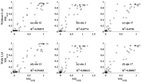
Figure 7.
Scatter plot between the SSIS1 and SSInew both considering (d–f) and not considering (a–c) the LAI for cultivated land ((a,d), site 12), grassland ((b,e), site 3), and forest ((c,f), site 17) over the Genhe watershed.
3.2.3. Pixel-Based Threshold of SSI for Detecting F/T
To detect surface F/T at the 1 km grid from the SSI, a threshold (T) needs to be determined. Previous studies basically defined T as 0.5 [23,50] or optimized it using in situ soil/air temperature data [29,30] when detecting land surface F/T with radar data. However, the feasibility of T with a fixed value or optimized value is limited by certain regions. Considering the heterogeneity of the land surface (such as land cover and terrain), a pixel-based T is defined to monitor the land surface F/T status with SSI over different areas. The T is defined as follows:
where SST_T is the threshold defined with SSI and T_min, T_max, and T_refer are the thresholds defined with ERA5-land air temperature. The ERA5-land air temperature data were used here to ensure that T is effective since the SSI_T could be very low or high and lead to low accuracy in some pixels with strong heterogeneity of land cover. To analyze the possible maximum and minimum frozen conditions, T_min and T_max are defined with time series ERA5-land daily minimum and maximum temperatures, respectively. We assume that the SSI_T should be within the range between T_min and T_max. If not, T_refer is defined with the time series ERA5-land daily 1:00 AM temperature, which corresponds to the overpass time of AMSR2. To find T_min, T_max, and T_refer, the F/T classification accuracy of SSI was validated for different threshold values (from min of SSI to max of SSI with an increment of 0.01) with ERA5-land air minimum, maximum, and 1:00 AM temperatures, respectively. The F/T status of ERA5-land air temperature is defined with a threshold of 0 °C. Then, T_min, T_max, and T_refer are found with threshold values when the accuracy is highest. However, the biases between the in situ soil temperature and ERA5-land hourly air temperature over the four study areas are −1.18 °C, −1.18 °C, −7.83 °C, and −2.1 °C over the Genhe watershed, Saihanba, Naqu, and RISMA, respectively. Considering the larger bias of ERA5-land hourly air temperature over the Naqu area, to avoid introducing more error, the SSI_T is the threshold over the Naqu area. The cold bias over the Naqu area was also reported by previous studies [73,74,75]. To define the SSI_T, we estimated the probability density distribution curve of the SSI during late autumn to early spring. The SSI_T is fitted as the SSI value that is symmetrical to the minimum values of SSI (SSI_min). The mean of the probability density distribution curve is the axis of symmetry. Figure 8 shows an example of determining SSI_T based on a histogram and the probability density distribution curve of SSInew during late autumn to early spring. Finally, the land surface F/T status was detected by SSInew based on Equations (3), (4), and (12). To compare the land surface F/T detection results with S1, Equation (12) was also applied to SSIs1 to monitor the F/T status.
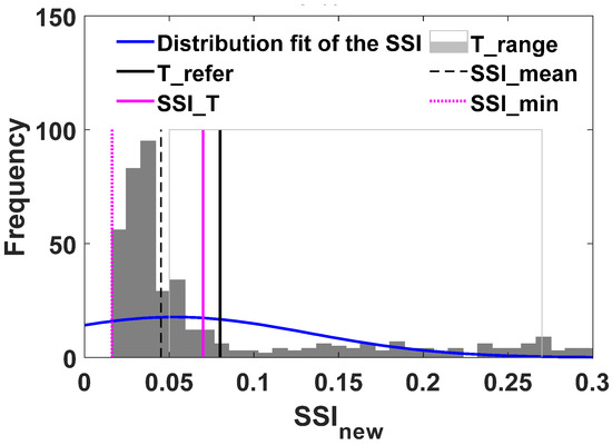
Figure 8.
An example of the SSInew histogram at site 24 during late autumn to early spring.
3.3. Evaluation Metrics
The F/T classification accuracy was evaluated using three indices [33] as follows:
where FF and TT represent the correctly classified numbers of frozen soil and thawed soil, respectively. FT and TF represent false detection flags of frozen soil and thawed soil, respectively. Equations (13)–(15) represent freeze accuracy, thaw accuracy, and overall accuracy, respectively. The in situ F/T state is defined by soil temperature data corresponding to the overpass time of AMSR2 with a threshold of 0 °C.
4. Results
4.1. F/Tnew Classification Assessment
In this section, the 5 cm depth of in situ soil temperature was used to evaluate the performance of the new F/T algorithm. Figure 9 shows the classification accuracies of F/Tnew at each site from June 2017 to May 2019 over the Genhe watershed, from August 2018 to December 2019 over Saihanba and from January 2018 to December 2019 over Naqu and RISMA. As shown in Table 5, the total accuracies for all ground sites were 93.29%, 90.79%, 88.53%, and 88.1% over the Genhe watershed, Saihanba, Naqu, and RISMA, respectively. The mean total accuracy of all study areas was 90.18%, which is higher than the required measurement accuracy (90%) of soil F/T based on the essential climate variable (ECV) observation requirements from the Global Climate Observing System (GCOS) (https://gcos.wmo.int/en/essential-climate-variables/about/requirements, accessed on 8 July 2021). Furthermore, the overall accuracies over four study areas are higher than the baseline mission requirement of 80% accuracy of SMAP [23].
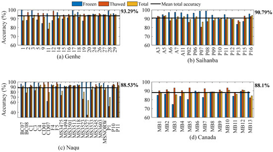
Figure 9.
The classification accuracies of F/Tnew at each site from June 2017 to May 2019 in the Genhe watershed.

Table 5.
Classification accuracy (%) statistics for F/Tnew over four study areas.
The accuracy at site 11 over the Genhe watershed area with farmland is lower than that at other sites with lower thaw accuracy. This is because the roughness of ground soil over the farmland decreased after harvest and plowing. The smoother surface caused by farming activities in the autumn would lead to a decrease in backscatter coefficients [76]. In this situation, the drop in backscatter coefficients before surface freezing may lead to false frozen flags being detected by F/Tnew. The accuracies of CD07, MS3527, and P1 over the Naqu area are significantly lower than those at other sites. Figure 10 shows the time series of the SSIS1, in situ soil moisture and ERA5-land snow depth at site MS3527 over the Naqu area. At site MS3527, SSIS1 in winter is higher (approximately 0.3) in the case of deep snow (~50 cm in December 2018) due to the effect of snow volume scattering. In Figure 10a, soil moisture increases to 0.2 m3/m3 in May and June with the thawing of the land surface and then decreases to 0.02~0.15 m3/m3 in July and August due to drought. The SSIS1 would decrease to −0.1 with decreasing soil moisture in summer. With the combined effect of deep snow in winter and drought in summer, the high values of SSIS1 in winter (~0.3) were larger than the low values of SSIS1 in summer (~−0.1), leading to false frozen flags in summer. The accuracy over RISMA with cultivated surfaces is lower than that over other study areas. Figure 11 gives the time series of the SSInew, ERA5-land temperature, in situ soil temperature and the threshold of F/T classification at site MB3 over the RISMA area. The pink dotted line is the threshold of SSInew. In Figure 11, SSInew at site MB3 in winter (~0.4) is as high as SSInew in spring, which causes false thaw flags in winter and lower frozen accuracy due to the effect of snow melting. The high SSInew in winter usually corresponded to the increase in ERA5-land air temperature when snowmelt may occur.
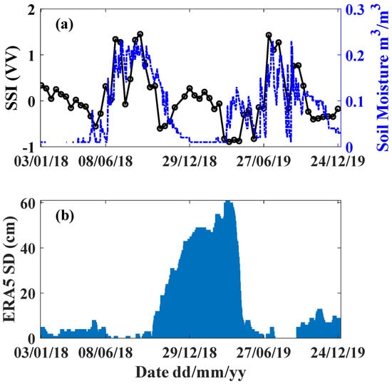
Figure 10.
Time series of the SSIS1B, in situ soil moisture and ERA5-land snow depth at site MS3527 over the Naqu area. (a) Time series of the SSIS1 (black line marked with a black circle) and in situ soil moisture (blue dashed line); (b) time series of ERA5-land snow depth.
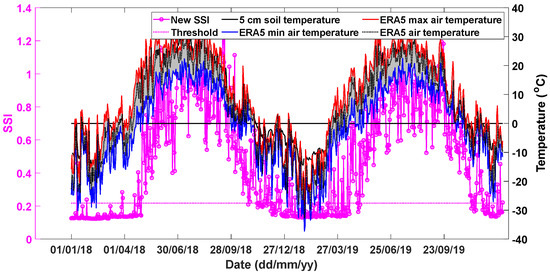
Figure 11.
Time series of the SSInew, threshold of SSInew, in situ soil and ERA5-land air temperature data at site MB3 over the RISMA area.
4.2. Comparisons of the SSIS1B and SSInew Results
In this section, to see the performance of the new algorithm (SSInew) in determining the surface F/T status, we presented an example of the spatial distribution of SSIS1B, SSInew, the retrieved F/T maps of S1B (F/TS1B), the retrieved F/T maps of SSInew (F/Tnew) and ERA5-land air temperature over the Genhe watershed. Then, time series of F/T detection results were presented over the study areas. Figure 12 provides examples of the SSIS1B ((a), (f)), the SSInew ((b), (g)), the F/TS1B ((c), (h)), the F/Tnew ((d), (i)), and the ERA5-land air temperature ((e), (j)) on 24 October 2018, 5 November 2018, respectively (i.e., the freezing period) over Genhe watershed. The spatial resolutions of SSIS1B and SSInew are 1 km, and the ERA5-land air temperature is 10 km. Although ERA5-land air temperature has a coarser spatial resolution than SSInew, it can still provide temperature distribution information for reference. Most of the SSIS1B and SSInew values over the study area decreased from approximately 0.5 to nearly 0 during this period, which indicated freezing of the land surface. The images in Figure 12b,g are the SSInew obtained from this study, which has similar spatial details to the SSIS1B (Figure 12a,f), but the value is higher than that of the SSIS1B. At the bottom of Figure 12f, the backscattering coefficients showed a distinct bright stripe, which may be caused by noise. In Figure 12g, the bright stripe was significantly improved by SSInew. The images in Figure 12c,d and Figure 12h,i can be compared with the ERA5-land air temperature images shown in Figure 12e,j. The maps of F/TS1B and F/Tnew correspond well with the ERA5-land air temperature. The land surface was mainly unfrozen on 24 October 2018 and began to freeze on 5 November 2018. In Figure 12e, the air temperature in the southwestern part of the study area is approximately 2 °C, and the corresponding F/Tnew states were mainly thawed; the temperature in the northeastern part of the study area is approximately 0 °C, and the corresponding F/Tnew states were both thawed and frozen.
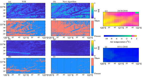
Figure 12.
Comparison examples of the spatial distribution of SSIS1B, SSInew, the F/T state retrieved from the SSIS1B, SSInew, and the ERA5-land air temperature over Genhe watershed on 24 October 2018, 5 November 2018, respectively. (SSIS1B: (a,f); SSInew: (b,g); F/TS1B: (c,h); F/Tnew: (d,i); ERA5-land air temperature: (e,j).
Figure 13, Figure 14 and Figure 15 show time series of F/Tnew, F/TS1B and air temperature over 13 days over the Genhe watershed, Saihanba and RISMA areas, 2018. During the 13 days of each area, F/Tnew provided daily F/T detection maps, while F/TS1B provided only two days of F/T detection maps. Figure 13 shows the results over the Genhe watershed from 24 October 2018 to 5 November 2018. On 24 October, the F/Tnew estimated that the study area was partly frozen, and on 25 October, it was mainly thawed, both of which correspond well with temperature. During 26–29 October, the F/Tnew maps showed increasing amounts of frozen soil as the air temperature dropped. From 30 October to 2 November, the air temperature increased, and the surface was again estimated to be thawed in the F/Tnew maps. After 3 November, the air temperature suddenly dropped, and the surface soil was estimated to be mainly frozen in the F/Tnew maps. Figure 14 shows the results over Saihanba from 10 November 2019 to 22 November 2019. During this period, the land surface was undergoing a freezing process and almost completely frozen from 15 November. Daily F/Tnew maps captured the thawing on 13–14 November and corresponded well with ERA5-land air temperature. Figure 15 shows the results over RISMA from 5 March 2019 to 17 March 2019. The surface was predominantly frozen during this time period, but a brief thaw occurred from 13 March to 15 March. The advantage of F/Tnew over F/TS1B in terms of temporal resolution is evident in capturing the land surface F/T states during the F/T transition period (i.e., spring and autumn). As mentioned in Section 3.2.3, the ERA5-land air temperature has a significant bias in the Naqu area, so the comparative analysis between daily F/Tnew and ERA5-land air temperature is not shown here.
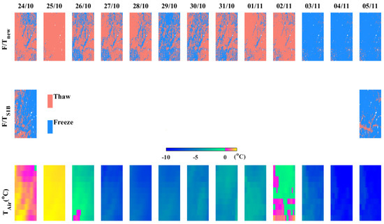
Figure 13.
Time series of F/Tnew (first line), F/TS1B (second line) and air temperature over the Genhe watershed area from 24 October 2018 to 5 November 2018.
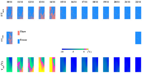
Figure 14.
Same as Figure 13 but over the Saihanba area from 10 November 2019 to 22 November 2019.
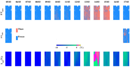
Figure 15.
Same as Figure 13 but over the RISMA area from 5 March 2019 to 17 March 2019.
5. Discussion
5.1. The Feasibility of the Method Developed in This Study
In this section, the feasibility of the method developed in this study was discussed in three stages: (1) analysis of the quality of the regression model in Equation (11) between Sentinel 1 radar, AMSR2 radiometer and GLASS LAI data; (2) exploration of the influence of the difference in the surface F/T state between the S1B and AMSR2 overpass times; and (3) discovery of the role of LAI data in the method proposed in this study.
The purpose of this paper was to estimate the land surface F/T state with a high spatial and temporal resolution and to investigate a new approach for detecting the F/T state at a high spatial resolution of 1 km by combining radar and passive remote sensing data. The high temporal and spatial surface F/T detection algorithm developed in this study is particularly useful in areas with heterogeneous land classes, soil types, and topographic distributions. Typically, for such areas, the soil F/T transitions also progress heterogeneously according to the target characteristics. In previous studies, the retrieval of high-resolution land parameters, such as the F/T state and soil moisture, was mostly based on a model established on the same scale by combining multisource remote sensing [35,38,39,57,77]. The other group of methods estimated high-resolution land parameters from coarse-scale data by introducing ancillary data to describe the spatial heterogeneity [78,79]. The method presented here is based on a nonlinear regression model between active microwave, passive microwave, and optical remote sensing data, including Sentinel 1 radar, AMSR2 radiometer, and GLASS LAI product. This study first combined these three categories of data to provide high-resolution F/T estimates both temporally and spatially. The quality of SSInew obtained by the regression model in Equation (11) was evaluated with the RMSE between SSInew and SSIS1, which is shown in Equation (16):
where m is the number of data points used for regression, is the SSInew, and is the SSIS1. Figure 16 provides the histogram and spatial distribution of RMSE over four study areas. The artificial surfaces and water bodies were masked. Except for the some mixed pixels covered with cultivated land and grassland or grassland and forest, the RMSE was lower than 0.2 over the Genhe watershed, Saihanba, and Naqu areas. Most of the RMSE in the RISMA area are below 0.25. The smaller the value of RMSE is, the smaller the difference between SSInew and SSIS1. Generally, smaller RMSE values obtained in Equation (16) correspond to a more reliable SSInew and a higher probability of accurate monitoring of land surface F/T. Figure 17 provides two examples of the relationships among SSIS1, FTI, LAI, and SSInew from the Genhe watershed, one with low RMSE (a–c) and another with high RMSE (d–f). We found that even for the high RMSE example (Figure 17d–f), the regression model could capture the soil seasonal characteristics and soil state changes. In Figure 17d, the SSIS1 increased during winter (the value of FTI was approximately 10) due to the effect of snow. Volume scattering and absorption of the microwave signal within the snow layer increases with deepening snow cover [25], which possibly leads to an increase in the SSIS1. This finding also corresponded well with Figure 10. These results demonstrate the feasibility of the regression model proposed in this paper.
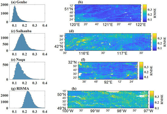
Figure 16.
The histogram and spatial distribution of the root mean square error (RMSE) between SSInew and SSIS1 of the nonlinear regression model shown in Equation (11) over the Genhe watershed (a,b), Saihanba (c,d), Naqu (e,f), and RISMA (g,h) areas.
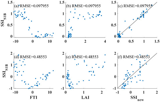
Figure 17.
Two examples of the scatter plot among the SSIS1B, FTI, LAI, and SSInew with lower RMSE (a–c) and higher RMSE (d–f) from the Genhe watershed.
The high consistency of the surface F/T state between the S1 and AMSR2 overpass times would decide the basis for algorithm development. As shown in Table 2, the overpass time of S1B over the Genhe watershed (22:00) differs the most from that of AMSR2 (1:30). To combine S1B and AMSR2 to detect the surface F/T state, an analysis was performed to determine the difference in surface F/T indicated by the in situ 5 cm soil temperature between 10:00 PM and 1:30 AM over the Genhe watershed. Figure 18 shows the comparison of in situ 5 cm soil temperature between 10:00 PM and 1:30 AM over cultivated land, grassland, and forest in the Genhe watershed. The temperatures between the two times show little difference, especially at approximately 0 °C. The consistency of surface F/T flagged at 10:00 PM and 1:30 AM was 93.72%, 98.85%, and 99.04% for cultivated land, grassland, and forest, respectively. The consistency of cultivated land was lower due to a lack of vegetation cover, which can cause a small temperature difference between 10:00 PM and 1:30 AM.
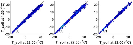
Figure 18.
Comparison of 5 cm soil temperature between S1B overpass time (22:00) and AMSR2 overpass time of the descending orbit (1:30) over cultivated (a), grassland (b), and forest (c) in the Genhe watershed.
The presented method uses the FTI and LAI to estimate the SSInew and further detects surface F/T. The FTI and SSI, as microwave-based F/T indices, are suitable for monitoring the surface F/T status. LAI data were introduced into the F/T index-based logistic model to compensate for the effect of the vegetation layer on surface F/T status determination. The vegetation layer directly influences the observations, particularly the radar signal. The vegetation layer also thermally insulates the soil beneath it, affecting the soil freezing and thawing processes. To clarify the role of LAI in detecting the surface F/T state, the F/T index-based logistic model in Equation (8) without considering the LAI was executed to estimate the SSInew_noLAI. Then, the surface F/T state was detected by the SSInew_noLAI using the same method as in the SSInew. The in situ soil temperature was used to evaluate the accuracies of F/Tnew and F/Tnew_noLAI, as shown in Figure 19. The x-axis and y-axis show the accuracies of F/Tnew and F/Tnew_noLAI, respectively. Table 6 provides the classification accuracy statistics for F/Tnew_noLAI and F/Tnew over different land cover types. Figure 20 shows the frozen days of F/Tnew and F/Tnew_noLAI from June 2017 to May 2018 over the Genhe watershed area as an example. The two indices have similar spatial distributions, but F/Tnew, which introduces high-resolution vegetation information, has more spatial details. In interlaced area of cultivated and grasslands in the southwest Genhe watershed area, frozen days of F/Tnew in Figure 20a are more than that of F/Tnew_noLAI in Figure 20b over cultivated area. In addition, in interlaced areas of grassland and forest, frozen days of F/Tnew in Figure 20a are more than that of F/Tnew_noLAI in Figure 20b over grasslands. The difference of frozen days between F/Tnew and F/Tnew_noLAI mainly occurs in the land cover which accounts for a small proportion of all land covers within passive microwave pixel. From the comparison at these four regions shown on Table 6, the overall accuracy of F/Tnew is greater than F/Tnew_noLAI over different land cover types, especially in Genhe watershed where the heterogeneity of land cover within passive microwave pixel scale is greater. The introduction of LAI data obviously improved the F/T detection accuracy in the case of heterogeneous land cover within the passive microwave pixel scale. This is because LAI can indicate high-resolution vegetation green-up date which is close to surface thawing date [80,81,82]. In summary, by introducing LAI data, the validation accuracies of the vegetation-covered surface improved, and the F/T maps had more spatial details.
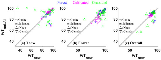
Figure 19.
A comparison of thawed (a), frozen (b) and total (c) accuracies between F/Tnew and F/Tnew_noLAI.

Table 6.
Total classification accuracy (%) statistics for F/Tnew and F/Tnew_noLAI.
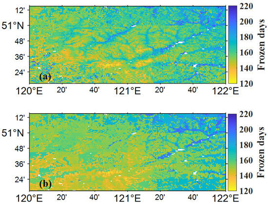
Figure 20.
The frozen days of F/Tnew (a) and F/Tnew_noLAI (b) from June 2017 to May 2018 over the Genhe watershed area as an example.
5.2. F/T Classification Accuracy Comparisons between F/TS1 and F/Tnew
Figure 21 provides comparisons of the thawed (a), frozen (b), and total (c) accuracies between F/TS1 and F/Tnew over four study areas at a 1 km resolution. Table 7 provides the classification accuracy statistics for F/TS1 and F/Tnew. The result comparisons were calculated based on all available S1 data for each study area, as shown in Table 2. The mean thaw, freezing, and total accuracies for almost all in situ sites of F/Tnew were higher than those of F/TS1 over the four study areas. The F/TS1 estimates were retrieved using only S1 radar data, and the F/Tnew estimates included the combined use of S1 and FTI data. Multifrequency passive microwave remote sensing is sensitive to both soil moisture and soil temperature and is suitable for monitoring surface F/T. Radar signals are susceptible to roughness and vegetation when monitoring surface F/T. From our results comparison, F/Tnew, which contains passive information, has higher accuracies than F/TS1. Additionally, anomalies caused by noise may exist in the S1 data (Figure 12b). SSInew could reduce abnormal phenomena by considering time series data. Therefore, F/Tnew detection had a better performance than F/TS1.
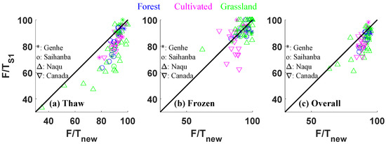
Figure 21.
Comparison of thawed (a), frozen (b), and total (c) accuracies between F/TS1 and F/Tnew at a 1 km resolution.

Table 7.
Classification accuracy (%) statistics for F/TS1 and F/Tnew.
5.3. F/T Classification Accuracy Comparisons between F/Tnew and F/TAMSR2
Figure 22 provides comparisons of the thaw (a), frozen (b), and total (c) accuracies between F/T detected from AMSR2 (F/TAMSR2) and SSInew at the site level. Table 8 provides the classification accuracy statistics for F/TAMSR2 and F/Tnew. The total accuracy of F/Tnew was higher than that of F/TAMSR2, while F/TAMSR2 had a higher thaw accuracy. The theoretical soil penetration depth of the C band is 1–5 cm [83]. Unlike the F/T detection algorithm of AMSR2, which could reflect the 5 cm depth F/T state because it was parameterized by the 5 cm depth soil temperature, the F/Tnew detected F/T using the C band, which cannot reflect the soil F/T at the 5 cm depth. Even though the soil at the 5 cm depth was thawed, it could not be detected by F/Tnew with the C band. Thus, F/Tnew detected more frozen soil than F/TAMSR2. Figure 23 shows the frozen days calculated from the F/Tnew (a) at 1 km and F/TAMSR2 (b) at 25 km from June 2017 to May 2018 over the Genhe watershed area as an example. The white color in Figure 23a indicates artificial surfaces and water bodies that were masked. Additionally, the spatial patterns of frozen days calculated from the F/Tnew and F/TAMSR2 data were similar over the study area, with the spatial trend of fewer frozen days in the southwestern part and more in the northeastern part of the study area. The frozen days calculated from the F/Tnew obviously have more details than that of AMSR2.
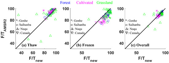
Figure 22.
Comparisons of thawed (a), frozen (b), and total (c) accuracies between F/TAMSR2 and F/Tnew at the site level.

Table 8.
Classification accuracy (%) statistics for F/TAMSR2 and F/Tnew.
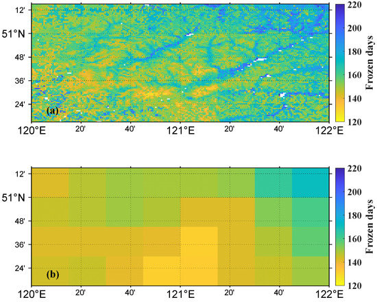
Figure 23.
Frozen days calculated from the F/Tnew (a) at 1 km and F/TAMSR2 (b) at 25 km from June 2017 to May 2018.
6. Conclusions
This paper investigated a new approach for detecting daily land surface F/T at 1 km with AMSR2, S1 and LAI data over the Genhe watershed, the Saihanba and Naqu area located in China and the RISMA network located in Canada, respectively. The proposed approach is derived based on a logistic relationship between the SSIS1 derived from Sentinel-1 SAR data and AMSR2 FTI. The logistic relation was confirmed by AIEM simulations and observational data. Since vegetation affects microwave signals and the freezing time of the land surface, LAI data were introduced to express the influence of vegetation and provide spatial patterns at the kilometer scale for F/T status determination. The daily F/T state at 1 km could be estimated from the SSInew obtained from FTI and LAI data. The in situ 5 cm depth soil temperature data from four soil temperature measurement networks were used to evaluate the classification accuracies of F/Tnew. The mean total accuracies obtained from in situ sites are 93.29%, 90.79%, 88.53%, and 88.1% over the Genhe watershed, Saihanba, Naqu and RISMA, respectively. By introducing LAI data, the classification accuracies of F/Tnew over the vegetation-covered surface maximum increased by 7.6%. The results comparison between F/Tnew and F/TS1 at 1 km showed that this method could reduce some S1 data anomalies and obtain higher accuracies. Additionally, the accuracy comparison results between F/Tnew at 1 km and F/TAMSR2 at 25 km showed that the high-resolution results could more accurately reflect the land surface state. In this study, daily 1 km land surface F/T could be detected by combining with Sentinel-1 SAR, AMSR2, and LAI data. The accuracy increased by 5.17% and 0.85%, reaching 90% and 90.18% when compared with the stand-alone S1 F/T results at 0.01° and the AMSR2 F/T results at 0.25° resolution. Despite this method may be affected by the change in roughness over cultivated areas caused by agricultural activity, leading to false detection flags for thaw surfaces. The overall accuracy over cultivated areas was still above 90%. This indicated that combined SAR and passive microwave remote sensing can monitor relatively high spatial resolution surface F/T at 1 km with high accurately than through passive satellite sensors. The accuracies have improved over vegetation-covered surfaces by considering the effect of vegetation.
The combination of S1 and AMSR2 has the potential to detect land surface F/T states with high spatial and temporal resolutions over a large scale, even at the global scale. In future work, we will apply a temperature-based filter to remove false detections during winter caused by the snow effect. In addition, the new approach developed in this work is established based on time series data for each pixel, and the algorithm coefficients obtained from the available Sentinel-1 data could be used to estimate the SSInew during periods before Sentinel-1 was launched. Thus, the daily land surface F/T state at 1 km before the launch of Sentinel-1 could be estimated. It is expected to derive a long series of daily land surface F/T states at a spatial resolution of 1 km since 2002.
Author Contributions
Data curation, C.Z., Z.X., H.L., J.Y. and H.C.; Funding acquisition, L.J.; Investigation, J.W. and K.R.; Methodology, J.W. and L.J.; Supervision, L.J.; Validation, J.W.; Writing—Original draft, J.W., L.J. and K.R. All authors have read and agreed to the published version of the manuscript.
Funding
This research was funded by the National Key Research and Development Program of China, grant number 2021YFB3900104; the Second Tibetan Plateau Scientific Expedition and Research Program, grant number 2019QZKK0206; and the National Natural Science Foundation of China, grant number 42090014, and 42171317.
Acknowledgments
We would also like to thank the Japan Aerospace Exploration Agency for providing the AMSR2 L3 data and the European Space Agency for providing the Sentinel-1 data.
Conflicts of Interest
The authors declare no conflict of interest.
References
- Zhang, T.J.; Armstrong, R.L.; Smith, J. Investigation of the near-surface soil freeze-thaw cycle in the contiguous United States: Algorithm development and validation. J. Geophys. Res. Atmos. 2003, 108, 8860. [Google Scholar] [CrossRef] [Green Version]
- Kimball, J.S.; Mcdonald, K.C.; Frolking, S.E.; Running, S.W. Radar remote sensing of the spring thaw transition across a boreal landscape. Remote Sens. Environ. 2004, 89, 163–175. [Google Scholar] [CrossRef]
- McDonald, K.C.; Kimball, J.S. Estimation of Surface Freeze–Thaw States Using Microwave Sensors. In Encyclopedia of Hydrological Sciences; Anderson, M.G., Ed.; John Wiley & Sons, Ltd.: Hoboken, NJ, USA, 2005; pp. 783–797. [Google Scholar]
- Zhang, X.; Zhang, H.; Wang, C.; Tang, Y.; Zhang, B.; Wu, F.; Wang, J.; Zhang, Z. Time-Series InSAR Monitoring of Permafrost Freeze-Thaw Seasonal Displacement over Qinghai–Tibetan Plateau Using Sentinel-1 Data. Remote Sens. 2019, 11, 1000. [Google Scholar] [CrossRef] [Green Version]
- Lu, P.; Han, J.; Hao, T.; Li, R.; Qiao, G. Seasonal Deformation of Permafrost in Wudaoliang Basin in Qinghai-Tibet Plateau Revealed by StaMPS-InSAR. Mar. Geod. 2020, 43, 248–268. [Google Scholar] [CrossRef]
- Wang, J.; Wang, C.; Zhang, H.; Tang, Y.; Zhang, X.; Zhang, Z. Small-Baseline Approach for Monitoring the Freezing and Thawing Deformation of Permafrost on the Beiluhe Basin, Tibetan Plateau Using TerraSAR-X and Sentinel-1 Data. Sensors 2020, 20, 4464. [Google Scholar] [CrossRef] [PubMed]
- Gabrielle, W. Climate Change 2007: A world melting from the top down. Nature 2007, 446, 718–721. [Google Scholar] [CrossRef]
- Schuur, E.A.G.; Abbott, B. High risk of permafrost thaw. Nature 2011, 480, 32–33. [Google Scholar] [CrossRef]
- Christensen, T.R. It’s a gas. Nat. Geosci. 2016, 9, 647–648. [Google Scholar] [CrossRef]
- Wang, J.Y.; Song, C.C.; Hou, A.X.; Xi, F.M. Methane Emission Potential from Freshwater Marsh Soils of Northeast China: Response to Simulated Freezing-Thawing Cycles. Wetlands 2017, 37, 437–445. [Google Scholar] [CrossRef]
- Swindles, G.T.; Morris, P.J.; Mullan, D.; Watson, E.J.; Turner, T.E.; Roland, T.P.; Amesbury, M.J.; Kokfelt, U.; Schoning, K.; Pratte, S.; et al. The long-term fate of permafrost peatlands under rapid climate warming. Sci. Rep. 2015, 5, 17951. [Google Scholar] [CrossRef] [Green Version]
- Shugar, D.H.; Jacquemart, M.; Shean, D.; Bhushan, S.; Upadhyay, K.; Sattar, A.; Schwanghart, W.; McBride, S.; de Vries, M.V.; Mergili, M.; et al. A massive rock and ice avalanche caused the 2021 disaster at Chamoli, Indian Himalaya. Science 2021, 373, 300–306. [Google Scholar] [CrossRef] [PubMed]
- Zhang, Y.; Touzi, R.; Feng, W.; Hong, G.; Lantz, T.C.; Kokelj, S.V. Landscape-scale variations in near-surface soil temperature and active-layer thickness: Implications for high-resolution permafrost mapping. Permafr. Periglac. Process. 2021, 32, 627–640. [Google Scholar] [CrossRef]
- Black, R.F. Features Indicative of Permafrost. Annu. Rev. Earth Planet. Sci. 1976, 4, 75–94. [Google Scholar] [CrossRef]
- Davitt, A.; Schumann, G.; Forgotson, C.; McDonald, K.C. The Utility of SMAP Soil Moisture and Freeze-Thaw Datasets as Precursors to Spring-Melt Flood Conditions: A Case Study in the Red River of the North Basin. IEEE J. Sel. Top. Appl. Earth Obs. Remote Sens. 2019, 12, 2848–2861. [Google Scholar] [CrossRef]
- Guo, B.; Zhou, Y.; Zhu, J.; Liu, W.; Wang, F.; Wang, L.; Jiang, L. An estimation method of soil freeze-thaw erosion in the Qinghai–Tibet Plateau. Nat. Hazards 2015, 78, 1843–1857. [Google Scholar] [CrossRef]
- Zuerndorfer, B.; England, A.W. Radiobrightness decision criteria for freeze/thaw boundaries. IEEE Trans. Geosci. Remote Sens. 1992, 30, 89–102. [Google Scholar] [CrossRef]
- Rignot, E.; Way, J.B. Monitoring freeze—thaw cycles along North—South Alaskan transects using ERS-1 SAR. Remote Sens. Environ. 1994, 49, 131–137. [Google Scholar] [CrossRef] [Green Version]
- Watanabe, K.; Wake, T. Measurement of unfrozen water content and relative permittivity of frozen unsaturated soil using NMR and TDR. Cold Reg. Sci. Technol. 2009, 59, 34–41. [Google Scholar] [CrossRef]
- Kim, Y.; Kimball, J.S.; Glassy, J.; Du, J.Y. An Extended Global Earth System Data Record on Daily Landscape Freeze-Thaw Status Determined from Satellite Passive Microwave Remote Sensing. Earth Syst. Sci. Data 2017, 9, 133–147. [Google Scholar] [CrossRef] [Green Version]
- Wang, P.K.; Zhao, T.J.; Shi, J.C.; Hu, T.X.; Roy, A.; Qiu, Y.B.; Lu, H. Parameterization of the freeze/thaw discriminant function algorithm using dense in-situ observation network data. Int. J. Digit. Earth 2018, 12, 980–994. [Google Scholar] [CrossRef]
- Rautiainen, K.; Parkkinen, T.; Lemmetyinen, J.; Schwank, M.; Wiesmann, A.; Ikonen, J.; Derksen, C.; Davydov, S.; Davydova, A.; Boike, J. SMOS prototype algorithm for detecting autumn soil freezing. Remote Sens. Environ. 2016, 180, 346–360. [Google Scholar] [CrossRef]
- Derksen, C.; Xu, X.L.; Dunbar, R.S.; Colliander, A.; Kim, Y.; Kimball, J.S.; Black, T.A.; Euskirchen, E.; Langlois, A.; Loranty, M.M. Retrieving landscape freeze/thaw state from Soil Moisture Active Passive (SMAP) radar and radiometer measurements. Remote Sens. Environ. 2017, 194, 48–62. [Google Scholar] [CrossRef]
- Prince, M.; Roy, A.; Brucker, L.; Royer, A.; Kim, Y.; Zhao, T.J. Northern Hemisphere surface freeze-thaw product from Aquarius L-band radiometers. Earth Syst. Sci. Data 2018, 10, 2055–2067. [Google Scholar] [CrossRef] [Green Version]
- Naeimi, V.; Paulik, C.; Bartsch, A.; Wagner, W.; Kidd, R.; Park, S.E.; Elger, K.; Boike, J. ASCAT Surface State Flag (SSF): Extracting Information on Surface Freeze/Thaw Conditions From Backscatter Data Using an Empirical Threshold-Analysis Algorithm. IEEE Trans. Geosci. Remote Sens. 2012, 50, 2566–2582. [Google Scholar] [CrossRef]
- Park, S.-E. Variations of Microwave Scattering Properties by Seasonal Freeze/Thaw Transition in the Permafrost Active Layer Observed by ALOS PALSAR Polarimetric Data. Remote Sens. 2015, 7, 17135–17148. [Google Scholar] [CrossRef] [Green Version]
- Muhuri, A.; Manickam, S.; Bhattacharya, A. Snow Cover Mapping Using Polarization Fraction Variation with Temporal RADARSAT-2 C-Band Full-Polarimetric SAR Data Over the Indian Himalayas. IEEE J. Sel. Top. Appl. Earth Obs. Remote Sens. 2018, 11, 2192–2209. [Google Scholar] [CrossRef]
- Azarderakhsh, M.; McDonald, K.; Norouzi, H.; Barros, A.; Arunvavikul, P.; Blake, R. Using Sentinel-L Sar Measurements to Detect High Resolution Freeze and Thaw States in Alaska. In Proceedings of the IGARSS 2018–2018 IEEE International Geoscience and Remote Sensing Symposium, Valencia, Spain, 22–27 July 2018; pp. 2398–2399. [Google Scholar]
- Baghdadi, N.; Bazzi, H.; El Hajj, M.; Zribi, M. Detection of Frozen Soil Using Sentinel-1 SAR Data. Remote Sens. 2018, 10, 15. [Google Scholar] [CrossRef] [Green Version]
- Fayad, I.; Baghdadi, N.; Bazzi, H.; Zribi, M. Near Real-Time Freeze Detection over Agricultural Plots Using Sentinel-1 Data. Remote Sens. 2020, 12, 1976. [Google Scholar] [CrossRef]
- Cohen, J.; Rautiainen, K.; Ikonen, J.; Lemmetyinen, J.; Smolander, T.; Vehvilêinen, J.; Pulliainen, J. A Modeling-Based Approach for Soil Frost Detection in the Northern Boreal Forest Region with C-Band SAR. IEEE Trans. Geosci. Remote Sens. 2019, 57, 1069–1083. [Google Scholar] [CrossRef]
- Cohen, J.; Rautiainen, K.; Lemmetyinen, J.; Smolander, T.; Vehvilainen, J.; Pulliainen, J. Sentinel-1 based soil freeze/thaw estimation in boreal forest environments. Remote Sens. Environ. 2021, 254, 112267. [Google Scholar] [CrossRef]
- Kou, X.K.; Jiang, L.M.; Yan, S.; Zhao, T.J.; Lu, H.; Cui, H.Z. Detection of land surface freeze-thaw status on the Tibetan Plateau using passive microwave and thermal infrared remote sensing data. Remote Sens. Environ. 2017, 199, 291–301. [Google Scholar] [CrossRef]
- Zhao, T.J.; Zhang, L.X.; Jiang, L.M.; Zhao, S.J.; Chai, L.N.; Jin, R. A new soil freeze/thaw discriminant algorithm using AMSR-E passive microwave imagery. Hydrol. Process. 2011, 25, 1704–1716. [Google Scholar] [CrossRef]
- Zhao, T.; Shi, J.; Hu, T.; Zhao, L.; Zou, D.; Wang, T.; Ji, D.; Li, R.; Wang, P. Estimation of High-resolution Near-surface Freeze/thaw State by the Integration of Microwave and Thermal Infrared Remote Sensing Data on the Tibetan Plateau. Earth Space Sci. 2017, 4, 472–484. [Google Scholar] [CrossRef]
- Zhong, W.; Yuan, Q.; Liu, T.; Yue, L. Freeze/thaw onset detection combining SMAP and ASCAT data over Alaska: A machine learning approach. J. Hydrol. 2022, 605, 127354. [Google Scholar] [CrossRef]
- Das, N.N.; Entekhabi, D.; Njoku, E.G. An Algorithm for Merging SMAP Radiometer and Radar Data for High-Resolution Soil-Moisture Retrieval. IEEE Trans. Geosci. Remote Sens. 2011, 49, 1504–1512. [Google Scholar] [CrossRef]
- Das, N.N.; Entekhabi, D.; Kim, S.; Jagdhuber, T.; Dunbar, S.; Yueh, S.; Colliander, A. High-Resolution Enhanced Product based on SMAP Active-Passive Approach using Sentinel 1 Data and its Applications. In Proceedings of the 2017 IEEE International Geoscience and Remote Sensing Symposium, Fort Worth, TX, USA, 23–28 July 2017; IEEE: New York, NY, USA, 2017; pp. 2493–2494. [Google Scholar]
- Das, N.N.; Entekhabi, D.; Dunbar, R.S.; Chaubell, M.J.; Colliander, A.; Yueh, S.; Jagdhuber, T.; Chen, F.; Crow, W.; O’Neill, P.E.; et al. The SMAP and Copernicus Sentinel 1A/B microwave active-passive high resolution surface soil moisture product. Remote Sens. Environ. 2019, 233, 17. [Google Scholar] [CrossRef]
- Piles, M.; Entekhabi, D.; Camps, A. A Change Detection Algorithm for Retrieving High-Resolution Soil Moisture From SMAP Radar and Radiometer Observations. IEEE Trans. Geosci. Remote Sens. 2009, 47, 4125–4131. [Google Scholar] [CrossRef]
- Jiang, L.; Wang, J.; Cui, H.; Wang, G.; Zhao, T.; Zhao, S.; Chai, L.; Liu, X.; Yang, J. In situ soil moisture and temperature network in genhe watershed and saihanba area in China. Data Brief 2020, 31, 105693. [Google Scholar] [CrossRef]
- Cui, H.Z.; Jiang, L.M.; Du, J.Y.; Zhao, S.J.; Wang, G.X.; Lu, Z.; Wang, J. Evaluation and analysis of AMSR-2, SMOS, and SMAP soil moisture products in the Genhe area of China. J. Geophys. Res. Atmos. 2017, 122, 8650–8666. [Google Scholar] [CrossRef]
- Yang, K.; Qin, J.; Zhao, L.; Chen, Y.Y.; Tang, W.J.; Han, M.L.; Lazhu; Chen, Z.Q.; Lv, N.; Ding, B.H. A Multi-Scale Soil Moisture and Freeze-Thaw Monitoring Network on the Third Pole. Bull. Am. Meteorol. Soc. 2013, 94, 1907–1916. [Google Scholar] [CrossRef]
- Ojo, E.R.; Bullock, P.; L’Heureux, J.; Powers, J.; McNairn, H.; Pacheco, A. Calibration and Evaluation of a Frequency Domain Reflectometry Sensor for Real-Time Soil Moisture Monitoring. Vadose Zone J. 2015, 14, vzj2014.08.0114. [Google Scholar] [CrossRef]
- Chen, J.; Chen, J.; Liao, A.P.; Cao, X.; Chen, L.J.; Chen, X.H.; He, C.Y.; Han, G.; Peng, S.; Lu, M.; et al. Global land cover mapping at 30 m resolution: A POK-based operational approach. Isprs J. Photogramm. Remote Sens. 2015, 103, 7–27. [Google Scholar] [CrossRef] [Green Version]
- Baghdadi, N.; Bernier, M.; Gauthier, R.; Neeson, I. Evaluation of C-band SAR data for wetlands mapping. Int. J. Remote Sens. 2001, 22, 71–88. [Google Scholar] [CrossRef]
- Konstantinos, T.; Suman, S.; Dimitra, K. Incidence angle normalization of Wide Swath SAR data for oceanographic applications. Open Geosci. 2016, 8, 450–464. [Google Scholar] [CrossRef] [Green Version]
- Xiao, Z.; Liang, S.; Wang, J.; Chen, P.; Yin, X.; Zhang, L.; Song, J. Use of General Regression Neural Networks for Generating the GLASS Leaf Area Index Product From Time-Series MODIS Surface Reflectance. IEEE Trans. Geosci. Remote Sens. 2014, 52, 209–223. [Google Scholar] [CrossRef]
- Xiao, Z.Q.; Liang, S.L.; Wang, J.D.; Xiang, Y.; Zhao, X.; Song, J.L. Long-Time-Series Global Land Surface Satellite Leaf Area Index Product Derived From MODIS and AVHRR Surface Reflectance. IEEE Trans. Geosci. Remote Sens. 2016, 54, 5301–5318. [Google Scholar] [CrossRef]
- Rodionova, N.V. Identification of Frozen/Thawed Soils in the Areas of Anadyr (Chukotka) and Belaya Gora (Sakha) from the Sentinel 1 Radar Data. Izv. Atmos. Ocean. Phys. 2019, 55, 1314–1321. [Google Scholar] [CrossRef]
- Wang, J.; Jiang, L.M.; Cui, H.Z.; Wang, G.X.; Yang, J.W.; Liu, X.J.; Su, X. Evaluation and analysis of SMAP, AMSR2 and MEaSUREs freeze/thaw products in China. Remote Sens. Environ. 2020, 242, 111734. [Google Scholar] [CrossRef]
- Mcfarland, M.J.; Miller, R.L.; Neale, C.M.U. Land surface temperature derived from the SSM/I passive microwave brightness temperatures. IEEE Trans. Geosci. Remote Sens. 1990, 28, 839–845. [Google Scholar] [CrossRef]
- Kou, X.K.; Jiang, L.M.; Yan, S.; Wang, J.; Gao, L.Y. Research on the Improvement of Passive Microwave Freezing and Thawing Discriminant Algorithms for Complicated Surface Conditions. In Proceedings of the IEEE International Symposium on Geoscience and Remote Sensing, Valencia, Spain, 22–27 July 2018; pp. 7161–7164. [Google Scholar]
- Mironov, V.L.; Kosolapova, L.G.; Lukin, Y.I.; Karavaysky, A.Y.; Molostov, I.P. Temperature- and texture-dependent dielectric model for frozen and thawed mineral soils at a frequency of 1.4GHz. Remote Sens. Environ. 2017, 200, 240–249. [Google Scholar] [CrossRef]
- Zhang, L.X.; Shi, J.C.; Zhang, Z.J.; Zhao, K.G. The estimation of dielectric constant of frozen soil-water mixture at microwave bands. In Proceedings of the IEEE International Symposium on Geoscience and Remote Sensing, Toulouse, France, 21–25 July 2003; pp. 2903–2905. [Google Scholar]
- Hallikainen, M.; Ulaby, F.T.; Dobson, M.; El-Rayes, M. Dielectric measurements of soils in the 3- to 37-GHz band between-50 °C and 23 °C. In Proceeding of International Geoscience and Remote Sensing Symposium, (IGARSS’84), Strasbourg, France, 27–30 August 1984; pp. 163–168. [Google Scholar]
- He, L.; Hong, Y.; Wu, X.L.; Ye, N.; Walker, J.P.; Chen, X.N. Investigation of SMAP Active-Passive Downscaling Algorithms Using Combined Sentinel-1 SAR and SMAP Radiometer Data. IEEE Trans. Geosci. Remote Sens. 2018, 56, 4906–4918. [Google Scholar] [CrossRef]
- Chen, K.S.; Tzong-Dar, W.; Leung, T.; Qin, L.; Jiancheng, S.; Fung, A.K. Emission of rough surfaces calculated by the integral equation method with comparison to three-dimensional moment method simulations. IEEE Trans. Geosci. Remote Sens. 2003, 41, 90–101. [Google Scholar] [CrossRef]
- Dobson, M.C.; Ulaby, F.T.; Hallikainen, M.T.; El-rayes, M.A. Microwave Dielectric Behavior of Wet Soil-Part II: Dielectric Mixing Models. IEEE Trans. Geosci. Remote Sens. 1985, GE-23, 35–46. [Google Scholar] [CrossRef]
- Zhang, L.; Zhao, T.; Jiang, L.; Zhao, S. Estimate of Phase Transition Water Content in Freeze–Thaw Process Using Microwave Radiometer. IEEE Trans. Geosci. Remote Sens. 2010, 48, 4248–4255. [Google Scholar] [CrossRef]
- Wu, S.; Zhao, T.; Pan, J.; Xue, H.; Zhao, L.; Shi, J. Improvement in Modeling Soil Dielectric Properties during Freeze-Thaw Transitions. IEEE Geosci. Remote Sens. Lett. 2022, 19, 2001005. [Google Scholar] [CrossRef]
- Fung, A.K.; Li, Z.; Chen, K.S. Backscattering from a randomly rough dielectric surface. IEEE Trans. Geosci. Remote Sens. 1992, 30, 356–369. [Google Scholar] [CrossRef]
- Shi, J.; Jiang, L.; Zhang, L.; Chen, K.-S.; Wigneron, J.; Chanzy, A. A parameterized multifrequency-polarization surface emission model. IEEE Trans. Geosci. Remote Sens. 2005, 43, 2831–2841. [Google Scholar] [CrossRef]
- Zhang, L.; Zhao, K.; Zhu, Y.; Qin, B. Simulated radiation characteristics of frozen soil surface at typical microwave bands. In Proceedings of the IGARSS 2004, 2004 IEEE International Geoscience and Remote Sensing Symposium, Anchorage, Alaska, 20–24 September 2004; Volume 4316, pp. 4310–4313. [Google Scholar]
- England, A.W.; Galantowicz, J.F.; Zuerndorfer, B.W. A volume scattering explanation for the negative spectral gradient of frozen soil. In Proceedings of the IGARSS’91 Remote Sensing: Global Monitoring for Earth Management, Espoo, Finland, 3–6 June 1991; pp. 1175–1177. [Google Scholar]
- Hao, Z.; Zhao, S.; Zhang, L.; Jiang, L.; Xiao, L. Comparison of microwave emission model for frozen soil and field observation. In Proceedings of the 2011 IEEE International Geoscience and Remote Sensing Symposium, Vancouver, BC, Canada, 24–29 July 2011; pp. 3097–3100. [Google Scholar]
- Wang, J.; Jiang, L.; Kou, X.; Cui, H.; Yang, J. Downscaling method for near-surface freeze/thaw state monitoring in Genhe area of China. J. Remote Sens. 2019, 26, 1209–1222. [Google Scholar] [CrossRef]
- Attema, E.P.W.; Ulaby, F.T. Vegetation modeled as a water cloud. Radio Sci. 1978, 13, 357–364. [Google Scholar] [CrossRef]
- Prévot, L.; Champion, I.; Guyot, G. Estimating surface soil moisture and leaf area index of a wheat canopy using a dual-frequency (C and X bands) scatterometer. Remote Sens. Environ. 1993, 46, 331–339. [Google Scholar] [CrossRef]
- Ulaby, F.T.; Allen, C.T.; Eger, G.; Kanemasu, E. Relating the microwave backscattering coefficient to leaf area index. Remote Sens. Environ. 1984, 14, 113–133. [Google Scholar] [CrossRef]
- Lievens, H.; Verhoest, N.E.C. On the Retrieval of Soil Moisture in Wheat Fields From L-Band SAR Based on Water Cloud Modeling, the IEM, and Effective Roughness Parameters. IEEE Geosci. Remote Sens. Lett. 2011, 8, 740–744. [Google Scholar] [CrossRef]
- Hosseini, M.; McNairn, H.; Merzouki, A.; Pacheco, A. Estimation of Leaf Area Index (LAI) in corn and soybeans using multi-polarization C- and L-band radar data. Remote Sens. Environ. 2015, 170, 77–89. [Google Scholar] [CrossRef]
- Cao, B.; Gruber, S.; Zheng, D.; Li, X. The ERA5-Land soil temperature bias in permafrost regions. Cryosphere 2020, 14, 2581–2595. [Google Scholar] [CrossRef]
- Hu, G.; Zhao, L.; Li, R.; Wu, X.; Wu, T.; Xie, C.; Zhu, X.; Su, Y. Variations in soil temperature from 1980 to 2015 in permafrost regions on the Qinghai-Tibetan Plateau based on observed and reanalysis products. Geoderma 2019, 337, 893–905. [Google Scholar] [CrossRef]
- Yang, K.; Zhang, J. Evaluation of reanalysis datasets against observational soil temperature data over China. Clim. Dyn. 2018, 50, 317–337. [Google Scholar] [CrossRef]
- Zribi, M.; Dechambre, M. A new empirical model to retrieve soil moisture and roughness from C-band radar data. Remote Sens. Environ. 2003, 84, 42–52. [Google Scholar] [CrossRef]
- Das, N.N.; Entekhabi, D.; Kim, S.; Jagdhuber, T.; Dunbar, S.; Yueh, S.; O’Neill, P.E.; Colliander, A.; Walker, J.; Jackson, T.J.; et al. High resolution soil moisture product based on smap active-passive approach using copernicus sentinel 1 data. In Proceedings of the Igarss 2018-2018 IEEE International Geoscience and Remote Sensing Symposium, Valencia, Spain, 22–27 July 2018; IEEE: New York, NY, USA, 2018; pp. 3768–3770. [Google Scholar]
- Alemohammad, S.H.; Kolassa, J.; Prigent, C.; Aires, F.; Gentine, P. Global downscaling of remotely sensed soil moisture using neural networks. Hydrol. Earth Syst. Sci. 2018, 22, 5341–5356. [Google Scholar] [CrossRef] [Green Version]
- Zhang, X.D.; Zhou, J.; Gottsche, F.M.; Zhan, W.F.; Liu, S.M.; Cao, R.Y. A Method Based on Temporal Component Decomposition for Estimating 1-km All-Weather Land Surface Temperature by Merging Satellite Thermal Infrared and Passive Microwave Observations. IEEE Trans. Geosci. Remote Sens. 2019, 57, 4670–4691. [Google Scholar] [CrossRef]
- Che, D.; Chen, B.; Zhang, H.; Fang, S.; Xu, G.; Lin, X.; Wang, Y. A New Equation for Deriving Vegetation Phenophase from Time Series of Leaf Area Index (LAI) Data. Remote Sens. 2014, 6, 5650–5670. [Google Scholar] [CrossRef] [Green Version]
- Jiang, H.; Zhang, W.; Yi, Y.; Yang, K.; Li, G.; Wang, G. The impacts of soil freeze/thaw dynamics on soil water transfer and spring phenology in the Tibetan Plateau. Arct. Antarct. Alp. Res. 2018, 50, e1439155. [Google Scholar] [CrossRef] [Green Version]
- Wang, X.; Jin, R.; Du, P.; Hao, D. Trend of surface freeze-thaw cycles and vegetation green-up date and their response to climate change on the Qinghai-Tibet Plateau. J. Remote Sens. 2018, 22, 508–520. [Google Scholar] [CrossRef]
- Ulaby, F.; Moore, R.; Fung, A. Microwave Remote Sensing: Active and Passive. Volume 2-Radar Remote Sensing and Surface Scattering and Emission Theory; Addison-Wesley: Norwood, MA, USA, 1982. [Google Scholar]
Publisher’s Note: MDPI stays neutral with regard to jurisdictional claims in published maps and institutional affiliations. |
© 2022 by the authors. Licensee MDPI, Basel, Switzerland. This article is an open access article distributed under the terms and conditions of the Creative Commons Attribution (CC BY) license (https://creativecommons.org/licenses/by/4.0/).