Abstract
The increase in remote sensing satellite imagery with high spatial and temporal resolutions has enabled the development of a wide variety of applications for Earth observation and monitoring. At the same time, it requires new techniques that are able to manage the amount of data stored and transmitted to the ground. Advanced techniques for on-board data processing answer this problem, offering the possibility to select only the data of interest for a specific application or to extract specific information from data. However, the computational resources that exist on-board are limited compared to the ground segment availability. Alternatively, in applications such as change detection, only images containing changes are useful and worth being stored and sent to the ground. In this paper, we propose a change detection scheme that could be run on-board. It relies on a feature-based representation of the acquired images which is obtained by means of an auto-associative neural network (AANN). Once the AANN is trained, the dissimilarity between two images is evaluated in terms of the extracted features. This information can be subsequently turned into a change detection result. This study, which presents one of the first techniques for on-board change detection, yielded encouraging results on a set of Sentinel-2 images, even in light of comparison with a benchmark technique.
1. Introduction
Remote sensing satellites acquire useful data for environmental monitoring, such as land cover and land use surveys, urban studies and hazard management, collecting images that provide a global and rapid response of the involved areas [1,2,3]. In the traditional processing chain, acquired images are downlinked to the ground for analysis and distribution operations. However, the increasing size of data produced by the Earth observation satellites requires innovative processing techniques. For this reason, intelligent on-board data processing and data-reduction procedures are becoming essential in current and planned missions [4]. In fact, the high-resolution instruments in use produce huge sensor data volumes, which demand high on-board data storage capacity and communication resources, i.e., bandwidth, for data downlinking to end users on the ground. In order to face both the memory and bandwidth availabilities, many future satellite missions are working with the purpose of moving data processing from the ground segment to the space segment through on-board processing operations. In this context, a particular focus regards data management in small satellites. Small satellites have become increasingly popular due to their small size, low power consumption, short development cycle and low cost. However, they are subject to limited on-board transmitting power and limited communication band choices, as well as restricted storage space, so a new processing flow is required rather than the traditional one [5]. Therefore, having the possibility to directly deliver the concerned higher-level information contained in the remote sensing images becomes crucial; this is indeed usually many orders of magnitude smaller than the remote sensing data themselves. Moreover, the processed results will greatly improve the downlink data transmission efficiency, allowing for reduction in the transmission bandwidth and enhancing the transmission rate. Additionally, by selecting only the useful information, the on-board platform memory cost can be reduced [6,7].
On-board processing requires several characteristics, such as flexibility, robustness, low computation burden. For this reason and also because of their ability to deal with complex data, such as remote sensing data, artificial intelligence models such as neural networks (NNs) represent a valid instrument [8,9]. NN algorithms are characterized by a collection of linked units that are aggregated in layers; the strength of each connection is adjusted by specific weights, or the coefficients of the model, which are determined during the NN learning process. The learning phase represents the most expensive task, but this can be performed off-line, with the ground stations capabilities, without affecting on-board processing operations. Once the coefficients are known, the model, if not too demanding in terms of storage, can be implemented on-board for the desired analysis. In this context, the main interest is in auto-associative neural networks (AANNs). AANNs are symmetrical networks in which the targets used to train the network are simply the input vectors themselves so that the network is attempting to map each input vector into itself. The middle layer is a bottleneck layer that forces a compressed knowledge representation of the original input [10]. For their characteristics, AANNs have already been used to perform dimensionality reduction and to extract relevant features from remote sensing images [9,11,12]. Moreover, AANNs, which are shallow networks, require low-level computational resources; thus, they are particularly suited for on-board operations.
In this work, the AANN is used to develop a low computational resource algorithm able to detect changes occurring between two images taken over the same area at different times. In remote sensing, change detection analysis is an important application that allows users to monitor phenomena such as urbanization, land cover change and natural disaster [13]. NNs are one of the methods used to perform change detection, along with other approaches that include mathematical operations, principal component analysis (PCA), and geographic information systems (GIS) [14,15]. Particularly, in [16], NNs with an encoding-decoding structure were used to obtain an encoded representation of the original multi-temporal image pair. Then, image subtraction was performed to detect seasonal and permanent changes that occurred over the time period. Additionally, in [17], a deep NN model was used to extract image features that were later used to build the input dataset for another NN trained to classify between changed and unchanged images. In this context, on-board change detection introduces two interesting advantages: it reduces the amount of data transmitted to the ground by sending only the changed images, and it provides products for rapid decision-making.
Some examples regarding advanced on-board processing operations, mainly based on NN algorithms, can be found in the literature: Yao et al. proposed an on-board ship detection scheme to achieve near real-time on-board processing by small satellites computing platform [18], while Zhang et al. suggested a similar technique for cloud detection [19]. In [20], Del Rosso et al. implemented an algorithm based on convolutional neural networks for volcanic eruptions detection based on Sentinel-2 and Landsat-7 optical data, while Diana et al. used SAR images to identify oil spills through a CNN algorithm [21]. A procedure based on self-organizing maps is proposed in [22] by Danielsen et al. to cluster hyperspectral images on-board, and, in [23], Rapuano et al. successfully designed a hardware accelerator based on field programmable gate arrays (FPGAs) specifically made for the space environment.
Despite this, and although change detection applications in the ground segment are very important and largely investigated [24], literature regarding on-board change detection is still very sparse and limited. When this paper was written, the only significant reference found was the work of Spigai and Oller [25], who proposed a change detection-classification module specific to aircrafts based on very high spatial resolution (0.2 m and finer) SAR (synthetic aperture radar) and optical aerial images. The detection of changes was basically performed relying on the computation of a correlation coefficient, and NNs were merely used to classify the detected changes (e.g., plane-not plane). Next, they applied a compression ratio to uninteresting image sections to reduce the amount of data transmitted to the ground.
The change detection procedure here proposed aims at detecting whatever alteration eventually occurred by inspecting a representation of the input image pairs in a reduced space, which is obtained by means of an AANN. This method is considered suitable for the on-board execution since it does not require high computational resources. In fact, power consumption of the algorithm, detailed and described at the end of Section 3, is aligned with the resources that might be available on-board [26]. After the learning phase is completed, the core of the procedure is to encode the input image patches through the AANN at time t1 and time t2 into smaller representative vectors. Then, a dissimilarity measured is performed, which drives the final decision between change or no change. The dataset used in this paper focuses on Sentinel-2 satellite data because, besides being freely available, they are characterized by high spatial resolution and revisit time, which make them a good test for the images that will be provided by upcoming satellite missions with similar characteristics [27,28].
Another technique is also considered in this study, which plays the role of a benchmark for the performance analysis of the presented methodology. In fact, the results obtained with the AANN compression have been compared with those obtained with a discrete wavelet transform (DWT) compression [29]. The latter is indeed widely recognized as very effective for lossy image compression.
This paper is organized as follows: Section 2 describes the dataset used and the methodology by defining the AANNs, the DWT and the working flow. This section also provides a description of the dimensionality reduction process, comparing the results obtained with the two considered techniques. The change detection results are presented in Section 3 and discussed in Section 4. Finally, Section 5 describes the conclusion and future developments.
2. Materials and Methods
Sentinel-2 multispectral images were used for the learning phase of the AANN. The AANN was trained to extract the compressed representation of the image through the bottleneck layer. Then, the trained network was used in the testing phase on a dataset specifically made for change detection and composed of couples of multi-temporal images. As summarized in Figure 1, features related to the acquisitions at time t1 and time t2 were extracted through the encoding part of the network. The similarity between the two compressed feature vectors was analyzed by calculating the Euclidean distance (ED). The obtained results were compared to those achieved by using DWT as the compression algorithm.
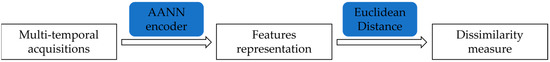
Figure 1.
Main steps of the testing phase.
2.1. Dataset
Sentinel-2 is a Copernicus Programme mission developed by the European Space Agency (ESA) with an open data distribution policy. It comprises a constellation of two polar-orbiting satellites with wide swath width and a combined revisit time of five days at the equator, which monitor variability in land surface conditions. Data are acquired in 13 spectral bands spanning from the visible and the near infrared to the short-wave infrared. The spatial resolution varies from 10 m to 60 m, depending on the spectral band [27].
To have a dataset of sufficient size to train the AANN, 36 multispectral images with the processing level 1C (top-of-atmosphere reflectance) of urban and suburban areas worldwide were collected. Images were obtained through the Copernicus Open Access Hub [30]. The considered scenes are approximately 700 × 700 pixels in size and do not contain clouds or haze. Figure 2 shows two sample images in RGB composition. This dataset was integrated with the Onera Satellite Change Detection (OSCD) dataset, which is similarly composed of 24 Sentinel-2 multispectral images acquired in different locations around the world [31]. For each location, registered pairs of images at a temporal distance of 2–3 years are provided, so the image for the same area is available for the time t1 and for the time t2. The pixel-level change ground truth is given for 14 images, and the annotated changes focus on urban changes, such as buildings or roads, while natural changes, such as vegetation, sun exposure and brightness condition, are ignored. A sample image pair and its corresponding ground truth are shown in Figure 3.
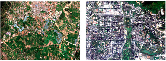
Figure 2.
Samples from the Sentinel-2 dataset, 10 m spatial resolution (RGB).
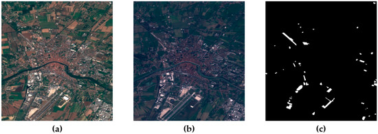
Figure 3.
Sample from the OSCD dataset: (a) image acquired at time t1 (RGB); (b) image acquired at time t2 (RGB); (c) ground truth (changed areas are shown in white).
Thus, the final dataset consists of 60 multispectral images. Among these, 5 labelled OSCD images were used to test the final performance of the algorithm.
2.2. Description of the Reference Data
The OSCD ground truth images were generated manually by comparing the true colour composition of each image pair. However, as explained in Section 2.1, in this case natural changes (e.g., vegetation growth or sea tides) are not considered [31]. For this reason, another level of reference truth was generated for evaluation of the results. This has been obtained by applying a change vector analysis (CVA) to the original pair of images. CVA is a widely used change detection technique for optical images because it can produce detailed information and can process any number of input bands. In the procedure, the pixelwise difference in spectral measurements is computed and all difference values greater than a predefined threshold are labelled as changed pixels [13,24].
In CVA, the threshold determination is a critical task, and, to this end, an empirical method based on the direct observation of the test image pairs, already proposed in [32], has been considered. In more detail, the five labelled OSCD image pairs belonging to the test set were considered first. For each image pair, all areas showing significant changes were extracted. Here, we included both artificial changes (already made available by the OSCD dataset) and natural changes that have been detected by additional CVA. An example of an additional changed area is shown within the yellow polygon in Figure 4. For each changed area, the average pixel value at time t1 and at time t2 and the difference between such average values were computed. The threshold was then determined in order to minimize the number of false positives and false negatives obtained on the described set of examples. The procedure was repeated for the three bands: R, G and B. It was found that, ignoring small alterations, the selected thresholds were sensitive enough to highlight the relevant changes. Finally, the determined thresholds were applied on the entire pixelwise difference images to generate the reference binary maps.
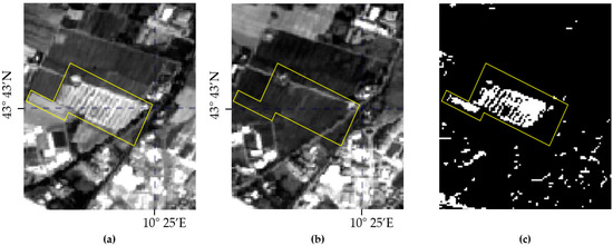
Figure 4.
Example of an area used for the threshold determination: (a) the average value of the changed pixels in the yellow polygon is 1700 at time t1 and (b) 740 at time t2. (c) Binary image obtained with 1000 as threshold value (changed areas are shown in white).
The CVA depends on the analyst’s identification of suitable factors; however, it can offer a reliable benchmark comparison, and a meaningful example is provided by the test image reported in Figure 3. The difference between the OSCD and CVA ground truth images are shown in Figure 5: the large white areas in Figure 5b highlight the modifications in land cover that are not reported in Figure 5a. Indeed, the ground truth image obtained by means of CVA was specifically made to point out these alterations.
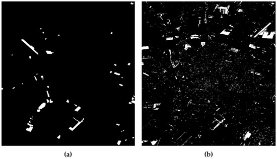
Figure 5.
Comparison between (a) OSCD and (b) CVA ground truth images for test image shown in Figure 3 (change areas are shown in white).
2.3. AANN
AANNs are multi-layer perceptron networks, i.e., feedforward NNs, composed of layers of units that have nonlinear activation functions. As shown in Figure 6, the number of nodes in the input layer coincides with the number of nodes in the output layer. Unlike a standard topology, an AANN uses three hidden layers, including an internal bottleneck layer of smaller dimension than either input or output. Therefore, the network has a symmetrical structure that can be viewed as two successive functional mappings: the first half of the network maps the input vector to a lower dimensional subspace via the encoder module, while the second decodes it back via a decoder module. The dimension of the lower subspace is determined by the number of units in the bottleneck layer that plays the key role in the functionality of the AANN: data compression caused by the network bottleneck may force hidden units to represent significant features in the input data [8]. The number of neurons to be considered in the hidden layers is a critical choice, in particular in the bottleneck layer: a small number of units means a significant dimensionality reduction in the input data, but, if the number is too small, the input-output associative capabilities of the net are too weak.
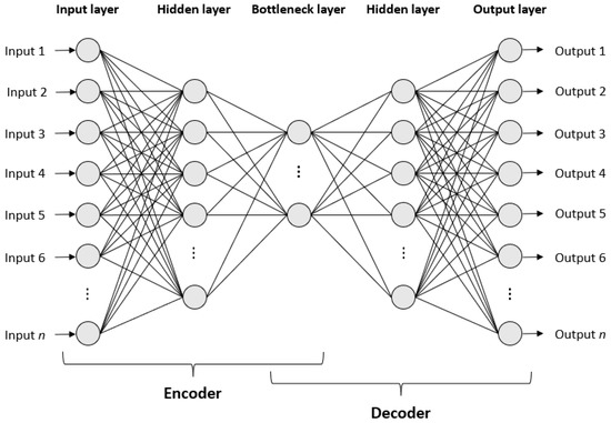
Figure 6.
AANN topology.
Further details regarding the AANN architecture used in this study are described in Section 2.5.
2.4. DWT
The DWT algorithm was chosen as a benchmark technique for performance analysis because it is broadly used for image compression purposes, for example, in the JPEG2000 compression standard and also for remote sensing images in most Earth observation satellites [19,33]. The two-dimensional DWT decomposes the input image along the rows and along the columns into high frequency and low frequency parts, called low-low (LL), low-high (LH), high-low (HL), and high-high (HH) sub-bands; thus, each decomposed level consists of four sub-bands of coefficients. The LL sub-band represents the low pass filtering along rows and columns of the input image, and it is recursively used to obtain the subsequent level of decomposition, until reaching the predefined number of decomposition level. The n-th decomposition level is the approximation of the input image [29,34].
2.5. Dimensionality Reduction
The dataset described in Section 2.1 was pre-processed. The red, green and blue bands (namely, band 2, band 3 and band 4) were considered for each image, having a finer spatial resolution of 10 m. Moreover, they have been proved suitable in various change detection techniques, especially the red band, in both vegetated and urban environments [24].
After co-registration of each pair, the images were divided into sub-images, i.e., patches, with a dimension of pixels for a total of 55,191 patches. Each patch was normalized in the 0–1 interval, and the same procedure was done for the images in the test set [35]. We decided to set the goal of reducing the data dimensionality of one order; therefore, we aimed to represent each sub-image with 32 components. On one side, this clearly defines a benchmark for the level of reduction, which can be useful for future studies; on the other side, it is consistent with on-line implementations.
The training dataset was split into two distinct parts, training and validation set, with a proportion of 80% and 20%, respectively as summarized in Table 1. The AANN training performance was evaluated both on the training set and on the validation set because, according to the early stopping algorithm, the training of the net was stopped when the error on the validation set reaches its minimum [11].

Table 1.
Train and validation distribution.
The final AANN architecture resulted in the following topology: 1024 units in the input and output layers, 128 units in the encoded and decoded layer and 32 units in the bottleneck layer. The number of 128 units stems from a trial-and-error approach in which it was observed that other lengths of these intermediate layers did not improve the final performance. The model was developed in Python with TensorFlow2 and Keras libraries and trained with the mean squared error (MSE) loss function and Adam optimizer [36]; the batch size was set to 64. A backpropagation algorithm was applied for the weights matrix update [37]. Figure 7 shows the trend of the loss function for the training and validation sets.
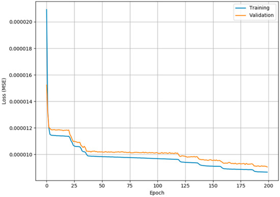
Figure 7.
Loss function trend.
In the DWT dimensionality reduction procedure, the input image patches are similarly obtained by splitting the test images into sub-images of size pixels. The Haar filter was chosen as the mother wavelet, and the number for the decomposition level was set to 2 [33], as shown in Figure 8.
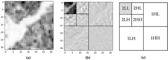
Figure 8.
(a) Original patch; (b) 2-level DWT; (c) DWT level and sub-bands.
Figure 9 aims at comparing the patch reconstruction with both techniques AANN and DWT. Figure 9a,d shows the original test patches, extracted from the dataset at the R band (band number 4), at times t1 and t2; the significant variation in the lower left corner of the sub-image can be noted. Figure 9b,e, in the middle, illustrates the reconstructed patch obtained as the output of the AANN, after propagation of the original patch through the bottleneck layer. In Figure 9c,f, the DWT reconstruction is shown; only the first 32 coefficients of DWT were extracted, setting the remaining ones to zero.
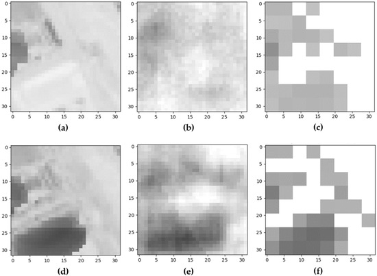
Figure 9.
Comparison between the reconstructed images: (a) original patch at time t1; (b) patch reconstruction through the AANN model; (c) patch reconstruction through DWT; (d) original patch at time t2; (e) patch reconstruction through the AANN model; (f) patch reconstruction through DWT.
2.6. Dissimilarity Measurements
Figure 10 shows the main procedure steps for change detection at the patch level. The smaller representation, i.e., the patch vectorial representation (PVR), of the input patches associated with time t1 was obtained by means of the AANN or the DWT techniques. In particular, only the encoder stage of the AANN is involved in this step, with the output represented by the bottleneck layer. Thus, the AANN input is a vector of length 1024, which is compressed into a smaller vector of length 32. Afterwards, the same procedure was done for the patch associated with time t2. Then, the dissimilarity between the two obtained PVRs was computed.
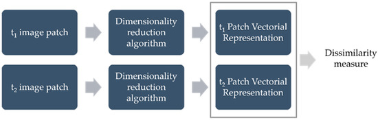
Figure 10.
Scheme of the change detection.
In particular, the Euclidean distance (ED), defined according to the following expression, was considered:
where is the index of the vector element, and , are the -th patches associated with time t1 and with time t2, respectively.
3. Results
Although the procedure previously described was separately applied to the three bands R, G and B, in this section only the results of the R band will be shown. Indeed, this band is recognized to have, in general, greater sensitivity to variations, and the results achieved using the other two bands were less accurate [24].
In Figure 11, two images extracted from the test set are shown. Figure 11a1,a2 represent an area mainly covered by vegetation. The main changed elements regard the land cover with some variations in buildings and roads. The ground truth is represented at two levels: in Figure 11b, it relies on the OSCD dataset, while, in Figure 11c, it stems from the CVA technique explained in Section 2.2. In both cases, the changed areas are shown in white. Similarly, Figure 11d1,d2,e,f represent another pair of images with the associated ground truth, but, in this latter case, the images show mainly built-up areas.
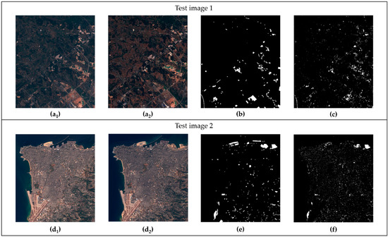
Figure 11.
Examples 1 and 2 from test dataset: (a1,d1) images acquired at the time t1 in RGB composition; (a2,d2) images acquired at the time t2 in RGB composition; (b,e) OSCD ground truth; (c,f) CVA ground truth (changed areas are shown in white).
3.1. Qualitative Assessment
We have seen that the methodology is applied at the patch level. For the performance analysis, the patches obtained from the ground truth images were therefore divided into three categories: patches without changes, patches with more than 10% of pixels changed (i.e., out of 1024 total pixels, 102 are changed) and patches with less than 10% of pixels changed. The percentage of 10% was chosen because it represents the average extension of the changed areas within the patch. This allowed for analysis of the performance, either on patches with significant changes or on patches with smaller changes. Moreover, it should be specified that patches reporting less than 1% of pixels as changed (i.e., out of 1024 total pixels, 10 are changed) were considered no change patches. This choice allows for discarding of the patches with cropped changed areas from the OSCD ground truth and of the patches with irrelevant alterations from the CVA change ground truth. For each pair of patches, the ED values were normalized in the 0–1 interval and were compared with their respective ground truth labelling.
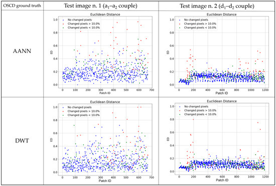
In Figure 12, the graphs report, for the test image pairs shown in Figure 11 and for both the AANN and DWT approaches, the ED values on the y-axis, while the patch’s identifying number is reported on the x-axis. Each point is then colored according to the corresponding OSCD ground truth: patches without changes are shown in blue, patches with more than 10% of pixels changed are in red and patches with less than 10% of pixels changed are in green. We see that for both methods, the PVRs associated with no change patches are mainly localized in the lower part of the graph, while the PVRs related to a high number of changed pixels are in the upper area. Few PVRs in the green class (changed pixels below 10%) report ED values near zero, but this never happens for examples belonging to the red class. The misclassified samples seem to grow with the DWT dimensionality reduction. The graphs also point out the different response of the two considered images. Test image number 2 (couple (d) in Figure 11) performed better with both the AANN and DWT, and a clearer distinction between blue and red markers can be observed. On the contrary, test image number 1 (couple (a) in Figure 11) shows some no change PVRs at high ED values. However, it has to be remembered that the OSCD ground truth does not consider natural changes, such as vegetation growth.
In an ideal setting, the ED values related to a no change condition should be the lowest and grow as the number of changed pixels increases. This trend is evaluated in Figure 13, which reports the correlation between the number of changed pixels in a ground truth patch and the respective ED. As for Figure 12, the graphs are shown for the AANN and DWT algorithms. Indeed, the presence of a linear correlation can be observed, especially for the AANN method. It also has to be noted that the linear trend is disturbed by the significant number of the no change patches, and this situation is enhanced in test image number 1.
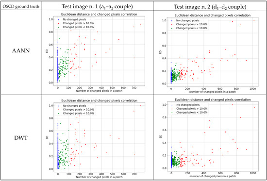
Figure 13.
Correlation between the number of changed pixels in a ground truth patch (x-axis) and the corresponding ED value (y-axis) for the test images 1 in Figure 11a1,a2 (left) and the test images 2 in Figure 11d1,d2 (right). Each marker is colored according to the change condition in the OSCD ground truth patch.
The same analysis was repeated considering the ground reference obtained with the CVA method. The corresponding graphs are shown in Figure 14 and Figure 15. Here, the EDs related to a condition of significant change (markers in red) are distinctly separated from the unchanged ones, especially in test image 2. Figure 15, compared to the previous case, shows a higher linear correlation between the number of changed pixels and the ED values. The performance is generally better with respect to the OSCD ground-truth. This could be expected because, in this case, all types of changes are considered in the ground truth, and this is more consistent with the sensitivity characteristics expressed by the ED measurement. However, the qualitative assessment carried out so far suggests that the PVR can be effective for the distinction among patches with relevant changes and patches with small or no changes.
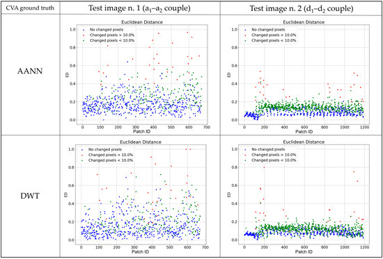
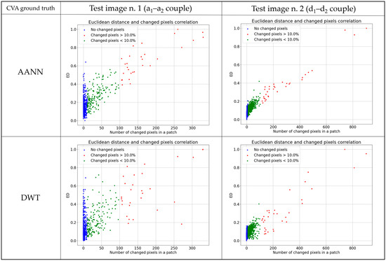
Figure 15.
Correlation between the number of changed pixels in a ground truth patch (x-axis) and the corresponding ED value (y-axis) for test image 1 in Figure 11a1,a2 (left) and test image 2 in Figure 11d1,d2 (right). Each marker is colored according to the change condition in the CVA ground truth patch.
3.2. Quantiative Performance Analysis
Typical metrics for image classification quantitative performance analysis are:
where:
- TP = true positives, i.e., samples labelled as changed (red markers) and correctly predicted by the model;
- TN = true negatives, i.e., samples labelled as not changed (blue markers) and correctly predicted by the model;
- FP = false positives, i.e., samples labelled as not changed (blue markers) and wrongly predicted as changed by the model;
- FN = false negatives, i.e., samples labelled as changed (red markers) and wrongly predicted as not changed by the model.
In the metrics computations, samples related to patches with less than 10% of pixels changed (i.e., green markers) were discarded.
As highlighted in the ground truth images, the number of changed pixels is significantly lower than the number of unchanged ones, and this class imbalance was considered during the results evaluation. In the case of an unbalanced dataset, accuracy is not useful, while the F1 score represents a proper measure as a combination between precision and recall. The receiver operating characteristic (ROC) curve is also a valid method for evaluating the performance of an algorithm. It plots the recall against the FPR, and the area under the curve (AUC) measures the performance of the model for all possible change thresholds. The AUC ranges from 0.5 for a random classifier to 1 for a perfect classifier. Figure 16 and Figure 17 show the ROC curve obtained by validating with OSCD and CVA ground truth images, respectively, for test images 1 and 2 in Figure 11.
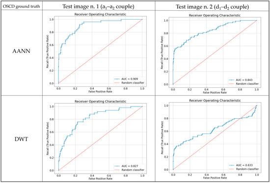
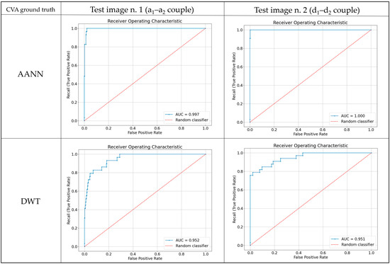
Figure 16 highlights that the lowest AUC value occurs for test image number 2, in the DWT case. With the AANN algorithm, the value improves by approximately 0.2. Test image number 1 exhibits better AUC values; the best is 0.909 for the AANN algorithm. By validating with the CVA (Figure 17), the values increase, reaching almost 1 for test image 2 with the AANN algorithm, but the other cases also reach high AUC values.
Table 2 summarizes the results obtained for test image number 1, shown in Figure 11(a1,a2), validated with the OSCD and CVA reference images. The results obtained with the AANN and DWT techniques were compared; the table also reports the AUC values. The change detection with AANN reduction performed better than DWT, as already demonstrated in Figure 12 and Figure 14. F1 achieves 0.86 with CVA validation and AANN reduction, which is more than 0.2 higher than DWT. The result also increases by the same value when validating with OSCD reference image, although, in this latter case, the best absolute value of F1 is 0.6. Recall represents an important metric to analyze, since it provides a measure of the number of missed changes, and these are the main focus of a change detection algorithm. Recall doubles by performing reduction with the AANN, with both OSCD and CVA validations.
Table 2.
Results for test image 1.
However, in an operational scenario, the threshold value should be previously defined, in order for the algorithm to run automatically. The choice of an optimum general value can be a very difficult task because it definitely depends on the land cover contained in the image; a scene with a prevalence of urban areas would certainly provide an optimum threshold value different from that of a rural one. To address this issue, we selected from the dataset the two most similar images in terms of land cover: test image number 1 (shown in Figure 11a1,a2) was compared to test image number 3 (shown in Figure 3). Based on the recall scores, we selected from image number 1 a threshold value of 0.4 as the optimum one, and we used the same value to evaluate the change detection results on image 3. The final scores on test image 3 are reported in Table 3 for both the OSCD and the CVA datasets and always consider the performance obtained with the DWT as a benchmark.
Table 3.
Results for test image 3.
The main change elements in test image number 3 are seasonal land cover variations that are not labelled in the OSCD ground truth image: This factor affects the results that reported lower performance, as shown in Table 3. The metrics rise sharply considering the comparison with CVA image, as shown in the table. In fact, the ground truth image obtained via the CVA was specifically made to point out these alterations. In this case, F1 reaches 0.92 with an AANN reduction.
Finally, it must be underlined that the developed algorithm is not heavy in terms of computational requirements. It was performed on NVIDIA® GeForce® GTX 1650 Max Q GPU with 4 GB RAM. During the test phase, the time taken to open a couple of satellite images with size of 772 × 902 pixels, divide them in patches, normalize their values and return their encoded representation was 9.8 s and required 25.79 MB of RAM. The training weights of the AANN encoder part require less than 3 MB for storage.
4. Discussion
The method proposed here aims to develop a change detection technique with a compressed representation of the two considered images. The smaller representation can be obtained by means of an AANN or DWT, but PVRs extracted with an AANN led to better results in change detection.
The results were validated by means of OSCD ground truth, but, as highlighted in Section 2.1, these images report only man-made changes, leaving out the natural changes. This characteristic negatively impacts the results, moreso for test images showing a natural environment than those with an urban setting. Therefore, validation of images obtained by means of CVA were also considered. As described in Section 2.2, this method depends on the analyst’s sensitivity but was demonstrated to be effective in this case, overcoming the critical issues related to OSCD ground truth.
Compared to the study described in [25], our work proposed a method focused on detecting any type of change and was tested on Sentinel-2 images that were easy to access and use. Additionally, the detection was performed on a compressed representation of the original acquisition. In [16], Kalinicheva et al. used NNs and Spot-5 images at 10 m of spatial resolution, although the algorithm can be applied to any type of satellite acquisitions. The changed areas were highlighted through an image pixel-based subtraction. In this case, compression of the image is not performed to reduce the amount of data but to apply the subtraction method. Indeed, subtraction works fine on lower resolution images, but the pixelwise analysis may not be compliant with on-board processing requirements. Zhao et al. [17] used multi-temporal hyperspectral images as the input dataset and two NN models. The features extracted by the first network are considered additional input for the second NN, which performs the change detection. They achieved more than 95% accuracy, but the complexity of the scheme does not seem developed to be run on-board.
The testing phase led to promising results, as shown in the figures in Section 3.1, although it revealed the criticality related to the definition of a unique threshold to automatically perform the change detection. In fact, this value strictly depends on the scene depicted in the image. For this reason, numerical results were evaluated for two images of the test set that are similar in terms of land cover. By validating with the CVA, the AANN reached higher score values than the OSCD ground truth, and the gap with the DWT algorithm is sharply marked for test image 3. Generally, the results obtained by validating with the CVA were significantly better than the ones obtained with the OSCD.
5. Conclusions
In a scenario where the demand for on-board processing to be run on space payloads is increasing more and more to limit both bandwidth and data storage, this work proposes a new method for on-board change detection based on NN. In particular, an AANN extracts the image features, which are then used for a CVA. AANNs are characterized by a very light architecture; hence, they are particularly suitable for on-board operations.
In this study, the change detection algorithm was applied to Sentinel-2 images. Moreover, for performance analysis purposes, a standard image compressor based on DWT was also considered as a benchmark. The algorithms perform dimensionality reduction in multi-temporal input image patches by reducing their initial size into smaller representative vectors. A dissimilarity measure, i.e., the ED, was computed to indicate the probabilities of change.
The main contributions of this work can be summarized in three aspects: First, it shows the capability of AANNs in image compression and reconstruction. As detailed in Section 2.5, the AANN achieved better results in reconstructing images than other well-known techniques, such as the DWT. Second, while most of the current change detection approaches use deep learning schemes [38], our algorithm provides an innovative shallow neural network technique using compressed representation. Lastly, the procedure presented here was designed and developed to be run on-board, and the on-board processing is currently another relevant topic. The computing resources and the memory required to store the training weights are comparable to those typically available on-board, as described in Section 1. The results demonstrated that for change detection purposes, image encoding by means of AANNs led to better achievements than the DWT and required low-level computing resources in the test phase, which could then be executed on-board. The results improved up to 0.2 in terms of the F1 score. The classification accuracy between the classes change and no change is strictly affected by the input dataset and the validation images. Indeed, datasets for change detection analysis are typically characterized by class imbalance and limited availability of ground truth images. Despite this, a promising distinction between EDs related to areas reporting significant changes and those for no change areas was shown, reaching an F1 score of 0.9.
Further research will investigate the tailoring of the method for SAR data, since they allow the implementation of the algorithm in any weather condition and during the night.
Author Contributions
Conceptualization, G.G.; methodology, G.G. and F.D.F.; software, G.G.; validation, G.G., F.D.F. and G.S.; formal analysis, G.G., F.D.F. and G.S.; investigation, G.G.; resources, G.G., F.D.F. and G.S.; data curation, G.G.; writing—original draft preparation, G.G. and F.D.F.; writing—review and editing, F.D.F. and G.S.; visualization, F.D.F.; supervision, F.D.F. and G.S.; project administration, F.D.F. and G.S.; funding acquisition, F.D.F. and G.S. All authors have read and agreed to the published version of the manuscript.
Funding
This research received no external funding.
Data Availability Statement
Not applicable.
Conflicts of Interest
The authors declare no conflict of interest.
References
- Poursanidis, D.; Chrysoulakis, N. Remote Sensing, natural hazards and the contribution of ESA Sentinels missions. Remote Sens. Appl. Soc. Environ. 2017, 6, 25–38. [Google Scholar] [CrossRef]
- Kussul, N.; Lavreniuk, M.; Skakun, S.; Shelestov, A. Deep Learning Classification of Land Cover and Crop Types Using Remote Sensing Data. IEEE Geosci. Remote Sens. Lett. 2017, 14, 778–782. [Google Scholar] [CrossRef]
- Del Frate, F.; Pacifici, F.; Solimini, D. Monitoring Urban Land Cover in Rome, Italy, and Its Changes by Single-Polarization Multitemporal SAR Images. IEEE J. Sel. Top. Appl. Earth Obs. Remote Sens. 2008, 1, 87–97. [Google Scholar] [CrossRef]
- Qi, B.; Shi, H.; Zhuang, Y.; Chen, H.; Chen, L. On-Board, Real-Time Preprocessing System for Optical Remote-Sensing Imagery. Sensors 2018, 18, 1328. [Google Scholar] [CrossRef] [Green Version]
- Sweeting, M.N. Modern Small Satellites-Changing the Economics of Space. Proc. IEEE 2018, 106, 343–361. [Google Scholar] [CrossRef]
- Penalver, M.; Del Frate, F.; Paoletti, M.; Haut, J.; Plaza, J.; Plaza, A. Onboard payload-data dimensionality reduction. In Proceedings of the IEEE International Geoscience and Remote Sensing Symposium (IGARSS), Fort Worth, TX, USA, 23–28 July 2017. [Google Scholar]
- Trautner, R.; Vitulli, R. Ongoing Developments of Future Payload Data Processing Platforms at ESA; OBPDC: Toulouse, France, 2010. [Google Scholar]
- Zhang, L.; Zhang, L.; Du, B. Deep Learning for Remote Sensing Data: A Technical Tutorial on the State of the Art. IEEE Geosci. Remote Sens. Mag. 2016, 4, 22–40. [Google Scholar] [CrossRef]
- Shi, W.; Zhang, M.; Zhang, R.; Chen, S.; Zhan, Z. Change Detection Based on Artificial Intelligence: State-of-the-Art and Challenges. Remote Sens. 2020, 12, 1688. [Google Scholar] [CrossRef]
- Kramer, M.A. Autoassociative Neural Networks. Comput. Chem. Eng. 1991, 37, 313–328. [Google Scholar] [CrossRef]
- Licciardi, G.A.; Del Frate, F. Pixel Unmixing in Hyperspectral Data by Means of Neural Networks. IEEE Trans. Geosci. Remote Sens. 2011, 49, 4163–4172. [Google Scholar] [CrossRef]
- Fasano, L.; Latini, D.; Machidon, A.; Clementini, C.; Schiavon, G.; Del Frate, F. SAR Data Fusion Using Nonlinear Principal Component Analysis. IEEE Geosci. Remote Sens. Lett. 2019, 17, 1543–1547. [Google Scholar] [CrossRef]
- Saha, S.; Bovolo, F.; Bruzzone, L. Unsupervised Deep Change Vector Analysis for Multiple-Change Detection in VHR Images. IEEE Trans. Geosci. Remote Sens. 2019, 57, 3677–3693. [Google Scholar] [CrossRef]
- Asokan, A.; Anitha, J. Change detection techniques for remote sensing applications: A survey. Earth Sci. Inform. 2019, 12, 143–160. [Google Scholar] [CrossRef]
- Khelifi, L.; Mignotte, M. Deep Learning for Change Detection in Remote Sensing Images: Comprehensive Review and Meta-Analysis. IEEE Access 2020, 8, 126385–126400. [Google Scholar] [CrossRef]
- Kalinicheva, E.; Sublime, J.; Trocan, M. Neural network autoencoder for change detection in satellite image time series. In Proceedings of the 25th IEEE International Conference on Electronics, Circuits and Systems (ICECS), Bordeaux, France, 9–12 December 2018. [Google Scholar]
- Zhao, C.; Cheng, H.; Feng, S. A Spectral–Spatial Change Detection Method Based on Simplified 3-D Convolutional Autoencoder for Multitemporal Hyperspectral Images. IEEE Geosci. Remote Sens. Lett. 2021, 19, 1–5. [Google Scholar] [CrossRef]
- Yao, Y.; Jiang, Z.; Zhang, H.; Zhou, Y. On-Board Ship Detection in Micro-Nano Satellite Based on Deep Learning and COTS Component. Remote Sens. 2019, 11, 762. [Google Scholar] [CrossRef] [Green Version]
- Zhang, Z.; Iwasaki, A.; Xu, G.; Song, J. Cloud detection on small satellites based on lightweight U-net and image compression. J. Appl. Remote Sens. 2019, 13, 026502. [Google Scholar] [CrossRef]
- Del Rosso, M.P.; Sebastianelli, A.; Spiller, D.; Mathieu, P.P.; Ullo, S.L. On-Board Volcanic Eruption Detection through CNNs and Satellite Multispectral Imagery. Remote Sens. 2021, 13, 3479. [Google Scholar] [CrossRef]
- Diana, L.; Xu, J.; Fanucci, L. Oil Spill Identification from SAR Images for Low Power Embedded Systems Using CNN. Remote Sens. 2021, 13, 3606. [Google Scholar] [CrossRef]
- Danielsen, A.S.; Johansen, T.A.; Garrett, J.L. Self-Organizing Maps for Clustering Hyperspectral Images On-Board a CubeSat. Remote Sens. 2021, 13, 4174. [Google Scholar] [CrossRef]
- Rapuano, E.; Meoni, G.; Pacini, T.; Dinelli, G.; Furano, G.; Giuffrida, G.; Fanucci, L. An FPGA-Based Hardware Accelerator for CNNs Inference on Board Satellites: Benchmarking with Myriad 2-Based Solution for the CloudScout Case Study. Remote Sens. 2021, 13, 1518. [Google Scholar] [CrossRef]
- Lu, D.; Mausel, P.; Brondìzio, E.; Moran, E. Change detection techniques. Int. J. Remote Sens. 2004, 25, 2365–2407. [Google Scholar] [CrossRef]
- Spigai, M.; Oller, G. On-Board Change Detection with Neural Networks. In Proceedings of the International Archives of Photogrammetry Remote Sensing and Spatial Information Sciences, Denver, CO, USA, 10–15 November 2002. [Google Scholar]
- Kara, C.; Aslan, A.B.; Canberi, M.H. Test Software for National Satellite On-Board Computer. In Proceedings of the 2020 Turkish National Software Engineering Symposium (UYMS), Istanbul, Turkey, 7–9 October 2020. [Google Scholar]
- Drusch, M.; del Bello, U.; Carlier, S.; Colin, O.; Fernandez, V.; Gascon, F.; Hoersch, B.; Isola, C.; Laberinti, P.; Martimort, P.; et al. Sentinel-2: ESA’s Optical High-Resolution Mission for GMES Operational Services. Remote Sens. Environ. 2012, 120, 25–36. [Google Scholar] [CrossRef]
- Giuffrida, G.; Diana, L.; De Gioia, F.; Benelli, G.; Meoni, G.; Donati, M.; Fanucci, L. CloudScout: A Deep Neural Network for On-Board Cloud Detection on Hyperspectral Images. Remote Sens. 2020, 12, 2205. [Google Scholar] [CrossRef]
- Chowdhury, M.M.H.; Khatun, A. Image Compression Using Discrete Wavelet Transform. IJCSI Int. J. Comput. Sci. Issues 2012, 9, 327–330. [Google Scholar]
- Copernicus Open Access Hub. Available online: https://scihub.copernicus.eu/ (accessed on 3 April 2020).
- Daudt, R.; le Saux, B.; Boulch, A.; Gousseau, Y. Urban Change Detection for Multispectral Earth Observation Using Convolutional Neural Networks. In Proceedings of the IEEE International Geoscience and Remote Sensing Symposium (IGARSS), Valencia, Spain, 22–27 July 2018. [Google Scholar]
- Singh, S.; Talwar, R. Performance analysis of different threshold determination techniques for change vector analysis. J. Geol. Soc. India 2015, 86, 52–58. [Google Scholar] [CrossRef]
- Celik, T. Multiscale Change Detection in Multitemporal Satellite Images. IEEE Geosci. Remote Sens. Lett. 2009, 6, 820–824. [Google Scholar] [CrossRef]
- Ahuja, S.N.; Biday, S.; Ragha, L. Change Detection in Satellite Images Using DWT and PCA. Int. J. Eng. Assoc. 2018, 2, 76–81. [Google Scholar]
- Bishop, C.M. Neural Networks for Pattern Recognition; Oxford University Press: Oxford, UK, 1995. [Google Scholar]
- Kingma, D.P.; Ba, J.L. Adam: A method for stochastic optimization. In Proceedings of the International Conference on Learning Representations (ICLR), San Diego, CA, USA, 7–9 May 2015. [Google Scholar]
- Li, J.; Cheng, J.-h.; Shi, J.-y.; Huang, F. Brief Introduction of Back Propagation (BP) Neural Network Algorithm and Its Improvement. Adv. Comput. Sci. Inf. Eng. 2012, 169, 553–558. [Google Scholar]
- Saha, S.; Ebel, P.; Zhu, X.X. Self-supervised multisensor change detection. IEEE Trans. Geosci. Remote Sens. 2022, 60, 4405710. [Google Scholar] [CrossRef]
Publisher’s Note: MDPI stays neutral with regard to jurisdictional claims in published maps and institutional affiliations. |
© 2022 by the authors. Licensee MDPI, Basel, Switzerland. This article is an open access article distributed under the terms and conditions of the Creative Commons Attribution (CC BY) license (https://creativecommons.org/licenses/by/4.0/).