CloudSatNet-1: FPGA-Based Hardware-Accelerated Quantized CNN for Satellite On-Board Cloud Coverage Classification

Abstract

CubeSats, the nanosatellites and microsatellites with a wet mass up to 60 kg, accompanied by the cost decrease of accessing the space, amplified the rapid development of the Earth Observation industry. Acquired image data serve as an essential source of information in various disciplines like environmental protection, geosciences, or the military. As the quantity of remote sensing data grows, the bandwidth resources for the data transmission (downlink) are exhausted. Therefore, new techniques that reduce the downlink utilization of the satellites must be investigated and developed. For that reason, we are presenting CloudSatNet-1: an FPGA-based hardware-accelerated quantized convolutional neural network (CNN) for satellite on-board cloud coverage classification. We aim to explore the effects of the quantization process on the proposed CNN architecture. Additionally, the performance of cloud coverage classification by biomes diversity is investigated, and the hardware architecture design space is explored to identify the optimal FPGA resource utilization. Results of this study showed that the weights and activations quantization adds a minor effect on the model performance. Nevertheless, the memory footprint reduction allows the model deployment on low-cost FPGA Xilinx Zynq-7020. Using the RGB bands only, up to 90% of accuracy was achieved, and when omitting the tiles with snow and ice, the performance increased up to 94.4% of accuracy with a low false-positive rate of 2.23% for the 4-bit width model. With the maximum parallelization settings, the hardware accelerator achieved 15 FPS with 2.5 W of average power consumption (0.2 W increase over the idle state).

1. Introduction

Over the last decade, the Earth Observation (EO) industry has experienced a dramatic decrease in the cost of accessing space [1]. With the introduction of CubeSats, nanosatellites and microsatellites with wet mass up to 60 kg [2], the rapid development of remote sensing technologies was amplified [3]. As of 2021, more than 1500 CubeSats have been launched [4], and according to [5], it will increase up to a thousand satellites per year till 2028. Naturally, as the number of satellites grows, satellite imagery becomes readily available. Harvested data plays a significant role in various disciplines like environmental protection, agriculture engineering, land or mineral resource exploration, geosciences, or military reconnaissance [6,7]. In line with the amount of remote sensing data acquired, the bandwidth resources for the data transmission inclines to be overloaded. Therefore, new techniques for efficient bandwidth resources management must be investigated and developed.

Several studies estimate that approximately $67\%$ of the Earth’s surface is covered with clouds [6,8,9]. Consequently, most of the remote sensing imageries (RSI) will be contaminated by them, which devalues the quality of RSI and negatively affects the post-processing [6]. Cloudy conditions impair satellite sensor capabilities to obtain clear views of the Earth’s surface, and hence the quick and accurate detection of the cloudy images is necessary [6,10,11]. In general, the current methods for cloud coverage estimation or classification are mainly categorized into traditional and machine-learning-based approaches [12]. Traditional ones consist of threshold-based (fixed or adaptive), time differentiation, and statistical methods. The threshold-based approaches rely on a visible reflection and infrared temperature of the clouds, therefore its performance weakens on low-contrasted (cloud vs. surface) images [13,14,15]. Time differentiation methods effectively identify the changing pixel values as clouds in multi-temporal images, however, they do not consider changes in the top of atmosphere reflectance affected by floods [12,16]. Statistical methods combine spectral and spatial features extracted from RSIs with classical machine learning algorithms (support vector machine, decision tree), but they lack to obtain the desired results [17,18]. To sum up, traditional methods provide some capabilities of cloud detection, though, they are susceptible to the backgrounds, are non-universal and subjective [12].

A more efficient approach to cloudy image detection comprises convolutional neural networks (CNNs), simple linear iterative clustering, or semantic segmentation algorithms [12]. Especially attractive are CNNs, which provide state-of-the-art results for many different tasks, including image classification, segmentation, and object detection. This success is often achieved thanks to models with a huge number of parameters which means the large size and limited ability for the deployment on resource-constrained hardware. In recent years, there has been a tendency to deploy these models in line with the edge computing paradigm on resource-constrained hardware [12,19,20,21]. Various hardware accelerators are available on the market ranging from microcontrollers for smaller models to boards equipped with GPU, visual processing unit (VPU), or field-programmable gate array (FPGA). FPGA in particular provides interesting capabilities in terms of cost, flexibility, performance, and power consumption. A possible disadvantage is the long time to market in comparison to GPU or VPU solutions. 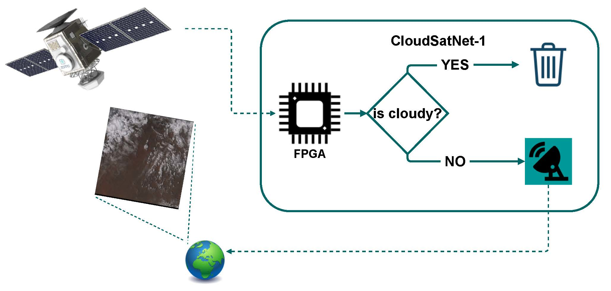Nevertheless, this gap is being closed by recent advancements in the hardware deployment of machine learning models [22,23] created in well-known machine learning frameworks like Pytorch or Tensorflow. Considering the payload limitations of the CubeSats, the optimal solution of the CubeSat’s cloud detection system is a system estimating RSI cloud coverage running directly on board. To reduce the costs and development time of such real-time detection systems, Commercial-Off-The-Shelf (COTS) components provide a favorable deployment option [24]. The crucial criterion for an onboard detection system is its power consumption, whereas the usual limit is below $5 \mathrm{W}$ and the ratio of the falsely discarded images below $2\%$ [12,19,20]. Generally, remote-sensing satellites can be equipped with a palette of sensors providing information in various bands. From the simplest one (RGB imageries) followed by multispectral imageries (usually a combination of RGB and near-infrared band (NIR)) to the hyperspectral imageries providing a complex spectrum of the sensed area [25,26].

In line with the above mentioned, Zhang et al. [27] introduced a lightweight CNN for cloud detection based on U-Net using red, green, blue, and infrared waveband images from the Landsat-8 dataset. Applying the LeGall-5/3 wavelet transform (4 levels) for dataset compression and processing time acceleration, the authors reported $94.3\%$ of overall accuracy running on an ARM-based platform. Similarly, in [28], the authors applied depthwise separable convolutions to compress the model of U-Net and accelerate the inference speed. The Study reported the best accuracy of $90.54\%$ verified on Landsat 8 remote sensing images. Another utilization of a lightweight MobU-Net trained on Landsat 8 dataset and using JPEG compression strategy was performed by [29]. The achieved overall accuracy was around $93.1\%$ for a model deployed on ARM9 processor on Zynq-7020 board. Maskey et al. [3] proposed an ultralight CNN designed for on-orbit binary image classification called CubeSatNet. The model was trained on BIRDS3 satellite images and deployed on ARM Cortex M7 MCU. An accuracy of 90% was achieved when classifying images as “bad” for cloudy, sunburnt, facing space, or saturated images and “good” in all other cases. A promising method for cloud detection using RS-Net and RGB bands exclusively was published by [30]. For model training, the Sentinel-2 dataset was used, and $76\%$ of accuracy was reported by the model deployed on an ARM-based platform. Another possibility is to use the Forwards Looking Imager instrument, which provides analysis of the upcoming environment of the satellite. This approach was examined in [31], testing various lightweight CNNs deployed on the Zynq-7020 board using FPGA. The authors reported high accuracy of $98\%$, however, 100 images only were used for testing. Vieilleville et al. [32] investigated the possibilities of the deep neural network (DNN) distillation process in order to reduce the size of DNN while accommodating efficiency in terms of both accuracy and inference cost. The authors were able to reduce the number of DNN parameters from several million to less than one with a minimal drop in performance in the image segmentation process.

To sum up, lightweight CNNs provide a competitive on-board cloud detection performance in comparison to the state-of-the-art deep convolutional neural networks, like CDNetV1 [6], CDNetV2 [10] or CD-FM3SFs [33]. CDNetV1 is a neural network for cloud mask extraction from ZY-3 satellite thumbnails with the accuracy of $96.47\%$ [6]. Its extended version, CDNetV2, focuses on adaptively fusing multi-scale feature maps and remedying high-level semantic information diluted at decoder layers to improve cloud detection accuracy with cloud-snow coexistence. The authors confirmed the robustness of the proposed method using validation on several other datasets like Landsat-8 or GF-1. Lately, Li et al. [33] introduced a lightweight network for cloud detection, fusing multiscale spectral and spatial features (CD-FM3SFs) using Sentinel-2A multispectral images. The best accuracy of $98.32\%$ was achieved using the CPU as a computational unit.

To the best of our knowledge, the CloudScout cloud detection method proposed by Giuffrida et al. [34] and later extended by Rapuano et al. [20] is the most related work to this study. The method was developed in the frame of the Phisat-1 ESA mission, which exploits a hyperspectral camera to distinguish between the clear and cloud-covered images. To reduce the bandwidth, the mission has set a criterion that only images that present less than $70\%$ of the cloudiness are transmitted to the ground. CloudScout was trained using Sentinel-2 hyperspectral data and achieved the $92\%$ of accuracy, $1\%$ of false positives with the power consumption of 1.8 W deployed on re-configurable Myriad-2 VPU by Movidius Intel [34]. Nevertheless, the authors identified multiple drawbacks due to the Myriad-2 design, which is not specifically suitable for the space environment (not based on a radiation-tolerant technology) [20]. Therefore, the authors extended their work and proposed an FPGA-based hardware accelerator for CloudScout CNN. The authors compared the Myriad-2 VPU with two FPGA boards: Zynq Ultrascale+ ZCU106 development board and Xilinx Kintex Ultrascale XQRKU060 radiation-hardened board. Results obtained by Zynq Ultrascale+ ZCU106 show that the FPGA-based solution reduced the inference time by 2.4 times (141.68 ms) but at the cost of 1.8 times greater power consumption (3.4 W) [20]. Inference time estimated for the Xilinx Kintex Ultrascale XQRKU060 board was 1.3 times faster (264.7 ms) in comparison with the Myriad-2 device, however, the power consumption was not reported.

Regarding the presented achievements of the related works and trends in the CubeSats development, we may expect a new era of smart nanosatellites equipped with reconfigurable, programmable hardware accelerators with an on-demand edge computing paradigm at payload level [3,12,19,20,27,28,29,31,34]. A usual aspect of the presented studies is the employment of multispectral or hyperspectral RSI for the cloud detection system. Generally, the bands’ composition of multi/hyperspectral RSI differs for individual missions, yet all are equipped with an RGB camera. Therefore, a cloud detection system built on RGB bands only may provide better portability for various missions independent of its multi/hyperspectral bands. In addition, the RGB cameras are several times cheaper and more convenient for short-term CubeSats missions. 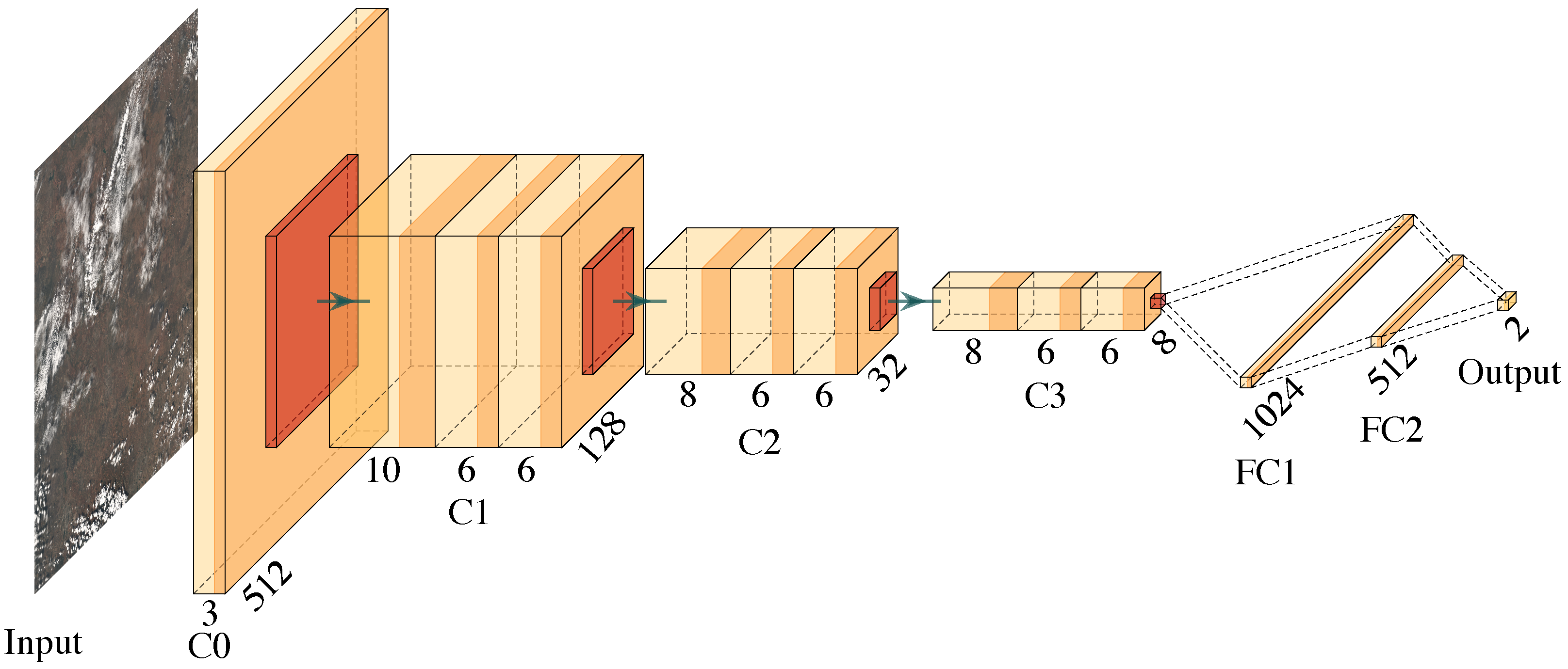To the best of our knowledge, we identified only three studies [20,21,31] that performed deployment and evaluation of the CNN-based cloud detection method on an FPGA-based platform. Hence, in the scope of this study, we would like to present CloudSatNet-1: an FPGA-based hardware-accelerated quantized CNN for satellite on-board cloud coverage classification. More specifically, we aim to:

• explore effects of quantization introduced to the proposed CNN architecture for cloud coverage classification,
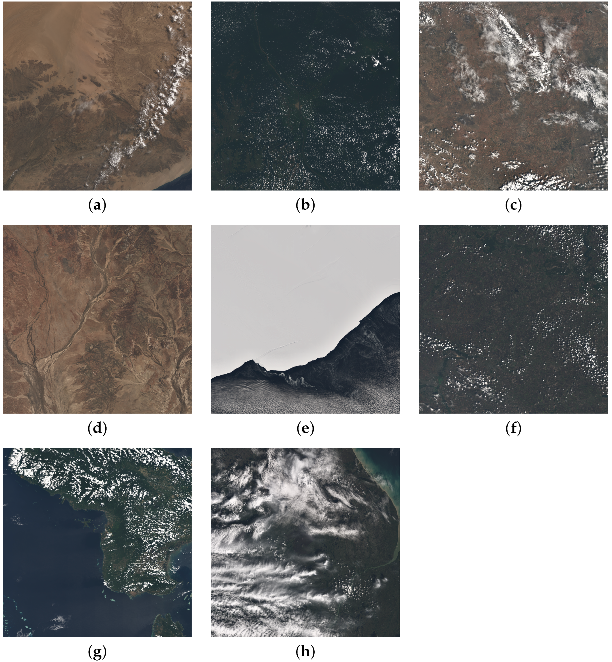
• investigate and optimize the performance of cloud coverage classification by biomes diversity and its false-positive identifications,
• explore hardware architecture design space to identify optimal FPGA resource utilization.

The rest of the paper is organized as follows. Section 2.1 describes the used dataset and its preprocessing. Methodology is described in Section 2.3. In Section 3, the results are summarized. The discussion can be found in Section 4 and the conclusions are drawn in Section 5.

2. Materials and Methods

2.1. Dataset

For the purpose of this study, the Landsat 8 Cloud Cover Assessment Validation data ($\mathrm{L}8$ biome dataset) [35] was used. The $\mathrm{L}8$ biome dataset offers a balanced cloud distribution and diverse sets of land and water cover, which makes it a suitable source of data for the proposed CNN-based classification model. The $\mathrm{L}8$ biome dataset was acquired by the Landsat 8 Operational Land Imager (OLI) and Thermal Infrared Sensor (TIRS) [36]. Furthermore, data are orthorectified and corrected for terrain relief using Level-1T processing [37].

The $\mathrm{L}8$ biome dataset consists of 96 scenes divided into 8 biomes. The scene size is 185 km by 180 km, and each scene contains 11 multispectral bands with a resolution of 30 m per pixel (except bands 8, 10, and 11, which are not used in this work). Manually annotated cloud coverage is stored as a cloud validation mask. The cloud validation mask is an image whose pixel values contain information about the level (or class) of cloudiness, interpreted using the following

Table 1. Interpretation of the $\mathrm{L}8$ biome dataset cloud mask pixel values [35].

Value	Interpretation
0	Fill
64	Cloud Shadow
128	Clear
192	Thin Cloud
255	Cloud

. The example of the scene image (natural color composition) from the $\mathrm{L}8$ biome dataset can be found in Figure 1a, with its respective cloud mask in Figure 1b.

Two cloud mask classes (thin cloud and cloud) are categorized as cloud pixels. From these pixels, the Cloud Cover Assessment (CCA) is computed as a ratio of cloud pixels to all pixels with values expressed in percentage [35]. The average CCA value for one scene is $48.35\%$. The distribution of the CCA values of the $\mathrm{L}8$ biome dataset scenes is shown in Figure 2. Scenes are categorized by their area of capture into biome classes by the International Geosphere-Biosphere Programme [38] into 8 following biomes: Barren (BA), Forest (FO), Grass/Crops (GC), Shrubland (SH), Snow/Ice (SI), Urban (UR), Water (WA), Wetlands (WE). They are distinguishable from each other by their visual properties, and they have various intensities of cloud to terrain contrast, which leads to different challenges for the cloud detection system working with RGB data. For example, the biomes with sharp cloud to terrain contrast, like Grass/Crops, have a large value of the derivative at the transition between terrain and cloud. Therefore Grass/Crops biome is easy to classify as cloud borders visibly stand out from the biome’s terrain. On the contrary, the other biomes like Snow/Ice have a terrain with cloud-like features, which may lead to a large number of false positives in classifier predictions as their terrain blends with clouds. Examples of image patches for each biome of the $\mathrm{L}8$ biome dataset are shown in Figure 3.

2.2. Data Preprocessing

The image patch for each scene is a natural color composite from the combination of bands B4 (red), B3 (green), and B2 (blue). Values in patch images are re-scaled from the range 0–65,535 to 0–255 using a MinMax normalization. Patch images in the $\mathrm{L}8$ biome dataset are georeferenced. The orbit path of the Landsat-8 does not go straight from south to north. The scene acquisition follows the orbit path of the satellite. Therefore the image appears to be rotated or tilted, like in Figure 4a. Redundant georeferencing information can be neglected when detecting clouds from satellite images. Next, the black (no-data) parts of the image need to be removed. The removal of the black parts consists of two steps. First, the image is rotated, so the actual image data are parallel to the whole scene image, as shown in Figure 4b. The rotation is using a nearest-neighbor interpolation method. Then, the image is cropped to lower resolution (from approx. 8000 × 8000 to approx. 6400 × 6400), so only image data are preserved, as illustrated in Figure 4c.

Image patch (with dimensions approx. 6400 × 6400 × 3) is cropped to 512 × 512 × 3 tiles, according the white lines in Figure 4c, omitting tiles at the edge that do not have full resolution. Each patch has a slightly different resolution after cropping, which causes a different number of generated tiles per patch (approx. 140). From 8 biomes each containing 12 scenes, there are in total 13,525 tiles. The original CCA values for the scene from Figure 2 do not apply to individual tiles. Generated tiles usually cover cloudy or cloud-free areas. This generates fewer tiles with balanced cloud coverage (or CCA value) in the final dataset (trade-off for creating many tiles from fewer image patches). Tiles with $\mathrm{CCA}\ge 70\%$ are categorized as cloud and the rest are categorized as non-cloud tiles. Each of the 13,525 tiles has been assigned a corresponding binary cloud coverage label. To preserve the evenly distributed cloud coverage in the train, validation and test dataset, the tiles from a single image patch are divided into 5 CCA quintiles: 0–20%, 20–40%, 40–60%, 60–80%, 80–100%. The distribution of the tiles and their CCA values per biome for the full $\mathrm{L}8$ biome dataset is visualized in Figure 5. The tiles from each patch CCA quintile are divided to train, validation and test datasets in the ratio 2:1:7, with the coherent variation of the biomes and their CCA values, as visualized in Figure 6. In this study, the reliability of the results and the model portability are prominent. Therefore, the testing dataset is dominant in comparison to the training or validation dataset. Moreover, more than 2700 tiles are considered a satisfactory quantity for the model training. Since the variation of the train, validation, and the test dataset is coherent, suppression or advantage of any of the biomes or the CCA quintile during the model training is not expected.

2.3. Methodology

The procedure is divided into three stages. First, the baseline model of CNN with floating point parameters is trained. Then the weights and activations of the model are quantized and the model is re-trained. The last step is the deployment of the model on FPGA to achieve high throughput and low power consumption suitable for on-board data processing on satellite. To be able to deploy a CNN on the edge there are many techniques how to reduce the model memory footprint such as pruning or quantization. In this work, the focus of interest is on quantization which replaces floating point operations and weight tensors with lower bit widths which are especially useful for FPGA where arbitrary precision data types can be implemented.

2.3.1. Quantized CNN

The main idea of this section is to introduce the quantization of CNN and its implementation for the purpose of this study.

Quantization in neural networks is a technique used for optimization which proved to produce great success in the recent years [39]. Its main focus is on reducing memory footprint and computation time by replacing floating point compute operations and storing tensor weights with lower bit widths. This is especially useful for resource-constrained applications. There are two ways how to introduce quantization to a neural network. The first one is to train the neural network with quantized parameters and the second one is a quantization of parameters after the model is trained with floating point precision. In the former case, the process is called quantization-aware training (QAT); in the latter, it is referred to as post-training quantization (PTQ). PTQ may disturb the model parameters and change the point to which it converged during the training with floating point precision. For this reason, QAT is used for the experiments conducted in this study and training with quantized model parameters is performed. For a more comprehensive review of the current state of quantization in neural networks refer to the recent survey [39].

The network was implemented using the Brevitas framework. Brevitas is a PyTorch library used for QAT of neural networks [40]. At the time of writing the PyTorch library supports the quantization as well but allows just reduction from 32-bit floating point to 8-bit integer [41]. Brevitas in comparison allows reducing the weight and activation bit widths to as low as 1-bit which enables the creation of binary neural networks (BNN) [42]. Another reason why the Brevitas library is used is that a model trained using Brevitas can be exported and used by the FINN framework for dataflow architecture acceleration (DFA) on Xilinx FPGAs [23]. The FINN framework is a compiler for feed forward DFA for deep neural networks (DNN) inference. When DFA is used, every layer of DNN is mapped to its own set of dedicated compute and memory resources [43] which mimics the topology of DNN. In FINN the performance and resource usage can be controlled with a concept called Folding. FINN uses what is called matrix-vector threshold units (MVTU) for convolutional and fully connected layers. There are three parameters that can be set: matrix-vector matrix-multiple vector (MMV) length, processing elements (PE), and single instruction multiple data (SIMD) lanes. Using these parameters, it is possible to control the throughput of the network with respect to resource utilization of the FPGA.

2.3.2. CloudSatNet-1 Architecture

In the following paragraph, the proposed CNN architecture and loss function used during the training period are described.

The proposed network architecture consists of 10 convolutional layers and 2 fully connected layers, their specific parameters are visualized in Figure 7. Each layer except the last layer uses the ReLU activation function and has no bias. The network starts with an initial convolutional layer which processes 512 × 512 × 3 uint8 input and continues with 3 sequences of 3 layers each. The input size was chosen to allow direct comparison with CloudScout architecture [34]. Each sequence middle layer has a lower number of filters to implement bottleneck for better generalization properties. After each sequence and initial layer, there is batch normalization and max pooling with kernel size of 4, this leads to the effective reduction of feature dimensions. The last fully connected layer outputs unnormalized probability for each class where the first class represents cloud presence below $70\%$ CCA in the image and the second class signals the presence of clouds above this threshold.

The loss function used for training the model was a modified binary cross entropy loss with an increased penalty for false positives (FP) errors shown in Equation (1). Penalty for FP errors is multiplied by a parameter $\alpha$ which is inspired by the approach reported in [34] where the authors showed a decrease in the number of FP errors while keeping accuracy on acceptable value when parameter $\alpha$ was set to 2.

$$F(y,\widehat{y})=-\frac{1}{\mathrm{N}}\sum _{i=1}^{\mathrm{N}}{y}_i·log\left({\widehat{y}}_i\right)+\alpha ·(1-y_i)·\log (1-{\widehat{y}}_i),$$

(1)

where y is the ground-truth label, $\widehat{y}$ is the predicted output of the network and $\alpha$ is a hyper-parameter to increase penalty for FP errors.

2.3.3. Quantization Process

First, the model with floating point precision is trained as a baseline. After sufficient accuracy has been achieved weight and activation bit widths are progressively reduced and the change in accuracy is observed. To fit the model on FPGA and achieve high throughput with acceptable accuracy and low power consumption, in this paper the focus of interest is bit widths of hidden layers lower or equal to 4. In all experiments, the same bit widths are used for weights and activations. The first and last layer of the neural network can be more sensitive to quantization [44,45,46], so they were quantized to 8 bits. The last fully connected layer has also a quantized bias term. It was observed by the preliminary experiments that it is important to adjust weight initialization according to selected weight bit widths.

The proposed architecture contains blocks of convolutional layers followed by batch normalization and ReLU. This sequence has the advantage of hardware implementation which FINN framework [23] utilizes and usage of the batch normalization layer leads to faster convergence [47]. After the training, it becomes a fixed linear transformation during the inference. Brevitas does not provide a quantized alternative to PyTorch batch normalization layer, but the FINN framework supports native PyTorch batch normalization. Since the threshold-based quantized activation (ReLU) is used, batch normalization is implemented using successive thresholding in the FINN framework thanks to the process called Streamlining [48]. This process shows how integer-only operations can be used for the forward pass of a quantized neural network layer with uniformly quantized weights and activations.

2.3.4. Selected Hardware

The trained neural network model is deployed on Zturn development board equipped with SoC Xilinx Zynq Z7020. Thanks to FPGA, Zynq is able to provide a platform for computationally intensive processing, but at the same time meets the power consumption requirements of the developed CNN. The target frequency is set to 100 MHz. For the power consumption measurements, the J7-t USB safety meter was used.

Xilinx Zynq is an all-programmable System-on-Chip (SoC), which consists of the dual-core ARM Cortex-A9 processor coupled with FPGA based on Xilinx 7-series FPGA architecture into a single integrated circuit [49]. ARM Cortex-A9 is connected by industry-standard AXI interfaces, providing low latency and high bandwidth between the processor and programmable logic. FPGA programmable logic consists of 85,000 logic cells, 53,200 Look-Up Tables (LUTs), 106,400 Flip-Flops (FFs) and 4.9 Mb of block RAM (SoC data-sheet at [50]). In addition, it also contains 220 Digital signal processing (DSP48E1) slices for high-speed arithmetic embedded into fabric logic in proximity with Block RAM components. The processor is capable of running Linux operating system with PYNQ [51] library which enables the usage of the Python programming language for programming both the processor and hardware libraries called overlays. Power consumption in an idle state with booted Linux Ubuntu 18.04 was measured to be 2.32 W.

2.3.5. Proposed Workflow

The pipeline used to create the hardware accelerated CNN consists of the following steps. First, the baseline floating point model is trained and evaluated to observe standard metrics such as accuracy, recall, precision and F1 score. Next, QAT is used to train the quantized model, which is evaluated in the same way as the baseline model. In addition to this, a smaller verification dataset with the same distribution of tiles in the respective cloud cover ranges is created and consists of 380 tiles. Per-tile evaluation is performed on this dataset and resulting logits from the last layer are saved for the model verification deployed on FPGA. The quantized model is exported to ONNX format [52] and transformed to high-level synthesis (HLS) code using the FINN framework. The model is then synthesized using Vivado Design Tools from Xilinx and the resulting bit file is deployed to FPGA. Evaluation of deployed model with focus on observing hardware accelerator attributes is performed. Per-tile evaluation on the verification dataset is performed and resulting logits are statistically compared using t-test to measure model distortion caused by the deployment of the model on the edge. Workflow is summarized in the scheme displayed in Figure 8.

2.3.6. Experimental Setup

The main goal is to experiment with end-to-end development of FPGA-based hardware-accelerated quantized CNN for on-board cloud cover classification. Therefore the experiments are divided into three stages: (1) Training of the classification model with a focus on observing the impact of quantization to model accuracy; (2) Observe the accuracy of the resulting model on different biomes and remove the outliers from the dataset; (3) Explore hardware architecture design space to identify configuration with the highest throughput, pre-defined target throughput and minimal FPGA resource utilization.

For the model training, the aim is to achieve the highest accuracy and minimize the false-positive rate (FPR) on the test dataset for different bit widths of model weights and activations. Bayesian optimization (summarized in [53]) is used for hyper-parameter search of parameters defined in

Table 2. Hyper-parameter search constraints for Bayesian optimization during training of neural network.

Parameter Name	Values
Learning rate	$\mathcal{U}(0.0005,0.002)$
Learning decay	$0,0.001,0.0002$
Batch size	$32,64,128$
FP penalizer ($\alpha$)	$\mathcal{U}(1,4)$

. The number of epochs is set to 40 with early stopping when accuracy on the validation dataset starts to diverge. Overall 32 runs were conducted for each of 4 total configurations with hidden layers weight and activation bit widths set to 32, 4, 3, and 2. In both training scenarios, model performance will be evaluated on the test dataset using accuracy, precision, recall and F1 metrics with the addition of FPR. In the second stage, the accuracy achieved on the particular biomes will be analyzed to identify the potential lack of the model performance. Regarding the achieved results, a new set of experiments will be conducted.

In the last stage, the hardware architecture design space is explored using the FINN framework. Selection of parallelism in FINN can be defined as $P=$MMV × PE × SIMD [54]. At the time of writing, FINN only supports MMV set to 1 so just PE and SIMD are used to increase parallelization in the experiments. The layer with the largest number of cycles will limit the overall throughput of the network [54]. The estimated number of clock cycles per layer for the proposed architecture is shown in

Table 3. Parallelization settings and their respective estimated number of clock cycles.

	Base Folding		Maximum Folding
Layer	(PE, SIMD)	Cycles	(PE, SIMD)	Cycles
Conv_1	(1, 1)	70,778,880	(10, 3)	2,359,296
Conv_2	(1, 1)	8,847,360	(6, 10)	147,456
Conv_3	(1, 1)	5,308,416	(6, 6)	147,456
Conv_4	(1, 1)	7,077,888	(2, 3)	1,179,648
Conv_5	(1, 1)	442,368	(1, 1)	442,368
Conv_6	(1, 1)	331,776	(1, 1)	331,776
Conv_7	(1, 1)	442,368	(1, 1)	442,368
Conv_8	(1, 1)	27,648	(1, 1)	27,648
Conv_9	(1, 1)	20,736	(1, 1)	20,736
Conv_10	(1, 1)	884,736	(1, 2)	442,368
FC_1	(1, 2)	262,144	(1, 2)	262,144
FC_2	(1, 1)	1024	(1, 1)	1024

PE—processing elements; SIMD—single instruction multiple data; Cycles—estimated number of cycles; Conv—convolution layer; FC—fully connected layer.

in two configurations. One with default folding (no parallelization) with the lowest performance and the second one with maximum folding achievable for the proposed architecture. The first layer is the biggest bottleneck in the network so the DSP slices were assigned to it as it requires more resources to compute results with 8-bit inputs (uint8) and 8-bit weights.

3. Results

The results of cloud coverage classification employing the full $\mathrm{L}8$ biome dataset to train and evaluate proposed CloudSatNet-1 CNN are shown in

Table 4. Results of cloud coverage classification for best-performed models employing full L8-D dataset.

Top Models by ACC
BW	ACC [%]	PRE [%]	REC [%]	F1 [%]	FPR [%]
32	89.92	86.56	89.70	88.10	9.93
4	87.42	88.79	79.84	84.08	7.18
3	88.24	86.01	85.67	85.84	9.93
2	83.41	77.46	84.81	80.97	17.59
Top Models by FPR
BW	ACC [%]	PRE [%]	REC [%]	F1 [%]	FPR [%]
32	86.67	95.74	71.12	81.62	2.25
4	87.42	88.79	79.84	84.08	7.18
3	86.10	85.83	79.77	82.69	9.38
2	81.78	78.41	77.59	78.00	15.23

BW—bit width; ACC—accuracy; PRE—precision; REC—recall; F1—F1 score; FPR—false positive rate. Top models by FPR are selected from the top 10 models sorted by ACC.

. In the upper part of the table, the most accurate models for each analyzed bit width (weight and activation) selected by ACC are presented. Top models for 32, 4, and 3-bit width provide similar classification performance ($\mathrm{ACC}\approx 88$–$90\%$, $\mathrm{FPR}\approx 7$–$10\%$). Though, the best-performed 2-bit width model lags with $\mathrm{ACC}=83.41\%$ and $\mathrm{FPR}=17.59\%$. In the bottom part of Table 4, top models for each analyzed bit width selected by FPR are shown (models are selected from the top 10 models sorted by ACC). Marginal change of classification performance can be observed (1–$3\%$), except the model based on 32-bit width, where FPR was reduced to $2.25\%$ at the expense of approx. 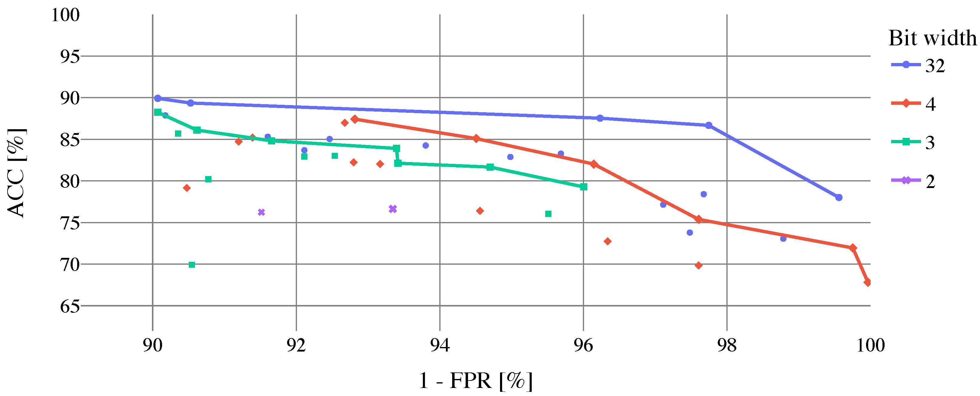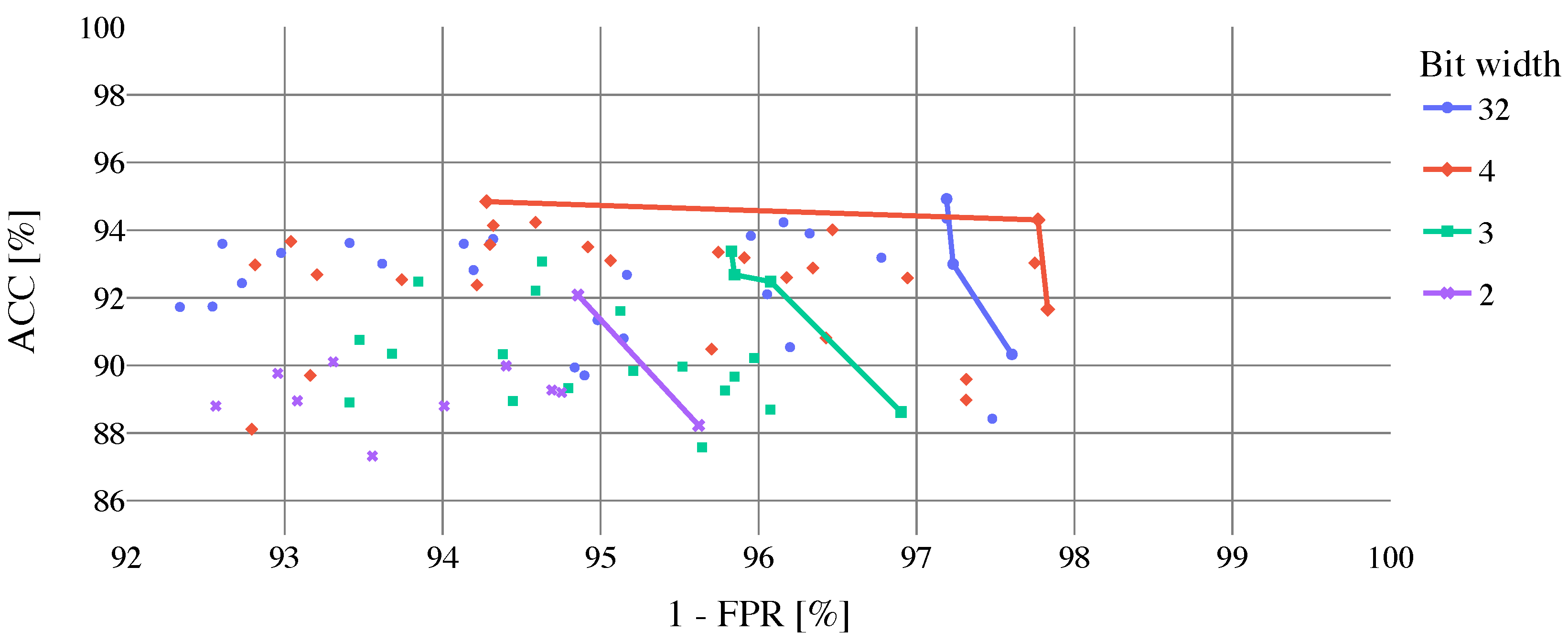$3\%$ of ACC. For more insights, the dependence of model ACC on FPR (with FPR value inverted for better readability) can be seen in Figure 9.

Optimal solutions, which represent a trade-off between ACC and FPR, are stressed out by Pareto fronts. Results of cloud coverage classification for best-performed 4-bit width models (4-bit width models are selected due to best accuracy/FPR ratio from quantized models) per biome using the full $\mathrm{L}8$ biome dataset are shown in

Table 5. Results of cloud coverage classification for best-performed 4-bit width models per biome employing full L8-D dataset.

Biome	ACC [%]	PRE [%]	REC [%]	F1 [%]	FPR [%]
Barren	87.32	85.69	83.83	84.75	10.14
Forest	84.01	99.29	68.36	80.97	0.49
SnowIce	69.24	50.47	70	58.65	31.11
GrassCrops	95.91	98.7	91.22	94.81	0.83
Shrubland	91.73	97.03	83.14	89.55	1.89
Urban	92.89	95.01	85.23	89.86	2.62
Water	93.89	94.32	90.82	92.54	3.92
Wetlands	84.41	98.51	68.33	80.69	0.94

ACC—accuracy; PRE—precision; REC—recall; F1—F1 score; FPR—false positive rate.

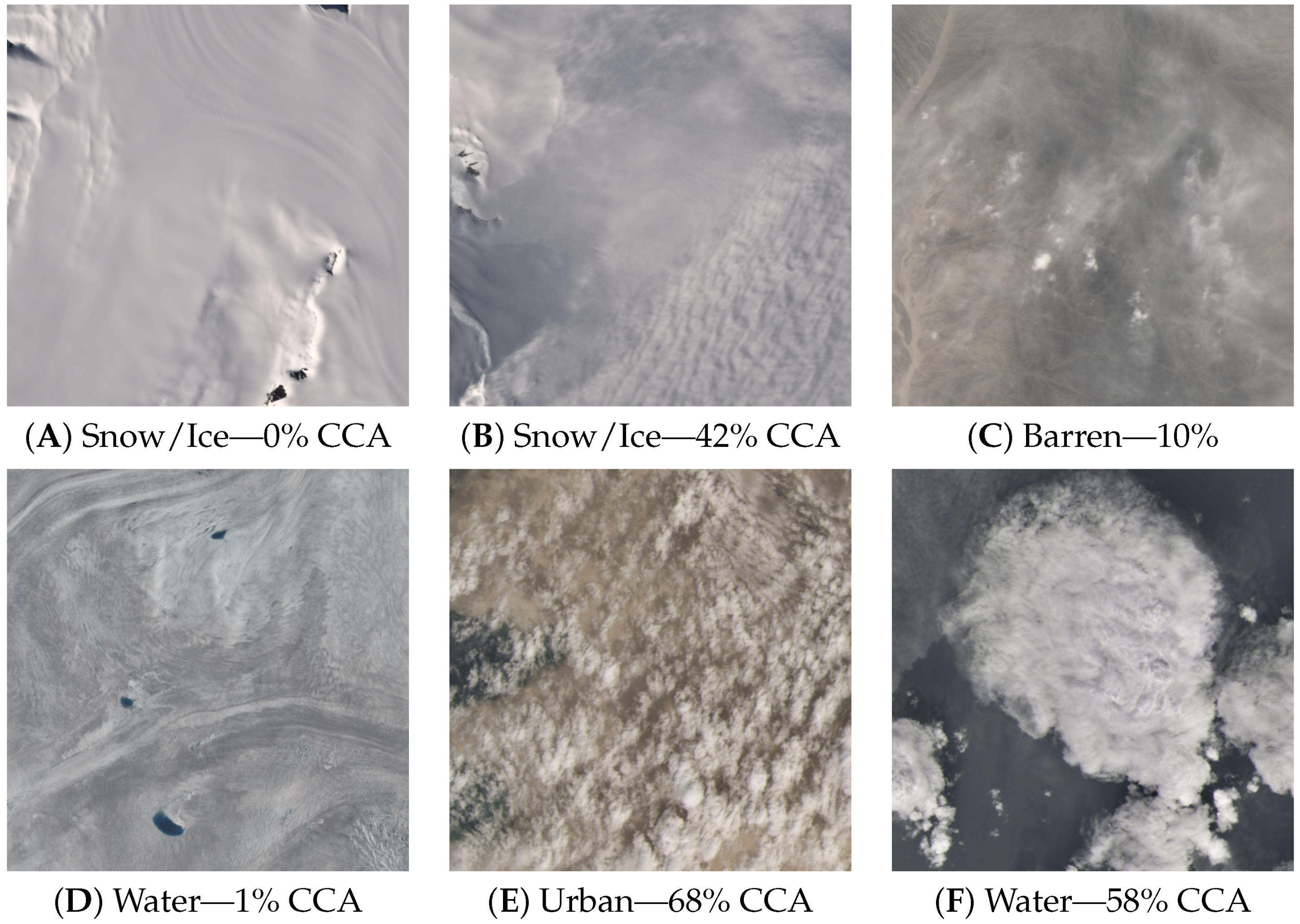
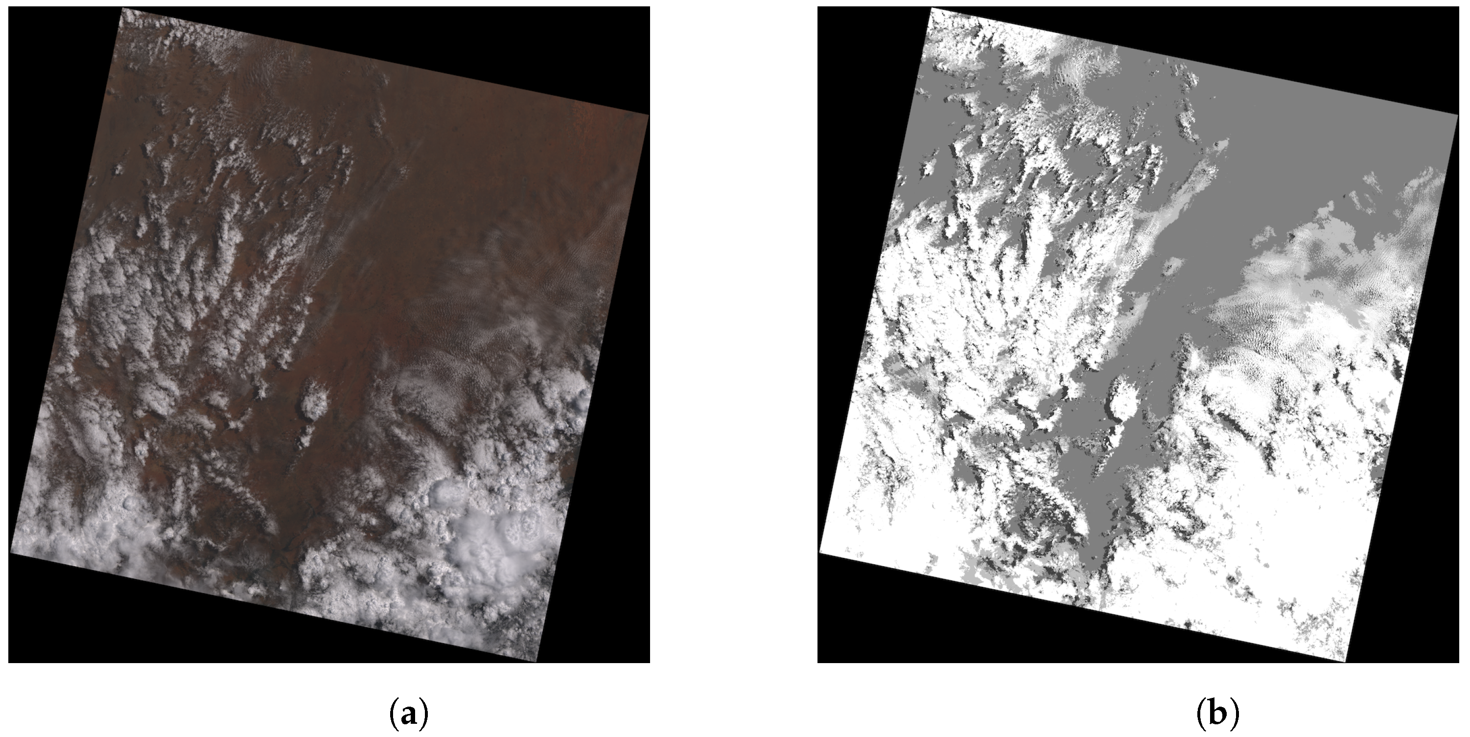
. Models are selected by the highest ACC. The model performed best on the Grass/Crops biome ($\mathrm{ACC}=95.91\%$ and $\mathrm{FPR}=0.83\%$). However the best $\mathrm{FPR}=0.49\%$ was achieved in the Forest biome, though with low $\mathrm{ACC}=84.01\%$. The worst performance ($\mathrm{ACC}=69.24\%$ and $\mathrm{FPR}=31.11\%$) was achieved on the Snow/Ice biome. Based on the results of the cloud coverage classification per biome, hypothesis is made that excluding the Snow/Ice biome (cloud coverage classification on Snow/Ice biome using natural color composite is irrelevant) from model training will improve overall model performance (especially FPR). For a better illustration of the problem, the examples of FP tiles are presented in Figure 10.

Results of cloud coverage classification using the $\mathrm{L}8$ biome dataset without Snow/Ice biome to train, validate and test the proposed CNN are shown in

Table 6. Results of cloud coverage classification for best-performed models using L8-D dataset excluding Snow/Ice biome.

Top Models by ACC
BW	ACC [%]	PRE [%]	REC [%]	F1 [%]	FPR [%]
32	94.92	96.12	91.93	93.98	2.81
4	94.84	92.68	95.58	94.11	5.72
3	93.37	94.24	90.13	92.14	4.17
2	92.08	92.87	88.41	90.59	5.14
Top Models by FPR
BW	ACC [%]	PRE [%]	REC [%]	F1 [%]	FPR [%]
32	94.92	96.12	91.93	93.98	2.81
4	94.30	96.82	89.72	93.14	2.23
3	92.48	94.42	87.73	90.96	3.92
2	92.08	92.87	88.41	90.59	5.14

BW—bit width; ACC—accuracy; PRE—precision; REC—recall; F1—F1 score; FPR—false positive rate. Top models by FPR are selected from top 10 models sorted by ACC.

. In the upper part of the table, best-performed models selected by ACC are presented. As can be noticed, in comparison with previous models trained by the full $\mathrm{L}8$ biome dataset the classification performance was improved ($\mathrm{ACC}\approx 92$–$95\%$, $\mathrm{FPR}\approx 2.9$–$5.7\%$). In the bottom part of Table 6, top models selected by FPR are shown (models are selected from the top 10 models sorted by ACC). In case of the 32 and 2-bit width models, there is no change in performance. However, FPR for 4 and 3-bit width models is lower, whereas 4-bit model outperforms the 32-bit width one. For a better illustration, the dependence of model ACC on FPR can be seen in Figure 11, where optimal solutions are highlighted by Pareto fronts.

Finally, the results of hardware architecture design space exploration are summarized. In

Table 7. FPGA resource utilization and performance for different model bit widths and folding setup.

BW	Folding	FPS	APC [W]	LUT [%]	FF [%]	BRAM [%]	DSP [%]
4	max	15.468	2.592	69.05	48.61	62.50	13.64
	SPEC	9.931	2.556	66.67	48.14	61.43	13.64
	base	0.879	2.484	58.42	46.96	57.14	0.45
3	max	15.467	2.556	58.90	40.39	47.86	13.64
	SPEC	9.932	2.520	58.30	40.01	46.79	13.64
	base	0.879	2.448	55.11	39.06	42.86	0.45
2	max	15.462	2.520	47.72	32.49	32.68	13.64
	SPEC	9.927	2.484	47.74	32.29	32.50	13.64
	base	0.879	2.448	46.27	31.41	29.29	0.45

BW—bit width; SPEC—targeting specifically 10 FPS; FPS—frames per second; APC—average power consumption; LUT—look up table utilization; FF—flip flop utilization; BRAM—block random memory utilization; DSP—digital signal processing slice utilization.

, the overview of resource utilization measurements of quantized models using different bit widths can be found. Maximum and base folding setup was compared together with folding setup targeting 10 FPS. Even though the FPS is changing from $0.9$ to $15.5$, the average power consumption is stable at around 2.5 W. The parallelization settings and their respective estimated number of clock cycles for targeting specifically 10 FPS are reported in

Table 8. Parallelization settings and their respective estimated number of clock cycles for targeting specific 10 FPS.

	Specific FPS Folding
Layer	(PE, SIMD)	Cycles
Conv_1	(10, 3)	2,359,296
Conv_2	(6, 10)	147,456
Conv_3	(3, 1)	1,769,472
Conv_4	(1, 2)	3,538,944
Conv_5	(1, 1)	442,368
Conv_6	(1, 1)	331,776
Conv_7	(1, 1)	442,368
Conv_8	(1, 1)	27,648
Conv_9	(1, 1)	20,736
Conv_10	(1, 2)	442,368
FC_1	(1, 2)	262,144
FC_2	(1, 1)	1024

PE—processing elements; SIMD—single instruction multiple data; Conv—convolution layer; FC—fully connected layer.

. Results of cloud coverage classification for best-performed quantized models on FPGA can be seen in

Table 9. Results of cloud coverage classification for best-performed quantized models on FPGA.

BW	ACC (SI) [%]	ACC (EXSI) [%]	FPS	RU [%]	APC [W]
2	83.41	92.08	15.462	31.63	2.520
3	88.24	93.37	15.467	40.20	2.556
4	87.42	94.84	15.468	48.45	2.592

BW—bit width; ACC—accuracy; SI—Snow/Ice biome included; EXSI—Snow/Ice biome excluded; FPS—frames per second; RU—FPGA resource utilization; APC—average power consumption.

. Classification ACC and FPGA resource utilization is reported for quantized models trained using the full $\mathrm{L}8$ biome dataset and dataset excluding the Snow/Ice biome from the dataset. The best-performed model is a quantized 4-bit width model with Snow/Ice biome excluded from training and evaluation ($\mathrm{ACC}=94.84\%$).

4. Discussion

4.1. Quantized Model for Cloud Detection

Based on the results of the best-performing models reported in the upper part of Table 4, the increase of the quantization level resulted in slight overall performance deterioration. Even though, the quantized models achieved comparable results to the 32-bit baseline model (except the 2-bit model). The decrease of the overall accuracy for the 4-bit and 3-bit model is just around $2\%$, while for the 2-bit model it is more than $6\%$. However, rather than the highest overall accuracy, this study emphasizes on the low FPR (it is more convenient to process a redundant image than to discard the relevant one). Therefore, a balance between the ACC and FPR is in demand. For the baseline model and 3-bit model, the FPR is identically equal to $9.93\%$. In the case of the 4-bit model, almost $3\%$ of FPR decrease can be noticed, however, the recall is lower by $10\%$ in comparison to the 32-bit model. The 2-bit model suffers the most from the quantization effect resulting in very insufficient $\mathrm{FPR}=17.59\%$. More balanced (ACC vs. FPR) results are provided in the bottom part of Table 4, where the best models by FPR from the top 10 models sorted by ACC are reported. Unfortunately, the performance of the quantized models keeps almost on the same levels, yet the baseline model significantly reduced its FPR to $2.25\%$, while decreasing its accuracy by around $3\%$. A more readable comparison of the model’s performance can be seen in Figure 9. A trend of the trade-off between ACC and FPR across all quantized models together with the baseline is highlighted by Pareto fronts. It can be observed, that the baseline model outperforms the quantized ones, however, there can be found adequate alternatives to the 32-bit model.

To collect more insights and to improve the overall performance of the proposed cloud detection system, each biome of the $\mathrm{L}8$ biome dataset was investigated separately. We hypothesize that some biomes produce significant noise during the training process due to the false cloud-like features (snow, ice, or fog). The 4-bit models were selected to investigate biomes in quantized cases, and its results are reported in Table 5. Best performance was obtained by a model trained on Grass/Crops biome with $\mathrm{ACC}=95.91\%$ and low $\mathrm{FPR}=0.83\%$. Yet, the best $\mathrm{FPR}=0.49\%$ and precision of more than $99\%$ was achieved by Forrest biome. However, this model lags on accuracy due to low $recall=68.36\%$, which will result in a high number of undetected cloudy images. This may be caused by the cloud categories merge (thin, thick) or by the fog, which is a usual false cloud-like feature in the Forest biome [34]. Similarly, the Wetlands biome (also often affected by fog) resulted in low $\mathrm{FPR}=0.94\%$ and high $\mathrm{precision}=98.51\%$, but with low $\mathrm{recall}=68.33\%$. The Shrubland, Urban, and Water biomes achieved comparable performance with ACC from $91.73\%$ to $93.89\%$ and FPR from $1.89\%$ to $3.92\%$. The Barren biome obtained the second worse performance in terms of $\mathrm{FPR}=10.14\%$. The reason for high FPR may lie in the nature of the Barren biome, which exaggerates the thin clouds features to thick clouds. The worst performance reports the Snow/Ice biome. Low precision of $50.47\%$ and high $\mathrm{FPR}=31.11\%$ make its decision almost random. Since only the RGB channels were considered, the reason for misclassification is the inability to recognize between cloud, ice, and snow. To be able to classify the clouds above the snow and ice, an additional spectrum capable of altitude resolution will be necessary [6,10,34].

Regarding the previously mentioned results, all biomes, to a certain degree, suffer from the cloud-like features problem. An example is given in Figure 10, where six misclassified cases are presented. The first example of the Snow/Ice biome (A) has $\mathrm{CCA}=0\%$, yet the snow in the image was misclassified to a cloud. The second example of Snow/Ice biome (B) with $\mathrm{CCA}=42\%$ merged cloud with turbid snow currents. Next, the smooth hilly terrain of the Barren biome (C) stretches the features of thinly dispersed clouds. This resulted in the falsely positive image, however, the CCA is $10\%$ in reality. Similarly, the Water biome example (D) with $\mathrm{CCA}=1\%$ was misclassified due to the wavy, serpentine features of the shallow water. The last two examples (E, F) in Figure 10 represent the case near the threshold ($\mathrm{CCA}=70\%$). Hereabouts, a small number of cloud pixels may flip the CCA over the threshold boundary. In addition, the precise value of the CCA for each tile may be softly different from the CCA label [35,37].

Following the reported results, the Snow/Ice biome is not suitable for the cloud detection using the proposed method. Moreover, problematic coexistence of the snow, ice and cloud in cloud detection systems has been also identified by [6,10,34]. Therefore, we decided to withdraw the Snow/Ice biome from the train, validation and test datasets, and to perform the experiment without this noisy data. In the real use case, the cloud detection system can omit known areas permanently covered by snow or ice from the analysis. Based on the results reported in Table 6, assumed improvements of all metrics can be observed. The best performing baseline model achieved $\mathrm{ACC}=94.92\%$ with $\mathrm{FPR}=2.81\%$. Top quantized models obtained comparable accuracy from $94.84\%$ to $92.02\%$, and FPR from $2.23\%$ to $5.72\%$. We would like to stress out, that 4-bit quantized model performed slightly better in terms of precision ($96.82\%$) and FPR ($2.23\%$) in comparison to the 32-bit model. This makes it a proper quantized substitution for deployment on FPGA. Results of this analysis confirm our hypothesis that Snow/Ice biome is naturally prone to being false positive when using RGB channels only.

In Figure 11, the accuracy vs. FPR is visualized for models trained with excluded Snow/Ice biome. From elevated position of all models within this Figure it is evident that accuracy increased all-around in comparison to Figure 9. Curves of Pareto fronts lie closer together and to the baseline front, as the quantization takes a lower toll on models performance when without visually ambiguous data.

Based on these results, following observations will be emphasised to make a deduction. Increased quantization did not cause substantial drop in values for evaluation metrics scores of results with excluded Snow/ice biome. The 4-bit model matched or overtook baseline’s metric scores in accuracy and FPR. This implies equality between representational capacity of 32-bit baseline and quantized models in classifier problems that do not require high resolution for discerning discriminative features. This statement is in line with results achieved in other works [46,55,56] dealing with the quantization.

The most relevant study, CloudScout [20,34], used hyperspectral bands for model training, resulting to 16-bit model with $\mathrm{ACC}=92\%$ and $\mathrm{FPR}=1\%$. Our proposed method outperformed this result by a 4-bit model with higher accuracy up to $3\%$, however with lower FPR by $1.23\%$. Considering, that our model used RGB bands only (without Snow/Ice biome), the presented CloudSatNet-1 method brings promising improvements in the on-board cloud detection systems. Another relevant study [21] used a larger training dataset and achieved ACC of $91\%$. Nevertheless, when authors deployed the model on FPGA, a significant drop of accuracy to $64\%$ occurred. The method introduced in this paper does not encounter a similar issue. The comparison of these methods is summarized in

Table 10. Comparison of the best-performed models with different studies.

Method	BW	ACC [%]	FPR [%]	APC [W]	Data
CloudSatNet-1 *	4	94.84	2.23	2.5	RGB
CloudScout [20]	16	92	1	1.8	Hyperspectral
CNV-W1A1 [21]	1	64	-	2.4	RGB

*—proposed method; BW—bit width; ACC—accuracy; FPR—false positive rate; APC—average power consumption.

.

4.2. FPGA-Based Hardware Accelerator

The quantized models were deployed in three folding configurations for each bit width setting. Throughput, power consumption, and FPGA resource utilization were measured. Models with maximum folding achieved 15 FPS with input batch size of 1 and almost 20 FPS with batch size 120 which is the maximal batch size allowed to be loaded into RAM. Increase of the FPS with higher batch size was expected, and also confirmed by [3]. Power consumption measured with a USB power meter reported an increase of just over ≈$0.2 \mathrm{W}$ during the inference, compared to the resting state. In comparison with related studies, the authors of CloudScout [20,34] reported a throughput of 2.89 FPS and 1.8 W of power consumption using Myriad VPU with 512 × 512 × 3 input size, 7 FPS and 3.4 W of power consumption using Zynq Ultrascale+ ZCU106, and 3.77 FPS using XQRKU060 solution (estimation only). Next, in the study by Reiter et al. [21], the authors reported 358.1 FPS with a much smaller input size 32 × 32 × 3, and maximum power consumption of 2.4 W. Regarding these results, the throughput and power consumption of the hardware accelerator achieved in this study is comparable with the current state-of-the-art solutions.

Based on the estimated number of cycles per layer reported in Table 3, it is visible that a bottle-neck in the first layer limited the optimal throughput, and it would require a change in the network architecture to allow a higher throughput target. It was demonstrated that the network throughput can be controlled to target a specific FPS desired by the needs of the mission. A set of experiments were conducted to target specific throughput of 10 FPS. Used parallelization settings are reported in Table 8. This approach may be useful when the instrument on the CubeSat does not have a high throughput, e.g., the camera is generating data at lower FPS. It showed flexibility in throughput control of the FPGA-based hardware accelerator created by the FINN framework. The differences for each bit width are in FPGA resource utilization, where the 2-bit model in base folding configuration utilized the lowest number of the resources ($\mathrm{LUT}=46.27\%$, $\mathrm{FF}=31.41\%$, $\mathrm{BRAM}=29.29\%$, $\mathrm{DSP}=0.45\%$). This is achieved due to no parallelization and a low memory footprint of 2-bit weights and activations. It shows the potential to reduce bit width for weights and activations even further to 1-bit and experiment with BNN in the future to enable higher throughput and deeper network on the same FPGA. As presented in Table 7, DSP slices for the first layer were selected to be utilized by Vivado just for SPEC and max folding in all bit width configurations. Memory footprint (BRAM utilization) varies from 1.43 Mb to 3.06 Mb in the ascending order relative to bit width.

5. Conclusions

Most of the RSI is contaminated by the clouds, hence the quick and accurate method of cloud removal running on-board of the satellite has potential to significantly save the downlink. In this study, we introduced CloudSatNet-1, an FPGA-based hardware-accelerated quantized CNN for satellite on-board cloud coverage classification. We can conclude that the weights and activations quantization has a minimal or no effect on the model accuracy. However, the memory footprint reduction allows the model deployment and testing on low-cost FPGA Xilinx Zynq-7020. Using the $\mathrm{L}8$ biome dataset and its RGB bands only, up to $90\%$ of accuracy was achieved. Next, we omitted the Snow/Ice biome tiles from the dataset due to high noise production. The accuracy increased up to $94.4\%$ of accuracy with low $FPR=2.23\%$ for the 4-bit width model. With the maximum parallelization settings, the hardware accelerator achieved 15 FPS with 2.5 W of average power consumption (0.2 W increase over the idle state). Additionally, we proved that we can control throughput to target specific FPS for the proposed classifier. Considering the reported results, the presented novel approach achieved outcome comparable with the state of the art.

The presented solution has several limitations that we would like to stress out. Firstly, the high number of false positive tiles with a terrain containing cloud-like features may be in the future compensated with the analysis involving the multi-spectral bands. Next, the cloud categories from the original $\mathrm{L}8$ biome dataset were merged to form a binary problem. Therefore, this study did not evaluate the result on the original cloud categories of the $\mathrm{L}8$ biome dataset, which might provide more insights on miss-classifications. Furthermore, we did not cover the effects of the radiation on the cloud detection system and the redundancy will be subject of the future works. This work is the beginning of the greater effort to provide solutions based on AI for the space missions that can benefit from it, thus this work is a pilot one in nature. In the future, we aim to improve this solution to provide semantic segmentation of clouds with clouds categorization to respective classes compensating for the binary decision provided in this study.

References

1. Lofqvist, M.; Cano, J. Optimizing Data Processing in Space for Object Detection in Satellite Imagery. arXiv 2021, arXiv:2107.03774. [Google Scholar]
2. Caldwell, S. State-of-the-Art of Small Spacecraft Technology; NASA: Washington, DC, USA, 2021.
3. Maskey, A.; Cho, M. CubeSatNet: Ultralight Convolutional Neural Network designed for on-orbit binary image classification on a 1U CubeSat. Eng. Appl. Artif. Intell. 2020, 96, 103952. [Google Scholar] [CrossRef]
4. Kulu, E. Nanosats Database. 2022. Available online: https://www.nanosats.eu/ (accessed on 15 September 2021).
5. EUSPA. EUSPA EO and GNSS Market Report; EUSPA: Prague, Czech Republic, 2022. [Google Scholar]
6. Yang, J.; Guo, J.; Yue, H.; Liu, Z.; Hu, H.; Li, K. CDnet: CNN-based cloud detection for remote sensing imagery. IEEE Trans. Geosci. Remote Sens. 2019, 57, 6195–6211. [Google Scholar] [CrossRef]
7. Fenta, A.A.; Yasuda, H.; Haregeweyn, N.; Belay, A.S.; Hadush, Z.; Gebremedhin, M.A.; Mekonnen, G. The dynamics of urban expansion and land use/land cover changes using remote sensing and spatial metrics: The case of Mekelle City of northern Ethiopia. Int. J. Remote Sens. 2017, 38, 4107–4129. [Google Scholar] [CrossRef]
8. King, M.D.; Platnick, S.; Menzel, W.P.; Ackerman, S.A.; Hubanks, P.A. Spatial and temporal distribution of clouds observed by MODIS onboard the Terra and Aqua satellites. IEEE Trans. Geosci. Remote Sens. 2013, 51, 3826–3852. [Google Scholar] [CrossRef]
9. Zhang, Y.; Rossow, W.B.; Lacis, A.A.; Oinas, V.; Mishchenko, M.I. Calculation of radiative fluxes from the surface to top of atmosphere based on ISCCP and other global data sets: Refinements of the radiative transfer model and the input data. J. Geophys. Res. Atmos. 2004, 109, D19105. [Google Scholar] [CrossRef] [Green Version]
10. Guo, J.; Yang, J.; Yue, H.; Tan, H.; Hou, C.; Li, K. CDnetV2: CNN-based cloud detection for remote sensing imagery with cloud-snow coexistence. IEEE Trans. Geosci. Remote Sens. 2020, 59, 700–713. [Google Scholar] [CrossRef]
11. Wu, Z.; Li, J.; Wang, Y.; Hu, Z.; Molinier, M. Self-attentive generative adversarial network for cloud detection in high resolution remote sensing images. IEEE Geosci. Remote Sens. Lett. 2019, 17, 1792–1796. [Google Scholar] [CrossRef]
12. Li, L.; Li, X.; Jiang, L.; Su, X.; Chen, F. A review on deep learning techniques for cloud detection methodologies and challenges. Signal Image Video Process. 2021, 15, 1527–1535. [Google Scholar] [CrossRef]
13. Kreuter, A.; Zangerl, M.; Schwarzmann, M.; Blumthaler, M. All-sky imaging: A simple, versatile system for atmospheric research. Appl. Opt. 2009, 48, 1091–1097. [Google Scholar] [CrossRef]
14. Long, C.N.; Sabburg, J.M.; Calbó, J.; Pagès, D. Retrieving cloud characteristics from ground-based daytime color all-sky images. J. Atmos. Ocean. Technol. 2006, 23, 633–652. [Google Scholar] [CrossRef] [Green Version]
15. Frantz, D.; Haß, E.; Uhl, A.; Stoffels, J.; Hill, J. Improvement of the Fmask algorithm for Sentinel-2 images: Separating clouds from bright surfaces based on parallax effects. Remote Sens. Environ. 2018, 215, 471–481. [Google Scholar] [CrossRef]
16. Zhu, Z.; Woodcock, C.E. Automated cloud, cloud shadow, and snow detection in multitemporal Landsat data: An algorithm designed specifically for monitoring land cover change. Remote Sens. Environ. 2014, 152, 217–234. [Google Scholar] [CrossRef]
17. Sui, Y.; He, B.; Fu, T. Energy-based cloud detection in multispectral images based on the SVM technique. Int. J. Remote Sens. 2019, 40, 5530–5543. [Google Scholar] [CrossRef]
18. Zi, Y.; Xie, F.; Jiang, Z. A cloud detection method for Landsat 8 images based on PCANet. Remote Sens. 2018, 10, 877. [Google Scholar] [CrossRef] [Green Version]
19. Miralles, P.; Scannapieco, A.F.; Jagadam, N.; Baranwal, P.; Faldu, B.; Abhang, R.; Bhatia, S.; Bonnart, S.; Bhatnagar, I.; Batul, B.; et al. Machine Learning in Earth Observation Operations: A review. In Proceedings of the 72nd International Astronautical Congress (IAC), Dubai, United Arab Emirates, 25–29 October 2021; International Astronautical Federation: Paris, France, 2021. [Google Scholar]
20. Rapuano, E.; Meoni, G.; Pacini, T.; Dinelli, G.; Furano, G.; Giuffrida, G.; Fanucci, L. An FPGA-Based Hardware Accelerator for CNNs Inference on Board Satellites: Benchmarking with Myriad 2-Based Solution for the CloudScout Case Study. Remote Sens. 2021, 13, 1518. [Google Scholar] [CrossRef]
21. Reiter, P.; Karagiannakis, P.; Ireland, M.; Greenland, S.; Crockett, L. FPGA acceleration of a quantized neural network for remote-sensed cloud detection. In Proceedings of the 7th International Workshop on On-Board Payload Data Compression, Online, 21–23 September 2020. [Google Scholar]
22. Vloncar. fastmachinelearning/hls4ml: Coris; Zenodo: Geneva, Switzerland, 2021. [Google Scholar] [CrossRef]
23. Blott, M.; Preußer, T.B.; Fraser, N.J.; Gambardella, G.; O’brien, K.; Umuroglu, Y.; Leeser, M.; Vissers, K. FINN-R: An end-to-end deep-learning framework for fast exploration of quantized neural networks. ACM Trans. Reconfig. Technol. Syst. TRETS 2018, 11, 1–23. [Google Scholar] [CrossRef]
24. Yao, Y.; Jiang, Z.; Zhang, H.; Zhou, Y. On-board ship detection in micro-nano satellite based on deep learning and COTS component. Remote Sens. 2019, 11, 762. [Google Scholar] [CrossRef] [Green Version]
25. Schwartz, C.; Sander, I.; Jordão, R.; Bruhn, F.; Persson, M.; Ekblad, J.; Fuglesang, C. On-board satellite data processing to achieve smart information collection. In Optics, Photonics and Digital Technologies for Imaging Applications VII; Schelkens, P., Kozacki, T., Eds.; International Society for Optics and Photonics, SPIE: Bellingham, WA, USA, 2022; Volume 12138, pp. 121–131. [Google Scholar] [CrossRef]
26. ElMasry, G.; Sun, D.W. Principles of Hyperspectral Imaging Technology. In Hyperspectral Imaging for Food Quality Analysis and Control; Elsevier: Amsterdam, The Netherlands, 2010; pp. 3–43. [Google Scholar]
27. Zhang, Z.; Iwasaki, A.; Xu, G.; Song, J. Cloud detection on small satellites based on lightweight U-net and image compression. J. Appl. Remote Sens. 2019, 13, 026502. [Google Scholar] [CrossRef]
28. Zhang, J.; Li, X.; Li, L.; Sun, P.; Su, X.; Hu, T.; Chen, F. Lightweight U-Net for cloud detection of visible and thermal infrared remote sensing images. Opt. Quantum Electron. 2020, 52, 1–14. [Google Scholar] [CrossRef]
29. Zhang, Z.; Xu, G.; Song, J. CubeSat cloud detection based on JPEG2000 compression and deep learning. Adv. Mech. Eng. 2018, 10, 1687814018808178. [Google Scholar] [CrossRef] [Green Version]
30. Park, J.H.; Inamori, T.; Hamaguchi, R.; Otsuki, K.; Kim, J.E.; Yamaoka, K. RGB Image Prioritization Using Convolutional Neural Network on a Microprocessor for Nanosatellites. Remote Sens. 2020, 12, 3941. [Google Scholar] [CrossRef]
31. Greenland, S.; Ireland, M.; Kobayashi, C.; Mendham, P.; Post, M.; White, D. Development of a minaturised forwards looking imager using deep learning for responsive operations. In Proceedings of the 4S Symposium, Sorrento, Italy, 28 May–1 June 2018; ESA: Paris, France, 2018. [Google Scholar]
32. de Vieilleville, F.; Lagrange, A.; Ruiloba, R.; May, S. Towards Distillation of Deep Neural Networks for Satellite On-Board Image Segmentation. Int. Arch. Photogramm. Remote Sens. Spat. Inf. Sci. 2020, 43, 1553–1559. [Google Scholar] [CrossRef]
33. Li, J.; Wu, Z.; Hu, Z.; Jian, C.; Luo, S.; Mou, L.; Zhu, X.X.; Molinier, M. A Lightweight Deep Learning-Based Cloud Detection Method for Sentinel-2A Imagery Fusing Multiscale Spectral and Spatial Features. IEEE Trans. Geosci. Remote Sens. 2021, 60, 1–19. [Google Scholar] [CrossRef]
34. Giuffrida, G.; Diana, L.; de Gioia, F.; Benelli, G.; Meoni, G.; Donati, M.; Fanucci, L. Cloudscout: A deep neural network for on-board cloud detection on hyperspectral images. Remote Sens. 2020, 12, 2205. [Google Scholar] [CrossRef]
35. Foga, S.; Scaramuzza, P.L.; Guo, S.; Zhu, Z.; Dilley Jr, R.D.; Beckmann, T.; Schmidt, G.L.; Dwyer, J.L.; Hughes, M.J.; Laue, B. Cloud detection algorithm comparison and validation for operational Landsat data products. Remote Sens. Environ. 2017, 194, 379–390. [Google Scholar] [CrossRef] [Green Version]
36. Markham, B.; Storey, J.; Morfitt, R. Landsat-8 sensor characterization and calibration. Remote Sens. 2015, 7, 2279–2282. [Google Scholar] [CrossRef] [Green Version]
37. USGS. Landsat Data Continuity Mission Level 1 (L1) Data Format Control Book (DFCB), LDCM-DFCB-004, Version 6.0; USGS: Reston, VA, USA, 2012.
38. Loveland, T.R.; Reed, B.C.; Brown, J.F.; Ohlen, D.O.; Zhu, Z.; Yang, L.; Merchant, J.W. Development of a global land cover characteristics database and IGBP DISCover from 1 km AVHRR data. Int. J. Remote Sens. 2000, 21, 1303–1330. [Google Scholar] [CrossRef]
39. Gholami, A.; Kim, S.; Dong, Z.; Yao, Z.; Mahoney, M.W.; Keutzer, K. A Survey of Quantization Methods for Efficient Neural Network Inference. arXiv 2021, arXiv:2103.13630. [Google Scholar]
40. Pappalardo, A. Xilinx/brevitas; Zenodo: Geneva, Switzerland, 2021. [Google Scholar] [CrossRef]
41. Quantization. Available online: https://pytorch.org/docs/stable/quantization.html (accessed on 28 November 2021).
42. Courbariaux, M.; Hubara, I.; Soudry, D.; El-Yaniv, R.; Bengio, Y. Binarized neural networks: Training deep neural networks with weights and activations constrained to+ 1 or-1. arXiv 2016, arXiv:1602.02830. [Google Scholar]
43. Alonso, T.; Petrica, L.; Ruiz, M.; Petri-Koenig, J.; Umuroglu, Y.; Stamelos, I.; Koromilas, E.; Blott, M.; Vissers, K. Elastic-DF: Scaling Performance of DNN Inference in FPGA Clouds through Automatic Partitioning. ACM Trans. Reconfigurable Technol. Syst. 2021, 15, 1–34. [Google Scholar] [CrossRef]
44. Przewlocka, D.; Wasala, M.; Szolc, H.; Blachut, K.; Kryjak, T. Optimisation of a Siamese Neural Network for Real-Time Energy Efficient Object Tracking. arXiv 2020, arXiv:2007.00491. [Google Scholar]
45. Mellempudi, N.; Kundu, A.; Mudigere, D.; Das, D.; Kaul, B.; Dubey, P. Ternary Neural Networks with Fine-Grained Quantization. arXiv 2017, arXiv:1705.01462. [Google Scholar]
46. Zhou, S.; Wu, Y.; Ni, Z.; Zhou, X.; Wen, H.; Zou, Y. DoReFa-Net: Training Low Bitwidth Convolutional Neural Networks with Low Bitwidth Gradients. arXiv 2016, arXiv:1606.06160. [Google Scholar]
47. Ioffe, S.; Szegedy, C. Batch Normalization: Accelerating Deep Network Training by Reducing Internal Covariate Shift. Proc. Mach. Learn. Res. PMLR 2015, 37, 448–456. [Google Scholar]
48. Umuroglu, Y.; Jahre, M. Streamlined Deployment for Quantized Neural Networks. arXiv 2017, arXiv:1709.04060. [Google Scholar]
49. Crockett, L.; Northcote, D.; Ramsay, C. Exploring Zynq MPSoC: With PYNQ and Machine Learning Applications; Strathclyde Academic Media: Glasgow, Scotland, 2019. [Google Scholar]
50. Xilinx. Zynq-7000 SoC Data Sheet: Overview. 2018. Available online: https://www.xilinx.com/content/dam/xilinx/support/documents/data_sheets/ds190-Zynq-7000-Overview.pdf (accessed on 8 September 2021).
51. PYNQ: PYTHON PRODUCTIVITY. Available online: http://www.pynq.io/ (accessed on 8 February 2022).
52. Developers, O.R. ONNX Runtime. Version: X.y.z. 2021. Available online: https://onnxruntime.ai/ (accessed on 1 September 2021).
53. Shahriari, B.; Swersky, K.; Wang, Z.; Adams, R.P.; de Freitas, N. Taking the Human Out of the Loop: A Review of Bayesian Optimization. Proc. IEEE 2016, 104, 148–175. [Google Scholar] [CrossRef] [Green Version]
54. Faraone, J.; Gambardella, G.; Boland, D.; Fraser, N.; Blott, M.; Leong, P.H. Customizing Low-Precision Deep Neural Networks for FPGAs. In Proceedings of the 2018 28th International Conference on Field Programmable Logic and Applications (FPL), Dublin, Ireland, 26–30 August 2018; pp. 97–973. [Google Scholar] [CrossRef]
55. Han, S.; Mao, H.; Dally, W.J. Deep compression: Compressing deep neural networks with pruning, trained quantization and huffman coding. arXiv 2015, arXiv:1510.00149. [Google Scholar]
56. Zhu, C.; Han, S.; Mao, H.; Dally, W.J. Trained ternary quantization. arXiv 2016, arXiv:1612.01064. [Google Scholar]
Figure 1. L 8 Biome dataset image patch example (a) reconstructed from bands B4, B3, and B2 with its associated multi-class cloud mask (b) [35]. (a) Image patch. (b) Cloud validation mask.
Remotesensing 14 03180 g001
Figure 2. Distribution of the L 8 biome dataset scenes CCA values [35].
Remotesensing 14 03180 g002
Figure 3. Image patches examples for each biome in the L 8 biome dataset [35]. (a) Barren. (b) Forest. (c) Grass/Crops. (d) Shrubland. (e) Snow/Ice. (f) Urban. (g) Water. (h) Wetlands.
Remotesensing 14 03180 g003
Figure 4. L 8 Biome dataset scene during different preprocessing steps [35]. (a) Image patch. (b) Rotated patch. (c) Cropped patch with tiling.
Remotesensing 14 03180 g004
Figure 5. Distribution of the tiles and its CCA values per biome for the full L 8 biome dataset. Tiles with CCA 70 % are categorized as cloudy and the rest are categorized as not cloudy tiles.
Remotesensing 14 03180 g005
Figure 6. Distribution of the tiles and its CCA values per biome for the training, validation and testing dataset.
Remotesensing 14 03180 g006
Figure 7. CloudSatNet-1 architecture.
Remotesensing 14 03180 g007
Figure 8. Scheme of proposed workflow.
Remotesensing 14 03180 g008
Figure 9. Dependence of model ACC on inverse FPR value ( 100 % 0 % FPR) using full L8-D dataset. Optimal solutions are highlighted by Pareto fronts.
Remotesensing 14 03180 g009
Figure 10. False positive tile examples: (A,B) represent the Snow/Ice biome; (C,D) represent cloud-like FP tiles; (E,F) represent FP tile close to threshold ( 70 % ).
Remotesensing 14 03180 g010
Figure 11. Dependence of model ACC on inverse FPR value ( 100 % 0 % FPR) using L8-D dataset excluding Snow/Ice biome. Optimal solutions are highlighted by Pareto fronts.
Remotesensing 14 03180 g011