Rice Height Monitoring between Different Estimation Models Using UAV Photogrammetry and Multispectral Technology

Abstract

Unmanned aerial vehicle (UAV) photogrammetry was used to monitor crop height in a flooded paddy field. Three multi-rotor UAVs were utilized to conduct flight missions in order to capture RGB (RedGreenBlue) and multispectral images, and these images were analyzed using several different models to provide the best results. Two image sets taken by two UAVs, mounted with RGB cameras of the same resolution and Global Navigation Satellite System (GNSS) receivers of different accuracies, were applied to perform photogrammetry. Two methods were then proposed for creating crop height models (CHMs), one of which was denoted as the M1 method and was based on the Digital Surface Point Cloud (DSPC) and the Digital Terrain Point Cloud (DSPT). The other was denoted as the M2 method and was based on the DSPC and a bathymetric sensor. An image set taken by another UAV mounted with a multispectral camera was used for multispectral-based photogrammetry. A Normal Differential Vegetation Index (NDVI) and a Vegetation Fraction (VF) were then extracted. A new method based on multiple linear regression (MLR) combining the NDVI, the VF, and a Soil Plant Analysis Development (SPAD) value for estimating the measured height (MH) of rice was then proposed and denoted as the M3 method. The results show that the M1 method, the UAV with a GNSS receiver with a higher accuracy, obtained more reliable estimations, while the M2 method, the UAV with a GNSS receiver of moderate accuracy, was actually slightly better. The effect on the performance of CHMs created by the M1 and M2 methods is more negligible in different plots with different treatments; however, remarkably, the more uniform the distribution of vegetation over the water surface, the better the performance. The M3 method, which was created using only a SPAD value and a canopy NDVI value, showed the highest coefficient of determination (${\mathrm{R}}^2$) for overall MH estimation, 0.838, compared with other combinations.

1. Introduction

Rice is one of the staple foods of many countries and regions, so an adequate rice supply is essential [1,2]. Improvements in field management and crop monitoring is one strategy used to meet crop production demand [3]. The field-based phenotype (FBP) is one of the essential components of a crop system, as it is the eventual expression of the crop’s genetic factors [4], which are crucial to improve crop production [5]. FBPs are various, including some morphological traits, for example, crop height (CH), lodging, crop canopy cover (CCC), and physiological traits such as leaf chlorophyll content (LCC) and biomass. Leaf chlorophyll content is one of the essential indicators used to evaluate the growth status of crops and can be used to understand a crop’s environmental stress and the level of N content [6,7]. Crop canopy cover is another important FBP that can indicate a crop’s emergence or the senescence status of certain crops [8]. Crop height is an important indicator, and a fundamental phenotypic parameter of crops; [9] has shown the correlation between CH and wheat biomass. Measuring these traits is therfore essential and significant in terms of crop yield improvements. In order to obtain data for FBPs, field-based crop-monitoring during the growing season is necessary. The specifics of crop-monitoring are based on the object of study and its detection items. For instance, [10] is related to the above-ground biomass monitoring of maize, whereas [11] concerns rice Leaf Area Index (LAI) monitoring. To perform crop-monitoring, crop growth surveys (CGSs) are indispensable. In the past, CGSs have usually been performed manually using traditional measurement methods such as a steel straight ruler for measuring crop height or other handheld instruments for collecting crop growth indication data. However, this is not only time-consuming and labor-intensive work, especially when crop areas are large [12], but it is also dangerous and uneconomical in inaccessible areas [13]. In recent years, research has considered many automated and semi-automated crop survey tools and these have been gradually introduced into precision agriculture CGSs [14].

UAV-based measurements are one of the progressive technologies that have been introduced into agriculture in the past decade [15]. The use of UAVs with onboard cameras, with which it is possible to effectively access field information and apply this to different cropping systems, has been extensively discussed in precision agriculture [16]. In agriculture applications, proximal UAV technology can capture the fields from the air with a relatively higher resolution and wider area of assessment when compared to remote satellites and ground wheeled vehicles [17,18,19]. The technique of UAV-based phenotyping may be an effective approach when collecting FBPs due to the fact that it is not only rapid but it is also non-invasive and non-disruptive. UAV photogrammetry and multispectral high-throughput analysis are two ways to perform phenotype processing [20,21]. By taking crop images on-site, environment optics information and various spatial information (e.g., shape, position, etc.) can be implicitly or explicitly measured, and then the extracted results can be studied to find the association between physiological indicators and the physical traits of crops. Not only can UAV-based CGSs reduce time and economic costs and, to some extent, increase efficiency, they can also yield more results and do this faster [22]. Moreover, a UAV-based crop survey can yield non-contact results, whereas human activities within the crop must, by necessity, cause some disruption and damage. UAV-based computer image technology can be used to collect phenotypic data, and the RGB and multispectral cameras mounted on a UAV can simultaneously capture shape information and spectra from continuous multi-temporal images [23].

Before performing UAV digital photogrammetry, ground control points (GCPs) need to be deployed in advance for the purpose of guided image matching [24]. Due to Global Navigation Satellite System (GNSS) technologys being increasingly used for recording camera shot locations, UAV-based digital photogrammetry based on GNSSs and GCPs have been used in many crop-monitoring as well as phenotypic studies [16,22]. In recent years, with further developments of GNSS technologies, UAVs using positioning techniques based on Real Time Kinematic (RTK) positioning, which measures the signal carrier wave phase in addition to the signal itself and then relies on a mobile station or virtual network station to provide real-time corrections, have been developed and widely discussed [25]. Compared with more commonly used Deferential Global Position System (DGPS) technology, RTK-based positioning can provide up to centimeter-level accuracy. With the reduction of positioning errors, computer vision technology allows for better matching of features in order to improve accuracy, which provides the possibility of moving away from deploying traditional GCPs [26,27]. In the absence of or inability to deploy GCPs, the positioning information of GNSSs onboard UAVs may be a potential factor in ensuring the comparability of photogrammetry results on different dates and has been widely discussed in recent years [28,29].

Vegetation index is an outcome of spectral analysis, which is a transformation of two or more spectral bands and was designed to qualitatively and quantitatively evaluate vegetation characteristics [30]. The spectral response of different vegetated fields are diverse, implying a complex mixture of the vegetation itself, soil brightness, environmental effects, shadow, soil color, and moisture [30]. The Normalized Difference Vegetation Index (NDVI) is one of the vegetation indices calculated by the reflectance of RED and NIR bands, which can be used in crop studies as an indicator of vegetation variations [31]. The NDVI of leaves changes continuously throughout the growth period of the crop, which means that NDVI-based data can be used to reflect the crop growth during different periods [32]. A NDVI of the crop canopy is often used as one of the predictors of crop yield and height, etc [33].

Measured height (MH) is a common data for assessing CH. The UAV-based CHM usually represents the difference between a digital surface model (DSM), which represents the surface of vegetation acquired by UAV-based measurement techniques, and its corresponding digital terrain model (DTM) or digital elevation model (DEM), which represents the terrain [34,35]. UAV-based photogrammetry often cannot fully and correctly capture the complete information of the crop canopy in a cropping system and its growing surface layer [36]. So, the results of created CHM data are not equivalent to the MH data of rice. Moreover, most previous studies on the relationship between CHM and MH data based on UAV measurement technologies have focused on crops growing in non-irrigated fields, such as wheat [34], maize [37], ryegrass [38], and upland rice [39], which all share the distinct feature that the growing ground surface layer of the crop is visible to the UAV. During the growing period of rice, the paddy field needs to be flooded so that the surface of the plow layer where the growing point of rice is located is invisible to the UAV. Malambo et al. [36] and Jimenez-Berni et al. [40] used a non-cropped field measured by a UAV-based measurement technique as a normalized reference for the field in other periods. However, this was still done in upland fields, and uniformly fixed markers were deployed throughout the experiment to ensure the stability of the photogrammetry over different dates. In irrigated and flooded medium to large fields, accessing and deploying GCPs may be disruptive and challenging work.

This study proposes three methods to create three models for estimating the CH of flooded rice during its growth season via UAV-based digital photogrammetry and discusses whether these models are useful and practical in light of potential problems, i.e., incomplete canopy detection, lack of GCPs, water surface reflection, and rice homogeneity. Three multi-rotor UAVs were used to collect images of the field for digital photogrammetry for the purpose of exploring their respective strengths and weaknesses in estimating the CH of flooded rice: (1) in the first method, a high resolution RGB camera was used to capture images for establishing CHMs; (2) in the second method, a bathymetric sensor connected to the data cloud for water level detection was used for establishing CHMs in addition to using high-resolution RGB imagery; (3) in the third method, a multispectral camera mounted on a UAV was used to capture multispectral images which were combined with Leaf Soil Plant Analysis Development (SPAD) values indicating the LCC in order to establish the MLR model.

2. Materials and Methods

2.1. The Experiment Plot and Measured Data In-Situ

The experiment was conducted from July 2020 to October 2020, when rice was growing in the paddy field. The experimental field was a rectangular area located in the Center for International Field Agriculture Research and Education (iFC), Ami town, Ibaraki prefecture of Japan (36°01′58.0″ N 140°12′42.9″ E) (Figure 1a, where the scale is about 48 m × 72 m). It was a field of rice seedlings and growth that had been growing for several years. The on-site sampling was randomly taken in each area (Figure 1b), and all data was averaged using five-time measurements as an overall assessment of each area (Total 32 areas). In this study, the whole field was divided into sixteen plots with four replications (denoted as A–D) for the paddy rice growth survey, and each replication had used four treatments (denoted as 1–4) which were the different sowing densities and whether to use cover crop seed between rice rows. A plot consists of two areas. Thus sixteen data sets were collected from the paddy field, with each data set containing the measured height (MH) of thecrop and the Soil Plant Analysis Development (SPAD) value (measured by SPAD-502Plus, Konica Minolta). All rice crops were sown using a sowing tractor with adjustable-sized seeders, while the cover crop was sown by hand in furrows with a specific interval distance produced by a tractor.

Table 1. Details on the treatment in different plots.

Plot ID	Treatment
	Sowing Density 1	Cover Crop Present
A1	Low	No
A2	Low	Yes
A3	High	Yes
A4	High	No
B1	Low	No
B2	Low	Yes
B3	High	Yes
B4	High	No
C1	Low	No
C2	Low	Yes
C3	High	Yes
C4	High	No
D1	Low	No
D2	Low	Yes
D3	High	Yes
D4	High	No

¹ 14 cm between rows for dense sowing, 26 cm between rows for sparse sowing.

shows more detailed information on each plot.

2.2. UAV Platform and Flight Mission of Image Acquisition

In this study, three types of UAVs were used for image acquisition: the Phantom 4 PRO V2.0 (P4P), Phantom 4 RTK (P4R), and Phantom 4 Multispectral (P4M) (all manufactured by DJI Innovations, Shenzhen, China). The P4P is a consumer-grade drone equipped with a DJI FC6310 camera featuring a 1-inch CMOS sensor capable of shooting 20 megapixels and a lens with an 84-degree field of view (FOV) that has an auto-focus function at more than 1 m away from the object. A LiPo 2S intelligent battery with 6000 mAh capacity to support flight over 25 min was mounted on the P4P. The P4R is a professional-grade drone that has an increased hover accuracy and was equipped with a DJI FC6310R camera. The P4M is a dedicated and customized UAV for plant or crop monitoring which uses a series of built-in sensors. The P4M was outfitted with a multispectral camera with six 1/2.9-inch CMOS sensors, including a typical RGB sensor and five monochrome sensors used for capturing specific bands, including near-infrared (NIR), red band (RD), and each band of RGB, separately. Each sensor had the capacity to capture 2.08 megapixels effectively and had a 62.7-degree field of view (FOV). While collecting composite images, the integrated sunlight sensor can synchronously capture solar signal values, which can be used to carry out radiometric correction (RC). RC is used to detect genuine crop and field surface changes which are revealed by variations in surface reflectance from multi-temporal and multi-date UAV-based imagery. RC reduces the effects of changes in ambient light and allows the Digital Number (DN) values stored in the images to be compared with each other across different shooting assignments. In addition, all three types of UAVs had battery exchangeability.

The P4M and P4R are UAVs used for agriculture applications, both of which are equipped with an integrated advanced real-time kinematic (RTK) module. Accurate positioning data with real-time correction can be recorded into images when the camera is shooting through the use of an off-line mobile station with a centimeter-level accuracy or post-processing kinematic (PPK) service provided by the DJI cloud. In the case of the mobile station, centimeter-level accuracy was achieved through continually and robustly connecting with the D-RTK 2 base station via the DJI TimeSync system. In this study, the RTK method based on the mobile base station D-RTK2 was used. Table S1 shows more information on the specifications of the three UAVs.

In the case of the P4P and P4M, the flights were carried out using DJI GS Pro software as a ground control station (GCS) connected to a remote controller in which the flight pattern was based on the way-point mode, a single pattern parallel to the UAV forward direction. In the case of the P4R, the DJI GS RTK software was used as a GCS integrated into a remote radio controller with a built-in screen, which can implement a recommended cross pattern. Radial and tangential lens distortion was measured and stored into each image’s metadata. According to the manufacturer, all camera lenses for the three UAVs were corrected for distortion measurement during the production process. The P4P uses the design parameters of the camera to eliminate distortion during shooting. However, the P4R and P4M can output the raw image without distortion correction, which is the recommended approach used to collect images as the corresponding undistorted parameters can be applied in post-processing. All missions were conducted with wind speeds between 1 m/s to 2 m/s and at an altitude of 25 m above ground. The theoretical ground solution distance (GSD) was 0.68 cm/pixel for the P4P and P4R and 1.30 cm/pixel for the P4M, respectively. The P4R flight missions were conducted six times between July 2020 to October 2020, whereas the P4P flight missions were conducted five times during this period.

To verify the accuracy and practicability of the results based on these UAVs, data related to two FBPs, crop height, and leaf SPAD values, were measured manually in the field within one or two days before and after the flight date. The details of all the corresponding information is shown in Table S2 and the related orthophotos in Figure 2.

2.3. Processing of UAV-Based Images and Generation of Point Clouds

All the images used for generating point clouds were divided into two groups, one acquired by the P4P and another by the P4R. The whole operation was managed by Agisoft Metashape Professional 1.7.1 (Agisoft LLC.) software. The processing of the P4P-based image sets and the P4R-based image sets was slightly different, as the P4P was equipped with a non-metric camera, and the P4R was equipped with a metric camera. For the camera calibration of the P4P, the auto-calibrated process was conducted in Mateshape instead of the pre-calibrated process required for the P4R.

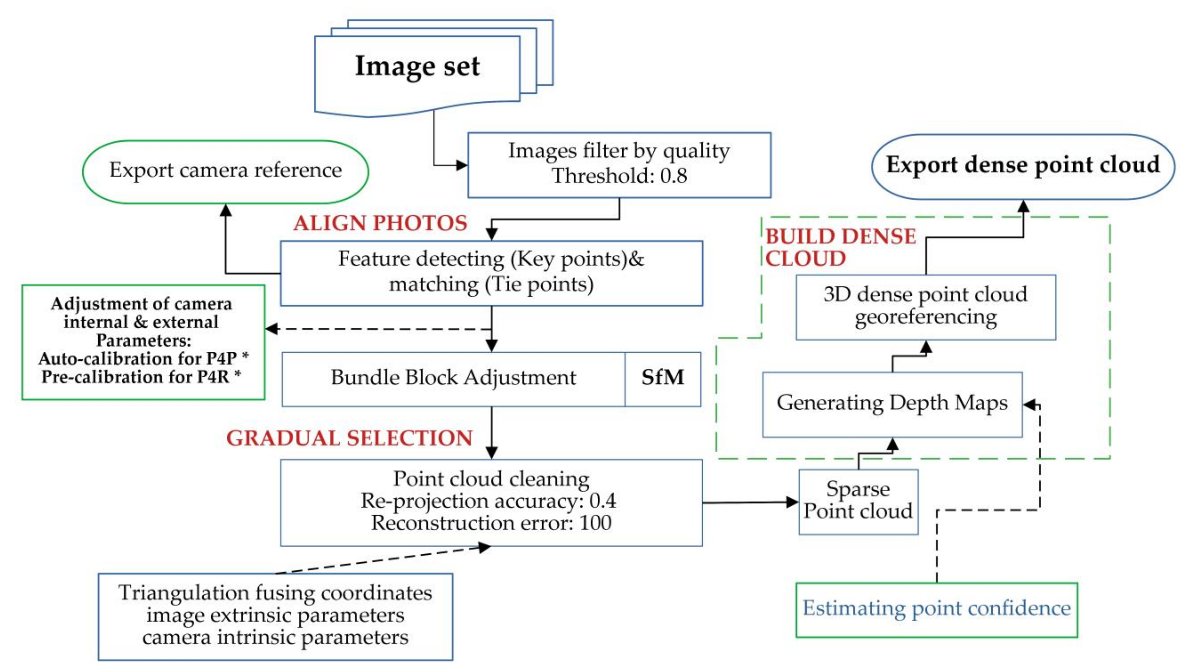
In this study, GNSS data were used to associate cloud points with coordinates during image binding. All geo-referenced data obtained by the GNSS receiver was recorded in the image taken by the camera. Metashape automatically reads the geo-referenced data. Before performing photo alignment, it was considered that motion-blurred images may be of low quality and affect the detection of image features throughout the mission. These images were removed in order not to affect the later generation of key points and tie points. Even though the flight parameters were determined based on preliminary tests in order to minimize the possibility of blur images, we still only retained the images with a quality score greater than 0.8 taking into account variations in climatic conditions on different flight dates. A generic preselection was performed for faster image matching in Metashape. Table S3 shows more detailed configuration parameters of P4P and P4R-based image processing in Metashape. Figure 3 shows the workflow for processing UAV-based images and generating and exporting point clouds.

After generating dense point clouds via Metashape, dense point clouds with unified local coordinates based on Metashape local space were exported as text files containing coordinate points and color information. All camera references calculated by Metashape were exported as a comma-separated text file for the purpose of accessing the proximity between the recorded coordinate information in images and results inferred from the photogrammetry.

2.4. Errors in the Georeferencing

Geospatial errors in the results of UAV photogrammetry, such as the Digital Surface Model (DSM) and the Digital Terrain Model (DEM), are typically assessed by the deployment of Ground Control Points (GCPs), whose coordinates are measured in advance by a high accuracy GNSS receiver [41,42]. GCPs with georeferenced information are used as control points or check points in UAV-based photogrammetry to improve and evaluate the errors [43]. In this study, GCPs were not applied, and in their place, five marks without accurate coordinate measurements were used as Manual Tie Points (MTPs), which can be used to assess and improve photogrammetry accuracy but not for geospatial error assessment. Each UAV image stores the original coordinate of the photographic location for the purpose of evaluating the georeferencing, which is a process in which the internal coordinate system of the UAV-image is related to the local coordinate system of photogrammetry. The coordinate data used for the photo alignment and can be reprojected. The reprojected location is based on the camera’s internal and external parameters, also denoted as theoretical locations. In order to discuss whether GNSS receivers mounted on UAVs with different accuracies affect the CHM, coordinates of the images captured by the DGPS-based P4P and RTK-based P4R platforms were used as aerial control points to relatively assess spatial errors. The original coordinates recorded by the different GNSS receivers deviated from the theoretical coordinates. The root mean square error (RMSE) [44] was used to assess the errors between the original and theoretical coordinates. In the case of this study, the RMSE of a one-dimensional variable was given by Equation (1).

$${\mathrm{RMSE}}_{\mathrm{a}}=\sqrt{\frac{{\sum }_{\mathrm{i}=1}^{\mathrm{N}}{\left({\mathrm{a}}^{\mathrm{i}}{}_{\mathrm{p}}-{\mathrm{a}}^{\mathrm{i}}{}_{\mathrm{o}}\right)}^2}{\mathrm{N}}}$$

(1)

where ${\mathrm{a}}^{\mathrm{i}}{}_{\mathrm{p}}$ and ${\mathrm{a}}^{\mathrm{i}}{}_{\mathrm{o}}$ are the i-th theoretical and originally measured values, respectively, and N is the total number of valid images. Generally, all data were divided into two dimensions to evaluate photogrammetry results, that is, planimetric and vertical data, respectively [45]. These RMSEs are computed as Equations (2) and (3), respectively.

$${\mathrm{RMSE}}_{\mathrm{h}}=\sqrt{\frac{{\sum }_{\mathrm{i}=1}^{\mathrm{N}}{\left({\mathrm{x}}^{\mathrm{i}}{}_{\mathrm{p}}-{\mathrm{x}}^{\mathrm{i}}{}_{\mathrm{o}}\right)}^2+{\left({\mathrm{y}}^{\mathrm{i}}{}_{\mathrm{p}}-{\mathrm{y}}^{\mathrm{i}}{}_{\mathrm{o}}\right)}^2}{\mathrm{N}}}$$

(2)

where ${\mathrm{RSME}}_{\mathrm{h}}$ represent the accuracy assessment of the horizontal direction; ${\mathrm{x}}^{\mathrm{i}}{}_{\mathrm{p}}$ and ${\mathrm{y}}^{\mathrm{i}}{}_{\mathrm{p}}$ are the i-th theoretical values of mutual vertical components corresponding to longitude and latitude, respectively, while ${\mathrm{x}}^{\mathrm{i}}{}_{\mathrm{o}}$ and ${\mathrm{y}}^{\mathrm{i}}{}_{\mathrm{o}}$ are originally measured values, and N is the total number of valid images.

$${\mathrm{RMSE}}_{\mathrm{v}}=\sqrt{\frac{{\sum }_{\mathrm{i}=1}^{\mathrm{N}}{\left({\mathrm{z}}^{\mathrm{i}}{}_{\mathrm{p}}-{\mathrm{z}}^{\mathrm{i}}{}_{\mathrm{o}}\right)}^2}{\mathrm{N}}}$$

(3)

where ${\mathrm{RSME}}_{\mathrm{v}}$ represents the accuracy assessment of the vertical direction; ${\mathrm{z}}^{\mathrm{i}}{}_{\mathrm{p}}$ and ${\mathrm{z}}^{\mathrm{i}}{}_{\mathrm{o}}$ are the i-th theoretical and originally measured values, respectively; N is the total number of valid images. Thus, the total RMSE of the space is calculated as shown in Equation (4).

$${\mathrm{RMSE}}_{\mathrm{t}}=\sqrt{\frac{{\mathrm{RMSE}}_{\mathrm{h}}{}^2+{\mathrm{RMSE}}_{\mathrm{v}}{}^2}{2}}$$

(4)

where ${\mathrm{RSME}}_{\mathrm{t}}$ represents the accuracy assessment of total space, ${\mathrm{RSME}}_{\mathrm{h}}$ represents the accuracy assessment of the horizontal direction; ${\mathrm{RSME}}_{\mathrm{v}}$ represents the accuracy assessment of the vertical direction.

2.5. Extraction of Point Clouds and Establishment of Crop Height Model (CHM) for Measured Height (MH) Estimation

In this study, crop MH was characterized as the average length between the upper boundary of rice panicle or blade and ground growth surface. MH was measured by a straight ruler in the paddy field. The Digital Surface Point Cloud (DSPC) is a model consisting of vegetation canopy and water surface cloud points, while the Digital Terrain Point Cloud (DTPC) represents the cloud points of ground surface without any vegetation. As shown in Figure 4b, since the camera mounted on the UAV may capture part of the non-canopy, the CHM data was often lower than those derived from MH, and this has been discussed in other relative studies [46]. The topographic point cloud with little straw residue points created by the images of paddy field without crop was used as the DTPC, that is, the growing point layer of the rice crop, which was acquired on 25 October 2020 (Figure 2e). The images acquired on other dates (the flight period: 16 July 2020–27 September 2020) (Figure 2a–d)) was used to create DSPCs, that is, the canopy points and water surface points. In previous studies, DSM has been used for crop canopy layer information and DTM for ground surface layer information [16,36,46].

The ground surface layer of the paddy field was not visible because flooding was required during rice growth (as shown in Figure 4c). In this case, to create the CHM, the invisible ground surface layer in DSPC can be approximately replaced by a DTPC created by the images taken on another date. In addition, estimating the height of submerged rice growth by measuring the depth of the water in the paddy field is another method used to create CHM. Therefore, two methods are proposed in this study based on the above. The images used for CHM creation are from the P4P and P4R, respectively. All point values of the original point cloud derived by Metashape are referenced with the WGS 84 geodetic coordinate system, which was converted into a local coordinate system and was further processed by open-source software, CloudCompare (v2.11 beta).

2.5.1. The Definition of M1 and M2

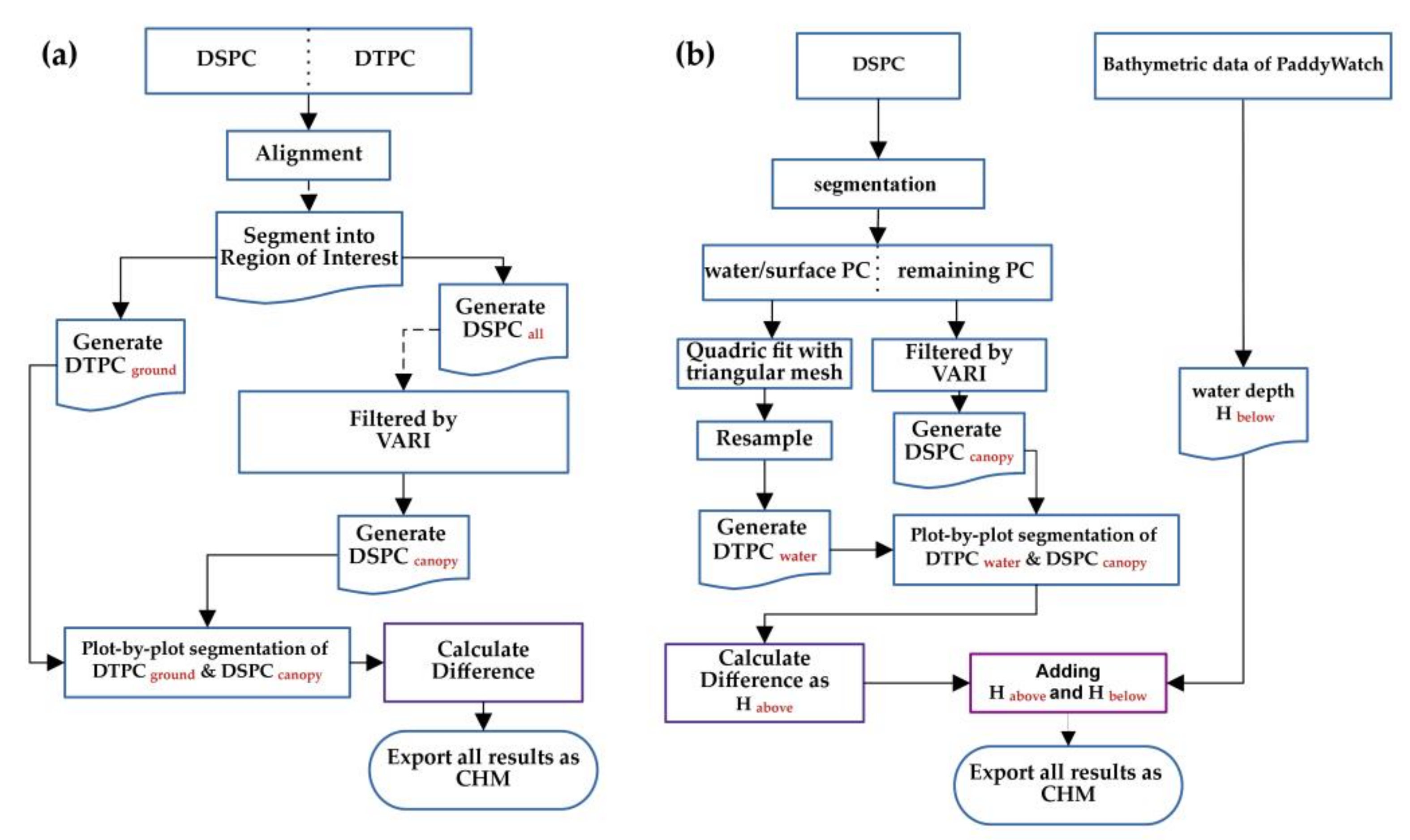
The alignment of DTPC and DSPC results in the digital cloud points of furrows and ridges in DTPC being in the same relative position as the digital cloud points for waterways and the rice canopy in DSPC, respectively. Figure 5 illustrates the definition for the construction of multi-temporal CHMs using the M1 method. The first method (M1) involves aligning the DTPC with the canopy layer of the DSPC filtered from the water surface and background noise and then calculating the difference between them to create the CHM, as shown in Figure 6a.

The second method (M2) involves segmenting the incomplete water surface cloud points in the DSPC and then fitting these points using a 2.5D quadric approach [47] to create an alternative complete water surface reference layer. The difference between this reference layer and the corresponding canopy layer (same as in M1) is calculated to obtain the rice CHM of the visible part above the water surface (Figure 4a). Subsequently, this was followed by the addition of water depth information recorded using a remote monitoring sensor, PaddyWatch (Vegetalia, inc.), as shown in Figure 1b, which is approximated to the height between the ground surface layer and the water surface layer (invisible part shown in Figure 4a) in order to get the complete CHM. The whole process is shown in Figure 6b.

2.5.2. Vegetation Index (VI) Filter and the Equations for the M1 and M2 Methods

The original DSPCs were generated by photogrammetry using RGB imagery taken in the period when the water fields were flooded. So, the DSPCs not only have canopy digital points but also water surface digital points (Figure 4c). All the points of the original DSPCs were applied into a VI filter to eliminate water background and other discrete noise points (Figure S1a–d). The VI filter is a threshold filter based on the Visible Atmospherically Resistant Index (VARI), which can be used in the visible portion of the spectrum to emphasize vegetation in the scene [48] while alleviating lighting differences and atmospheric effects. VARI is defined as shown in Equation (5) [49].

$$\mathrm{VARI}=\frac{{\mathrm{G}}_{\mathrm{DN}}-{\mathrm{R}}_{\mathrm{DN}}}{{\mathrm{G}}_{\mathrm{DN}}+{\mathrm{R}}_{\mathrm{DN}}-{\mathrm{B}}_{\mathrm{DN}}}$$

(5)

where ${\mathrm{G}}_{\mathrm{DN}}$, ${\mathrm{R}}_{\mathrm{DN}}$, and ${\mathrm{B}}_{\mathrm{DN}}$ represent the digital number (DN) of pixels in the red band, green band, and blue band for imagery. In general, to make images taken at different moments or on different dates comparable for the purpose of calculating VIs, the DN values recorded on the image pixels need to be radiometrically calibrated in order to calculate VI mapping based on reflectance [50,51]. In this study, since no such sunshine sensor or Downwelling Light sensors were installed on the P4P and P4R UAVs, as it was impossible to convert the images’ DN into reflectance. Given that each flight was carried out in sunny weather, and the flight times were within 10 min, we assume that there were roughly similar optical and atmospheric conditions between the images of each date, which indicated that the images captured from one flight in this study could be used to create VI. However, the images captured from different flights on different dates could not be compared. The DTPC and filtered DSPC (${\mathrm{DSPC}}_{\mathrm{canopy}}$) were aligned and then involved in the calculation of the CHM. The CHM of M1 was calculated as shown in Equation (6).

$${\mathrm{CHM}}_{\mathrm{M}1}={\mathrm{DSPC}}_{\mathrm{canopy}}-\mathrm{DTPC}$$

(6)

where ${\mathrm{CHM}}_{\mathrm{M}1}$ represents the crop height model of paddy rice created by the M1 method, and ${ \mathrm{DSPC}}_{\mathrm{canopy}}$ represents the filtered canopy digital cloud points of the rice crop surface layer; $\mathrm{DTPC}$ represents the digital cloud points of the topographic surface after harvesting.

In the M2 method, the water depth data, measured using a PaddyWatch sensor, and the DSPC were required simultaneously. Assuming no significant undulations in the ground surface layer of the paddy field, the CHM may be approximated as consisting of the height above the water and the water depth data. Therefore, the CHM of M2 is calculated as shown in Equations (7) and (8).

$${\mathrm{CHM}}_{\mathrm{M}2}={\mathrm{CH}}_{\mathrm{above}}+{\mathrm{WH}}_{\mathrm{depth} }$$

(7)

$${\mathrm{CH}}_{\mathrm{above}}{=\mathrm{DSPC}}_{\mathrm{canopy}}-{\mathrm{DSPC}}_{\mathrm{water} }$$

(8)

where ${\mathrm{CHM}}_{\mathrm{M}2}$ represents the crop height model of paddy rice created by M2 method; And ${\mathrm{CH}}_{\mathrm{above}}$ the CH above water; ${\mathrm{WH} }_{\mathrm{depth} }$ represents the water depth data of paddy field measured by PaddyWatch; ${\mathrm{DSPC}}_{\mathrm{canopy}}$ represents the filtered canopy digital cloud points of the rice crop surface layer; ${\mathrm{DSPC}}_{\mathrm{water} }$ represents the water surface digital point cloud.

2.6. Extraction and Analysis of Multispectral Information from P4M-Based Imagery

2.6.1. Vegetation Fraction (VF) and Canopy NDVI (${\mathrm{NDVI}}_{\mathrm{canopy}}$) Creation

All the images used to extract multispectral information were from the P4M, and the reflectance corresponding to the image DN were calculated using its onboard sunlight sensor. The reflectance is the ratio of the total radiation reflected from the object to the camera sensor to the total amount of radiation irradiated to the object. The NDVI was calculated as shown in Equation (9) [52].

$$\mathrm{NDVI}=\frac{{\mathrm{NIR}}_{\mathrm{reflectance}}-{\mathrm{Red}}_{\mathrm{reflectance}}}{{\mathrm{NIR}}_{\mathrm{reflectance}}+{\mathrm{Red}}_{\mathrm{reflectance}}}$$

(9)

where ${\mathrm{NIR}}_{\mathrm{reflectance}}$ represents the reflectivity value of the near-infrared band of the P4M, and ${\mathrm{Red}}_{\mathrm{reflectance}}$ represents the reflectivity value of the red band of the P4M. Pix4Dfields software (version 1.9.0), supported for the P4M UAV since Version 1.6.0 and which allows the improved processing of P4M-based images since Version 1.8.0, was used to process the original P4M-based multispectral images. The generated NDVI orthophoto is partially shown in Figure S2. Subsequently, the orthophoto was segmented and extracted plot by plot.

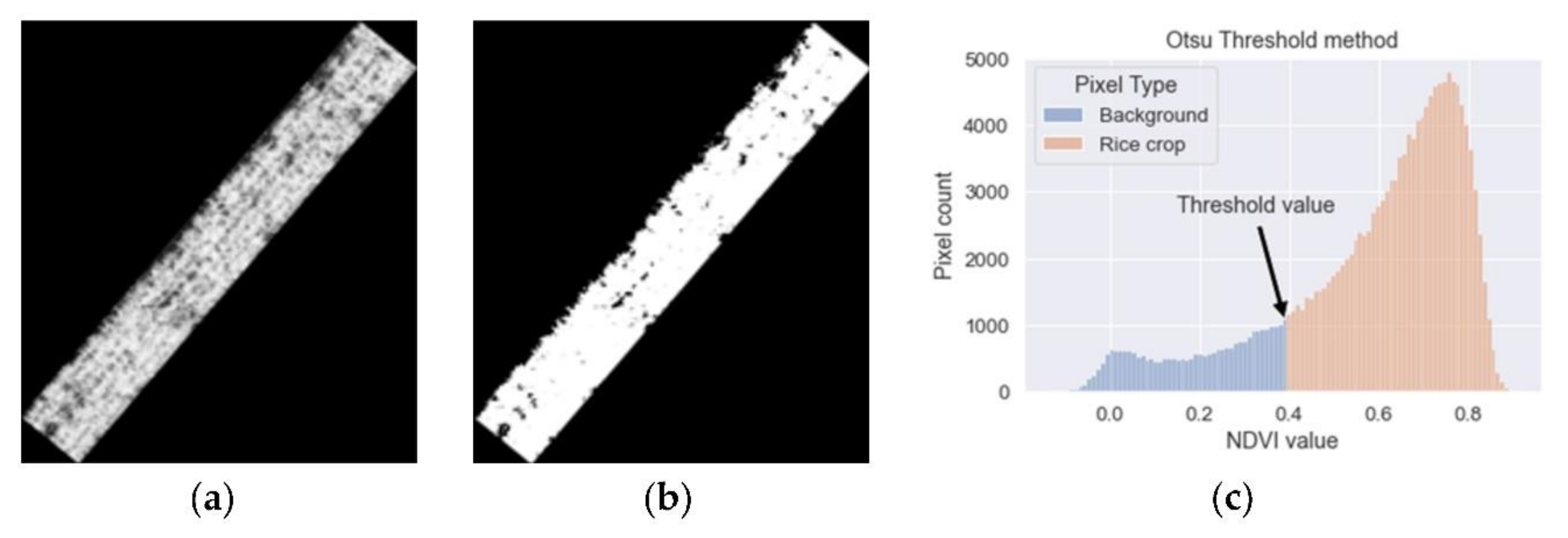
Where the VF and canopy the NDVI were calculated separately for each plot, the VF was defined as the percentage of vegetation within a certain area [53] on the NDVI orthophoto after thresholding by the NDVI value, and the canopy NDVI value (${\mathrm{NDVI}}_{\mathrm{canopy}}$) was defined as the average of the sum of NDVI values of pixels representing the rice canopy within the area. To quantify the VF and ${\mathrm{the} \mathrm{NDVI}}_{\mathrm{canopy}}$, regions of interest (ROI) (0.3 m × 28 m) [54,55] were selected in each plot (shown in Figure 7a,b) which also ensured most of the pixels of rice in each plot were selected.

In this study, each ROI was segmented by polygons so that it contained not only rice pixels but also background, such as water surface, pixels and did not fully represent the rice canopy layer. The Otsu thresholding algorithm was used to separate canopy pixels from the background of ROIs [56]. The Otsu method has been widely used for image information extraction and segmentation by minimizing the variance in order to calculate the best threshold relatively. The origial NDVI orthophoto is a gray-scale image, which can be binarized pixel by pixel by the Otsu method [54]. In the binary orthophoto, all pixels have only two possibilities, either 1 or 0. If the NDVI value equals or exceeds the threshold value defined by the Otus method, it is assigned a value of 1, i.e., it is considered to be vegetation. Conversely, if it is assigned a value of 0, it means that the NDVI value is less than the threshold value and is considered to be non-vegetation. The calculation of the VF in the ROI of each plot is shown in Equation (10). These data were obtained in bulk by running a Python (3.7.0, June 2018) script based on the open-source software development library OpenCV (4.5.1, December 2020) on QGIS (3.12.2-București), and the results are shown in Figure 7c. In addition, the accuracy of the Otsu method in this study was evaluated by comparison with manual identification [54].

$$\mathrm{VF}=\frac{{\mathrm{Pixel}}_{\mathrm{vegetation}}}{{\mathrm{Pixel}}_{\mathrm{total}}}$$

(10)

where VF represents the vegetation fraction, ${\mathrm{Pixel}}_{\mathrm{vegetation}}$ represents the vegetation part with value 1 by the Otsu method, that is, the total pixels of vegetation of the ROI, and ${\mathrm{Pixel}}_{\mathrm{total}}$ represents the total pixels of the ROI. The canopy NDVI value for each plot is also determined by the average pixel points within the Vegetation region of each ROI. The canopy NDVI is calculated as shown in Equation (11). In addition, to bring the NDVI of the rice canopy closer to the NDVI of rice leaf blades [57], a strict threshold was used for the partitioning of vegetation and non-vegetation in the ROI.

$${\mathrm{NDVI}}_{\mathrm{canopy}}=\frac{\sum {\mathrm{V}}_{\mathrm{vegetation}}}{{\mathrm{TP}}_{\mathrm{vegetation}}}$$

(11)

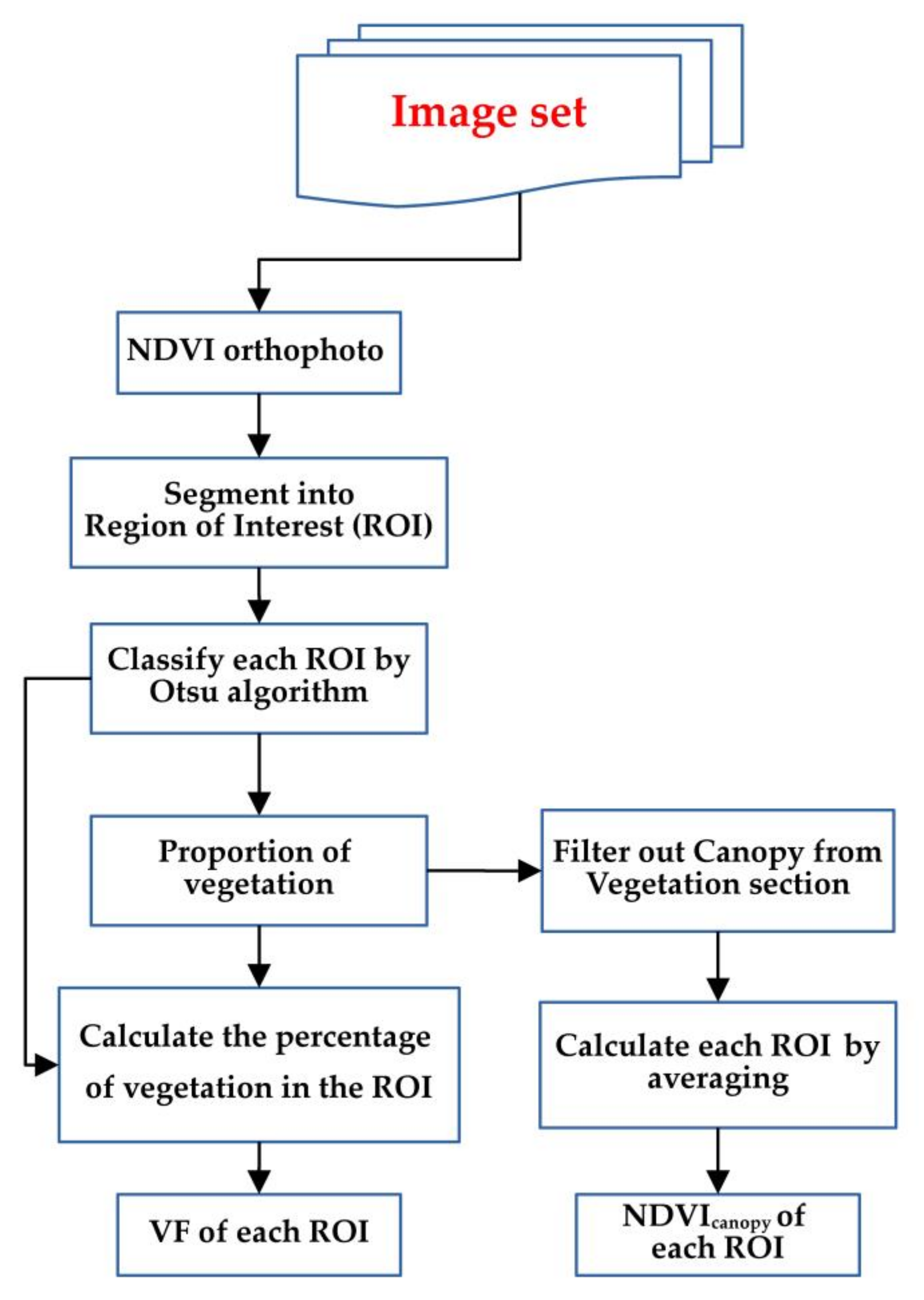
where ${\mathrm{NDVI}}_{\mathrm{canopy}}$ represents the average NDVI value of canopy; ${\mathrm{V}}_{\mathrm{vegetation}}$ represents the pixel value in the vegetation part; ${\mathrm{TP}}_{\mathrm{vegetation}}$ represents the total pixels of vegetation in the ROI. The extraction process for the VF and ${\mathrm{NDVI}}_{\mathrm{canopy}}$ is shown in Figure 8.

2.6.2. The Potential of the canopy NDVI (${\mathrm{NDVI}}_{\mathrm{canopy}}$), the Vegetation Fraction (VF), and the Soil Plant Analysis Development (SPAD) Value for Measured Height (MH) Estimation

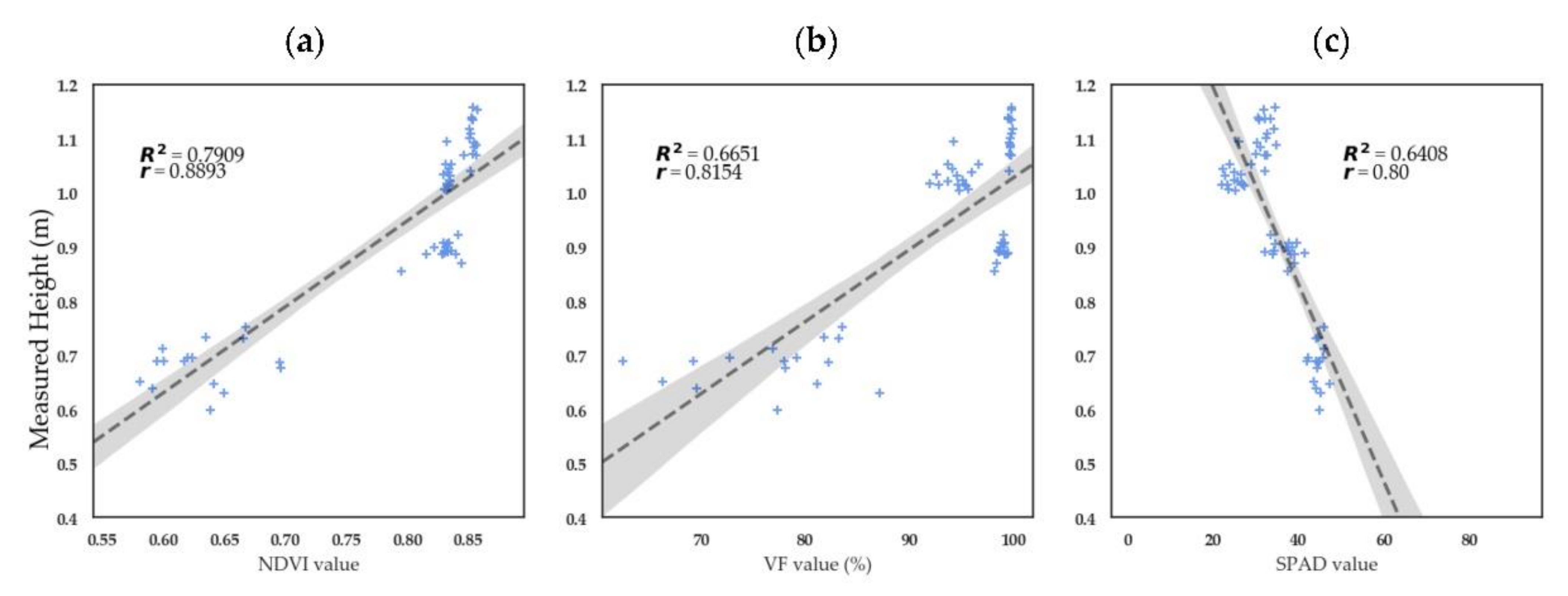
The Soil Plant Analysis Development (SPAD) of the rice leaf blade is another set of data obtained by manual measurements in the field. The SPAD is a commonly used CGS item in rice research that shows a high correlation with chlorophyll content. Therefore, the SPAD value has also been used to indicate the growth status of the crop [58]. Like the ${\mathrm{NDVI}}_{\mathrm{canopy}}$, the SPAD is calculated using the reflection and absorption of specific spectral bands by physiological structures in the crop. Previous research has shown that changes in the SPAD values of rice leaves during the growth period are negatively correlated with changes in height [59], and data from this study showed the same relationship, as shown in Figure 9c. In rice-related research, the NDVI was also often monitored as an essential growth indicator during rice growth [57,60]. The NDVI values increased as the rice tended to mature, while there was only a slight increase or decrease in NDVI values after reaching maturity [61]. The NDVI measurement approaches in previous studies are diverse, including remote sensing with satellites or UAV platforms [50,51,61]. Ref. [62] showed a modest correlation between NDVI and height in Italian ryegrass (${\mathrm{R}}^2=0.669$). The data from this study implied that the change in ${\mathrm{NDVI}}_{\mathrm{canopy}}$ values of canopy based on the ROIs of each plot was correlated with the change in MH, as shown in Figure 9a. The VF can also represent canopy cover, which generally increases with rice height, but it is unclear whether there is a linear relationship between CH and canopy cover changes. With the data extracted from Section 2.6.1, the linear relationship between the VF and MH is shown in Figure 9b.

As can be seen in the results shown in Figure 9, NDVI, VF, and leaf SPAD values show a certain correlation with MH. The ${\mathrm{NDVI}}_{\mathrm{canopy}}$ has the highest Pearson product–moment correlation coefficient with MH, with a positive correlation (0.8893). The correlation coefficient between the VF and the MH is positive at 0.80, while the SPAD value negatively correlates with MH at 0.8154. In the linear regression model, it can be seen that the estimated ${\mathrm{R}}^2$ of the ${\mathrm{NDVI}}_{\mathrm{canopy}}$ for MH reached 0.7909, while the estimates of the VF and the SPAD value for MH showed only a general regression correlation with an ${\mathrm{R}}^2$ of 0.6651 and 0.6408, respectively. Therefore, the M3 method was proposed for MH estimation using different combinations of the parameters, including ${\mathrm{NDVI}}_{\mathrm{canopy}} \mathrm{and} \mathrm{VF}$, ${\mathrm{SPAD} \mathrm{and} \mathrm{NDVI}}_{\mathrm{canopy}}$, $\mathrm{SPAD} \mathrm{and} \mathrm{VF}$, and ${\mathrm{SPAD} \mathrm{and} \mathrm{NDVI}}_{\mathrm{canopy}} \mathrm{and} \mathrm{VF}$.

2.7. Linear Regression and Corresponding Evaluation Metric

2.7.1. The Development of One-Dimensional Linear Regression

A one-dimensional linear regression model based on Ordinary Least Squares (OLS) [63] was used to analyze the relationship between the MH and the CHMs created by the M1 and M2 methods. The result was evaluated by the coefficient of determination. Generally, the CHM data was used to directly estimate the MH. The parsimonious Equation is shown as in Equation (12).

$${\mathrm{EH}}_x ~ \mathrm{A}\times \mathrm{MH}+\mathrm{B}$$

(12)

where ${\mathrm{EH}}_x$ represents the estimated rice height via CHM; $x$ represents the M1 or M2 method; $\mathrm{MH}$ represents the measured height in the field; A and B represent the estimates of the variable coefficient.

2.7.2. The Development of a Multiple Linear Regression (MLR) Model

The canopy NDVI, VF and SPAD values in Section 2.6.2 were used as variables to develop an MLR model, in which the variable coefficients were solved to implement models with different combinations of variables, as shown in Equation (13). Model diagnosis is a statistical prerequisite before building the MLR model. In this study, linearity between the independent and dependent variables, the normal distribution of the residuals, the homoscedasticity, and the correlation independence of the residuals were performed based on the data without significant outliers. All MLR analyses were performed in RStudio version 1.4.1103 (Copyright 2009–2021, PBC) with R package version 4.1.1. All data was divided into calibration and validation groups, and then k-fold cross-validation was used to validate the stability of the MLR model [38]. Four k-folds approaches were carried out, including: (1) 8-fold cross-validation, (2) 16-fold cross-validation, (3) 24-fold cross-validation, and (4) 32-fold cross-validation. Each fold was used as a single validation, while the remaining k-1 folds constituted the calibration group. The MH estimation models constructed by the k-1 folds calibration group were calculated one by one by repeated cross-validation with the 1-fold validation group and then averaged to obtain the cross-validation results.

$${\mathrm{EH}}_x ~ \mathrm{A}\times \mathrm{SPAD} +\mathrm{B}\times {\mathrm{NDVI}}_{\mathrm{canopy}}+\mathrm{C}\times \mathrm{VF}+\mathrm{D}$$

(13)

where ${\mathrm{EH}}_{\mathrm{x}}$ represents estimated height of rice via different combination variables, i.e., ${\mathrm{NDVI}}_{\mathrm{canopy}} \mathrm{and} \mathrm{VF}$, ${\mathrm{SPAD} \mathrm{and} \mathrm{NDVI}}_{\mathrm{canopy}}$, $\mathrm{SPAD} \mathrm{and} \mathrm{VF}$, and ${ \mathrm{SPAD} \mathrm{and} \mathrm{NDVI}}_{\mathrm{canopy}} \mathrm{and} \mathrm{VF}$; $\mathrm{SPAD}$, ${\mathrm{NDVI}}_{\mathrm{canopy}}$, and $\mathrm{VF}$ represent the parameters extracted from Section 2.6.2; and A, B, C, and D represent the estimates of each of the predictor variables, in which A or B or C can be zero to perform different MLR models.

The cross-validation results were further evaluated by the variation of ${\mathrm{R}}^2$, root mean squared error (RMSE) and mean absolute error (MAE). The variation is the difference of the corresponding metric between before and after cross-validation of the MLR model.

3. Results and Discussion

3.1. The Comparison of P4P-Based and P4R-Based Images of the Result of Error between Original and Theoretical Coordinates

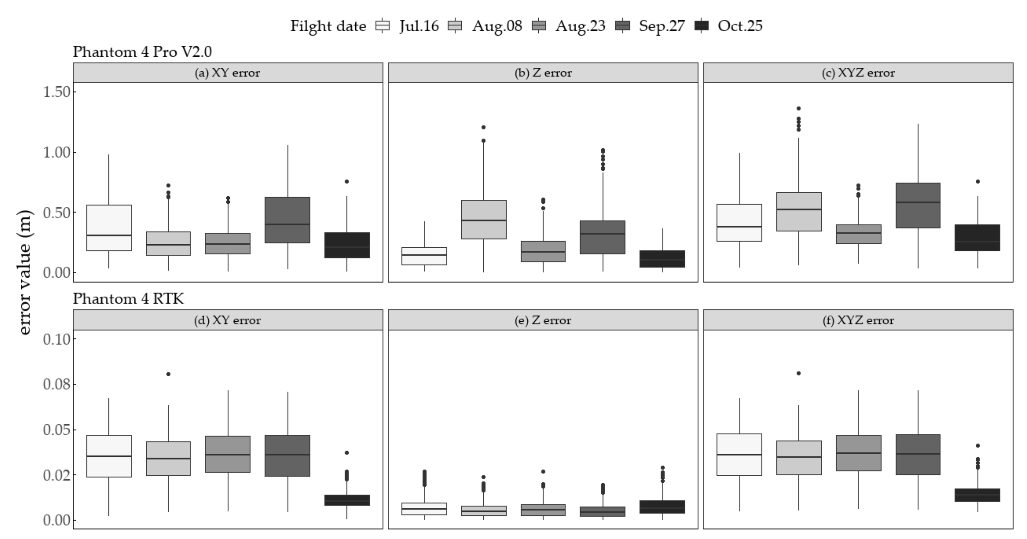
The image error was based on the theoretical location information of images estimated by the photogrammetry, coordinate, and altitude information recorded by the GNSS receiver during the UAV flight. The recorded coordinate information of UAV images was longitude and latitude based on the World Geodetic System 1984 (WGS84). The recorded altitude was based on WGS84 ellipsoid height. All errors were automatically calculated by Metashape software while implementing the photos alignment, before being exported. All image sets from five dates from 16 July 2020 to 25 October 2020 were separately analyzed, and the boxplot of corresponding error distribution is shown in Figure 10.

The RTK-based P4R image error range in total space is much lower than that of the DGPS-based P4P image error. The minimum planimetric error based on longitude and latitude was from 25 October 2020 in the cases of the P4P and P4R. The minimum vertical error based on altitude was also from 25 October 2020 in the case of the P4P. For total space error, the minimum values were obtained from 25 October 2020 in the cases of both the P4P and P4R. To further discuss the image error, RMSEs of errors in the planimetric and vertical and total spatial level of two UAVs were calculated manually, and the results are shown in

Table 2. The RMSE value between two UAVs (P4P and P4R) in images from different date sets in planimetric level (XY), vertical level (Z), and total spatial level (XYZ). All units of the results are cm.

Date	P4P			P4R
	XY RMSE	Z RMSE	XYZ RMSE	XY RMSE	Z RMSE	XYZ RMSE
16 July 2020	44	18	48	3.76	0.87	3.86
8 August 2020	28	51	58	3.67	0.68	3.73
23 August 2020	27	23	36	3.87	0.77	3.95
27 September 2020	50	38	63	3.86	0.66	3.92
25 October 2020	29	15	33	1.21	0.98	1.56

. The high error of the P4P-based images was expected and reasonable due to the limitation of the DPGS technique. The image error of this study was very close to the absolute positioning error of the DGPS (−50 cm) and the RTK-GNSS (−3 cm) receiver mounted on the P4P and P4R, respectively. In addition, similar to the results above, the image set obtained on 25 October 2020, when there was a bare paddy field after harvesting, had a lower amount of errors than other image sets obtained on other dates when there was rice growth.

3.2. The Results of the Performance of the Two Crop Height Models (CHMs)

The HMs obtained in the different plots were compared with the corresponding estimated CH of M1-based and M2-based CHMs extracted from P4P-based and P4R-based UAV photogrammetry, respectively. The four treatments in plots were low density without cover crop, low density with cover crop, high density without cover crop, and high density with cover crop, respectively (Figure S3).

3.2.1. The Relationship between Estimated Height of the M1 CHM and Measured Height (MH) in Different Treatments

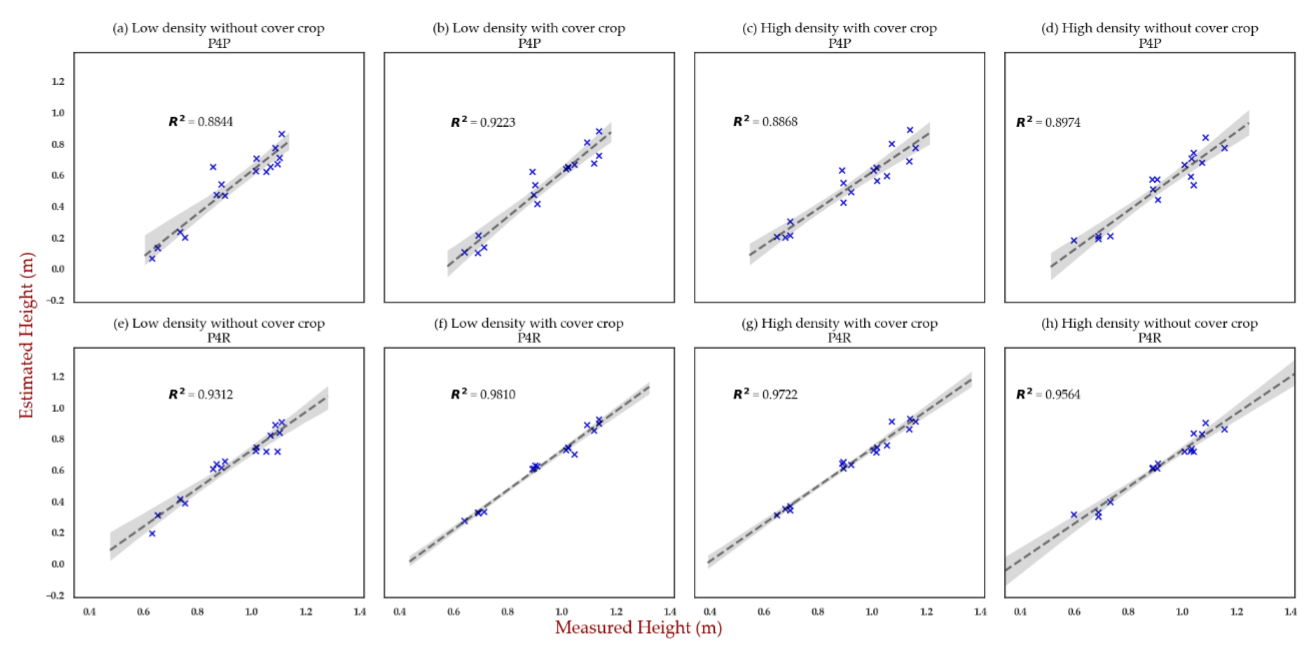
The linear relationship between the estimated height and MH based on the M1 method is shown in Figure 11.

In the M1 method, the estimated height and MH based on the P4P had high linear correlations where ${\mathrm{R}}^2$ reached 0.9223 in the treatment of low density with cover crop, and the lowest ${\mathrm{R}}^2$ value was obtained in the treatment of low density without cover crop, but it still was 0.8844. The ${\mathrm{R}}^2$ in the treatment of high density with cover crop and the treatment of high density without cover crop were 0.8868 and 0.8974, respectively. The results based on the P4R showed a better correlation compared to the P4R UAV, i.e., higher ${\mathrm{R}}^2$, where the treatment with the highest ${\mathrm{R}}^2$ was the low density with cover crop at 0.981 and the treatment with the lowest ${\mathrm{R}}^2$ value was the low density without cover crop at 0.9321, similarly to the case of the P4P. In the treatments of high density with cover crop, and high density without cover crop, meanwhile, the ${\mathrm{R}}^2$ was 0.9722 and 0.9564, respectively.

3.2.2. Relationship between the Estimated Height of the M2 CHM and Measured Height (MH) in Different Treatments

The linear relationship between the estimated height and MH created based on the M2 method is shown in Figure 12.

In the M2 method, the highest ${\mathrm{R}}^2$ of the linear model based on P4P-based photogrammetry was 0.9812 for the treatment of low density with cover crop, while the ${\mathrm{R}}^2$ of the remaining three treatments above were 0.9406 for low density with cover crop, 0.9736 for high density with cover crop, and 0.9548 for high density without cover crop. In the results of P4R-based photogrammetry, all four treatments were slightly less relevant than in the case of the P4P, with the highest ${\mathrm{R}}^2$ in the treatment of high density without cover crop at 0.9308. The other three treatments had an ${\mathrm{R}}^2$ of 0.866 for low density with cover crop, 0.9074 for high density with cover crop, and 0.9308 for low density without cover crop, respectively.

3.2.3. Overall Comparison of Performance between the M1-Based and M2-Based CHMs

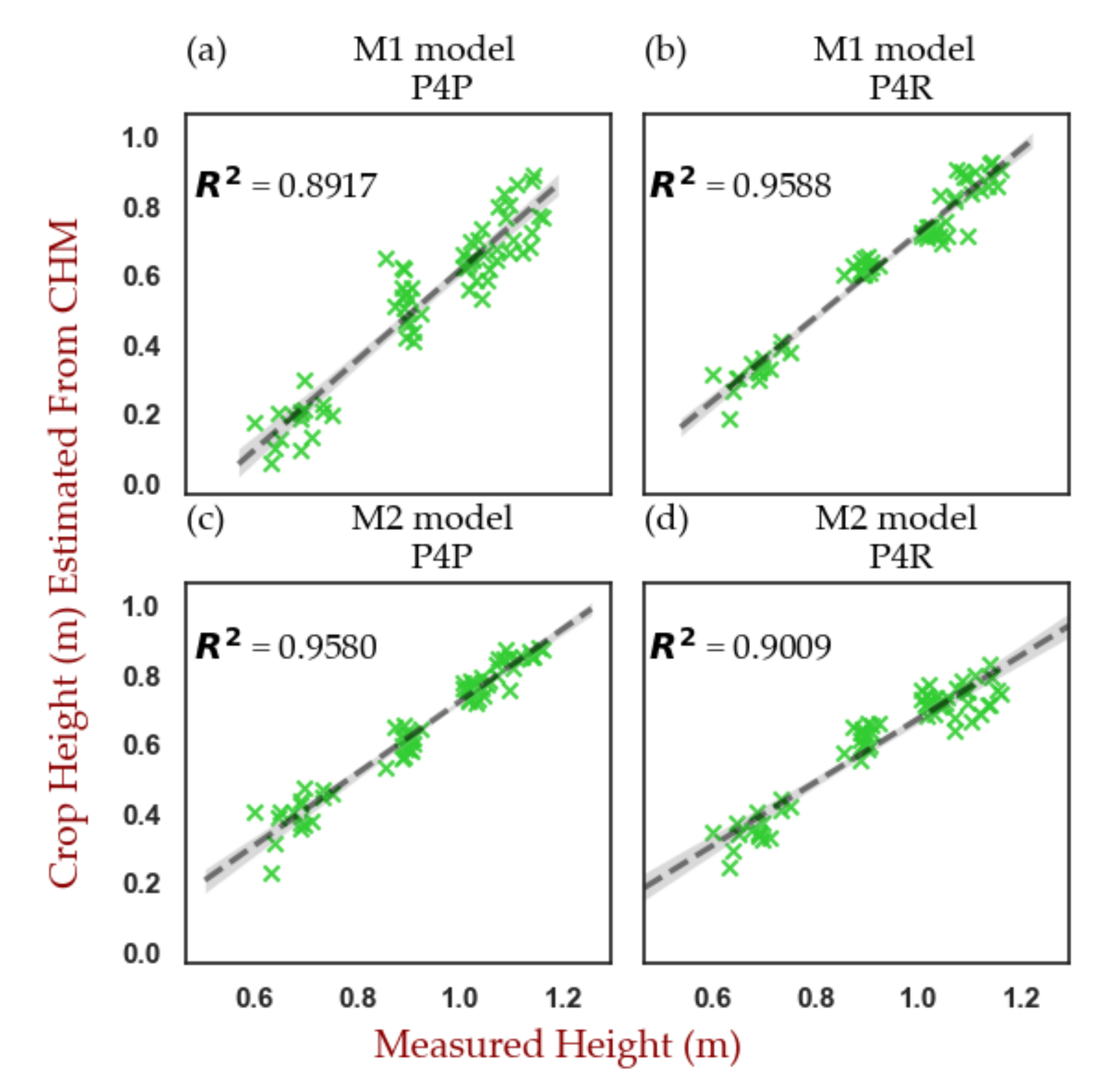
The results of Section 3.2.1 and Section 3.2.2 show that, based on the M1 and M2 methods, the linear correlation between estimated Crop Height (CH) and Measured Height (MH) on plots with different treatments is different. To further discuss the performance of M1 and M2 for estimating the overall CH of the paddy field under different UAV photogrammetry, all MH data were compared with the corresponding estimated CH obtained from CHM, and the results of the linear regression are shown in Figure 13.

For both the P4P and the P4R, the ${\mathrm{R}}^2$ between estimated CH and MH obtained based on the M1 and M2 method were relatively high. The ${\mathrm{R}}^2$ in the result based on the P4R is higher than that of the P4P using the M1 method, and vice versa with regard to M2 method. In the case of the P4R-based M1, the ${\mathrm{R}}^2$ is 0.958, while the P4P-based M1 is 0.8917. The ${\mathrm{R}}^2$ obtained by P4R and P4P-based M2 were 0.909 and 0.9580, respectively.

3.3. Canopy NDVI ($NDV{I}_{canopy}$), Vegetation Fraction (VF) and Soil Plant Analysis Development (SPAD) Associated with Chlorophyll Content for MH Estimation

The combination of the ${\mathrm{NDVI}}_{\mathrm{canopy}}$, VF and SPAD, were used as inputs for the MLR model to estimate MH, and the corresponding regression coefficients were analyzed for significance. All related results are shown in

Table 3. The details of MLR results of different combinations.

Assessed Variables	R2	T-Statistic Value			p-Value	Formula
		SPAD	NDVIcanopy	VF
SPAD and NDVIcanopy	0.838	***	***	-	***	1.139 × NDVIcanopy − 0.007 × SPAD + 0.288
SPAD and VF	0.817	***	-	***	***	0.81 × VF − 0.012 × SPAD + 0.584
NDVIcanopy and VF	0.807	-	***	*	***	2.254 × NDVIcanopy − 0.655 × VF − 0.24
SPAD and NDVIcanopy and VF	0.838	**	**	0.9	***	1.189 × NDVIcanopy − 0.007 × SPAD − 0.04 × VF + 0.281

Significance level at * 0.05, ** 0.01, and *** 0.001. -No parameter.

.

As can be seen from Table 3, the MLR models for all combinations are statistically significant after calibration. The MLR results of SPAD and ${\mathrm{NDVI}}_{\mathrm{canopy}}$ and SPAD and ${\mathrm{NDVI}}_{\mathrm{canopy}}$ and VF have equal highest ${\mathrm{R}}^2$ of 0.838, while the MLR result of SPAD and VF have an ${\mathrm{R}}^2$ of 0.817 and ${\mathrm{NDVI}}_{\mathrm{canopy}}$ and VF an ${\mathrm{R}}^2$ of 0.807. In terms of coefficient significance levels, the significance of the coefficients of ${\mathrm{NDVI}}_{\mathrm{canopy}}$ or VFs decreased in the case of VIs and VFs together, where, especially in the combination of SPAD and ${\mathrm{NDVI}}_{\mathrm{canopy}}$ and VF, the coefficient of VF did not have significance conditions, which means that the VF is redundant despite showing moderate correlation with MH data in the separate linear regression model. Taken together, the MLR model established by the combination of SPAD and ${\mathrm{NDVI}}_{\mathrm{canopy}}$ may be a potentially valid method (M3) to estimate MH based on the spectral data. To further study the performance of the M3 method for MH estimation in the paddy field, more validations of this model are needed.

3.4. The Performance of the M3 Method for Measured Height (MH) Estimation

3.4.1. The Cross-Validation Performance of the M3-Based MLR Model

Table 4. The evaluation metrics of MLR after 8-folds, 16-folds, 24-folds, and 32-folds cross-validation.

CV Method	${\mathbf{R}}^2$		RMSE (cm)	RMSE Variation (cm)	MAE (cm)	MAE Variation (cm)
	$\mathbf{Cross}-\mathbf{Validated} {\mathbf{R}}^2$	$\mathbf{Original} {\mathbf{R}}^2$
8-folds	0.827	0.838	5.9260	0.4658	−0.2233	−0.0295
16-folds	0.822	0.838	6.0018	0.4802	−0.2991	−0.0439
24-folds	0.829	0.838	5.8593	0.4601	−0.1566	−0.0238
32-folds	0.826	0.838	5.9475	0.4675	−0.2448	−0.0312

shows the cross-validation results of the MLR model analysis used for the MH, SPAD and NDVI. The main evaluation metrics include the change in ${\mathrm{R}}^2$, the change in root mean square error (RMSE), and the change in mean absolute error (MAE) before and after validation, and the results also show that the ${\mathrm{R}}^2$ changes at each k-fold are very small, with decreases within 0.9%–1.6%. On the other hand, the decrease in the RMSE of the model is about 5.8–6.0 cm. The variation based on MAE is very small, with a minimum of 0.1566 cm at 24 folds and a maximum of 0.2991 cm at 16 folds.

The cross-validation results show that different CV methods still robustly obtain an ${\mathrm{R}}^2$ of 0.822 to 0.829, which is not significantly different from the fitting data without cross-validation. Furthermore, ${\mathrm{R}}^2$, RMSE, and MAE are approximative under different k-folds. 8-fold, 16-fold, 24-fold, and 32-fold use 12.5%, 25%, 37.5%, and 50% of the overall block data, respectively. The results above show that the CV method has no significant impact on the validation of the MLR model using a combination of the SPAD value and canopy NDVI, which also indicates the reliability of the model at the statistical level.

3.4.2. Relationship between the Estimated Height of the M3 Model and Measured Height (MH) in Different Treatments

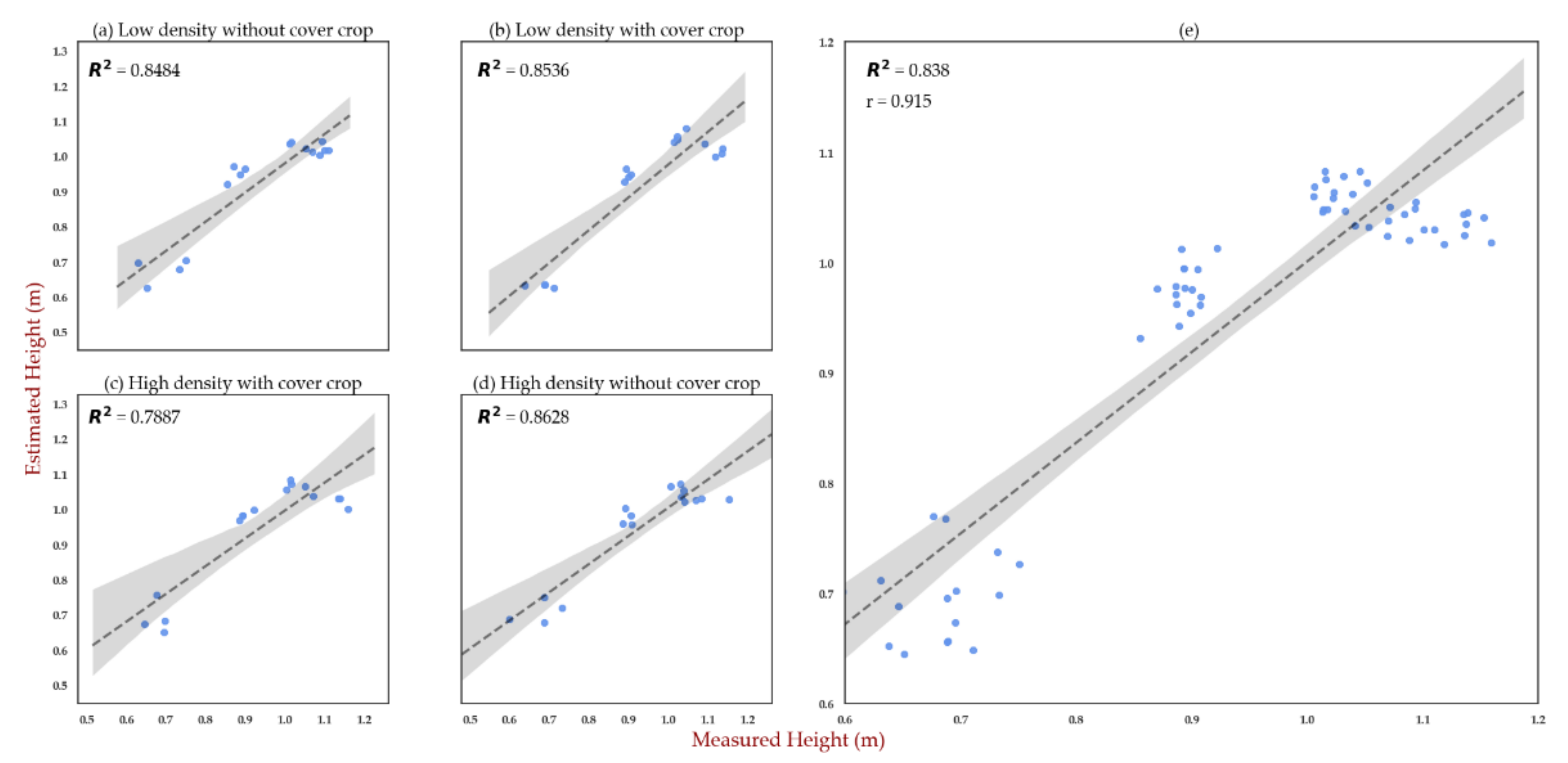
According to the result of Section 3.3, the MLR model based on the leaf SPAD value and canopy NDVI was used to evaluate MH in each separate plot and in the whole area. The results are shown in Figure 14. The ${\mathrm{R}}^2$ after MLR for the whole evaluation reached 0.838, a 16% improvement compared to the SPAD alone and a 3.5% improvement compared to the ${\mathrm{NDVI}}_{\mathrm{canopy}}$ (Figure 9), which indicates that the SPAD value (LCC content) and canopy NDVI together provide the potential for better MH estimation. When the MLR model was used to estimate the different plots with different treatments, high ${\mathrm{R}}^2$ of between 0.8484 to 0.8628 were obtained for most treatments, with high density with cover crop having a lower ${\mathrm{R}}^2$ of 0.7887 (Figure 14).

3.5. Evaluation and Discussion Based on the M1, M2, and M3 Methods

With regard to the performance of the models with different treatments, the M1 method obtained the highest correlation in the treatment of low density with cover crop and the lowest correlation in the treatment of low density without cover crop in the cases of both the P4P and P4R. The plot with low planting density and growth of green fertilizer crop in the waterway had a wider distribution of vegetation (Figure 13b) and had a lower homogeneity of vegetation per unit area compared to a high planting density (Figure 13d). In plots with cover crop, low density treatments showed better ${\mathrm{R}}^2$, which may be influenced by homogeneity [64], while in plots without cover crop, high density treatment showed higher ${ \mathrm{R}}^2$, which may be affected by the percentage of water regions; previous studies have also indicated that the water surface can have an impact on the accuracy of photogrammetry [65]. As in the case of the M1 method, in the M2 method, the treatment of low density without cover crop with a wider water region may have lead the higher uncertainty during UAV photogrammetry, and a higher density of vegetation in high density with cover crop may also have resulted in lower accuracy due to a high homogeneity of vegetation.

The P4P-based and P4R-based photogrammetry used the GNSS information recorded on the imagery during bundle adjustment, i.e., longitude, latitude, and altitude based on the WGS84, and then performed the georeferencing to map the WGS84-based location information for photogrammetry results, such as point clouds, DSM, DEM, and DTM. The GNSS information recorded tends to have some deviation from the absolute positioning information at that location due to errors in the GNSS receiver itself, which is also discussed in Section 3.1. In addition, the position information recorded by GNSS receivers was also biased when photography was performed at the same location on different dates. The relative misalignment of photogrammetry results in the Metashape workspace due to the bias of GNSS information between different image sets is referred to as relative spatial error (RSE) (e.g., Figure 15a). Previous studies have shown that the terrain detected by GNSS-based photogrammetry is subject to some distortions [66,67], i.e., deviations from the theoretical geodetic coordinate system-based terrain. The degree of deformation is absolute spatial stability (e.g., Figure 15b). The degree of identical trends in terrain deformation in photogrammetric results based on image sets taken on different dates is defined as relative spatial consistency (RSC) (e.g., Figure 15c). In photogrammetry for geomorphology, although terrain deformation occurred, the spatial information of the measured target in the scene may also be extracted with relative accuracy, defined as relative spatial stability. So, on the performance of the models in terms of the whole paddy field, the results of the M1 and M2 methods are different. In the M1 method, the CHMs of the P4R-based and P4P-based UAV photogrammetry were calculated from the DTPC and DSPCs, acquired at different dates, which needed to be aligned to minimize the effect of RSE due to errors from the GNSS receivers. The RSC of terrains reflected by the photogrammetry results from different sets of imagery at different dates may be the primary source of error in the aligned DTPC and DSPC for MH estimation. Tomaštík et al. [28] have shown that RTK/PPK techniques have the potential to achieve a similar degree of accuracy to GCPs, which are commonly used to improve the absolute spatial stability of terrain obtained by photogrammetry [66]. The high absolute spatial stability of the photogrammetry indicates a better RSC for the terrain of the same scene obtained at different dates. Therefore, the P4R-based photogrammetry is better for estimating MH than the P4P-based UAV photogrammetry in terms of the RSC of the terrain. In the M2 method, the RSE of the different results and the RSC are not the main influencing factors of the CHM since the CH estimated by the CHM is determined by the relative distance from the location of the canopy digital cloud points to the surrounding water surface digital cloud points derived by the DSPC and the values of the water level variation. As a sresult, the estimated CH based on M2 is mainly affected by the RSS of photogrammetry results. Notably, the P4P-based M2 obtained better MH estimation, indicating that the relative measurement of the scene target based on the P4P does not lose out to the P4R UAV without considering the geographic absolute spatial stability of terrain.

Unlike the comparison between height information in the M1 and M2 methods, the M3 method uses spectral information to estimate crop CH indirectly. Compared to the single factors discussed in Section 2.6.2., the model after multiple linear regression had better performance in estimating the overall crop CH in the paddy field. The SPAD value is calculated by red and infrared light transmission, which is dedicated to chlorophyll content [68]. The NDVI is then calculated from red and near- infrared light reflectance, which is designed for vegetation detection. So, it can be assumed that the trait of CH relates to leaf chlorophyII concentration and the overall NDVI of the canopy. Nevertheless, compared to the results obtained by the M1 and M2 methods, the ${\mathrm{R}}^2$ may be relatively low, which also implies that there may be more than two factors influencing the CH at the spectral level. However, when it comes to the performance with different treatments, except for the treatment of high density with cover crop, which showed a poor correlation, the remaining three treatments showed a higher ${\mathrm{R}}^2$ overall, close to the other two methods. It is assumed that more complex vegetation characteristics of the high density plot with cover crop resulted in higher uncertainties in the target areas throughout the UAV images. In addition, at the spectral level, the M3 method introduced red, infrared, and near-infrared lights into the estimation of CH, so developing a new spectral model dedicated to crop height estimation may be the next step to take.

4. Conclusions

The ground where flooded rice grows is difficult to detected directly by UAV-based photogrammetry. This study discussed the performance of consumer-grade UAV (P4P) equipment, professional-grade UAV equipped with a high-precision receiver (P4R), and a dedicated UAV (P4M) for multispectral analysis in order to estimate the CH of flooded rice during the growing season from different perspectives. All methods are feasible, which provides further possibilities when it comes to crop height estimation. Although the results with high ${\mathrm{R}}^2$ are obtained through these technologies, there are still some improvements needed. In terms of the M1 and M2 methods, the next step is to implement integrated and automated processes for capturing images in order to create a CHM model, instead of using stepped and cumbersome semi-automation. In the case of the M3 method, in order to further discuss whether there was an inherent relationship between such different phenotypes, i.e., height and multispectral information, more calibration and validation of that model are necessary. In addition, modeling crop height directly from more spectral information is a potential area of study.

References

1. Badawy, S.A.; Zayed, B.A.; Bassiouni, S.M.A.; Mahdi, A.H.A.; Majrashi, A.; Ali, E.F.; Seleiman, M.F. Influence of Nano Silicon and Nano Selenium on Root Characters, Growth, Ion Selectivity, Yield, and Yield Components of Rice (Oryza Sativa L.) under Salinity Conditions. Plants 2021, 10, 1657. [Google Scholar] [CrossRef] [PubMed]
2. Hossain, M.; Fischer, K.S. Rice Research for Food Security and Sustainable Agricultural Development in Asia: Achievements and Future Challenges. GeoJournal 1995, 35, 286–298. [Google Scholar] [CrossRef]
3. Gebbers, R.; Adamchuk, V.I. Precision Agriculture and Food Security. Science 2010, 327, 828–831. [Google Scholar] [CrossRef] [PubMed]
4. Yang, G.; Liu, J.; Zhao, C.; Li, Z.; Huang, Y.; Yu, H.; Xu, B.; Yang, X.; Zhu, D.; Zhang, X.; et al. Unmanned Aerial Vehicle Remote Sensing for Field-Based Crop Phenotyping: Current Status and Perspectives. Front. Plant Sci. 2017, 8, 1111. [Google Scholar] [CrossRef]
5. Fasoula, V.A.; Fasoula, D.A. Principles Underlying Genetic Improvement for High and Stable Crop Yield Potential. Field Crops Res. 2002, 75, 191–209. [Google Scholar] [CrossRef]
6. Darvishzadeh, R.; Skidmore, A.; Schlerf, M.; Atzberger, C. Inversion of a Radiative Transfer Model for Estimating Vegetation LAI and Chlorophyll in a Heterogeneous Grassland. Remote Sens. Environ. 2008, 112, 2592–2604. [Google Scholar] [CrossRef]
7. Yu, K.; Lenz-Wiedemann, V.; Chen, X.; Bareth, G. Estimating Leaf Chlorophyll of Barley at Different Growth Stages Using Spectral Indices to Reduce Soil Background and Canopy Structure Effects. ISPRS J. Photogramm. Remote Sens. 2014, 97, 58–77. [Google Scholar] [CrossRef]
8. Li, B.; Xu, X.; Han, J.; Zhang, L.; Bian, C.; Jin, L.; Liu, J. The Estimation of Crop Emergence in Potatoes by UAV RGB Imagery. Plant Methods 2019, 15, 15. [Google Scholar] [CrossRef] [Green Version]
9. Madec, S.; Baret, F.; de Solan, B.; Thomas, S.; Dutartre, D.; Jezequel, S.; Hemmerlé, M.; Colombeau, G.; Comar, A. High-Throughput Phenotyping of Plant Height: Comparing Unmanned Aerial Vehicles and Ground LiDAR Estimates. Front. Plant Sci. 2017, 8, 2002. [Google Scholar] [CrossRef] [Green Version]
10. Li, W.; Niu, Z.; Chen, H.; Li, D.; Wu, M.; Zhao, W. Remote Estimation of Canopy Height and Aboveground Biomass of Maize Using High-Resolution Stereo Images from a Low-Cost Unmanned Aerial Vehicle System. Ecol. Indic. 2016, 67, 637–648. [Google Scholar] [CrossRef]
11. Casanova, D.; Epema, G.F.; Goudriaan, J. Monitoring Rice Reflectance at Field Level for Estimating Biomass and LAI. Field Crops Res. 1998, 55, 83–92. [Google Scholar] [CrossRef]
12. Liu, X.; Zhai, H.; Shen, Y.; Lou, B.; Jiang, C.; Li, T.; Hussain, S.B.; Shen, G. Large-Scale Crop Mapping From Multisource Remote Sensing Images in Google Earth Engine. IEEE J. Sel. Top. Appl. Earth Obs. Remote Sens. 2020, 13, 414–427. [Google Scholar] [CrossRef]
13. Chang, A.; Eo, Y.; Kim, S.; Kim, Y.; Kim, Y. Canopy-Cover Thematic-Map Generation for Military Map Products Using Remote Sensing Data in Inaccessible Areas. Landsc. Ecol. Eng. 2010, 7, 263–274. [Google Scholar] [CrossRef]
14. Mulla, D.J. Twenty Five Years of Remote Sensing in Precision Agriculture: Key Advances and Remaining Knowledge Gaps. Biosyst. Eng. 2013, 114, 358–371. [Google Scholar] [CrossRef]
15. Radoglou-Grammatikis, P.; Sarigiannidis, P.; Lagkas, T.; Moscholios, I. A Compilation of UAV Applications for Precision Agriculture. Comput. Netw. 2020, 172, 107148. [Google Scholar] [CrossRef]
16. Chang, A.; Jung, J.; Maeda, M.M.; Landivar, J. Crop Height Monitoring with Digital Imagery from Unmanned Aerial System (UAS). Comput. Electron. Agric. 2017, 141, 232–237. [Google Scholar] [CrossRef]
17. Bonadies, S.; Lefcourt, A.; Gadsden, S.A. A Survey of Unmanned Ground Vehicles with Applications to Agricultural and Environmental Sensing. In Proceedings of the Autonomous Air and Ground Sensing Systems for Agricultural Optimization and Phenotyping, Baltimore, MD, USA, 18–19 April 2016; Volume 9866, pp. 142–155. [Google Scholar]
18. Han-Ya, I.; Ishii, K.; Noguchi, N. Satellite and Aerial Remote Sensing for Production Estimates and Crop Assessment. Environ. Control. Biol. 2010, 48, 51–58. [Google Scholar] [CrossRef] [Green Version]
19. Gevaert, C.M.; Suomalainen, J.; Tang, J.; Kooistra, L. Generation of Spectral–Temporal Response Surfaces by Combining Multispectral Satellite and Hyperspectral UAV Imagery for Precision Agriculture Applications. IEEE J. Sel. Top. Appl. Earth Obs. Remote Sens. 2015, 8, 3140–3146. [Google Scholar] [CrossRef]
20. Araus, J.L.; Cairns, J.E. Field High-Throughput Phenotyping: The New Crop Breeding Frontier. Trends Plant Sci. 2014, 19, 52–61. [Google Scholar] [CrossRef]
21. Gil-Docampo, M.L.; Arza-García, M.; Ortiz-Sanz, J.; Martínez-Rodríguez, S.; Marcos-Robles, J.L.; Sánchez-Sastre, L.F. Above-Ground Biomass Estimation of Arable Crops Using UAV-Based SfM Photogrammetry. Geocarto Int. 2020, 35, 687–699. [Google Scholar] [CrossRef]
22. Bendig, J.; Bolten, A.; Bennertz, S.; Broscheit, J.; Eichfuss, S.; Bareth, G. Estimating Biomass of Barley Using Crop Surface Models (CSMs) Derived from UAV-Based RGB Imaging. Remote Sens. 2014, 6, 10395. [Google Scholar] [CrossRef] [Green Version]
23. Torres-Sánchez, J.; Peña, J.M.; de Castro, A.I.; López-Granados, F. Multi-Temporal Mapping of the Vegetation Fraction in Early-Season Wheat Fields Using Images from UAV. Comput. Electron. Agric. 2014, 103, 104–113. [Google Scholar] [CrossRef]
24. Xuan, W.; Lin, Z. Rectifying High-Resolution Images by Using Rectified Low-Resolution Images. In Multispectral Image Processing and Pattern Recognition; International Society for Optics and Photonics: Wuhan, China, 2001; Volume 4552, pp. 196–200. [Google Scholar]
25. Stempfhuber, W.; Buchholz, M. A Precise, Low-Cost Rtk Gnss System for Uav Applications. Int. Arch. Photogramm. Remote Sens. Spatial Inf. Sci. 2012, XXXVIII-1/C22, 289–293. [Google Scholar] [CrossRef] [Green Version]
26. Gerke, M.; Przybilla, H.J. Accuracy Analysis of Photogrammetric UAV Image Blocks: Influence of Onboard RTK-GNSS and Cross Flight Patterns. Photogramm Fernerkun 2016, 17–30. [Google Scholar] [CrossRef] [Green Version]
27. Štroner, M.; Urban, R.; Seidl, J.; Reindl, T.; Brouček, J. Photogrammetry Using UAV-Mounted GNSS RTK: Georeferencing Strategies without GCPs. Remote Sens. 2021, 13, 1336. [Google Scholar] [CrossRef]
28. Tomaštík, J.; Mokroš, M.; Surový, P.; Grznárová, A.; Merganič, J. UAV RTK/PPK Method—An Optimal Solution for Mapping Inaccessible Forested Areas? Remote Sens. 2019, 11, 721. [Google Scholar] [CrossRef] [Green Version]
29. Jaud, M.; Bertin, S.; Beauverger, M.; Augereau, E.; Delacourt, C. RTK GNSS-Assisted Terrestrial SfM Photogrammetry without GCP: Application to Coastal Morphodynamics Monitoring. Remote Sens. 2020, 12, 1889. [Google Scholar] [CrossRef]
30. Bannari, A.; Morin, D.; Bonn, F.; Huete, A.R. A Review of Vegetation Indices. Remote Sens. Rev. 1995, 13, 95–120. [Google Scholar] [CrossRef]
31. Jakubauskas, M.E.; Legates, D.R.; Kastens, J.H. Crop Identification Using Harmonic Analysis of Time-Series AVHRR NDVI Data. Comput. Electron. Agric. 2002, 37, 127–139. [Google Scholar] [CrossRef]
32. Davi, H.; Soudani, K.; Deckx, T.; Dufrene, E.; Le Dantec, V.; FranÇois, C. Estimation of Forest Leaf Area Index from SPOT Imagery Using NDVI Distribution over Forest Stands. Int. J. Remote Sens. 2006, 27, 885–902. [Google Scholar] [CrossRef]
33. Freden, S.C.; Mercanti, E.P.; Becker, M.A. Third Earth Resources Technology Satellite-1 Symposium: The Proceedings of a Symposium Held by Goddard Space Flight Center at Washington, D.C. on December 10–14, 1973: Prepared at Goddard Space Flight Center; National Aeronautics and Space Administration: Greenbelt, MD, USA, 1974; Volume 3, pp. 1–155. [Google Scholar]
34. Villareal, M.K.; Tongco, A.F.; Maja, J.M.J. Winter Wheat Crop Height Estimation Using Small Unmanned Aerial System (SUAS). Agric. Sci. 2020, 11, 355–368. [Google Scholar] [CrossRef] [Green Version]
35. GISGeography. DEM, DSM & DTM Differences-A Look at Elevation Models in GIS. Available online: https://gisgeography.com/dem-dsm-dtm-differences/ (accessed on 18 November 2021).
36. Malambo, L.; Popescu, S.C.; Murray, S.C.; Putman, E.; Pugh, N.A.; Horne, D.W.; Richardson, G.; Sheridan, R.; Rooney, W.L.; Avant, R.; et al. Multitemporal Field-Based Plant Height Estimation Using 3D Point Clouds Generated from Small Unmanned Aerial Systems High-Resolution Imagery. Int. J. Appl. Earth Obs. Geoinf. 2018, 64, 31–42. [Google Scholar] [CrossRef]
37. Wang, X.; Zhang, R.; Song, W.; Han, L.; Liu, X.; Sun, X.; Luo, M.; Chen, K.; Zhang, Y.; Yang, H.; et al. Dynamic Plant Height QTL Revealed in Maize through Remote Sensing Phenotyping Using a High-Throughput Unmanned Aerial Vehicle (UAV). Sci. Rep. 2019, 9, 3458. [Google Scholar] [CrossRef] [PubMed] [Green Version]
38. Gebremedhin, A.; Badenhorst, P.; Wang, J.; Giri, K.; Spangenberg, G.; Smith, K. Development and Validation of a Model to Combine NDVI and Plant Height for High-Throughput Phenotyping of Herbage Yield in a Perennial Ryegrass Breeding Program. Remote Sens. 2019, 11, 2494. [Google Scholar] [CrossRef] [Green Version]
39. Kawamura, K.; Asai, H.; Yasuda, T.; Khanthavong, P.; Soisouvanh, P.; Phongchanmixay, S. Field Phenotyping of Plant Height in an Upland Rice Field in Laos Using Low-Cost Small Unmanned Aerial Vehicles (UAVs). Plant Prod. Sci. 2020, 23, 452–465. [Google Scholar] [CrossRef]
40. Jimenez-Berni, J.A.; Deery, D.M.; Rozas-Larraondo, P.; Condon, A.; Tony, G.; Rebetzke, G.J.; James, R.A.; Bovill, W.D.; Furbank, R.T.; Sirault, X.R.R. High Throughput Determination of Plant Height, Ground Cover, and Above-Ground Biomass in Wheat with LiDAR. Front. Plant Sci. 2018, 9, 237. [Google Scholar] [CrossRef] [PubMed] [Green Version]
41. Uysal, M.; Toprak, A.S.; Polat, N. DEM Generation with UAV Photogrammetry and Accuracy Analysis in Sahitler Hill. Measurement 2015, 73, 539–543. [Google Scholar] [CrossRef]
42. Gonçalves, J.A.; Henriques, R. UAV Photogrammetry for Topographic Monitoring of Coastal Areas. ISPRS J. Photogramm. Remote Sens. 2015, 104, 101–111. [Google Scholar] [CrossRef]
43. Agisoft. Control and Check Points for Aerial Surveys. Available online: https://agisoft.freshdesk.com/support/solutions/articles/31000154132-control-and-check-points-for-aerial-surveys (accessed on 18 November 2021).
44. Wikipedia. Root-Mean-Square Deviation. Available online: https://en.wikipedia.org/wiki/Root-mean-square_deviation (accessed on 19 November 2021).
45. Peppa, M.V.; Hall, J.; Goodyear, J.; Mills, J.P. Photogrammetric Assessment and Comparison of Dji Phantom 4 Pro and Phantom 4 Rtk Small Unmanned Aircraft Systems. Int. Arch. Photogramm. Remote Sens. Spatial Inf. Sci. 2019, XLII-2/W13, 503–509. [Google Scholar] [CrossRef] [Green Version]
46. Han, X.; Thomasson, J.A.; Bagnall, G.C.; Pugh, N.A.; Horne, D.W.; Rooney, W.L.; Jung, J.; Chang, A.; Malambo, L.; Popescu, S.C.; et al. Measurement and Calibration of Plant-Height from Fixed-Wing UAV Images. Sensors 2018, 18, 4092. [Google Scholar] [CrossRef] [Green Version]
47. CloudCompareWiki. Fit Quadric-CloudCompareWiki. Available online: https://www.cloudcompare.org/doc/wiki/index.php?title=Fit_Quadric (accessed on 26 November 2021).
48. Afdhalia, F.; Supriatna, S.; Shidiq, I.P.A.; Manessa, M.D.M.; Ristya, Y. Detection of Rice Varieties Based on Spectral Value Data Using UAV-Based Images. In Proceedings of the Sixth International Symposium on LAPAN-IPB Satellite, Bogor, Indonesia, 17–18 September 2019; Volume 1137222. [Google Scholar] [CrossRef]
49. Gitelson, A.A.; Stark, R.; Grits, U.; Rundquist, D.; Kaufman, Y.; Derry, D. Vegetation and Soil Lines in Visible Spectral Space: A Concept and Technique for Remote Estimation of Vegetation Fraction. Int. J. Remote Sens. 2002, 23, 2537–2562. [Google Scholar] [CrossRef]
50. Cao, Y.; Li, G.L.; Luo, Y.K.; Pan, Q.; Zhang, S.Y. Monitoring of Sugar Beet Growth Indicators Using Wide-Dynamic-Range Vegetation Index (WDRVI) Derived from UAV Multispectral Images. Comput. Electron. Agric. 2020, 171, 105331. [Google Scholar] [CrossRef]
51. Rosle, R.; Che’Ya, N.; Roslin, N.; Halip, R.; Ismail, M. Monitoring Early Stage of Rice Crops Growth Using Normalized Difference Vegetation Index Generated from UAV. IOP Conf. Ser. Earth Environ. Sci. 2019, 355, 012066. [Google Scholar] [CrossRef]
52. Huang, S.; Tang, L.; Hupy, J.P.; Wang, Y.; Shao, G. A Commentary Review on the Use of Normalized Difference Vegetation Index (NDVI) in the Era of Popular Remote Sensing. J. For. Res. 2021, 32, 1–6. [Google Scholar] [CrossRef]
53. Purevdorj, T.S.; Tateishi, R.; Ishiyama, T.; Honda, Y. Relationships between Percent Vegetation Cover and Vegetation Indices. Int. J. Remote Sens. 1998, 19, 3519–3535. [Google Scholar] [CrossRef]
54. Kim, D.-W.; Yun, H.; Jeong, S.-J.; Kwon, Y.-S.; Kim, S.-G.; Lee, W.; Kim, H.-J. Modeling and Testing of Growth Status for Chinese Cabbage and White Radish with UAV-Based RGB Imagery. Remote Sens. 2018, 10, 563. [Google Scholar] [CrossRef] [Green Version]
55. Yang, H.; Yang, X.; Heskel, M.; Sun, S.; Tang, J. Seasonal Variations of Leaf and Canopy Properties Tracked by Ground-Based NDVI Imagery in a Temperate Forest. Sci. Rep. 2017, 7, 1267. [Google Scholar] [CrossRef]
56. Otsu, N. A Threshold Selection Method from Gray-Level Histograms. IEEE Trans. Syst. Man Cybern. 1979, 9, 62–66. [Google Scholar] [CrossRef] [Green Version]
57. Fenghua, Y.; Tongyu, X.; Yingli, C.; Guijun, Y.; Wen, D.; Shu, W. Models for Estimating the Leaf NDVI of Japonica Rice on a Canopy Scale by Combining Canopy NDVI and Multisource Environmental Data in Northeast China. Int. J. Agric. Biol. Eng. 2016, 9, 132–142. [Google Scholar]
58. Kimani, S.M.; Cheng, W.; Kanno, T.; Nguyen-Sy, T.; Abe, R.; Oo, A.Z.; Tawaraya, K.; Sudo, S. Azolla Cover Significantly Decreased CH 4 but Not N 2 O Emissions from Flooding Rice Paddy to Atmosphere. Soil Sci. Plant Nutr. 2018, 64, 68–76. [Google Scholar] [CrossRef] [Green Version]
59. Hussain, S.; Fujii, T.; McGoey, S.; Yamada, M.; Ramzan, M.; Akmal, M. Evaluation of Different Rice Varieties for Growth and Yield Characteristics. J. Anim. Plant Sci. 2014, 24, 1504–1510. [Google Scholar]
60. Liu, K.; Li, Y.; Hu, H. Predicting Ratoon Rice Growth Rhythmbased on NDVI at Key Growth Stages of Main Rice. Chil. J. Agric. Res. 2015, 75, 410–417. [Google Scholar] [CrossRef] [Green Version]
61. Minh, V.Q.; Hien, T.T.; Chien, H.V. Monitoring and Delineating the Progress of Rice Sowing and Cropping Calendar Assisting in Early Warning Pest and Desease in the Mekong Delta. In Proceedings of the 34th Asian Conference on Remote Sensing (ACRS 2013), Bali, Indonesia, 20–24 October 2013; p. 8. [Google Scholar]
62. Rahetlah, B.V.; Salgado, P.; Andrianarisoa, B.; Tillard, E.; Razafindrazaka, H.; Mézo, L.L.; Ramalanjaona, V.L. Relationship between Normalized Difference Vegetation Index (NDVI) and Forage Biomass Yield in the Vakinankaratra Region, Madagascar. Livest. Res. Rural. Dev. 2014, 26, 95. [Google Scholar]
63. Wikipedia. Ordinary Least Squares. Scientific and Technical Information Office, National Aeronautics and Space Administration.
64. Pepe, M.; Ackermann, S.; Fregonese, L.; Achille, C. 3D Point Cloud Model Color Adjustment by Combining Terrestrial Laser Scanner and Close Range Photogrammetry Datasets. In Proceedings of the ICDH 2016: 18th International Conference on Digital Heritage, London, UK, 24–25 November 2016; Volume 10, p. 7. [Google Scholar]
65. Westaway, R.M. Remote Sensing of Clear-Water, Shallow, Gravel-Bed Rivers Using Digital Photogrammetry. Photogramm. Eng. 2001, 67, 1271–1282. [Google Scholar]
66. Ruzgienė, B.; Berteška, T.; Gečyte, S.; Jakubauskienė, E.; Aksamitauskas, V.Č. The Surface Modelling Based on UAV Photogrammetry and Qualitative Estimation. Measurement 2015, 73, 619–627. [Google Scholar] [CrossRef]
67. Marek, L.; Miřijovský, J.; Tuček, P. Monitoring of the Shallow Landslide Using UAV Photogrammetry and Geodetic Measurements. In Proceedings of the Engineering Geology for Society and Territory; Lollino, G., Giordan, D., Crosta, G.B., Corominas, J., Azzam, R., Wasowski, J., Sciarra, N., Eds.; Springer International Publishing: Cham, Switzerland, 2015; Volume 2, pp. 113–116. [Google Scholar]
68. Markwell, J.; Osterman, J.C.; Mitchell, J.L. Calibration of the Minolta SPAD-502 Leaf Chlorophyll Meter. Photosynth. Res. 1995, 46, 467–472. [Google Scholar] [CrossRef]
Figure 1. The location (a) and deployment (b) of the experiment field (A1-A4, B1-B4, C1-C4, and D1-D4 are the plot IDs).
Remotesensing 14 00078 g001
Figure 2. All orthophotos of all flight dates: (a) 16 July 2020, (b) 8 August 2020, (c) 8 August 2020, (d) 27 September 2020, and (e) 25 October 2020.
Remotesensing 14 00078 g002
Figure 3. Flow chart of P4P-based and P4R-based image processing in Metashape. The image set of each date was imported into the Metashape workspace. After this, image quality estimation with a threshold of 0.8, photos alignment with automatic camera optimization, gradual selection of sparse point clouds with a reprojection accuracy threshold of 0.4 and a reconstruction error threshold of 100, and the reconstruction and export of dense point clouds were performed in sequence. * Calibration method of P4R-based image processing in Metashape: a pre-calibrated method in photos alignment phase based on the built-in algorithm, instead of the parameters stored in the image.
Remotesensing 14 00078 g003
Figure 4. An illustatiom of rice growth in the paddy field and the corresponding criteria of measurement: (a) the paddy field was divided into two parts, a visible part and invisible part according to water surface when there was rice growing; (b) the difference between the top of MH and CHM; (c) the paddy field during the rice growth season.
Remotesensing 14 00078 g004
Figure 5. The multi-temporal CHM: (a) shows the digital canopy point cloud height change based on the same DTPC; (b) shows the height information of each CHM.
Remotesensing 14 00078 g005
Figure 6. The workflows of obtaining models: (a) for M1 and (b) for M2.
Remotesensing 14 00078 g006
Figure 7. (a) the grayscale pixels of a Region of Interest (ROI) representing NDVI values; (b) the result of after binarization; (c) the pixel histogram distribution and threshold determination.
Remotesensing 14 00078 g007
Figure 8. The workflow of the extraction of the VF and NDVI canopy .
Remotesensing 14 00078 g008
Figure 9. The relationship between MH and SPAD, NDVI, VF, respectively. (a) The linear regression model between the MH and NDVI canopy of rice; (b) the linear regression model between the MH and VF of rice; (c) the linear regression model between the MH and leaf SPAD value of rice.
Remotesensing 14 00078 g009
Figure 10. The image error distribution of two UAVs of each date in planimetric level (XY), vertical level (Z), and total space (XYZ). (ac) are the bias in XY, Z, and XYZ levels based on Phantom 4 Pro V2.0. (df) are the bias in XY, Z, and XYZ levels based on Phantom 4 RTK.
Remotesensing 14 00078 g010
Figure 11. The relationship between the MH and estimated height derived by the M1 CHM. (ad) the comparison of different treatments in the case of the P4P. (eh) the comparison of different treatments in the case of the P4R.
Remotesensing 14 00078 g011
Figure 12. The relationship between the MH and estimated height derived by M2 CHM. (ad) the comparison of different treatments in the case of theP4P. (eh) The comparison of different treatments in the case of the P4R.
Remotesensing 14 00078 g012
Figure 13. The relationship between all MH data and estimated height data derived by M1 and M2 CHMs. (a) for M1 model in the case of the P4P; (b) for M1 model in the case of the P4R; (c) for M2 model in the case of the P4P; (d) for M2 model in the case of the P4R.
Remotesensing 14 00078 g013
Figure 14. (ad) the MLR model for MH estimation of different treatments; (e) the MLR model for MH estimation of the whole area.
Remotesensing 14 00078 g014
Figure 15. Diagram of relative spatial error (RSE), absolute spatial stability, and relative spatial consistency (RSC) of photogrammetry results. (a) shows the RSE between the results from 23 August 2020 and 27 September 2020; (b) shows the absolute spatial stability of the detected terrain obtained from 25 October 2020; (c) shows the RSC of detected terrains from 8 August 2020 and 23 August 2020.
Remotesensing 14 00078 g015