Abstract
Hyperspectral images (HSIs), acquired as a 3D data set, contain spectral and spatial information that is important for ground–object recognition. A 3D convolutional neural network (3DCNN) could therefore be more suitable than a 2D one for extracting multiscale neighborhood information in the spectral and spatial domains simultaneously, if it is not restrained by mass parameters and computation cost. In this paper, we propose a novel lightweight multilevel feature fusion network (LMFN) that can achieve satisfactory HSI classification with fewer parameters and a lower computational burden. The LMFN decouples spectral–spatial feature extraction into two modules: point-wise 3D convolution to learn correlations between adjacent bands with no spatial perception, and depth-wise convolution to obtain local texture features while the spectral receptive field remains unchanged. Then, a target-guided fusion mechanism (TFM) is introduced to achieve multilevel spectral–spatial feature fusion between the two modules. More specifically, multiscale spectral features are endowed with spatial long-range dependency, which is quantified by central target pixel-guided similarity measurement. Subsequently, the results obtained from shallow to deep layers are added, respectively, to the spatial modules, in an orderly manner. The TFM block can enhance adjacent spectral correction and focus on pixels that actively boost the target classification accuracy, while performing multiscale feature fusion. Experimental results across three benchmark HSI data sets indicate that our proposed LMFN has competitive advantages, in terms of both classification accuracy and lightweight deep network architecture engineering. More importantly, compared to state-of-the-art methods, the LMFN presents better robustness and generalization.
1. Introduction
Hyperspectral remote sensing integrates imaging and spectrum technology to acquire rich information in both the spatial and spectral dimensions. In particular, the spectral data are in great abundance, when compared with high-resolution and multispectral images [1]. The almost continuous spectral curve provides excellent conditions for accurate ground object classification. Thus, hyperspectral images (HSIs) have attracted extensive attention in many fields, such as agricultural crop growth, environmental monitoring [2,3], urban planning, military target monitoring, and other fields [4,5,6]. However, some interference factors, including equipment and transmission errors, light conditions, air components, and their jointly presented interferences, cause spectral features to be trapped in a state of high-dimensional non-linearity, increasing the difficulty of carrying out effective objects recognition.
Many shallow machine learning approaches, such as linear discriminant analysis (LDA) [7], support vector machine [8], multinomial logistic regression [9], and dynamic or random subspace [10,11], have achieved great success in feature mapping and target recognition, but their use of shallow hidden unit processing restricts their ability to represent data sets with the complicated high-order non-linear distribution.
Deep neural networks, which benefit greatly from layer-wise feature learning (i.e., from shallow to deep), have exhibited excellent performance in the discovery of salient higher-level contextual information buried in data, and have achieved great success in the field of computer vision. The same is true for HSIs [12]. The stacked sparse autoencoder (SSAE) [13,14,15] and deep belief networks (DBNs) [16] have been introduced for efficient extraction. With the spatial consistency assumption, the neighboring pixels of each object are often used as auxiliary information for feature learning. The point-wise fully connected architecture, however, performs relatively poorly in terms of local spatial structure learning.
Convolutional neural networks (CNNs) utilize a local sliding filter in the spatial dimension and have shown a superior ability to learn shallow textures and, particularly, deep semantic information. Thus, CNNs have attracted widespread attention in discriminative spectral–spatial feature learning for HSIs. For example, Chen et al. [17] have used a one-dimensional CNN (1D-CNN), a two-dimensional CNN (2D-CNN), and a three-dimensional CNN (3D-CNN) for spectral, spatial, and spectral–spatial feature learning, respectively. Their experimental results showed that the fusion of spatial and spectral features leads to a better classification performance. Yang et al. [18] have proposed a deep CNN with a two-branch architecture for spectral and spatial feature learning and fused the respective learned features through fully connected layers. With the networks becoming deeper for high-order, non-linear fitting, ResNet [19], DenseNet [20], LSTM [21], and other enhanced models have been introduced to avoid overfitting and gradient disappearance during parameter training. These features have also been integrated into the spectral–spatial feature learning of HSIs. Hyungtae Lee [22] has introduced two residual blocks for deep feature learning and used multi-scale filter banks in the initial layer to fully exploit the local contextual information. Mercedes E. Paoletti [23] has proposed the use of deep pyramidal residual networks for HSI classification, where pyramidal bottleneck residual units are constructed to allow for faster and more accurate feature extraction. Considering the strong complementary and correlated information among different hierarchical layers, multiscale fusion has been confirmed to be much more efficient for discriminative feature learning. Song et al. [24] have proposed the use of a deep feature fusion network (DFFN), where a fusion mechanism and some residual blocks are utilized to maximize feature interactions among multiple layers. HSIs benefit greatly from hyper-resolution in the spectrum, with which 3D-CNN is more suitable than 2D-CNN for simultaneous spatial and spectral feature learning. Hence, 3D cubes from raw HSI were directly input to a 3D-CNN for feature learning [25]. Meanwhile, various other modifications have emerged, such as the spectral–spatial residual network (SSRN) [26] and the deep multilayer fusion dense network (MFDN) [27]. One major drawback of 3D-CNN is the exponential growth of its training parameters, which leads to a high computational cost, storage burden, and a decline in the model’s generalizability. Thus, 3D filters with kernels of size were first introduced into the SSRN [26], in order to reduce the dimensionality of spectral features. Then, filtering is carried out with 3D kernels of size for spectral–spatial feature learning. The MFDN [27] adopts a similar spectral processing method, but it extracts spatial features using a 2D-CNN in parallel; thereafter, dense connections are introduced to fuse the multi-layered features. Moreover, lightweight 3D network architecture raised great concern in recent years [28,29,30,31]. Ghaderizadeh et al. proposed a hybrid 3D-2D convolution network [28] for spectral–spatial information representation, where PCA and depth-wise 3D-CNN are used to reduce the parameters and computational cost. Cui et al. proposed a LiteDepthwiseNet (LDN) [31] architecture for HSI classification, which decomposed the standard 3D-CNN into depth-wise and group 3D convolution as well as point-wise convolution. Depth-wise separable 3D-CNN can greatly reduce the parameters and computational cost, but the already heavy communication cost can be doubled. Moreover, double branched feature extraction and fusion made the problem worse.
The aforementioned feature learning networks, extracting spectral–spatial features either with a front–end framework or in parallel and then merging them together, although showing a satisfactory level of performance, are limited in multiscale spectral–spatial feature perception and interactions, otherwise suffer certain computation and communication burden. A heavy network framework serves to dramatically delay its promotion and application on mobile terminals. It has recently been demonstrated that parameter reduction is not the only consideration for lightweight model development. Communication costs and floating point operations (FLOPs) are also noteworthy, where the former is related to the average reasoning time of a model [32] and the latter represents its computational power consumption. In this paper, we propose a novel lightweight multilevel feature fusion network (LMFN) for HSI Classification, which is designed to achieve spectral–spatial feature learning with enhanced multiscale information interaction while reducing the computational burden and parameter storage required. The LMFN contains two main parts, as shown in Figure 1: A lightweight spectral–spatial 3D-CNN and object-guided multilevel feature fusion. In the first part, a standard 3D-CNN is factorized into successive 3D point-wise (3D-PW) and subsequent sequential 2D depth-wise (2D-DW) convolutions. The former focuses on multiscale band correlation learning by layer-wise perception (from shallow to deep), while the latter concentrates on spatial neighborhood dependence mapping. In order to encourage multilevel feature fusion while reducing the flow of interfering information in the neighborhood within the series-mode frame, a target-guided fusion mechanism (TFM) is constructed between the separate feature extraction modules, where the front multiscale spectral features are added to the high-level spatial module along with object-based neighborhood dependency measurement. Additionally, the TFM can make up for the loss of channel correction and encourage more reasonable spatial resource allocation. Furthermore, in addition to the long-range skip-connection, we introduce a residual connection in the spectral module to allow for smooth information circulation from the shallow to deep layers, as well as a multi-scale filter bank at the end of the spatial module to provide multi-level feature fusion. Our experimental results demonstrate that the LMFN achieves satisfactory classification accuracy, particularly for HSI data sets with more spectral bands but stronger noise interference. Additionally, indicator analyses of Convolutional Input/Output (CIO) [32], FLOPs, and the number of parameters in the experiment demonstrate that our proposed model has a reasonable execution time.
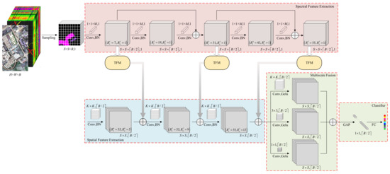
Figure 1.
Framework of the proposed LMFN for HSI classification. The upper line shows spectral correlation learning and the lower line concentrates on spatial dependence mapping. TFM blocks are the object-guided fusion mechanism used for spectral–spatial interactions.
The rest of this paper is organized as follows: We demonstrate our motivation by introducing the traditional 3D-CNN, then detail the proposed lightweight convolution factorization and target-guided fusion mechanism in Section 2. Section 3 reports the network configuration, experimental results, and corresponding discussions. Section 4 provides some conclusions.
2. Methodology
In this section, we first present the strengths and weaknesses of 3D-CNN in HSI feature learning. Thereafter, the proposed LMFN is detailed in two parts: The lightweight network architecture for multilevel feature learning and multiscale spectral–spatial interaction with the target-guided fusion mechanism.
2.1. Outline of the 3D-CNN for HSI Feature Learning
According to the combination of imaging and spectral technology, hyperspectral data are saved as a 3D digital cube, denoted as a tensor , with spatial size and spectral band number B (which is generally greater than one hundred). Its extremely high resolution prompts the spectrum to be better for mining the physical properties of ground objects, allowing for more accurate recognition. However, high-resolution image acquisition systems tend to corrupt the data with lots of noise, leaving the HSI with high-order non-linearity. Deep neural networks have excellent ability to approximate complex functions, especially CNNs for image data tasks. The 2D-CNN, with outstanding advantages in high-level spatial feature learning, has been widely used for natural image recognition purposes. Spectral information has received less attention, in relation to the 2D-CNN. This is principally attributed to the use of digital color images with only red, green, and blue channels, which provides a limited contribution to object recognition. The high-resolution spectra present in HSIs have led to new proposals, as well as new challenges, in ground object recognition.
In a standard 2D-CNN, as seen in Figure 2a, convolution kernels with a kernel size of perform one-on-one Multiply–Add operations on input channels in in a sliding-window manner, from top left to bottom right (⊗ indicates this operation), and with a default protocol where is equal to the input size . The obtained output slices are then accumulated to produce one feature map . The 2D-CNN focuses on spatial local perception and feature recombination, but pays less attention to spectral local perception. This processing can easily result in spectral information loss when compressing all of the convolutional results into one presentation for the subsequent layer, and the global perception on the spectral domain ignores the local dependence, which is relatively stronger than the spatial dependence used in HSIs. In order to focus on spectral–spatial multiscale perception simultaneously and equally, a 3D-CNN is a better choice. Different from the 2D-CNN, the 3D-CNN performs local convolution in three directions (as seen in Figure 2b) with kernel , which adds another dimension to and . The difference in kernel size brings distinct compositions to the input and output , where all channels are 3D tensors, but not 2D matrices. Figure 2b shows the case of a single channel (i.e., ). From the different operations, the 3D-CNN has significantly increased parameter counts and computational cost, compared with the 2D-CNN; for example, it has M times more parameters when set with the same input–output channels and ignoring the offsets. A similar situation occurs for CIO and FLOPs, where 3D-CNN increases the communication cost by times when setting the padding process for all convolution operations. Its computational cost is times that of the 2D-CNN.
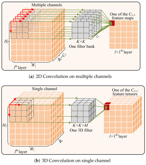
Figure 2.
Schematic illustration of 2D and 3D convolution.
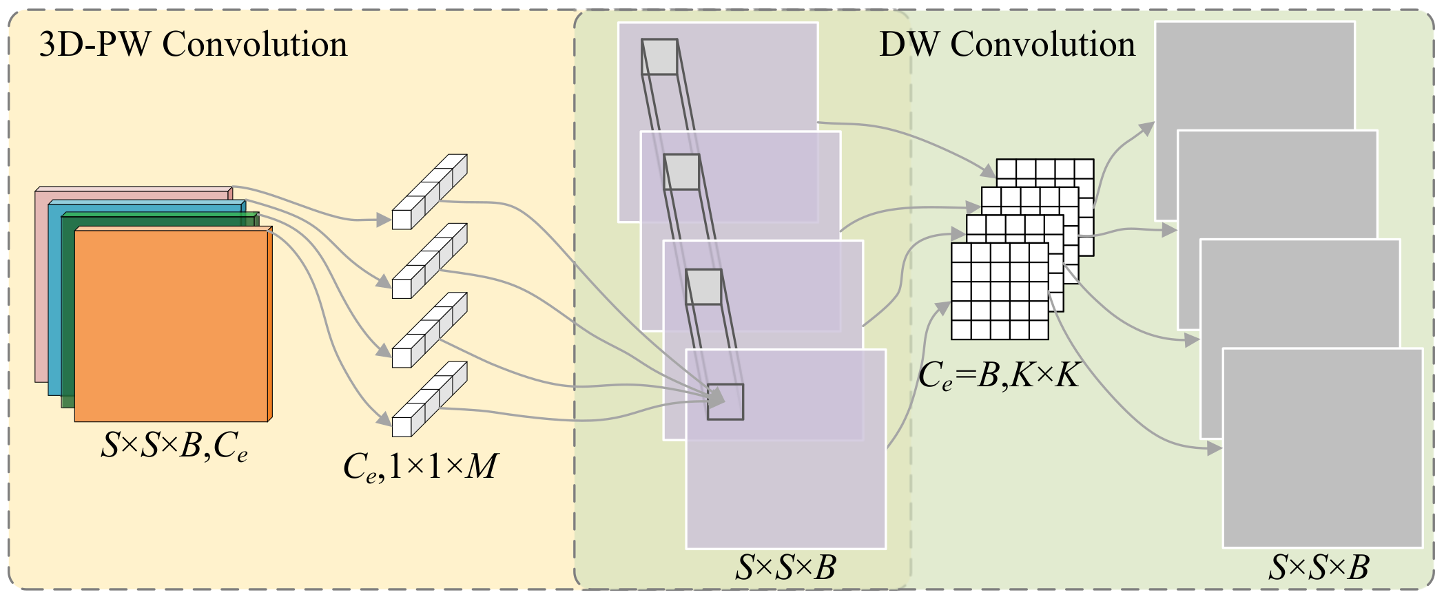
Depth-wise separable convolution factorizes the traditional 2D-CNN into two parts: depth-wise convolution (DW) and point-wise convolution (PW). This factorization drastically reduces the number of parameters and computational burden of 2D-CNNs, while maintaining almost the same feature learning effect [33]. Decoupling 3D-CNN in the same way although could decrease training parameters and FLOPs, the already large CIO will be doubled. For lightweight 3D spectral–spatial convolution, we separate the 3D-CNN into successive 3D point-wise convolution (PW) and 2D depth-wise convolution (DW), as seen in Figure 3. We aimed to discover multiscale local correlations among the spatial and spectral spaces in the HSI simultaneously and learn discriminative features, while having fewer possible parameters and less computation.

Figure 3.
Schematic illustration of lightweight 3D spectral–spatial feature learning with two parts: 3D-PW and DW convolution.
2.2. Lightweight 3D Convolution for Spectral–Spatial Feature Learning
Due to the extremely limited number of HSIs for training deep segmentation models, object recognition in HSIs is usually seen as a pixel-wise classification task. Thus, a 3D patch with a spatial size of and N neighboring pixels is split out as an input, in order to help in identifying the center pixel on the basis of the neighborhood consistency assumption and auxiliary spatial information. For lightweight multiscale perception from the spectral and spatial domains, we separate spectral–spatial feature extraction into two modules—spectral correlation learning (top line in Figure 1) and spatial feature mapping (bottom line)—in an end-to-end manner.
In the spectral feature extraction module, 3D filters are introduced to perform the convolution operation, where the depth M is less than the band number B. This is called 3D-PW. Deep CNNs abstract and conceptualize object representation by combining features from shallow textures to deep semantic information, where an important concept is the receptive field. To extract higher-order semantic information from the spectrum, we use five 3D-PW layers for neighborhood relationship mining with a gradual increase in the receptive field. All convolutions are set with the same kernel size and slide with stride 1; except for the first layer, which has stride 2 for dimension reduction. Figure 1 shows the receptive field size of each layer as and , where is the size of the spectral dimension and is the spatial receptive field. In the spectral module, the value of remains unchanged from 1, as none of the spatial neighborhood perception is presented here. In consideration of the relatively simple local directional information in the spectrum, and to achieve a more lightweight network, only one 3D kernel is used in each 3D-PW layer, which means , and the output has the same size () when the paddings are set for all convolutions. Experiments showed that including more 3D filters in each layer does not contribute to a greater classification accuracy. To alleviate the “Distortion” in the original spectral information during feature composition, and to prevent model degradation as the network deepens, we added shortcut connections between layers to aggregate low-level features from the feed-forward network to high-level layers, ensuring the deep layer has more (or, at least, no less) image information than the shallow one. Additionally, batch normalization (BN) follows each 3D-PW convolution, in order to enhance the generalizability and convergence behavior of the model. For further details about the settings, please see Figure 1.
In the spatial correlation learning module with lightweight architecture, we exclusively focused on each feature map but left channel correlations to the preceding spectral module. Thus, DW convolution was introduced to extract spatial features. Unlike the 2D-CNN, which produces a new representation by grouping features from the previous layer, DW applies a single convolutional kernel specifically to each input channel (as seen in Figure 3), and produces one corresponding feature representation in the th layer. To ensure that the spatial module possesses a large spectral receptive field for multiscale fusion, the spatial module is followed by the foregoing spectral module. With the originally limited spatial neighborhood in the input patch, there are only three DW layers for layer-wise perception and padding is set for all convolutions. In the spatial module, the value of remains unchanged as the last 3D-PW layer, as none of the channel neighborhood perception is presented here, but the spatial receptive field is enlarged along with the layer-wise DW convolution.
With this decomposition, our network backbone is much more lightweight. For comparison with the 3D-CNN on an equal basis, we carried out once-through spectral–spatial convolution with one 3D-PW spectral module and one DW spatial module (as illustrated in Figure 3), with the same filter size as detailed in Section 2.1. This combined block produced the following number of parameters:
where M represents the 3D-PW convolution and represents the DW convolution. The computational cost was
FLOPs, in total. Both indicators had lower values than the original depth-wise separable convolution, which can mainly be attributed to the use of only one 3D filter in the 3D-PW for local spectral recombination. Our decoupled spectral–spatial convolution achieved a much better effect than the standard 3D-CNN, even when we set the 3D-PW part with the same filter bank. More specifically, our proposed model produced about the parameters and the computational cost of the 3D-CNN. Factorization of 3D-CNN into 3D-PW and DW caused our method to require twice the communication cost for the CIO, compared with the standard 2D-CNN, but this increase is acceptable, compared with the traditional 3D-CNN ( times that of 2D-CNN).
2.3. Target-Guided Fusion Mechanism
The separation of the spectral and spatial modules can easily lead to information loss as the network deepens, especially when spatial filtering follows the spectral module. Meanwhile, the large size of the spectral-spatial receptive field at the end of the network framework causes the feature to be insensitive to local finer perception. Moreover, DW convolution filters each input feature map independently, giving fast response and performance, but it tends to break the correlations between channels. Direct addition of the foregoing multiscale spectral features which with the smallest spatial receptive field, to the depth-wise spatial module, can compensate for the problem mentioned above. However, the intact spatial adjacent relationship may cause irrelevant information and especially the noise flow into the deep layers. A target-guided fusion mechanism (TFM), therefore, is proposed to enhance adjacent spectral correction and focus on pixels which actively boost the target classification accuracy, while performing multiscale feature fusion. The primary line is formulated as
where denotes the calculated target-based response from one feature bank in the spectral module, and is a feature tensor from the spatial convolution module. The spectral module contains features with incremental receptive fields in the spectral domain but with unaltered neighborhood perception in the spatial domain, while the spatial module has the reverse situation. Thus, we added sequentially to the spatial module to achieve spectral–spatial fusion. is the obtained multiscale feature from one set of spectral–spatial features.
As mentioned earlier, a block of neighborhood members around the center pixel are split out to assist with target classification. These neighbors inevitably contain some pixels unrelated to the center target, particularly for ground surface objects with limited contributions to high-level outlines. This means that not all the neighborhood information has a positive effect on network performance improvement. Hence, before feature fusion, pairwise-dependent relationships are built between and its neighborhood in from the spectral layer, and the tensor is produced to guide spatial convolution, paying close attention to areas that should be of concern. This is formulated as:
where is the set of N neighbors () around , and is the output of TFM, with the same size as , to be fused. The function measures the correlation between and : the larger the value, the higher the correlation and, thus, the greater the influence of the weight on the center point. We chose the Cosine distance to measure the similarity. The target-guided fusion mechanism can be seen as a 2D convolution on (as seen in Figure 4), and the kernel is generated by the feature at the input center; that is, . Then, TFM can be formulated as:
where ⊗ and ⊙ indicate 2D convolution and scalar multiplication, respectively. The sigmoid function is designed here with two main considerations: (1) It can compress the obtained similarity value into , in order to produce a controllable weighting coefficient; (2) it will heighten the areas of attention by stretching the two extreme values (positive or negative) to the saturated zone, thus preventing further noise passing through when information flows from the previous layers.
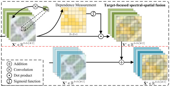
Figure 4.
Schematic illustration of the object-guided spectral–spatial fusion mechanism (TFM).
We can conclude that one TFM block increases CIO and FLOPs from the dependence measurement and point-wise multiplication, and has about the communication cost and the computational cost of the 3D-CNN, on the basis of the previous analysis.
The 3D-PW and DW convolution operations can be regarded as feature mapping in spectral and spatial spaces independently, while the TFM is responsible for interaction and circulation of the information, with clear division of the two. As little burden is produced, in terms of parameters storage and computational cost, we present three TFMs on the end of each identity residual block for long range skip-connection and multiscale spectral–spatial fusion, as shown in Figure 1. After the 3D interactive feature learning, a multi-scale filter bank (with kernel size of , , ) and GELU activation are introduced for local multi-level convolution of the input feature, using filters to address channel correlations. Finally, a global average pooling (GAP) and fully connected (FC) layer are introduced for probability prediction of object classification.
3. Experiments and Discussion
In this section, we evaluate the LMFN against three public HSI benchmark data sets through a parameter analysis and performance comparison with several recent state-of-the-art approaches.
3.1. Data Description
The Indian Pines (IN) data set was collected by the Airborne Visible/Infrared Imaging Spectrometer (AVIRIS) sensor over the agricultural Indian Pine test site in northwestern Indiana in 1992. The IN contains 200 spectral bands (after removing 20 noisy bands) with wavelengths ranging from 0.2 to 2.4 m and image size of 145 × 145 pixels with a spatial resolution of 20 m/pixel. This data set has a greater number of spectral bands but more noise disturbance in the experimental data. Sixteen different objects with 10,249 pixels in total are labeled in this data set. Figure 5 shows its false-color images and the corresponding ground-truth, respectively.
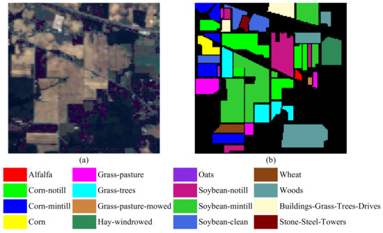
Figure 5.
(a) False-color image and (b) ground truth for the IN data set.
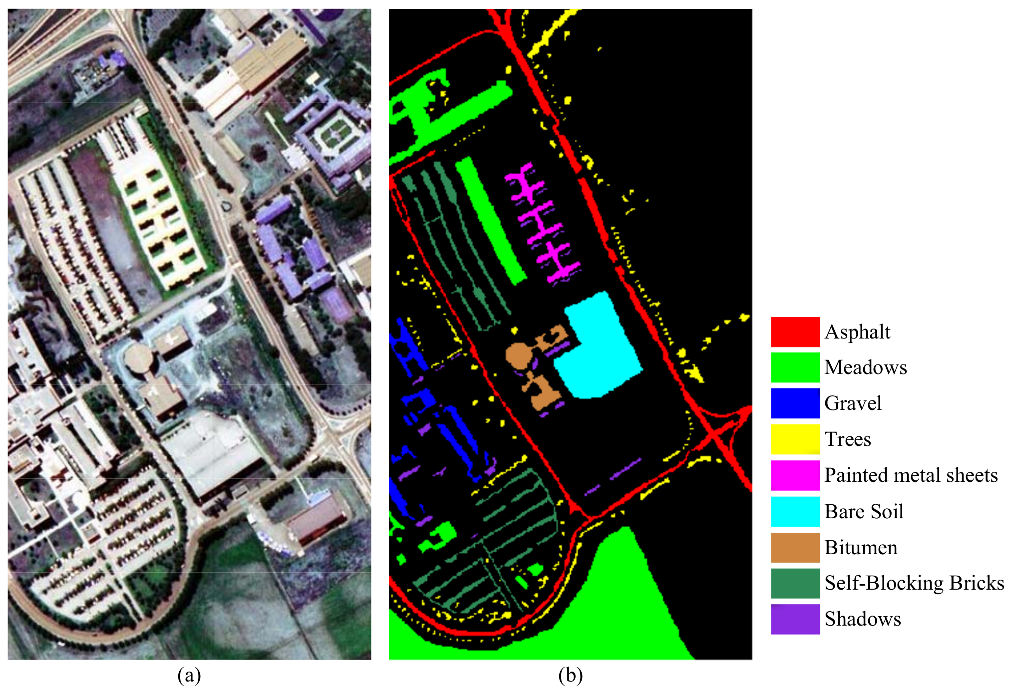
The University of Pavia (UP) data set was acquired by the Reflective Optics System Imaging Spectrometer (ROSIS) sensor over the university campus in Pavia, Northern Italy in 2001. The UP has 103 spectral bands (after removing 12 noisy bands), with wavelengths ranging from 0.43 to 0.86 m and image size of 610 × 340 pixels with a spatial resolution of 1.3 m/pixel. This data set contains nine labeled classes with a total of 42,776 pixels, and it has an abundant spatial structure. Figure 6 shows its false-color images and the corresponding ground-truth, respectively.

Figure 6.
(a) False-color image and (b) ground truth for the UP data set.
The KSC data set was collected by AVIRIS in Florida in 1996. This data set contains images with size of 512 × 614 pixels, with a spatial resolution of 18 m/pixel and 13 labeled classes in the ground-truth. After removing the noisy bands, 176 spectral features were retained for ground object recognition in our experiments. Figure 7 shows the false-color image and corresponding ground-truth for this data set.
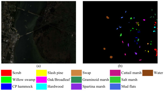
Figure 7.
(a) False-color image and (b) ground truth for the KSC data set.
3.2. Experimental Settings
During the course of implementing LMFN, we employed the cross-entropy loss method for category prediction and stochastic gradient descent (SGD) to update the model parameters. We used an initial learning rate of 0.01, a weight decay of 0.0001, and a momentum of 0.9. In particular, when the loss updating ground to a halt, we reduced the learning rate to one-half of its current state. Through experimental observations, we set all training epochs to 100 and batch sizes to 32 for the IN, UP, and KSC data sets.
In relation to the experimental data sets with uneven scales, different proportions of labeled samples in each HSI were allocated to the training and testing sets for model optimization and performance evaluation. Specifically, we randomly selected 10%, 3%, and 5% of the labeled samples in the IN, UP, and KSC data sets for model training, respectively, and the other 90%, 97%, and 95% of labeled samples were used for testing. Before model training, the original HSI data were first standardized and mapped to for dimensionless transformation in each spectral band. The overall accuracy (OA), average accuracy (AA), and kappa coefficient (Kappa) were used as quantifiable indicators to validate the classification performance. All results are reported as the mean and standard deviation of ten runs, and we provide OA plots as a function of the parameters to be analyzed. All experiments were performed on a machine equipped with an Intel Xeon W-2133 CPU and an NVIDIA GeForce RTX 2080Ti graphics card. The experimental software environments used were Python 3.8.3, PyTorch 1.7.0, and CUDA 11.0. Code is available at: https://github.com/JXUST-HyperSpectralImage/LMFN.git (accessed on 13 December 2021).
3.3. Parameter Analysis
In our proposed LMFN, the main parameters influencing model performance are the input patch size for neighborhood information assistance, the kernel size in the 3D-PW module for spectral feature extraction, and the number of TFM blocks for spectral–spatial interactions. To better show the details of the proposed model, an example with specific parameters is shown in Table 1, where the input data are a 3D cube of size ().

Table 1.
Implementation details for an example of the LMFN.
3.3.1. Influence of the Input Patch Size
As described in Section 2.2, a 3D patch centered with object pixels is split out as the input of LMFN for spectral–spatial feature learning. Generally, with a larger input patch size S, more spatial information is included to assist in classification; however, this increases the computational burden. Additionally, we cannot ensure that all neighborhoods with a wide range can play a positive role in promoting classification accuracy.
Before analyzing this parameter, we set the 3D-PW convolutional kernel size and TFM block number to and 3, respectively, for all HSI data sets. Table 2 shows the OA results when the patch size was an odd number ranging from 5 to 13. We can see that the classification accuracy of both IN and UP increased and then became stable when S was larger than . A different situation occurred for the KSC data set: the accuracy reached a peak when , but began to decline after that. This may be attributed to the smaller land area that the objects covered in the KSC, and neighborhoods in over-large patches may have disturbed center object recognition. To balance the classification precision and computational cost, we set the patch size to . Thus, was the input of the LMFN for all experimental data sets.
Table 2.
Classification performance of all three data sets with the input patch size of the LMFN ranging from to , in terms of OA (%). The best results are highlighted in bold font.
3.3.2. Influence of the Kernel Size in the 3D-PW
In our LMFN, for HSI classification, we focused more on spectral feature learning. Thus, 3D-PW convolutions were proposed for filtering purely in the spectral dimension, and the 3D filter was defined as in Section 2.2. The parameter setting of M may affect the model’s performance in terms of feature learning, especially when the HSI data sets were obtained using different sensors, leading to diverse spectral resolutions.
We evaluated the influence of the kernel size when M ranged from 5 to 13 with the patch size set to and the TFM block number set to 3 for all the data sets. Table 3 shows the OA results as a function of the kernel size . We observed that the performance of the proposed LMFN gradually improved as the value of M increased for IN, while the OA results appear to be relatively stable for the UP and KSC data sets. This may indicate that our model—especially the TFM, as a self-supervised block in multiscale feature learning—is robust against the convolutional kernel size, which is desirable in deep learning-based methods. To balance between classification accuracy and parameter number, we set the kernel size in the 3D-PW convolution to for all experiments, producing a filter bank that contains very few parameters for training.
Table 3.
Results for all three experimental data sets, in terms of OA (%), as a function of kernel size in 3D point-wise convolution. The best results are highlighted in bold font.
3.3.3. Influence of the TFM Block Number
The TFM is an important component of our proposed LMFN. It is a block for center target-focused supervised learning and spectral–spatial interaction. Thus, the more TFM blocks introduced to LMFN, the better the feature learning performance. The experimental results reported in Table 4 further indicate this as the TFM number gradually increased from the deep to shallow layers: “0” indicates that the TFM was not introduced into the backbone lightweight network, while “3” indicates that three TFM blocks were added (see Figure 1). Both of the other parameters were set as before.
Table 4.
Classification performance of the three data sets, considering the TFM number in the backbone lightweight framework ranging from 0 to 3 and comparison with a fusion mechanism of NoT-FM in terms of the OA (%). The best results are highlighted in bold font.
The results show that the classification accuracy had a comparatively large improvement when the TFM block started from scratch, and the results tended to be stable (as the number was greater than 1); except for the KSC, which showed a slightly larger enhancement. This demonstrates that features from the deep layer are more important for the recognition of ground-objects trapped in a highly non-linear distribution, and multi-scale fusion gives the network better performance. The introduction of the TFM block only increases the number of training parameters and computational cost by small amounts; thus, we added three TFMs on the end of all the identity residual blocks for spectral–spatial interaction.
To confirm the effectiveness of TFM in feature fusion, we further compared it with a fusion mechanism which adds directly to without object guidance (NoT-FM for short). From the OA results of classification as in Table 4, we can find that TFM performs uniformly better than NoT-FM, whether with one connection in the deep layer or three numbers of multiscale fusion from deep to shallow layers. Furthermore, more notably, NoT-FM made the results even worse than no spectral–spatial fusion between the two modules in the IN data set. That is probably because the noise was enlarged and flowed from the shallow to the deep layers and thus it disrupted the contextual perception in the spatial module. Our proposed TFM can avoid this problem by target guidance. We added these experimental results and analyses in our new manuscript.
3.4. Comparison with State-of-the-Art Methods
We compared our proposed LMFN with some state-of-the-art methods for a validity analysis. In consideration of the 3D convolution, spectral–spatial fusion, residual connection, and multiscale fusion strategies adopted in our deep model, we employed CDCNN [22], 3DCNN [34], SSRN [26], DFFN [24], and MFDN [27] for comparison, which contain these components to varying degrees, while SVM was used as the baseline. More specifically, the CDCNN uses multiscale 2D filters in the initial layer, followed by two residual blocks for spectral feature learning. The 3DCNN can process spectral and spatial information simultaneously with a lower computational cost. The SSRN first extracts spectral features by 3D convolution, followed by 2D convolution for spatial feature learning. Additionally, residual connections are introduced in both parts. The MFDN extracts spectral and spatial information in a similar manner to the SSRN, except that PCA dimensional reduction is introduced before spatial learning, and both parts have a parallel framework. Finally, the learned spectral and spatial features are concatenated together for feature fusion using a 3D dense convolution block. DFFN is an exclusive 2D-CNN network with residual learning that performs feature extraction on the spatial dimension after PCA processing, and multiple level features from each residual block are summed and fused together for HSI classification. In addition, in consideration of the light and self-attention processing in our model, recent publications that studied the attention mechanism and parameter reduction were also considered for comparison here. More precisely, we took into account the following methods: CBW [35], FGSSCA [36], LDN [31], S2FEF-CNN [29], and S3EResBoF [30]. The CBW is a novel plug-and-play compact band weighting (CBW) module—a lightweight module with only 20 parameters—which can evaluate spectral band weighting by adjacent correlations and recalibrate HSIs for further feature learning. The FGSSCA integrates a spectral attention module and a spatial attention module by pooling information squeeze operations, in order to provide the same level of information recalibration. Then, the generated HSIs are grouped to learn spatial–spectral features separately. The LDN is a two-branch, lightweight deep network that decomposes a standard 3D convolution into a 3D group convolution and point-wise convolution to reduce the number of parameters. The S2FEF-CNN is a lightweight network where each S2FEF block uses 1D convolution to extract spectral features and 2D convolution to extract spatial features, respectively, and then fuses the obtained features by multiplication. The S3EResBoF does not lightweight the deep model from convolution operations but replaces the general pooling method with bag of features [30] to reduce the parameters in the fully connected layer.
In the experimental implementation, the SVM parameters obtained through five-fold cross-validation, and parameters in all other comparison methods were set as given in the corresponding references. All comparative deep-learning-based methods set individual network parameters for different data sets; thus, we determined parameter settings through experiments and referred to the existing data for the experimental data sets that were not shared. For our LMFN, as previously analyzed, we set the same parameters for all data sets, where was the input, the kernel size in 3D-PW convolution was , and three TFM blocks were added to the deep model. For fair comparison, we used the same number of randomly selected samples for the optimization of all models, as described in Section 3.2. All experimental results were averaged after repeating each method ten times.
3.4.1. Comparison of Parameter Numbers and Computation Efficiency
The main purpose of this paper was to design a lightweight network. Thus, we first summarized the parameter storage, computational cost, and communication cost of each method, as presented in Table 5, where FLOPs are reported for the computational cost, CIO values represent the communication cost, and the training time and testing time are reported in terms of the overall running consumption. All models were counted in the state of optimal accuracy and were trained with samples at the same scale. It can be seen that LMFN required the least number of parameters, and saved almost 98% in storage compared with the most heavy model, MFDN, within each group in the table; a similar situation was observed for FLOPs. LMFN was not the best in terms of CIO and, thus, was slightly more computationally time-consuming, but it was acceptable when compared with the least time-consuming method, especially when compared with the MFDN, which is competitive in terms of classification accuracy. One of the most competitive methods is the CBW, which presented an excellent performance for most of the indicators, except for having relatively more FLOPs. Nonetheless, the CBW was found to be relatively sensitive to data properties and unfavorable in terms of its general applicability, for which we will provide further explanation later. The three lightweight models, LDN [31], S2FEF-CNN [29], and S3EResBoF [30], although all contain a competitive number of parameters, need a large amount of the CIO and FLOPs, especially FLOPs of LDN is hundreds more than ours. Methods other than the CBW either achieved a relatively worse classification performance or gained a superior classification accuracy by sacrificing storage, computation, or communication. It is worth noting that our LMFN has a similar backbone to SSRN, but the lightweight processing and object-guided fusion mechanism provide the LMFN greater advantages, in terms of both storage and computing burden, with a more outstanding classification accuracy. As a whole, although our proposed LMFN did not perform the best for all indicators, it was comparable and reasonable, in terms of lightweight execution.
Table 5.
Comparison of running time, parameter number, FLOPs, and CIO of different deep models on three datasets. OAs are provided here for comprehensive performance evaluation. The best results are highlighted in bold font.
3.4.2. Classification Results
Classification results for the three data sets are reported in Table 6, Table 7 and Table 8. It can be observed that the MFDN performed better than the other comparative methods for the UP and KSC data sets, while the FGSSCA performed best on the IN data set. Our proposed LMFN was behind the best results by 1.22%, 1.92%, and 2.06%, respectively, in the OA results for the three data sets. The LMFN performed more consistently than the CDCNN, 3DCNN, SSRN, and the purely 2D convolution network DFFN. What is even more remarkable is that the 3DCNN achieved better classification accuracy than DFFN for the IN, but showed worse results on both the UP and KSC data sets. This is because the 3DCNN can focus and balance on both the spectral and spatial features, while the DFFN places emphasis on spatial filtering. Consequently, the 3DCNN, with fewer layers, performs better when the experimental data contain richer spectral information, but performs worse than the DFFN when the spatial structure facilitates better ground object identification. However, our method was compatible with both of these extremes. The network architecture of SSRN was similar to ours when no TFM block was added to the backbone; thus, it obtained pretty much the same results as the LMFN with no TFM in Table 4, but it required more parameters and had a greater computational burden. This further confirms the effectiveness of our proposed TFM block and lightweight LMFN.
Table 6.
Performance comparison with state-of-the-art methods, in terms of classification accuracy, for the IN data set. The best results are highlighted in bold font.
Table 7.
Performance comparison with state-of-the-art methods, in terms of classification accuracy, for the UP data set. The best results are highlighted in bold font.
Table 8.
Performance comparison with state-of-the-art methods, in terms of classification accuracy, for the KSC data set.The best results are highlighted in bold font.
Furthermore, our model was inferior to the MFDN on the UP and KSC data sets. This was because the MFDN also puts more emphasis on spectral information, where 3D dense convolutions with a kernel size of are introduced for spectral feature learning. Despite achieving the best results, this success, in terms of accuracy, called for many more parameters and a greater computational burden, as mentioned earlier. Significantly, the IN data set has more spectral bands but a worse spatial resolution, with strong noise and disturbances. At this point, our proposed TFM block performed better, in terms of noise suppression and spectral–spatial fusion. Compared with the attention mechanism network, the CBW performed better than our method on HSIs that contain objects with a wide spectrum difference, such as IN and UP, but performed worse when the ground objects had similar spectral information, such as the KSC, having an extensive marsh. Our LMFN behaved better, in this respect, which indicates that first-hand spectral learning with the 3D-PW could reduce information corruption, compared with the CBW, which extracts band correlations after spatial squeezing. The same situation presented for the FGSSCA further illustrates this point. In comparison with the lightweight model, the LDN and S3EResBoF perform slightly better than our model on IN and KSC datasets. This demonstrates that a deep network with a more complicated structure will be stronger in fitting high-order non-linear distribution. S2FEF-CNN requires a large number of training samples to optimize the parameters. Thus, it underperforms in classification accuracy in the small sample condition.
Figure 8, Figure 9 and Figure 10 show the corresponding visualization results for IN, UP, and KSC, respectively. As can be seen, our LMFN behaved better on the boundary, and was even superior to MFDN in some cases—for example, in the regions of “Self-Blocking Bricks” and “Bitumen” in the UP data. This may be ascribed to the input of the 2D spatial convolution module in MFDN, which has a larger patch size of , even though modules for spectral learning and feature fusion have made great advances. A similar, but worse, situation was presented for DFFN and LDN for all data sets; especially LDN, which was overly coarse even when an input patch size of was used. This may be due to the absence of a skip connection for information flow from shallow to deep layers in the LDN. In contrast, SSRN, CBW, FGSSCA, S2FEF, S3EResBoF, and our LMFN showed finer classification boundaries, which benefited from either multiscale information flow or from self-attention-based supervised learning. Furthermore, the SVM and CDCNN produced more noisy points in the classification maps. This is principally because SVM only uses spectral features for HSI classification, while the CDCNN mainly includes a convolution operation and does not pay adequate attention to spatial correlations. This demonstrated that it is not feasible to rely on spatial or spectral information alone for HSI classification, and both deserve significant attention.
3.4.3. Effectiveness with Limited Samples
We further validated the effectiveness of our proposed LMFN under the condition of limited training samples. Figure 11 exhibits all OA plots from the three experimental data sets, where the proportion of training samples ranged uniformly from 1% to 15%. It can be seen that, when more samples were used in model training, a greater classification accuracy was achieved for all methods. On average, the LMFN was second, in terms of overall accuracy, with the first position being given to MFDN or CBW. The LMFN performed a little worse, but gave comparable results to the CBW with the exception being when 1% of the training set was employed for model optimization on the IN. The cause of this problem may be that there was only one sample from four classes in the IN for model training at that level. Once these random samples are burdened with noise interference, feature fusion by the TFM block may prevent the right decision from being made. It is gratifying that this can be corrected rapidly by using slightly more training samples.
From the results on the UP data set, it can be observed that the LMFN placed third, in terms of overall accuracy. Additionally, our method fell behind the 2D spatial convolution network DFFN when the training samples were employed in a proportion of greater than 10%. This further demonstrates that our method gives slightly unfavorable results when the experimental data contain more spatial information but relatively fewer spectral bands. The depth-wise lightweight processing, indeed, prevents the recombination of spatial information between channels in each layer, which allows it to be lightweight, but has a certain expense in terms of classification accuracy. When compared with the lightweight methods, the LMFN performed close to the S3EResBoF on the UP and KSC data sets and was better than LDN and S2FEF on the IN and UP data sets, in terms of accuracy. Although the MFDN had the best classification performance on the KSC if we overlook its computational burden, it is noteworthy that our LMFN was competitive with CBW and FGSSCA, two feature squeeze-based self-attention methods, especially under the conditions of having limited training samples. In short, our proposed LMFN was stable and adaptable to all data sets, and its classification performance was comparable, although it was not the best.
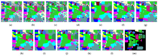
Figure 8.
Classification maps for the IN data set obtained by (a) SVM, (b) CDCNN, (c) 3DCNN, (d) SSRN, (e) DFFN, (f) MFDN, (g) CBW, (h) FGSSCA, (i) LDN, (j) S2FEF, (k) S3EResBoF, (l) LMFN, and (m) Ground truth.
Figure 8.
Classification maps for the IN data set obtained by (a) SVM, (b) CDCNN, (c) 3DCNN, (d) SSRN, (e) DFFN, (f) MFDN, (g) CBW, (h) FGSSCA, (i) LDN, (j) S2FEF, (k) S3EResBoF, (l) LMFN, and (m) Ground truth.
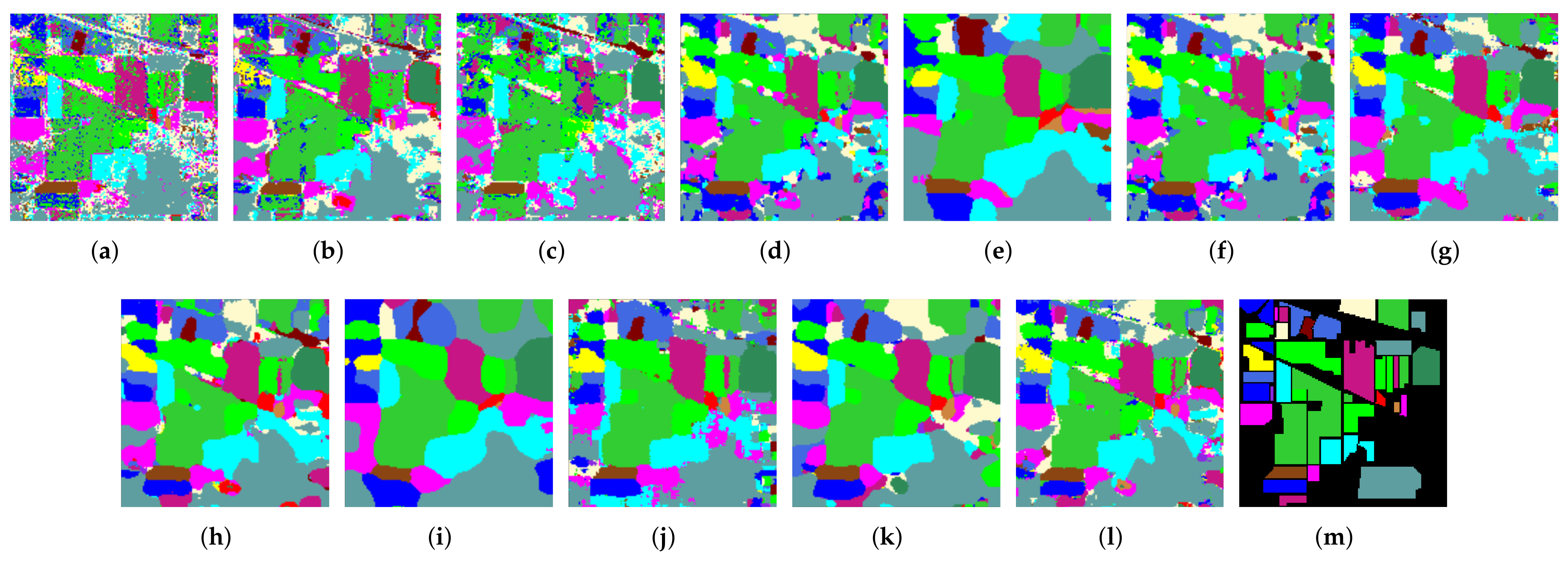

Figure 9.
Classification maps for the UP data set obtained by (a) SVM, (b) CDCNN, (c) 3DCNN, (d) SSRN, (e) DFFN, (f) MFDN, (g) CBW, (h) FGSSCA, (i) LDN, (j) S2FEF, (k) S3EResBoF, (l) LMFN, and (m) Ground truth.
Figure 9.
Classification maps for the UP data set obtained by (a) SVM, (b) CDCNN, (c) 3DCNN, (d) SSRN, (e) DFFN, (f) MFDN, (g) CBW, (h) FGSSCA, (i) LDN, (j) S2FEF, (k) S3EResBoF, (l) LMFN, and (m) Ground truth.
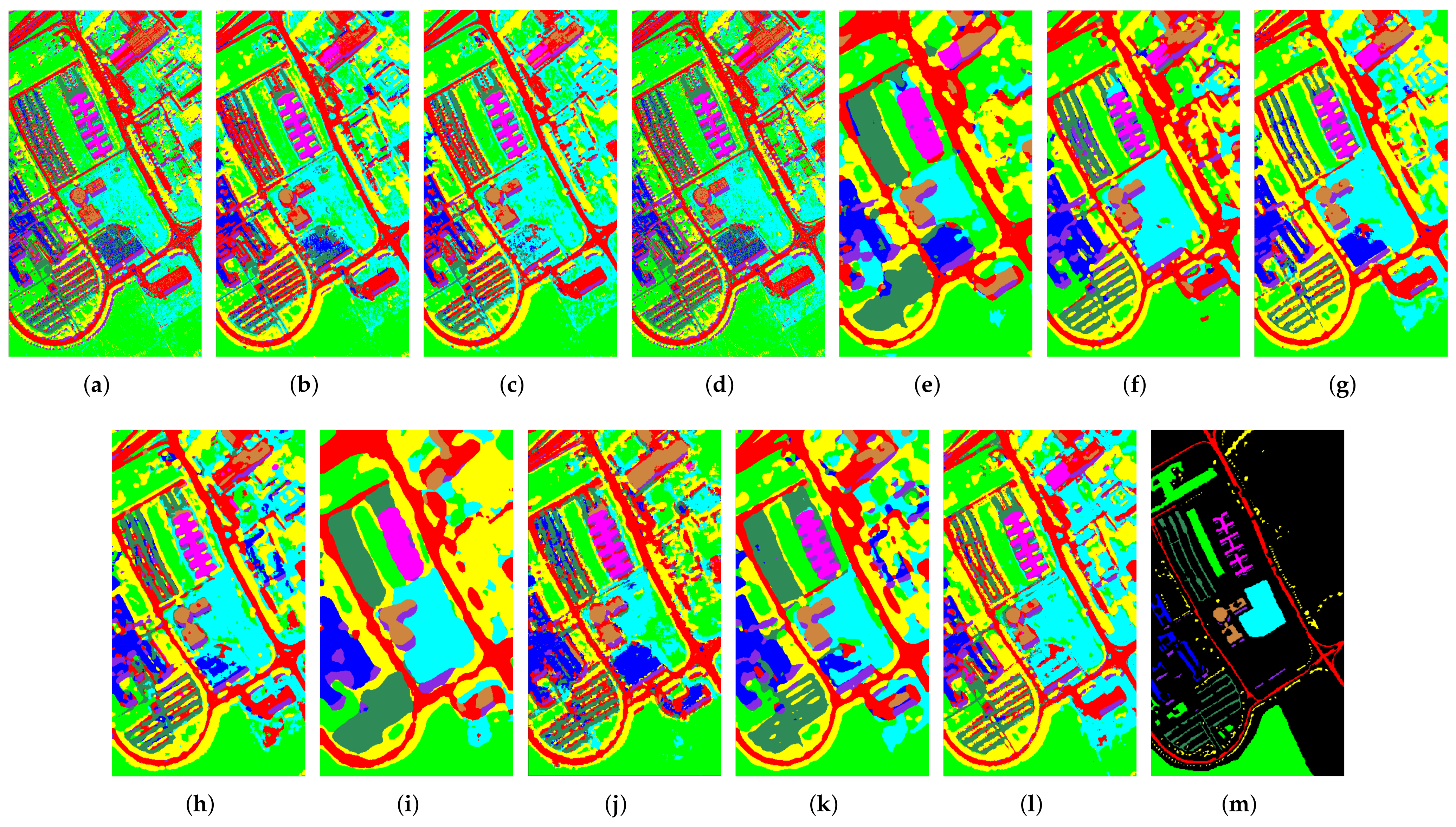
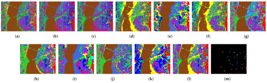
Figure 10.
Classification maps for the KSC data set obtained by: (a) SVM, (b) CDCNN, (c) 3DCNN, (d) SSRN, (e) DFFN, (f) MFDN, (g) CBW, (h) FGSSCA, (i) LDN, (j) S2FEF, (k) S3EResBoF, (l) LMFN, and (m) Ground truth.
Figure 10.
Classification maps for the KSC data set obtained by: (a) SVM, (b) CDCNN, (c) 3DCNN, (d) SSRN, (e) DFFN, (f) MFDN, (g) CBW, (h) FGSSCA, (i) LDN, (j) S2FEF, (k) S3EResBoF, (l) LMFN, and (m) Ground truth.
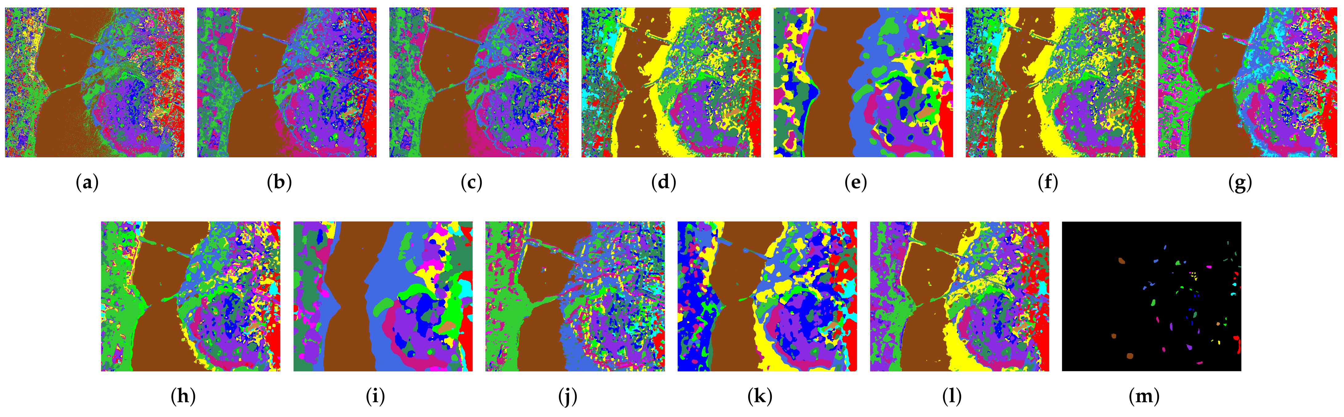
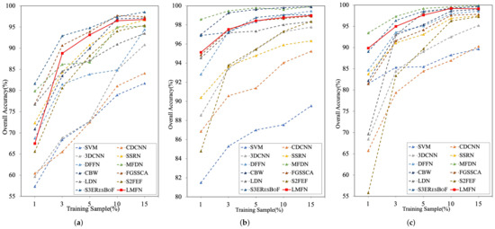
Figure 11.
OA results of all the compared methods with varying proportions of training samples (from 1 to 15%) on the (a) IN, (b) UP, and (c) KSC data sets.
Figure 11.
OA results of all the compared methods with varying proportions of training samples (from 1 to 15%) on the (a) IN, (b) UP, and (c) KSC data sets.
4. Conclusions
In this paper, we introduced a lightweight deep learning framework with a target-guided fusion mechanism for HSI classification. The proposed LMFN decouples the standard 3D convolution into successive 3D-PW convolution and 2D-DW convolution for specific spectral and spatial feature learning, respectively. Meanwhile, the target-guided fusion mechanism was proposed as a bridge for spectral–spatial interaction among the two separate modules. This center-pixel-guided method, while in multiscale feature fusion, enhanced adjacent spectral correction and spatial attention. Experimental results across three public HSI benchmark data sets demonstrated that the LMFN has a competitive advantage, in terms of both classification accuracy and lightweight deep network architecture engineering, with a certain level of robustness and adaptability. This performance evaluation indicated that the spectral and spatial information in HSIs both deserve significant attention when carrying out ground–object recognition.
In the future, we will focus on discovering a lightweight but adaptive dynamic convolution network with more robust attention mechanism that is suited to HSI feature learning and classification.
Author Contributions
Conceptualization, H.W. and M.L.; methodology, H.W. and M.L.; software, H.W.; validation, H.W. and X.Y.; formal analysis, H.W. and M.L.; investigation, H.W. and J.Y.; resources, M.L.; data curation, H.W. and Z.M.; writing—original draft preparation, H.W.; writing—review and editing, M.L. and X.Y.; visualization, H.W.; supervision, L.J.; project administration, M.L.; funding acquisition, M.L. All authors have read and agreed to the published version of the manuscript.
Funding
This research was funded by the National Natural Science Foundation of China of FUNDER under grant numbers 61901198 and 61862031, the Natural Science Foundation of Jiangxi Province of FUNDER under grant number 20181BAB202004, and the Program of Qingjiang Excellent Young Talents, Jiangxi University of Science and Technology of FUNDER under grant number JXUSTQJYX2020019.
Institutional Review Board Statement
Not applicable.
Informed Consent Statement
Not applicable.
Data Availability Statement
Data presented in this study are available at: http://www.ehu.eus/ccwintco/index.php?title=Hyperspectral_Remote_Sensing_Scenes, accessed on 13 December 2021.
Conflicts of Interest
The authors declare no conflict of interest.
Abbreviations
The following abbreviations are used in this manuscript:
| MDPI | Multidisciplinary Digital Publishing Institute |
| DOAJ | Directory of open access journals |
| TLA | Three letter acronym |
| LD | Linear dichroism |
References
- Zhang, L.; Zhang, L.; Du, B. Deep learning for remote sensing data: A technical tutorial on the state of the art. IEEE Geosci. Remote Sens. Mag. 2016, 4, 22–40. [Google Scholar] [CrossRef]
- Tian, A.; Fu, C.; Yau, H.T.; Su, X.Y.; Xiong, H. A New Methodology of Soil Salinization Degree Classification by Probability Neural Network Model Based on Centroid of Fractional Lorenz Chaos Self-Synchronization Error Dynamics. IEEE Trans. Geosci. Remote Sens. 2019, 58, 799–810. [Google Scholar] [CrossRef]
- Yang, X.; Yu, Y. Estimating soil salinity under various moisture conditions: An experimental study. IEEE Trans. Geosci. Remote Sens. 2017, 55, 2525–2533. [Google Scholar] [CrossRef]
- Zhong, Y.; Wang, X.; Xu, Y.; Wang, S.; Jia, T.; Hu, X.; Zhao, J.; Wei, L.; Zhang, L. Mini-UAV-borne hyperspectral remote sensing: From observation and processing to applications. IEEE Geosci. Remote Sens. Mag. 2018, 6, 46–62. [Google Scholar] [CrossRef]
- Liu, Q.; Xiang, X.; Yang, Z.; Hu, Y.; Hong, Y. Arbitrary Direction Ship Detection in Remote-Sensing Images Based on Multitask Learning and Multiregion Feature Fusion. IEEE Trans. Geosci. Remote Sens. 2020, 59, 1553–1564. [Google Scholar] [CrossRef]
- Bioucas-Dias, J.M.; Plaza, A.; Camps-Valls, G.; Scheunders, P.; Nasrabadi, N.; Chanussot, J. Hyperspectral remote sensing data analysis and future challenges. IEEE Geosci. Remote Sens. Mag. 2013, 1, 6–36. [Google Scholar] [CrossRef] [Green Version]
- Bandos, T.V.; Bruzzone, L.; Camps-Valls, G. Classification of hyperspectral images with regularized linear discriminant analysis. IEEE Trans. Geosci. Remote Sens. 2009, 47, 862–873. [Google Scholar] [CrossRef]
- Xia, J.; Chanussot, J.; Du, P.; He, X. Rotation-Based Support Vector Machine Ensemble in Classification of Hyperspectral Data With Limited Training Samples. IEEE Trans. Geosci. Remote Sens. 2015, 54, 1519–1531. [Google Scholar] [CrossRef]
- Li, J.; Bioucas-Dias, J.M.; Plaza, A. Semisupervised Hyperspectral Image Segmentation Using Multinomial Logistic Regression With Active Learning. IEEE Trans. Geosci. Remote Sens. 2010, 48, 4085–4098. [Google Scholar] [CrossRef] [Green Version]
- Yang, J.; Kuo, B.; Yu, P.; Chuang, C. A Dynamic Subspace Method for Hyperspectral Image Classification. IEEE Trans. Geosci. Remote Sens. 2010, 48, 2840–2853. [Google Scholar] [CrossRef]
- Du, B.; Zhang, L. Random-Selection-Based Anomaly Detector for Hyperspectral Imagery. IEEE Trans. Geosci. Remote Sens. 2011, 49, 1578–1589. [Google Scholar] [CrossRef]
- Li, S.; Song, W.; Fang, L.; Chen, Y.; Ghamisi, P.; Benediktsson, J.A. Deep Learning for Hyperspectral Image Classification: An Overview. IEEE Trans. Geosci. Remote Sens. 2019, 57, 6690–6709. [Google Scholar] [CrossRef] [Green Version]
- Tao, C.; Pan, H.; Li, Y.; Zou, Z. Unsupervised Spectral–Spatial Feature Learning With Stacked Sparse Autoencoder for Hyperspectral Imagery Classification. IEEE Geosci. Remote Sens. Lett. 2015, 12, 2438–2442. [Google Scholar] [CrossRef]
- Chen, Y.; Lin, Z.; Zhao, X.; Wang, G.; Gu, Y. Deep Learning-Based Classification of Hyperspectral Data. IEEE J. Sel. Top. Appl. Earth Observ. Remote Sens. 2014, 7, 2094–2107. [Google Scholar] [CrossRef]
- Zhou, P.; Han, J.; Cheng, G.; Zhang, B. Learning Compact and Discriminative Stacked Autoencoder for Hyperspectral Image Classification. IEEE Trans. Geosci. Remote Sens. 2019, 57, 4823–4833. [Google Scholar] [CrossRef]
- Chen, Y.; Zhao, X.; Jia, X. Spectral–spatial classification of hyperspectral data based on deep belief network. IEEE J. Sel. Top. Appl. Earth Observ. Remote Sens. 2015, 8, 2381–2392. [Google Scholar] [CrossRef]
- Chen, Y.; Jiang, H.; Li, C.; Jia, X.; Ghamisi, P. Deep Feature Extraction and Classification of Hyperspectral Images Based on Convolutional Neural Networks. IEEE Trans. Geosci. Remote Sens. 2016, 54, 6232–6251. [Google Scholar] [CrossRef] [Green Version]
- Yang, J.; Zhao, Y.Q.; Chan, C.W. Learning and Transferring Deep Joint Spectral-Spatial Features for Hyperspectral Classification. IEEE Trans. Geosci. Remote Sens. 2017, 55, 4729–4742. [Google Scholar] [CrossRef]
- He, K.; Zhang, X.; Ren, S.; Sun, J. Deep residual learning for image recognition. In Proceedings of the IEEE Conference on Computer Vision and Pattern Recognition (CVPR), Las Vegas, NV, USA, 27–30 June 2016; pp. 770–778. [Google Scholar]
- Huang, G.; Liu, Z.; Van Der Maaten, L.; Weinberger, K.Q. Densely connected convolutional networks. In Proceedings of the 2017 IEEE Conference on Computer Vision and Pattern Recognition (CVPR), Honolulu, HI, USA, 21–26 July 2017; pp. 4700–4708. [Google Scholar]
- Greff, K.; Srivastava, R.K.; Koutník, J.; Steunebrink, B.R.; Schmidhuber, J. LSTM: A search space odyssey. IEEE Trans. Neural Netw. Learn. Syst. 2016, 28, 2222–2232. [Google Scholar] [CrossRef] [Green Version]
- Lee, H.; Kwon, H. Going Deeper With Contextual CNN for Hyperspectral Image Classification. IEEE Trans. Image Process. 2017, 26, 4843–4855. [Google Scholar] [CrossRef] [Green Version]
- Paoletti, M.E.; Haut, J.M.; Fernandez-Beltran, R.; Plaza, J.; Plaza, A.J.; Pla, F. Deep Pyramidal Residual Networks for Spectral–Spatial Hyperspectral Image Classification. IEEE Trans. Geosci. Remote Sens. 2019, 57, 740–754. [Google Scholar] [CrossRef]
- Song, W.; Li, S.; Fang, L.; Lu, T. Hyperspectral image classification with deep feature fusion network. IEEE Trans. Geosci. Remote Sens. 2018, 56, 3173–3184. [Google Scholar] [CrossRef]
- Li, Y.; Zhang, H.; Shen, Q. Spectral–spatial classification of hyperspectral imagery with 3D convolutional neural network. Remote Sens. 2017, 9, 67. [Google Scholar] [CrossRef] [Green Version]
- Zhong, Z.; Li, J.; Luo, Z.; Chapman, M. Spectral–spatial residual network for hyperspectral image classification: A 3-D deep learning framework. IEEE Trans. Geosci. Remote Sens. 2018, 56, 847–858. [Google Scholar] [CrossRef]
- Li, Z.; Wang, T.; Li, W.; Du, Q.; Wang, C.; Liu, C.; Shi, X. Deep multilayer fusion dense network for hyperspectral image classification. IEEE J. Sel. Top. Appl. Earth Observ. Remote Sens. 2020, 13, 1258–1270. [Google Scholar] [CrossRef]
- Ghaderizadeh, S.; Abbasi-Moghadam, D.; Sharifi, A.; Zhao, N.; Tariq, A. Hyperspectral image classification using a hybrid 3D-2D convolutional neural networks. IEEE J. Sel. Top. Appl. Earth Obs. Remote Sens. 2021, 14, 7570–7588. [Google Scholar] [CrossRef]
- Chen, L.; Wei, Z.; Xu, Y. A Lightweight Spectral–Spatial Feature Extraction and Fusion Network for Hyperspectral Image Classification. Remote Sens. 2020, 12, 1395. [Google Scholar] [CrossRef]
- Roy, S.K.; Chatterjee, S.; Bhattacharyya, S.; Chaudhuri, B.B.; Platoš, J. Lightweight Spectral–Spatial Squeeze-and- Excitation Residual Bag-of-Features Learning for Hyperspectral Classification. IEEE Trans. Geosci. Remote Sens. 2020, 58, 5277–5290. [Google Scholar] [CrossRef]
- Cui, B.; Dong, X.M.; Zhan, Q.; Peng, J.; Sun, W. LiteDepthwiseNet: A Lightweight Network for Hyperspectral Image Classification. IEEE Trans. Geosci. Remote Sens. 2021, 60, 5502915. [Google Scholar] [CrossRef]
- Chao, P.; Kao, C.Y.; Ruan, Y.S.; Huang, C.H.; Lin, Y.L. HarDNet: A Low Memory Traffic Network. In Proceedings of the IEEE/CVF International Conference on Computer Vision (ICCV), Seoul, Korea, 27 October–2 November 2019. [Google Scholar]
- Chollet, F. Xception: Deep learning with depthwise separable convolutions. In Proceedings of the 2017 IEEE Conference on Computer Vision and Pattern Recognition (CVPR), Honolulu, HI, USA, 21–26 July 2017; pp. 1251–1258. [Google Scholar]
- Ben Hamida, A.; Benoit, A.; Lambert, P.; Ben Amar, C. 3-D Deep Learning Approach for Remote Sensing Image Classification. IEEE Trans. Geosci. Remote Sens. 2018, 56, 4420–4434. [Google Scholar] [CrossRef] [Green Version]
- Zhao, L.; Yi, J.; Li, X.; Hu, W.; Wu, J.; Zhang, G. Compact Band Weighting Module Based on Attention-Driven for Hyperspectral Image Classification. IEEE Trans. Geosci. Remote Sens. 2021, 59, 9540–9552. [Google Scholar] [CrossRef]
- Guo, W.; Ye, H.; Cao, F. Feature-Grouped Network With Spectral-Spatial Connected Attention for Hyperspectral Image Classification. IEEE Trans. Geosci. Remote Sens. 2021, 60, 5500413. [Google Scholar] [CrossRef]


Publisher’s Note: MDPI stays neutral with regard to jurisdictional claims in published maps and institutional affiliations. |
© 2021 by the authors. Licensee MDPI, Basel, Switzerland. This article is an open access article distributed under the terms and conditions of the Creative Commons Attribution (CC BY) license (https://creativecommons.org/licenses/by/4.0/).