A Seamless Navigation System and Applications for Autonomous Vehicles Using a Tightly Coupled GNSS/UWB/INS/Map Integration Scheme

Abstract

Seamless positioning systems for complex environments have been a popular focus of research on positioning safety for autonomous vehicles (AVs). In particular, the seamless high-precision positioning of AVs indoors and outdoors still poses considerable challenges and requires continuous, reliable, and high-precision positioning information to guarantee the safety of driving. To obtain effective positioning information, multiconstellation global navigation satellite system (multi-GNSS) real-time kinematics (RTK) and an inertial navigation system (INS) have been widely integrated into AVs. However, integrated multi-GNSS and INS applications cannot provide effective and seamless positioning results for AVs in indoor and outdoor environments due to limited satellite availability, multipath effects, frequent signal blockages, and the lack of GNSS signals indoors. In this contribution, multi-GNSS-tightly coupled (TC) RTK/INS technology is developed to solve the positioning problem for a challenging urban outdoor environment. In addition, ultrawideband (UWB)/INS technology is developed to provide accurate and continuous positioning results in indoor environments, and INS and map information are used to identify and eliminate UWB non-line-of-sight (NLOS) errors. Finally, an improved adaptive robust extended Kalman filter (AREKF) algorithm based on a TC integrated single-frequency multi-GNSS-TC RTK/UWB/INS/map system is studied to provide continuous, reliable, high-precision positioning information to AVs in indoor and outdoor environments. Experimental results show that the proposed scheme is capable of seamlessly guaranteeing the positioning accuracy of AVs in complex indoor and outdoor environments involving many measurement outliers and environmental interference effects.

1. Introduction

According to effective statistics, the total number of deaths due to road traffic accidents tends to be millions of people every year, and most of these accidents are caused by driver negligence, exhaustion while driving, drunk driving, and/or short reaction times [1]. Therefore, the application of autonomous vehicles (AVs) that do not require the intervention of human drivers is a current trend of development in human civilization and one of the signs of social technological progress [2,3,4]. With the rise of artificial intelligence and the development of Internet of Things technology, AVs have become possible. Although automatic driving technology is full of promise, it also faces new challenges, among which safety issues are of the greatest concern [2]. To ensure the safety of AVs, high-precision and continuous positioning information is essential. Many studies are pursuing extremely high precision, but during the operation of AVs, high-precision continuity is the most important. From the perspective of continuity, the positioning error cannot be suddenly changed to the level of tens of meters at which fatal accidents occur while AVs are running. Ensuring high-precision continuity in indoor environments is also needed when AVs are parked indoors in parking lots. In outdoor or obstacle-rich environments, global navigation satellite systems (GNSSs) and inertial navigation systems (INSs) can overcome each other’s shortcomings and compensate for each other’s disadvantages. Thus, integrated GNSSs/INSs offering decimeter- to centimeter-level accuracy have become a recognized feasible solution in the field of autonomous driving navigation [5,6,7]. However, many studies still focus on either outdoor or indoor navigation, while there is a lack of research on positioning performance in transitional environments or high-precision positioning in indoor environments. Against this research background, it is necessary to study how to achieve high precision and continuity for seamless positioning in indoor environments and in transitional environments between outdoors and indoors. Making the positioning system of AVs ensure high-precision continuity and stability in any complex environment is a challenging and meaningful issue.

This paper concentrates mainly on achieving high accuracy and continuity of autonomous driving systems based on sensor data sources such as GNSS, ultrawideband (UWB), INS, and maps in seamless environments. UWB and maps are mainly used for positioning in GNSS-degraded and indoor environments. Three main research difficulties need to be solved in the current context of AV research. First, in the transition between indoor and outdoor environments, GNSS signals are severely affected by multipath effects, satellites receive fewer signals, and the geometric configurations tend to be poor. Moreover, UWB transmission is susceptible to being influenced by intricate indoor structures, such as signal propagation blockage and intensity attenuation, with the most serious effects being encountered under non-line-of-sight (NLOS) conditions. Ultimately, an INS can provide continuous and high-precision navigation information only for a short time because its performance is affected by accumulated errors, resulting in a decrease in system accuracy without good measurement correction in cases where the GNSS and UWB measurement values are affected by the challenging surrounding environment.

The remainder of this paper is organized as follows. First, the related work on the topic is presented in Section 2. Section 3 introduces the tightly coupled (TC) UWB/INS/map scheme for an indoor environment. Section 4 describes the improved adaptive robust extended Kalman filter (AREKF) algorithm based on a TC integrated system in a seamless environment. Section 5 presents and analyzes the experiment and the corresponding results. Finally, Section 6 offers a summary of the work by drawing several conclusions.

2. Related Work

In the past decade, the demand for indoor positioning of AVs has accelerated the development of several mainstream technologies. Technologies based on relative positioning, such as simultaneous localization and mapping (SLAM) using cameras [8,9], light detection and ranging (LiDAR) [10], and pedestrian dead reckoning (PDR) [11,12], have been widely used for indoor positioning. However, these technologies have the same disadvantages as those of INSs: without absolute position of external sensor constraints, the positioning performance will be degraded, and the accuracy will be significantly decreased. On the other hand, radio frequency (RF)-based techniques such as wireless fidelity (Wi-Fi) [13,14], Bluetooth Low Energy (BLE) [15], and UWB [16] have also been extensively investigated. Wi-Fi and BLE technologies currently mainly use fingerprint recognition for positioning, and their characteristics and accuracy cannot meet the positioning requirements of AVs. Moreover, many emerging technologies can be applied to indoor positioning, such as fifth-generation (5G) technology [17], pseudolites [18], and acoustic positioning [19,20]. The application of 5G technology in indoor positioning is not yet mature [17]. Pseudolites are severely affected by multiple paths, signal interference, and internal clocks [18]. The small ranging range of acoustic positioning cannot meet the AV positioning requirements [19]. Among the abovementioned technologies, UWB can achieve ultrahigh time resolution by virtue of its unique short pulse transmission, which means that accurate distance measurements can be obtained. Moreover, UWB has certain penetration and anti-interference capabilities in indoor and GNSS-degraded environments. These advantages of UWB can be well utilized when transitioning between indoor and outdoor environments. UWB technology serves a similar purpose to GNSS technology and can also be perfectly combined with an INS to mutually compensate for defects. Moreover, Apple Inc., SAMSUNG, and the Xiaomi Corporation have implanted UWB chips into their next generation of smartphone products [21], indicating that the use of UWB in the mass market has become a reality. The promotion of this industrialization will increasingly lower the cost of UWB technology. Accordingly, UWB-based positioning is considered to be an ideal replacement for the GNSS within GNSS obstacle-rich environments.

Extensive investigations and research have been conducted in accordance with the characteristics and problems presented by GNSS, INS, and UWB. Hao et al. [7] proposed a vehicular navigation system using a modified extended Kalman filter (EKF) based on a loosely coupled (LC) two-antenna Global Positioning System (GPS) real-time kinematics (RTK) and an INS. The scheme proposed for actual measurements can constrain the maximum error in the horizontal position to 0.17 m. Li et al. [6] proposed a combination of TC single-frequency multiconstellation Global Navigation Satellite System (multi-GNSS) RTK and microelectromechanical system (MEMS)–inertial measurement unit (IMU) integration to solve the positioning problem in urban environments. To reduce the system cost, the low-cost POS1100 MEMS-grade IMU was selected, and it was verified that centimeter-level positioning accuracy could still be maintained for a GPS outage duration of at most 4 s. The results show that in a GNSS-degraded environment, such as an urban canyon, if no measures are taken to control the GNSS data quality and the GNSS data have poor geometry, the performance of a dual-frequency multi-GNSS RTK/MEMS IMU system may not be much better than that of a single-frequency system, and the dual-frequency receiver greatly increases the system cost. Moreover, multi-GNSS refers to the LC approach to observations of different GNSSs, and some scholars have proposed using multi-GNSS-TC in fewer satellites. Multi-GNSS-TC refers to the tight combination of different satellite systems to establish observation equations. Multi-GNSS-TC is more suitable for environments with fewer observations [22,23]. Liu et al. [24] analyzed a combination of TC Precise Point Positioning (PPP) and INS and verified that the measurements still restrict the drift of the system when there are fewer than four satellite signals. Chiang et al. [25] evaluated LC and TC schemes for an INS/GNSS/odometer/barometer system in a GNSS-degraded environment and concluded that the direct use of low-cost GNSS receivers and low-cost IMUs to obtain raw measurements has severe limitations under the TC scheme. Pietra et al. [21] presented the use of an integrated UWB/GNSS/INS for seamless positioning. Due to cost considerations, the system solution sacrifices some accuracy, and the accuracy decreases when UWB transmission is severely affected by NLOS conditions.

To improve the accuracy of navigation and positioning, many scholars have studied various improved models based on Kalman filter (KF) techniques. Liu et al. [26] proposed an innovation-based adaptive estimation adaptive KF (IAE-AKF) with an attenuation factor for integrated INS/GPS navigation of AVs. Chen et al. [19] conducted research on the seamless positioning of indoor mobile robots and proposed an algorithm using the EKF and the least squares support vector machine (LS-SVM). This algorithm is not suitable for AVs, and it uses machine learning methods which increase the instability and computational complexity of the system. Li et al. [27] proposed a TC system of robust and adaptive complementary KFs that uses adaptive filtering to adjust the system state and robust filtering to reduce the impact of outliers. However, the variance in the adaptive estimation system noise increases the uncertainty of state estimation and reduces the accuracy for high-dimensional systems with weak observability [28].

On the other hand, Liu et al. [29] proposed a UWB/PDR/map algorithm for indoor navigation. The algorithm compares pedestrian trajectory data against a map, matches the trajectory data with a map route, and corrects the heading angle error of the PDR system. Qian et al. [30] presented a method combining PDR and a map using a particle filter (PF). The map is used to reduce the computational complexity of the PF. Lan et al. [31] proposed a direction calibration algorithm that uses the geometric similarity between user trajectory data and the map information of a building to infer the last corner a user visited.

The aforementioned sensors and algorithms have both advantages and limitations. On the basis of a comprehensive comparative analysis, a single-frequency multi-GNSS-TC RTK system can provide centimeter-level positioning accuracy once the problem of integer ambiguities has been correctly solved. The effect of the multi-GNSS-TC approach obtained by increasing the number of observation equations of the original observations is better than that of the multi-GNSS approach. In addition, UWB and map technology can be used for the localization of AVs in challenging indoor and transitional environments to improve the accuracy and continuity of positioning. Hence, this paper proposes an improved AREKF algorithm based on a single-frequency TC-integrated multi-GNSS-TC RTK/UWB/INS/map system to be applied to AVs. The map and the INS are used concurrently to identify and reduce UWB NLOS errors. To ensure the continuity, stability, and high precision of AV positioning, the denoised UWB observations are fully utilized, and the improved AREKF is introduced into the proposed scheme to limit the cumulative error of the INS. The main contributions are as follows:

• Multi-GNSS-TC RTK and INS measurements are used to solve the problem of difficult positioning in a challenging environment and improve the ambiguity fixing rate.
• UWB technology is developed to provide accurate and continuous positioning results in indoor environments. INS and map information are presented to identify and eliminate the effects of UWB NLOS errors.
• An improved AREKF algorithm based on a TC integrated single-frequency multi-GNSS-TC RTK/UWB/INS/map system is proposed.
• The positioning experiment of using an experimental car to simulate AVs is carried out in a harsh and seamless environment, and the results of the experiment provide the possibility for the high precision and continuity of the positioning module in automatic driving.

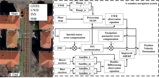
3. High-Precision Indoor Positioning for AVs

For use in an indoor environment similar to an underground parking lot, a TC UWB/INS/map scheme is proposed for the high-precision indoor navigation and positioning of AVs. In this research, the INS and map information are fully utilized to identify the NLOS propagation of UWB signals and eliminate the influence of NLOS errors.

3.1. INS Dynamics Model for the TC UWB/INS/Map Integrated System

In the TC integrated UWB/INS/map system model, as shown in

Table 1. Description of the coordinate system.

Coordinate System	Description
The inertial frame (i-frame)	The i-frame is an ideal frame of reference in which ideal accelerometers and gyroscopes fixed to the i-frame have zero outputs.
The body frame (b-frame)	The b-frame is the frame in which the accelerations and angular rates generated by the strapdown accelerometers and gyroscopes are resolved, i.e., the forward–right–down system.
The navigation frame (n-frame)	The n-frame is selected as the navigation solution coordinate system. The n-frame is a local geodetic frame that has its origin coinciding with that of the sensor frame, i.e., the north–east–down (NED) system.
The Earth frame (e-frame)	The e-frame has its origin at the center of mass of the Earth and axes that are fixed with respect to the Earth.

, several coordinate systems are used.

An error analysis is performed in an n-frame coordinate system for the calculated position at the local level. The $\mathit{\psi }$ angle error model is summarized as follows [32,33]:

$$\left\{\begin{array}{c}\delta {\dot{\mathit{r}}}^n=-{\mathit{\omega }}_{en}^n\delta {\mathit{r}}^n+\delta {\mathit{v}}^n\\ \delta {\dot{\mathit{v}}}^n=\delta {\mathit{g}}^n-(2{\mathit{\omega }}_{ie}^n+{\mathit{\omega }}_{en}^n)\times \delta {\mathit{v}}^n+{\mathit{f}}^n\times {\mathit{\psi }}^n+{\mathit{C}}_b^n[{\mathit{b}}_a+\mathrm{diag}\left({\mathit{f}}^b\right){\mathit{s}}_a]\\ {\dot{\mathit{\psi }}}^n=-({\mathit{\omega }}_{ie}^n+{\mathit{\omega }}_{en}^n)\times {\mathit{\psi }}^n-{\mathit{C}}_b^n[{\mathit{b}}_g+\mathrm{diag}\left({\mathit{\omega }}_{ib}^b\right){\mathit{s}}_g]\end{array}\right.$$

(1)

Here, $\delta {\mathit{r}}^n$, $\delta {\mathit{v}}^n$, and ${\mathit{\psi }}^n$ are error vectors of the IMU position, velocity, and attitude, respectively, in the n-frame. $\delta {\dot{\mathit{r}}}^n$, $\delta {\dot{\mathit{v}}}^n$, and ${\dot{\mathit{\psi }}}^n$ are the time derivatives of the corresponding error vectors in the n-frame. ${\mathit{\omega }}_{en}^n$ denotes the n-frame projection of the angular rate of the n-frame with respect to the e-frame. ${\mathit{\omega }}_{ie}^n$ denotes the n-frame projection of the magnitude of the rotation rate of the Earth. $\delta {\mathit{g}}^n$ denotes the projection of the gravity error vector in the n-frame. ${\mathit{f}}^n={\mathit{C}}_b^n{\mathit{f}}^b$ is the specific force vector in the n-frame. ${\mathit{C}}_b^n$ represents the rotation matrix of the b-frame with respect to the n-frame. It is assumed that the current geographic coordinate is $(\lambda ,\varphi ,h)$, which represents the longitude, latitude, and height of the geographic coordinates of the point. Assuming $(\alpha ,\chi ,\kappa )$ is the Euler angle from the n-frame to the b-frame, ${\mathit{C}}_b^n$, ${\mathit{\omega }}_{ie}^n$, ${\mathit{\omega }}_{en}^n$, and $\delta {\mathit{g}}^n$ can be expressed as follows:

$$\begin{array}{c}\hfill \begin{array}{cc}& {\mathit{C}}_b^n=\left[\begin{array}{ccc}cos\kappa cos\chi & cos\kappa sin\chi sin\alpha -sin\kappa cos\alpha & cos\kappa sin\chi cos\alpha +sin\kappa sin\alpha \\ sin\kappa cos\chi & sin\kappa sin\chi sin\alpha +cos\kappa cos\alpha & sin\kappa sin\chi cos\alpha -cos\kappa sin\alpha \\ -sin\chi & cos\chi sin\alpha & cos\chi cos\alpha \end{array}\right]\hfill \\ & {\mathit{\omega }}_{ie}^n={\left[\begin{array}{ccc}{\omega }_{e}cos\varphi & 0& -{\omega }_{e}sin\varphi \end{array}\right]}^{\mathrm{T}}\hfill \\ & {\mathit{\omega }}_{en}^n={\left[\begin{array}{ccc}{\displaystyle \frac{v_E}{R_N+h}}& {\displaystyle \frac{-v_N}{R_M+h}}& {\displaystyle \frac{-v_{E}tan\varphi }{R_N+h}}\end{array}\right]}^{\mathrm{T}}\hfill \\ & \delta {\mathit{g}}^n={\left[\begin{array}{ccc}0& 0& {\displaystyle \frac{2g_l}{\sqrt{R_M{R}_N}+h}}\delta r_D\end{array}\right]}^{\mathrm{T}}\hfill \end{array}\end{array}$$

(2)

where ${\omega }_e$ denotes the magnitude of the rotation rate of the Earth ($7.2921158\times {10}^{-5}$ rad/s). $R_M$ is the meridian radius of curvature, and $R_N$ is the radius of curvature in the prime vertical direction. $g^l$ denotes the current gravity value. $v_N$ and $v_E$ are velocities in the north and east directions, respectively. ${\mathit{\omega }}_{ib}^b$ and ${\mathit{f}}^b$ are the original observations of the angular velocity and specific force of the gyroscope and accelerometer, $\delta {\mathit{\omega }}_{ib}^b={\mathit{b}}_g+\mathrm{diag}\left({\mathit{\omega }}_{ib}^b\right){\mathit{s}}_g$ and $\delta {\mathit{f}}^b={\mathit{b}}_a+\mathrm{diag}\left({\mathit{f}}^b\right){\mathit{s}}_a$, respectively. ${\mathit{b}}_a$ and ${\mathit{s}}_a$ are 3-dimensional vectors, which represent the 3-axis accelerometer bias and scale factor, respectively. ${\mathit{b}}_g$ and ${\mathit{s}}_g$ are three-dimensional vectors, which represent the three-axis gyroscope bias and scale factor, respectively. The biases and scale factors are represented by first-order Gauss–Markov processes [34]:

$$\begin{array}{c}\hfill \dot{\Gamma }\left(t\right)=-\beta \Gamma \left(t\right)+w\left(t\right)\end{array}$$

(3)

where $\beta$ denotes the inverse correlation time constant and $w\left(t\right)$ denotes white Gaussian noise excitation.

Most of the random system modeling performed in practical applications is continuous in time. The continuous-time linear random system can be expressed as

$$\begin{array}{c}\hfill \dot{\mathit{X}}\left(t\right)=\mathit{F}\left(t\right)\mathit{X}\left(t\right)+\mathit{G}\left(t\right)\mathit{w}\left(t\right)\end{array}$$

(4)

where $\mathit{F}\left(t\right)$ and $\mathit{G}\left(t\right)$ are deterministic time-varying matrices expressed in terms of the time parameter t, and $\mathit{w}\left(t\right)$ is a zero-mean white Gaussian noise vector. According to Equation (1), $\mathit{F}\left(t\right)$ can be expressed as

$$\begin{array}{c}\hfill \begin{array}{c}\hfill \mathit{F}\left(t\right)=\left[\begin{array}{ccccccc}{\mathit{F}}_{11}& \mathit{I}& \mathbf{0}& \mathbf{0}& \mathbf{0}& \mathbf{0}& \mathbf{0}\\ {\mathit{F}}_{21}& {\mathit{F}}_{21}& ({\mathit{f}}^n\times )& \mathbf{0}& {\mathit{C}}_b^n& \mathbf{0}& {\mathit{F}}_{27}\\ \mathbf{0}& \mathbf{0}& {\mathit{F}}_{33}& -{\mathit{C}}_b^n& \mathbf{0}& {\mathit{F}}_{36}& \mathbf{0}\\ \mathbf{0}& \mathbf{0}& \mathbf{0}& {\mathit{F}}_{44}& \mathbf{0}& \mathbf{0}& \mathbf{0}\\ \mathbf{0}& \mathbf{0}& \mathbf{0}& \mathbf{0}& {\mathit{F}}_{55}& \mathbf{0}& \mathbf{0}\\ \mathbf{0}& \mathbf{0}& \mathbf{0}& \mathbf{0}& \mathbf{0}& {\mathit{F}}_{66}& \mathbf{0}\\ \mathbf{0}& \mathbf{0}& \mathbf{0}& \mathbf{0}& \mathbf{0}& \mathbf{0}& {\mathit{F}}_{77}\end{array}\right]\end{array}\end{array}$$

(5)

where ${\mathit{F}}_{11}=-({\omega }_{en}^n\times )$, ${\mathit{F}}_{21}=diag(-{\mathit{\omega }}_s^2-{\mathit{\omega }}_s^{2}2{\mathit{\omega }}_s^2)$, ${\mathit{F}}_{22}=-[(2{\mathit{\omega }}_{ie}^n+{\mathit{\omega }}_{en}^n)\times ]$, ${\mathit{F}}_{27}={\mathit{C}}_b^n\mathrm{diag}\left({\mathit{f}}^b\right)$, ${\mathit{F}}_{33}=-[({\mathit{\omega }}_{ie}^n+{\mathit{\omega }}_{en}^n)\times ]$, ${\mathit{F}}_{36}={\mathit{C}}_b^n\mathrm{diag}\left({\mathit{\omega }}_{ib}^b\right)$, and ${\mathit{\omega }}_s$ denotes the Schuler angular frequency. ${\mathit{F}}_{44}=-\mathrm{diag}\left(T_{gb}^{-1}{T}_{gb}^{-1}{T}_{gb}^{-1}\right)$, ${\mathit{F}}_{55}=-\mathrm{diag}\left(T_{ab}^{-1}{T}_{ab}^{-1}{T}_{ab}^{-1}\right)$, ${\mathit{F}}_{66}=-\mathrm{diag}\left(T_{gs}^{-1}{T}_{gs}^{-1}{T}_{gs}^{-1}\right)$, and ${\mathit{F}}_{77}=-\mathrm{diag}\left(T_{as}^{-1}{T}_{as}^{-1}{T}_{as}^{-1}\right)$. Because the errors of inertial sensors are modeled as first-order Gauss–Markov processes, ${\mathit{F}}_{44}$, ${\mathit{F}}_{55}$, ${\mathit{F}}_{66}$, and ${\mathit{F}}_{77}$ are the corresponding correlation time coefficient matrices. $T_{gb}^{-1},T_{ab}^{-1},T_{gs}^{-1}, \mathrm{and} T_{as}^{-1}$ are Markov process-related times, which depend on the performance of INS and are set to 4 h in this article.

$$\begin{array}{c}\hfill \begin{array}{cc}& \mathit{G}\left(t\right)=diag\left(\mathbf{0}{\mathit{C}}_b^n{\mathit{C}}_b^n\mathit{I}\mathit{I}\mathit{I}\mathit{I}\right)\hfill \\ & \mathit{w}\left(t\right)={\left[\mathbf{0}{\mathit{w}}_v{\mathit{w}}_{\psi }{\mathit{w}}_{gb}{\mathit{w}}_{ab}{\mathit{w}}_{gs}{\mathit{w}}_{as}\right]}^{\mathrm{T}}\hfill \end{array}\end{array}$$

(6)

where ${\mathit{w}}_v$ is the white noise of the accelerometer measurement error. ${\mathit{w}}_{\psi }$ is the white noise of the gyroscope measurement error. ${\mathit{w}}_{gb}$ and ${\mathit{w}}_{ab}$ are the driven noise of the gyroscope and accelerometer biases, respectively. ${\mathit{w}}_{gs}$ and ${\mathit{w}}_{as}$ are the driven noise of the gyroscope and accelerometer scale factors, respectively.

According to linear theory, to perform filter estimation, the continuous-time system of Equation (4) needs to be discretized:

$$\begin{array}{c}\hfill \begin{array}{cc}& {\mathit{X}}_k={\mathit{\Phi }}_{k/k-1}{\mathit{X}}_{k-1}+{\mathit{\eta }}_{k-1}\hfill \\ & {\mathit{X}}_k=\mathit{X}\left(t_k\right)\hfill \\ & {\mathit{\Phi }}_{k/k-1}\approx \mathit{I}+\mathit{F}\left(t_{k-1}\right)T_s\hfill \end{array}\end{array}$$

(7)

Here, ${\mathit{X}}_k$ and ${\mathit{X}}_{k-1}$ denote the state vectors after discretization. ${\mathit{\Phi }}_{k/k-1}$ denotes the state transition matrix. ${\mathit{\eta }}_{k-1}$ denotes the linear transformation of the white Gaussian noise $\mathit{w}\left(\tau \right)$. $\mathit{I}$ denotes identity matrix. $T_s=0.005$ s represents the time interval, which is determined by the IMU frequency 200 Hz.

By combining Equations (1) and (3), the state of the integrated system can be generated in discrete vector form by using Equation (7), resulting in a 21-dimensional vector of the following form:

$$\begin{array}{c}\hfill \begin{array}{c}\hfill {\mathit{X}}_k={\left[\delta {\mathit{r}}^n\delta {\mathit{v}}^n{\mathit{\psi }}^n{\mathit{b}}_g{\mathit{b}}_a{\mathit{s}}_g{\mathit{s}}_a\right]}^{\mathrm{T}}\end{array}\end{array}$$

(8)

3.2. NLOS Error Recognition and Elimination Based on UWB/INS/Map Integration

Indoor structures generally have regular shapes. These structures include walls, metal doors, glass, and some fixed facilities whose location information is an important part of indoor maps. Therefore, high-precision maps for specific indoor scenes can be easily obtained. These structures serve as obstacles that affect UWB ranging signals, resulting in decreased ranging accuracy. Consequently, it is possible to make full use of indoor map information to control the quality of UWB data to prevent degradation in the accuracy of a seamless navigation system. The proposed TC UWB/INS/map integration method attempts to eliminate the impact of NLOS errors. The prior information from a map and an INS is used in this paper to identify UWB NLOS errors. As shown in Figure 1, when an AV travels to an arbitrary position, this prior information can be used to quickly determine the occlusion of UWB observations. Specifically, each red dashed line in Figure 1 is drawn between the high-precision position of the mobile UWB node provided by the INS mechanism and the position of a UWB anchor node. Then, the key to judging the occlusion of UWB observations lies in judging whether each red dashed line intersects with any line segment information in the map. The number n of intersection points between each red dashed line and line segments in the map is counted to determine the status of signal blockage by obstacles between the mobile UWB node and the corresponding anchor node at the current moment. The larger the value of n is, the more severely the UWB signal propagation is affected by surrounding obstacles. Based on experience from many experiments, the UWB NLOS ranging value can be modeled, and the following formula for UWB NLOS error reduction can be established [35]:

$$\begin{array}{c}\hfill V_i=\left\{\begin{array}{cc}{v}_i\hfill & n=0\hfill \\ n\beta \ast v_i\hfill & 0<n<3\hfill \\ +\infty \hfill & 3\le n\hfill \end{array}\right.\end{array}$$

(9)

where $V_i$ is the real measurement noise adjusted based on the map, $v_i$ denotes the UWB measurement noise in a line-of-sight (LOS) environment, and $\beta$ is a constant that represents an expansion factor introduced into the measurement noise, usually chosen to have a value of 10–20. Both in theory and in practice, the constant $\beta$ can be determined on the basis of the unique properties of the UWB signal and the objective conditions of the environment.

Based on Equation (9), the measurement noise of the UWB observations can be adjusted by reducing the weight of an observation or discarding an observation.

3.3. Measurement Model for the TC UWB/INS/Map Integrated System

In the TC UWB/INS/map model, the UWB positioning coordinate system chosen can be either the e-frame or the n-frame. If it is difficult to unify the systems for indoor and outdoor spaces, a custom coordinate system can also be selected. In this paper, the e-frame is adopted as the unified coordinate system to unify the indoor and outdoor coordinate systems. The mobile UWB node position ${\mathit{r}}_{INS}^e$ calculated by the INS can be deduced from the IMU position ${\mathit{r}}_{IMU}^e$, and the disturbance analysis is as follows:

$$\begin{array}{c}\hfill \begin{array}{cc}\hfill {\tilde{\mathit{r}}}_{INS}^e={\mathit{C}}_n^e{\tilde{\mathit{r}}}_{INS}^n& ={\mathit{C}}_n^e{\tilde{\mathit{r}}}_{IMU}^n+{\mathit{C}}_n^e{\tilde{\mathit{C}}}_b^n{\mathit{l}}_{UWB}^b\hfill \\ & ={\mathit{C}}_n^e({\mathit{r}}_{IMU}^n+\delta {\mathit{r}}^n)+{\mathit{C}}_n^e(\mathit{I}-{\mathit{\psi }}^n\times ){\mathit{C}}_b^n{\mathit{l}}_{UWB}^b\hfill \\ & ={\mathit{C}}_n^e{\mathit{r}}_{IMU}^n+{\mathit{C}}_n^e{\mathit{C}}_b^n{\mathit{l}}_{UWB}^b+{\mathit{C}}_n^e\delta {\mathit{r}}^n+{\mathit{C}}_n^e(-{\mathit{\psi }}^n\times ){\mathit{C}}_b^n{\mathit{l}}_{UWB}^b\hfill \\ & ={\mathit{C}}_n^e{\mathit{r}}_{UWB}^n+{\mathit{C}}_n^e\delta {\mathit{r}}^n+{\mathit{C}}_n^e({\mathit{C}}_b^n{\mathit{l}}_{UWB}^b\times ){\mathit{\psi }}^n\hfill \end{array}\end{array}$$

(10)

where $\widetilde{•}$ denotes a disturbed term, and ${\mathit{r}}_{INS}^e$ and ${\mathit{r}}_{INS}^n$ represent the position coordinates in the e-frame and n-frame for the mobile UWB node as calculated by the INS, respectively. ${\mathit{r}}_{IMU}^n$ represents the position coordinates of the center of the IMU in the n-frame, and $\delta {\mathit{r}}^n$ is the same as the IMU position error in the state vector of Equation (8). ${\mathit{l}}_{UWB}^b$ is the accurately measured lever-arm vector in the b-frame, which is considered to be error-free, and ${\mathit{C}}_n^e$ denotes the rotation matrix of the n-frame with respect to the e-frame, and because the $\psi$ model is used, the n-frame can be considered known and there is no need to perform disturbance analysis on ${\mathit{C}}_n^e$.

$$\begin{array}{c}\hfill {\mathit{C}}_n^e=\left[\begin{array}{ccc}-sin\varphi cos\lambda & -sin\lambda & -cos\varphi cos\lambda \\ -sin\varphi sin\lambda & cos\lambda & -cos\varphi sin\lambda \\ cos\varphi & 0& sin\varphi \end{array}\right]\end{array}$$

(11)

${\mathit{r}}_{UWB}^n$ denotes the actual location of the mobile UWB node in the n-frame. The UWB observation equation can be written as follows:

$$\begin{array}{c}\hfill \begin{array}{c}\hfill {\tilde{\mathit{d}}}_{UWB}={\parallel {\tilde{\mathit{r}}}_{UWB}^e-{\mathit{r}}_{anchor}^e\parallel }_2\end{array}\end{array}$$

(12)

where ${\tilde{\mathit{d}}}_{UWB}$ denotes the UWB observation, ${\tilde{\mathit{r}}}_{UWB}^e$ is the mobile UWB node position with disturbance in the e-frame, ${\mathit{r}}_{anchor}^e$ denotes the position of a UWB anchor node with known coordinates, which is measured in advance by Leica TS50 automatic tracking total station, and it is assumed that there is no error; ${\parallel •\parallel }_2$ is the Euclidean distance. For brevity, the error $\delta {\mathit{r}}_{INS}^e$ between the position ${\tilde{\mathit{r}}}_{UWB}^e$ of the mobile UWB node and the position ${\tilde{\mathit{r}}}_{INS}^e$ calculated by the INS can be written as

$$\begin{array}{c}\hfill \begin{array}{cc}\hfill \delta {\mathit{r}}_{INS}^e& ={\tilde{\mathit{r}}}_{UWB}^e-{\tilde{\mathit{r}}}_{INS}^e\hfill \\ & \approx {\mathit{C}}_n^e\delta {\mathit{r}}^n+{\mathit{C}}_n^e({\mathit{C}}_b^n{\mathit{l}}_{UWB}^b\times ){\mathit{\psi }}^n\hfill \end{array}\end{array}$$

(13)

In the construction of the TC UWB/INS/map observation model, the UWB observation function is expanded using the Taylor formula at the approximate position ${\mathit{x}}_0={\tilde{\mathit{r}}}_{INS}^e$ to obtain the TC UWB/INS/map observation equation as follows:

$$\begin{array}{c}\hfill \begin{array}{c}\hfill {\tilde{\mathit{d}}}_{UWB}-{\mathit{d}}_{INS}=\frac{{({\tilde{\mathit{r}}}_{INS}^e-{\mathit{r}}_{anchor}^e)}^T}{{\mathit{d}}_{INS}}{\mathit{C}}_n^e\delta {\mathit{r}}^n+\frac{{({\tilde{\mathit{r}}}_{INS}^e-{\mathit{r}}_{anchor}^e)}^T}{{\mathit{d}}_{INS}}{\mathit{C}}_n^e({\mathit{C}}_b^n{\mathit{l}}_{UWB}^b\times ){\mathit{\psi }}^n+{\mathit{\epsilon }}_u\end{array}\end{array}$$

(14)

where ${\tilde{d}}_{INS}$ and $d_{INS}$ denote the UWB observation and the INS-predicted range, respectively; ${\mathit{\epsilon }}_u$ represents the noise sequence.

Consequently, the discrete UWB/INS/map measurement model can be expressed as follows:

$$\begin{array}{c}\hfill \begin{array}{c}\hfill {\mathit{Z}}_k={\mathit{H}}_k{\mathit{X}}_k+{\mathit{V}}_k\end{array}\end{array}$$

(15)

where ${\mathit{Z}}_k$ is an m-dimensional measurement vector, ${\mathit{H}}_k$ is a measurement matrix with dimensions of $m\times 21$, and ${\mathit{V}}_k$ is an m-dimensional measurement noise vector. m depends on the number of effective UWB observations. After the UWB/INS/map system is used to identify and weaken or discard UWB observations affected by NLOS errors, ${\mathit{V}}_k$ is approximately a white Gaussian noise sequence with zero mean. Equation (15) can then be rewritten as follows:

$$\begin{array}{c}\hfill \begin{array}{cc}& {\mathit{Z}}_k=[{\tilde{d}}_{UWB}-d_{INS}]\hfill \\ & {\mathit{H}}_k=\left[{\mathit{H}}_{UWB}^e{\mathit{C}}_n^e{\mathbf{0}}_{m\times 3}{\mathit{H}}_{UWB}^e{\mathit{C}}_n^e({\mathit{C}}_b^n{\mathit{l}}_{UWB}^b\times ){\mathbf{0}}_{m\times 12}\right]\hfill \end{array}\end{array}$$

(16)

where ${\mathit{H}}_{UWB}^e$ is the linearized matrix in the UWB/INS/map observation equation.

In a challenging indoor environment, the NLOS propagation of UWB signals affects the ranging accuracy. Moreover, multipath propagation, propagation interference, etc., affect the ranging accuracy. Hence, the use of map and INS information to identify the NLOS propagation of signals cannot, by itself, meet the high-precision requirements for AVs. To mitigate the effects of multipath propagation, propagation interference, system noise, and unidentified NLOS errors, an improved AREKF algorithm is proposed for use in complex indoor environments. This algorithm is introduced in Section 4.2.

4. High-Precision and Seamless Positioning for AVs in Harsh Environments

The positioning of an AV in the transitional environment between indoor and outdoor environments is another challenging problem. In this transitional environment, the number of GNSS satellites is small, their geometric distribution is poor, and their signals are severely affected by multipath effects. Therefore, an improved AREKF algorithm based on a single-frequency integrated multi-GNSS-TC RTK/INS/UWB/map system is proposed to solve the positioning problem for AVs in transitional environments. In this TC integrated system, the GNSS code and carrier phase observations are susceptible to multipath errors. The code observations are particularly affected by multipath effects, and the UWB ranging accuracy is affected by multipath propagation. Observations with large errors seriously affect the accuracy of floating-point solutions in the GNSS calculation process, thereby affecting the success rate of ambiguity resolution. To reduce the influence of measurement outliers on parameter estimation, the improved AREKF algorithm is introduced to adjust the variance of outliers. The algorithm flowchart is shown in Figure 2.

4.1. Measurement Model of the TC Integrated Multi-GNSS-TC RTK/INS/UWB/Map System

On the basis of the respective internal double-difference (DD) observation equations of GNSSs, multi-GNSS-TC RTK implies that in each system (including GPS, the BeiDou Navigation Satellite System (BDS), Galileo, and the Global Navigation Satellite System (GLONASS)), only one suitable satellite is selected as a reference, the deviations between the different satellite systems are estimated, and the different satellite systems are tightly combined to construct DD observation equations between the systems. In the process of multi-GNSS-TC RTK, the space data and time reference data between different GNSSs need to be unified using known parameters and methods [36]. The multi-GNSS-TC RTK method establishes DD observation equations between different satellite systems and increases the number of redundant observations in a challenging transitional environment. The success rate of ambiguity resolution between different satellite systems is improved. However, the effects of receiver hardware delay differences, and signal frequency differences on the ambiguity must be considered in the multi-GNSS-TC RTK method due to the existence of systems with different signal modulation methods. The unified DD observation model of multi-GNSS-TC RTK includes an internal DD observation model of a GNSS that uses code-division multiple access (CDMA) technology, an internal DD observation model of a GNSS that uses frequency-division multiple access (FDMA) technology, a DD observation model between GNSSs that use CDMA technology, and a DD observation model between a GNSS that uses CDMA technology and a GNSS that uses FDMA technology [37]. Considering the hardware delay and the initial phase deviation, the pseudorange and phase undifferenced observation equations can be expressed as follows:

$$\begin{array}{c}\hfill \begin{array}{cc}\hfill L_{a,j}^{M_s}=& {\rho }_a^{M_s}+d{t}_a+d{t}^{M_s}+T_a^{M_s}-I_{a,j}^{M_s}+{\lambda }_j^{M_s}({\delta }_{a,j}^{M_s}+{\phi }_{a,j}^{M_s}-{\delta }_{,j}^{M_s}-{\phi }_{,j}^{M_s}+N_{a,j}^{M_s})\hfill \\ & +d_{GMTO}+{\epsilon }_{a,j}^{M_s}\hfill \\ \hfill P_{a,j}^{M_s}=& {\rho }_a^{M_s}+d{t}_a+d{t}^{M_s}+T_a^{M_s}+I_{a,j}^{M_s}+{\beta }_{a,j}^{M_s}-{\beta }_{,j}^{M_s}+d_{GMTO}+{\xi }_{a,j}^{M_s}\hfill \end{array}\end{array}$$

(17)

Here, M denotes the GNSS in which the observation is made, which can be GPS, GLONASS, BDS, or Galileo. s is an index denoting a specific satellite in system M. Similarly, a is an index denoting a specific receiver, and j is an index denoting a specific frequency band for tracking satellites. L and P represent phase and pseudorange observations, respectively. ${\rho }_a^{M_s}$ is the geometric distance from receiver a to satellite $M_s$. $d{t}_a$ is the clock error of receiver a. $d{t}^{M_s}$ is the clock error of satellite $M_s$. $T_a^{M_s}$ is the tropospheric delay. $I_{a,j}^{M_s}$ is the ionospheric delay. ${\lambda }_j^{M_s}$ is the wavelength of GNSS satellite $M_s$ in the j-th frequency band. ${\delta }_{a,j}^{M_s}$ and ${\beta }_{a,j}^{M_s}$ are the hardware delays of the GNSS receiver phase and pseudorange, respectively, in the j-th frequency band. ${\delta }_{,j}^{M_s}$ and ${\beta }_{,j}^{M_s}$ are the hardware delays of the GNSS satellite phase and pseudorange, respectively, in the j-th frequency band. ${\phi }_{a,j}^{M_s}$ and ${\phi }_{,j}^{M_s}$ are the initial phase deviations of the GNSS receiver and satellite, respectively. $N_{a,j}^{M_s}$ is the undifferenced ambiguity with integer characteristics. $d_{GMTO}$ is the time system deviation of system M, where the GPS system and GPS time (GPST) are used as the reference. ${\epsilon }_{a,j}^{M_s}$ and ${\xi }_{a,j}^{M_s}$ are the observation noise of the phase and pseudorange, respectively.

After the observation equations of two GNSS receivers a and b undergo single differencing, the satellite clock error, hardware delay, initial phase deviation, orbit error, and time system deviation are all eliminated. Under short-baseline conditions, both the tropospheric and ionospheric delays in the single-difference (SD) case can be ignored. The SD phase and pseudorange observation equations between GNSS stations can be expressed as follows:

$$\begin{array}{c}\hfill \begin{array}{cc}& L_{ab,j}^{M_s}={\rho }_{ab}^{M_s}+d{t}_{ab}+{\lambda }_j^{M_s}{N}_{ab,j}^{M_s}+{\lambda }_j^{M_s}({\delta }_{ab,j}^{M_s}+{\phi }_{ab,j}^{M_s})+{\epsilon }_{ab,j}^{M_s}\hfill \\ & P_{ab,j}^{M_s}={\rho }_{ab}^{M_s}+d{t}_{ab}+{\beta }_{ab,j}^{M_s}+{\xi }_{ab,j}^{M_s}\hfill \end{array}\end{array}$$

(18)

where ${•}_{ab}$ denotes the SD between receiver a and receiver b and ${\lambda }_j^{M_s}({\delta }_{ab,j}^{M_s}+{\phi }_{ab,j}^{M_s})$ denotes the SD between the base stations of the uncalibrated phase delays (UPDs) at receiver [38]. The processing of ${\lambda }_j^{M_s}({\delta }_{ab,j}^{M_s}+{\phi }_{ab,j}^{M_s})$ depends on whether the current system M uses CDMA technology or FDMA technology, and can be expressed as follows:

$$\begin{array}{c}\hfill {\lambda }_j^{M_s}({\delta }_{ab,j}^{M_s}+{\phi }_{ab,j}^{M_s})=\left\{\begin{array}{cc}{\alpha }_j^M\hfill & CDMA\hfill \\ {\alpha }_j^M+k^{M_s}\mathrm{\Delta }\gamma \hfill & FDMA\hfill \end{array}\right.\end{array}$$

(19)

where ${\alpha }_j^M$ and $\mathrm{\Delta }\gamma$ are the constant term and the rate of change in frequency, respectively, and $k^{M_s}$ denotes the frequency number of a satellite that uses FDMA technology. Substituting Equation (19) into Equation (18) yields the following formulas:

$$\begin{array}{c}\hfill \begin{array}{cc}& L_{ab,j}^{M_s}={\rho }_{ab}^{M_s}+d{t}_{ab}+{\lambda }_j^{M_s}{N}_{ab,j}^{M_s}+{\alpha }_j^M+k^{M_s}\mathrm{\Delta }\gamma +{\epsilon }_{ab,j}^{M_s}\hfill \\ & P_{ab,j}^{M_s}={\rho }_{ab}^{M_s}+d{t}_{ab}+{\beta }_{ab,j}^{M_s}+{\xi }_{ab,j}^{M_s}\hfill \end{array}\end{array}$$

(20)

The signal frequency of the same frequency band may be different for different GNSSs. The effect of different wavelengths on the fixed DD ambiguity is the same, either within a GNSS that uses FDMA technology or between different GNSSs. This paper uses DD ambiguity parameters to be estimated in the form of SD ambiguity parameters. When calculating the difference between satellites $F_l$ and $M_s$, the following DD observation equation is obtained:

$$\begin{array}{c}\hfill \begin{array}{cc}& L_{ab,j}^{F_l{M}_s}={\rho }_{ab}^{F_l{M}_s}+{\lambda }_j^{M_s}{N}_{ab,j}^{M_s}-{\lambda }_j^{F_l}{N}_{ab,j}^{F_l}+{\alpha }_j^{FM}+(k^{M_s}-k^{F_l})\mathrm{\Delta }\gamma +{\epsilon }_{ab,j}^{F_l{M}_s}\hfill \\ & P_{ab,j}^{F_l{M}_s}={\rho }_{ab}^{F_l{M}_s}+{\beta }_{ab,j}^{F_l{M}_s}+{\xi }_{ab,j}^{F_l{M}_s}\hfill \end{array}\end{array}$$

(21)

where ${•}^{F_l{M}_s}$ denotes the DD between satellite $F_l$ and satellite $M_l$. The receiver clock error $d{t}_{ab}$ is eliminated. $F_l$ denotes the l-th satellite of satellite system F. The values and meanings of ${\alpha }_j^{FM}$, $k^{M_s}$, $k^{F_l}$, and $\mathrm{\Delta }\gamma$ differ depending on whether F and M are the same and whether the multiple access technologies used are the same [37]:

• Both satellite systems use CDMA signal modulation: ${\alpha }_j^{FM}$, $k^{M_s}$, $k^{F_l}$, and $\mathrm{\Delta }\gamma$ are all equal to zero.
• Both satellite systems use FDMA signal modulation: ${\alpha }_j^{FM}=0$, $k^{M_s}$, and $k^{F_l}$ are the frequency numbers of the two different GLONASS satellites, and $\mathrm{\Delta }\gamma$ is the rate of change of the interfrequency bias (IFB).
• The two satellite systems are different, but both adopt CDMA signal modulation: ${\alpha }_j^{FM}$ is the intersystem bias (ISB) in the system phase, and $k^{M_s}$, $k^{F_l}$, and $\mathrm{\Delta }\gamma$ are all equal to zero.
• The two satellite systems are different and adopt different types of signal modulation: ${\alpha }_j^{FM}$ denotes the intersatellite phase ISB of the two satellites for frequency number 0, $k^{F_l}=0$, $k^{M_s}$ is the frequency number of the GLONASS satellite, and $\mathrm{\Delta }\gamma$ is the rate of change of the IFB.

Equation (21) is a nonlinear equation. Taylor series expansion is performed around the GNSS receiver antenna phase $r_{INS}^e$ calculated by the INS, following a process similar to that of Equations (10), (13), and (14), to obtain a unified multi-GNSS-TC RTK/INS observation model:

$$\begin{array}{c}\hfill \begin{array}{cc}\hfill L_{ab,j}^{F_l{M}_s}-{\rho }_{ab,INS}^{F_l{M}_s}=& {\mathit{H}}_G^e{\mathit{C}}_n^e\delta {\mathit{r}}^n+({\mathit{H}}_G^e{\mathit{C}}_n^e{\mathit{C}}_b^n{\mathit{l}}_{GNSS}^b\times ){\mathit{\psi }}^n+{\lambda }_j^{M_s}{N}_{ab,j}^{M_s}-{\lambda }_{ab,j}^{F_l}{N}_{ab,j}^{F_l}\hfill \\ & +{\alpha }_j^{FM}+(k^{M_s}-k^{F_l})\mathrm{\Delta }\gamma +{\epsilon }_{ab,j}^{F_l{M}_s}\hfill \\ \hfill P_{ab,j}^{F_l{M}_s}-{\rho }_{ab,INS}^{F_l{M}_s}=& {\mathit{H}}_G^e{\mathit{C}}_n^e\delta {\mathit{r}}^n+({\mathit{H}}_G^e{\mathit{C}}_n^e{\mathit{C}}_b^n{\mathit{l}}_{GNSS}^b\times ){\mathit{\psi }}^n+{\beta }_{ab,j}^{F_l{M}_s}+{\xi }_{ab,j}^{F_l{M}_s}\hfill \end{array}\end{array}$$

(22)

where ${\rho }_{ab,INS}^{F_l{M}_s}$ is the DD geometric distance calculated between the receiver coordinates provided by the INS and the satellite coordinates and ${\mathit{H}}_G^e$ is the linearized matrix in the multi-GNSS RTK/INS observation equation.

By combining and rearranging Equations (14) and (22), the TC integrated multi-GNSS-TC RTK/INS/UWB/map observation equation, which considers the system bias, is obtained as follows:

$$\begin{array}{c}\hfill \begin{array}{cc}\hfill L_{ab,j}^{F_l{M}_s}-{\rho }_{ab,INS}^{F_l{M}_s}=& {\mathit{H}}_G^e{\mathit{C}}_n^e\delta {\mathit{r}}^n+({\mathit{H}}_G^e{\mathit{C}}_n^e{\mathit{C}}_b^n{\mathit{l}}_{GNSS}^b\times ){\mathit{\psi }}^n+{\lambda }_j^{M_s}{N}_{ab,j}^{M_s}-{\lambda }_{ab,j}^{F_l}{N}_{ab,j}^{F_l}\hfill \\ & +{\alpha }_j^{FM}+(k^{M_s}-k^{F_l})\mathrm{\Delta }\gamma +{\epsilon }_{ab,j}^{F_l{M}_s}\hfill \\ \hfill P_{ab,j}^{F_l{M}_s}-{\rho }_{ab,INS}^{F_l{M}_s}=& {\mathit{H}}_G^e{\mathit{C}}_n^e\delta {\mathit{r}}^n+({\mathit{H}}_G^e{\mathit{C}}_n^e{\mathit{C}}_b^n{\mathit{l}}_{GNSS}^b\times ){\mathit{\psi }}^n+{\beta }_{ab,j}^{F_l{M}_s}+{\xi }_{ab,j}^{F_l{M}_s}\hfill \\ \hfill {\tilde{d}}_{UWB}-d_{INS}=& {\mathit{H}}_{UWB}^e{\mathit{C}}_n^e\delta {\mathit{r}}^n+{\mathit{H}}_{UWB}^e{\mathit{C}}_n^e({\mathit{C}}_b^n{\mathit{l}}_{UWB}^b\times ){\mathit{\psi }}^n+{\mathit{\epsilon }}_u\hfill \end{array}\end{array}$$

(23)

Therefore, the error vector of the TC integrated multi-GNSS-TC RTK/INS/UWB/map is as follows:

$$\begin{array}{c}\hfill \begin{array}{c}\hfill {\mathit{X}}_k={\left[\delta {\mathit{r}}^n\delta {\mathit{v}}^n{\mathit{\psi }}^n{\mathit{b}}_g{\mathit{b}}_a{\mathit{s}}_g{\mathit{s}}_a\delta \mathit{N}\right]}^{\mathrm{T}}\end{array}\end{array}$$

(24)

where $\delta \mathit{N}$ are the ambiguity error vectors of the GNSS system. Notably, when the carrier phase ambiguities are not fixed, the TC integrated system uses the pseudorange and carrier phase observation values to filter and update, respectively, and attempts to fix the ambiguity of the obtained floating-point solution of the ambiguity. When the ambiguity is resolved, the ambiguity parameters in the system state vector need to be eliminated, and the state vector is Equation (8).

4.2. An Improved Innovation-Based AREKF Algorithm to Resist Outliers

As mentioned above, an improved AREKF algorithm is proposed for application in a complex indoor environment to resist abnormal UWB observations, which are affected by multipath propagation, environmental interference, system noise, etc. Similarly, GNSS pseudorange and carrier phase observations are easily affected by multipath effects in a complex urban environment. In the transitional environment between outdoors and indoors, GNSS and UWB observations are particularly susceptible to noise, the error of the GNSS pseudorange observations will exceed the meter level, and the ambiguity parameter of the GNSS carrier phase observations is not easy to fix. If the UWB observations are affected by the NLOS environment, the UWB error will also exceed the meter level. Observations with these large errors will affect the performance of an integrated navigation system, significantly reducing the accuracy of the floating-point resolution and ultimately reducing the accuracy of the solution results. Therefore, before the tight combination of the multi-GNSS-TC RTK/INS/UWB/map systems, the UWB NLOS error is first identified and suppressed, and then outlier detection is performed on the GNSS and UWB observation information. An INS offers high accuracy over a short time and has advantages in detecting outliers in GNSS and UWB observations. In this paper, the innovation of the EKF is used to adaptively adjust the noise matrix of the observations, making the filtering system robust. The standardized innovation ${\tilde{v}}_{k,i}$ of the EKF can be expressed as follows:

$$\begin{array}{c}\hfill {\tilde{v}}_{k,i}=\frac{{({\mathit{Z}}_k-{\mathit{H}}_k{\widehat{\mathit{X}}}_k^{-})}_i}{\sqrt{{({\mathit{H}}_k{\mathit{P}}_k^{-}{\mathit{H}}_k^T+\mathit{R})}_{i,i}}}\end{array}$$

(25)

where ${\mathit{Z}}_k$ is the observation vector, ${\mathit{H}}_k$ is the observation coefficient matrix, ${\widehat{\mathit{X}}}_k^{-}$ is the state prediction, ${\mathit{P}}_k^{-}$ is the predicted state error covariance matrix, and $\mathit{R}$ is the observation noise covariance matrix. An adjustment factor is constructed based on the robust estimation for correlated observations (RECO) scheme [39]:

$$\begin{array}{c}\hfill {\gamma }_{ii}=\left\{\begin{array}{cc}1\hfill & |v_{k,i}|\le k_0\hfill \\ \frac{|v_{k,i}|}{k_0}\times (\frac{k_1-k_0}{k_1-\left|v_{k,i}\right|})\hfill & k_0<\left|v_{k,i}\right|\le k_1\hfill \\ +\infty \hfill & |v_{k,i}|>k_1\hfill \end{array}\right.\end{array}$$

(26)

where $k_0$ and $k_1$ are two empirical constants, which are usually considered to be in the ranges of 2.0–3.0 and 4.5–8.5, respectively [39]. When the accuracy of the observations is stable, the adjustment factor is equal to 1; when the observation values are severely abnormal, the adjustment factor is infinite, and observation anomalies do not affect the state estimation; and when the innovation sequence is between $k_0$ and $k_1$, the influence of observation anomalies is weakened. Thus, the adaptively adjusted observation noise covariance matrix $\overline{\mathit{R}}$ before the EKF measurement update is obtained as follows:

$$\begin{array}{c}\hfill \begin{array}{cc}& \overline{\mathit{R}}=\left[\begin{array}{ccc}{\gamma }_{11}{\sigma }_{11}^2& \cdots & {\gamma }_{1n}{\sigma }_{1n}^2\\ ⋮& \ddots & ⋮\\ {\gamma }_{n1}{\sigma }_{n1}^2& \cdots & {\gamma }_{nn}{\sigma }_{nn}^2\end{array}\right]\hfill \\ & {\gamma }_{ij}=\sqrt{{\gamma }_{ii}{\gamma }_{jj}}\hfill \end{array}\end{array}$$

(27)

where ${\gamma }_{ij}$ is the adjustment factor for the covariance in the i-th row and j-th column [39].

This model assumes that there is no abnormality in the control of the filter system, i.e., observation anomalies are detected and weakened or isolated under the condition that the mean squared error ${\mathit{P}}_k$ and the state estimate ${\widehat{\mathit{X}}}_k$ are not abnormal. However, the mean squared errors of some states will gradually decrease after a long time as the filtering update process continues. Theoretically, the mean squared error will become very small, indicating that the filtering accuracy of the corresponding state is very high. However, random observation noise, often with unknown distributions, will generate erroneous feedback to the system for state estimation due to modeling errors or interference from the complex and changeable observation environment, which will cause state estimation deviations and system model deviations. Consequently, the state estimate will eventually be unable to reach the corresponding estimation accuracy, giving rise to a contradiction between the theoretical accuracy and the actual accuracy, which will cause the system model to fail to either produce the correct state or correctly predict its error level.

In this article, virtual noise injection technology is used to overcome the phenomenon of excessive convergence of the mean squared error of the filter such that the noise has a continuous stimulating effect. To this end, a certain lower bound on the mean squared error is set in accordance with the actual physical meaning of the state or with prior experience. To facilitate the calculation and ensure the positive definiteness of ${\mathit{P}}_k$, the diagonal elements of ${\mathit{P}}_k$ are processed as follows [40]:

$$\begin{array}{c}\hfill {\left({\mathit{P}}_k\right)}_{i,i}<{\left({\mathit{P}}_{min}\right)}_{i,i}\to {\left({\mathit{P}}_k\right)}_{i,i}={\left({\mathit{P}}_{min}\right)}_{i,i}\end{array}$$

(28)

where ${\mathit{P}}_{min}$ is the lower-bound matrix of the mean squared error. When a diagonal element ${\left({\mathit{P}}_k\right)}_{i,i}$ of the updated mean squared error matrix (as measured by the filter) is less than the corresponding lower limit ${\left({\mathit{P}}_{min}\right)}_{i,i}$, it is directly artificially forced to be equal to the lower limit. Similarly, an upper limit to the mean squared error is set to prevent possible filtering anomalies. To ensure the positive definiteness of ${\mathit{P}}_k$, the nondiagonal elements need to be set as follows at the same time [40]:

$$\begin{array}{c}\hfill {\left({\mathit{P}}_k\right)}_{i,i}>{\left({\mathit{P}}_{max}\right)}_{i,i}\to \left\{\begin{array}{c}s=\sqrt{{\left({\mathit{P}}_{max}\right)}_{i,i}/{\left({\mathit{P}}_k\right)}_{i,i}}\hfill \\ {\left({\mathit{P}}_k\right)}_{i,j}={\left.{\left({\mathit{P}}_k\right)}_{i,j}\times s\right|}_{j=1,2,\cdots ,n}\hfill \\ {\left({\mathit{P}}_k\right)}_{j,i}={\left.{\left({\mathit{P}}_k\right)}_{j,i}\times s\right|}_{j=1,2,\cdots ,n}\hfill \end{array}\right.\end{array}$$

(29)

where ${\mathit{P}}_{max}$ is the upper-bound matrix of the mean squared error. When a diagonal mean squared error matrix element ${\left({\mathit{P}}_k\right)}_{i,i}$ exceeds the upper limit ${\left({\mathit{P}}_{max}\right)}_{i,i}$, the i-th row and i-th column elements corresponding to ${\left({\mathit{P}}_k\right)}_{i,i}$ are both reduced by a factor of s simultaneously. Obviously, ${\left({\mathit{P}}_k\right)}_{i,i}$ is guaranteed to have the property of symmetric positive definiteness.

The values of ${\mathit{P}}_{min}$ and ${\mathit{P}}_{max}$ are determined based on experience and sensor performance. The values of ${\mathit{P}}_{max}$ and ${\mathit{P}}_{min}$ in the test cases are set as shown in

Table 2. The values of ${\mathit{P}}_{max}$ and ${\mathit{P}}_{min}$ used in the experiment.

	${\mathit{P}}_{\mathit{max}}$	${\mathit{P}}_{\mathit{min}}$
${\mathit{b}}_g$	1.5°/h	0.01°/h
${\mathit{b}}_a$	30 mGal	5 mGal
${\mathit{s}}_g$	250 ppm	10 ppm
${\mathit{s}}_a$	250 ppm	10 ppm

.

${\mathit{b}}_g$, ${\mathit{b}}_a$, ${\mathit{s}}_g$, and ${\mathit{s}}_a$ are prone to transitional convergence or state abnormality during the experimental calculation. The values of ${\mathit{P}}_{min}$ and ${\mathit{P}}_{max}$ should not be set too large or too small, as this would result in a decrease in the accuracy of filter estimation and cause state fluctuations. Therefore, the biases and scale factors of the accelerometer and gyroscope are mainly constrained in the test cases presented in this article. For the position, velocity, and attitude parameters, ${\mathit{P}}_{min}$ and ${\mathit{P}}_{max}$ are not used for virtual noise injection.

5. Field Experiment Design and Analysis of Results

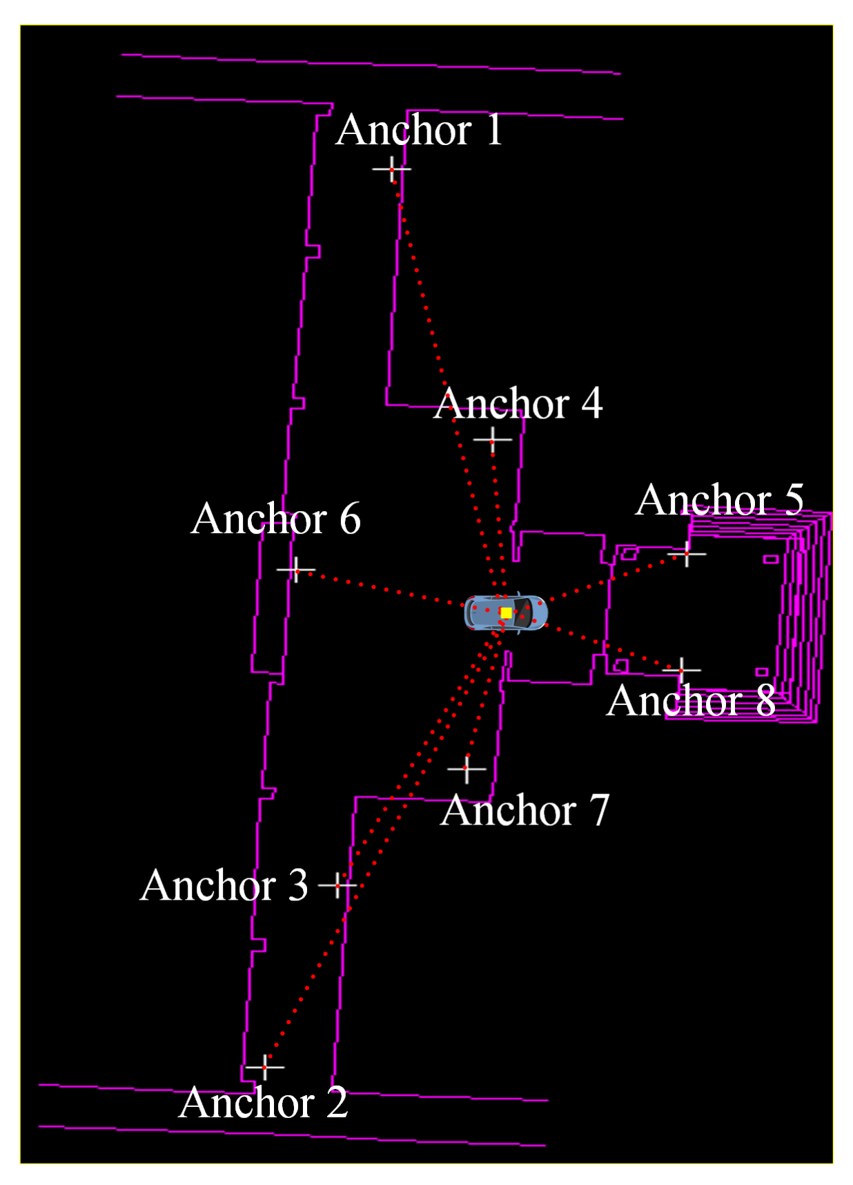
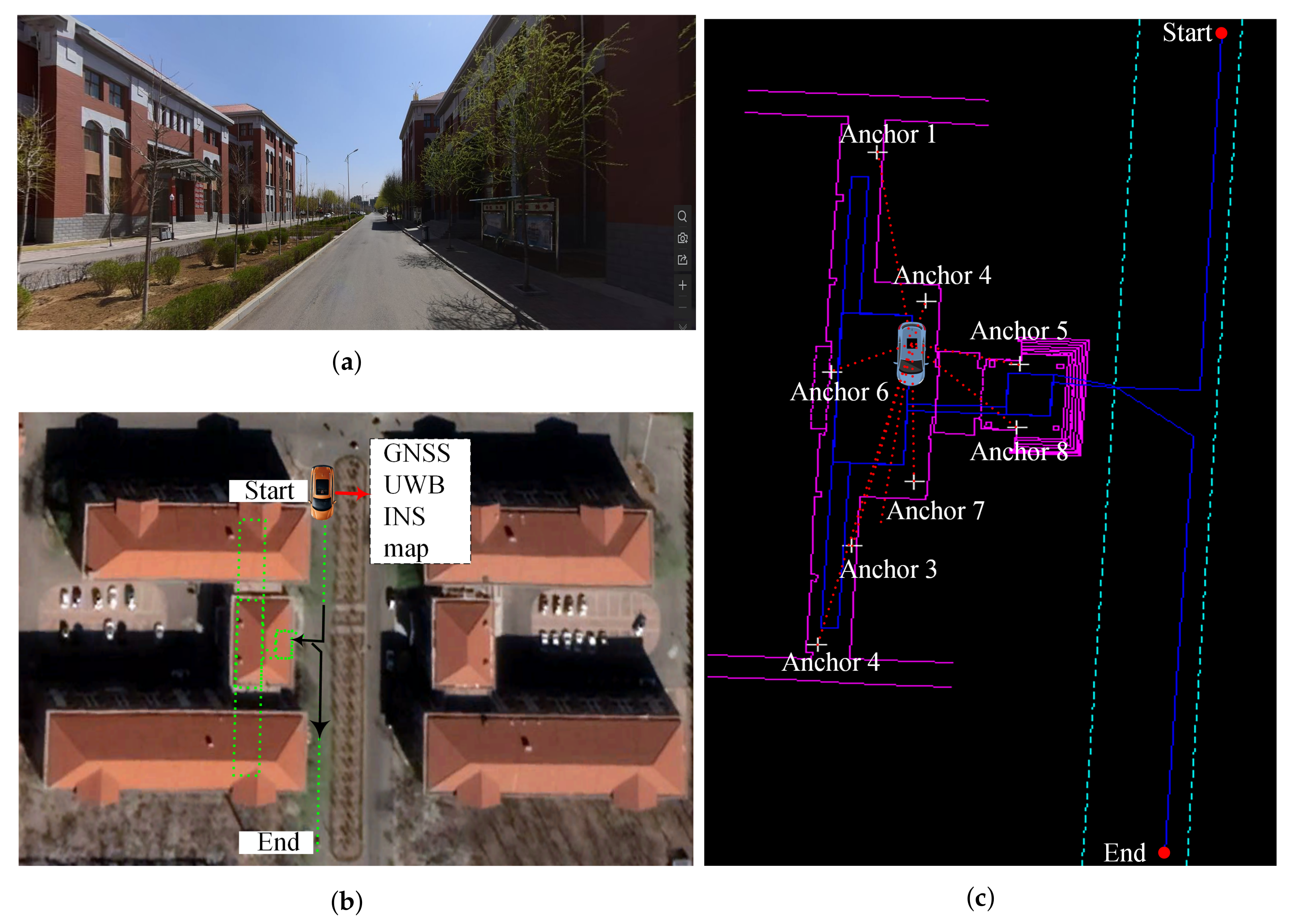
5.1. Experimental Description and Platform Construction

To evaluate the performance of the improved AREKF algorithm based on the proposed TC integrated multi-GNSS-TC RTK/UWB/INS/map system for AV applications, an experimental car was designed to simulate AV driving in complex indoor and outdoor environments. The experimental car is shown in Figure 3a, and the TS50 automatic tracking total station is shown in Figure 3b. Due to the primitiveness of the experimental conditions, the experimental car used in this article is not a perfect AV. For TS50 to effectively track the experimental car and provide an accurate reference trajectory, the speed of the experimental car is approximately 1 m/s, which is much slower than the ideal AVs. In addition, to perform a large amount of data analysis on the transitional environment between indoors and outdoors and the indoor environment, the experiment collects multicircle data along a fixed route in this position. Therefore, the entire experiment time was close to 45 min in a seemingly simple experimental task.

The experimental scene is shown in Figure 4a,b. The selected location is a university campus, where the road is flanked by four-floor buildings on both sides. The experimental layout and the established trajectory are shown in Figure 4c. In Figure 4c, the positions of the UWB anchor nodes are indicated by white plus signs; the start and end tags indicate the start and end positions of the experiment, respectively; and the blue line denotes the established driving trajectory. Because of cost considerations, the layout of the UWB anchor nodes is relatively sparse.

The experimental car was initially aligned with the starting position on the road. After this alignment was completed, the car drove along the road, then drove into an experimental building and continued to follow the experimental trajectory inside the building. After a period of time, the experimental car drove out of the experimental building and proceeded along the road to the end position, at which time the entire experiment was complete. The number of available satellites was severely affected due to obstruction by the buildings, and the satellite signal was strongly influenced by multipath effects. Therefore, the constructed outdoor-transition–indoor-transition–outdoor driving route in a complex environment was sufficient to meet the requirements of the envisaged experiment.

To provide a realistic AV environment, other cars, pedestrians, and experimenters were allowed to pass freely through the experimental area throughout the whole experiment, increasing the difficulty of high-precision AV positioning and the uncertainty during the experiment.

The specifications of the IMU and UWB systems are given in

Table 3. Specifications of the IMU.

Parameter	Accelerometer	Gyroscope
Measurement range	±10 g	±300°/s
Bias stability	25 mGal	1°/h
Random walk	0.1 m/s/$\sqrt{\mathrm{h}}$	0.03°$/\sqrt{\mathrm{h}}$
Sampling frequency	200 Hz	200 Hz

and

Table 4. Specifications of the UWB system.

Parameter	UWB
Ranging principle	TW-TOF
Wave band	3.1–4.8 GHz
Ranging ability	<80 m
LOS accuracy	5 ± 1 cm
NLOS accuracy	Environmentally determined
Sampling frequency	2 Hz

. Tactical-level inertial navigation was applied in this study for the following reasons:

• This article focuses mainly on high-precision positioning systems in pursuit of high precision and continuous reliability of such systems.
• An MEMS IMU was also tested. Although the algorithm proposed in this article improves the positioning accuracy in most environments, the overall positioning accuracy was seriously reduced.

An MEMS IMU currently cannot meet our needs in practical applications. Nevertheless, with the continuous advancement of MEMS IMU technology, our ongoing efforts are dedicated to designing a seamless positioning system that uses an MEMS IMU.

5.2. Time Synchronization and Spatial Unification

In a seamless positioning system, a prerequisite for using a TC integrated multi-GNSS-TC RTK/INS/UWB/map system for an AV is to ensure the unification of the GNSS/INS/UWB time system. Hard time synchronization of the hardware systems is used for the GPST and the INS time to ensure strict time synchronization between the GPS and INS measurements in this paper. Moreover, the times associated with other navigation systems (BDS, Galileo, and GLONASS) are converted to GPST. In addition, the GPS second pulse signal is used to time the computer to ensure that the computer time is strictly synchronized with the GPST. Then, the UWB time is determined based on the computer system time. In this way, the time systems of the UWB, GNSS, and INS measurements are strongly unified. Unfortunately, three issues still exist in the process of time synchronization:

• When GPS is not available, the computer time cannot be corrected by means of the GPS second pulse signal. In this case, the UWB time label depends only on the computer time, which will be subject to clock bias and clock drift after a long time. At present, time-asynchrony error occurrences are shown to exist in experimental observations after several hours, but the impact on the experimental results within a few hours is small.
• The UWB time label obtained using this synchronization method is still affected by the time delay associated with the transmission of the signal to the computer through a universal serial bus (USB) data cable. At present, this delay can be reduced only through calibration technology.
• The sampling frequencies of the GNSS (2 Hz), the INS (200 Hz), and the UWB system (2 Hz) are different. It is necessary to interpolate all observations to correspond to the same observation times to facilitate calculations.

Time synchronization error is a problem that must be solved for high-speed AVs because the faster a vehicle is, the more serious the impact of time synchronization will be. The experimental car used in this work to simulate an AV does not travel very fast (less than 1 m/s), and the time synchronization error is approximately 0.01 s, so the tiny out-of-synchronization error 0.01 s × 1 m/s = 0.01 m (1 cm) can be ignored in this paper.

Spatial synchronization is another prerequisite for using a TC integrated multi-GNSS-TC RTK/INS/UWB/map system for an AV. Figure 5 shows the layout of the experimental platform and the sensor equipment of the experimental car. The experimental platform includes an experimental personal computer (PC), an INS that consists of a three-axis gyroscope and a three-axis accelerometer, a mobile UWB node, and a total reflection prism, which is automatically tracked by a Leica TS50 automatic tracking total station to provide a high-precision trajectory reference for the experimental vehicle. The Leica TS50 automatic tracking total station is also used to establish a station at a control point where the coordinates in the e-frame are known. Thus, the coordinate system for UWB navigation and positioning is unified as the e-frame. Figure 5 shows that all sensors are rigidly connected by an aluminum plate to ensure accurate measurement of the lever arms between different sensors, which are therefore considered to be free of error.

To evaluate the accuracy throughout the entire experiment, the total reflection prism in Figure 5 and the TS50 in Figure 3b were used to provide an experimental reference benchmark. Hence, it was necessary to achieve time synchronization between the reference benchmark provided by the TS50 and the experimental results. As mentioned above, the entire integrated system uses the GPST as the time reference. Since the time of the reference results collected by the TS50 was based on the laptop time, the laptop used for TS50 data reception was also timed based on GPS before data collection to ensure that the reference results also used GPST. The specifications of the TS50 are shown in

Table 5. Specifications of the TS50.

Parameter	TS50
Ranging accuracy	2 mm + 2 ppm
Angle accuracy	0.5″
Sampling frequency	10 Hz

. Due to the high-precision performance of the TS50, the three-dimensional coordinates of the UWB anchor node antennas were also measured using the TS50 and thus are assumed to be free of error.

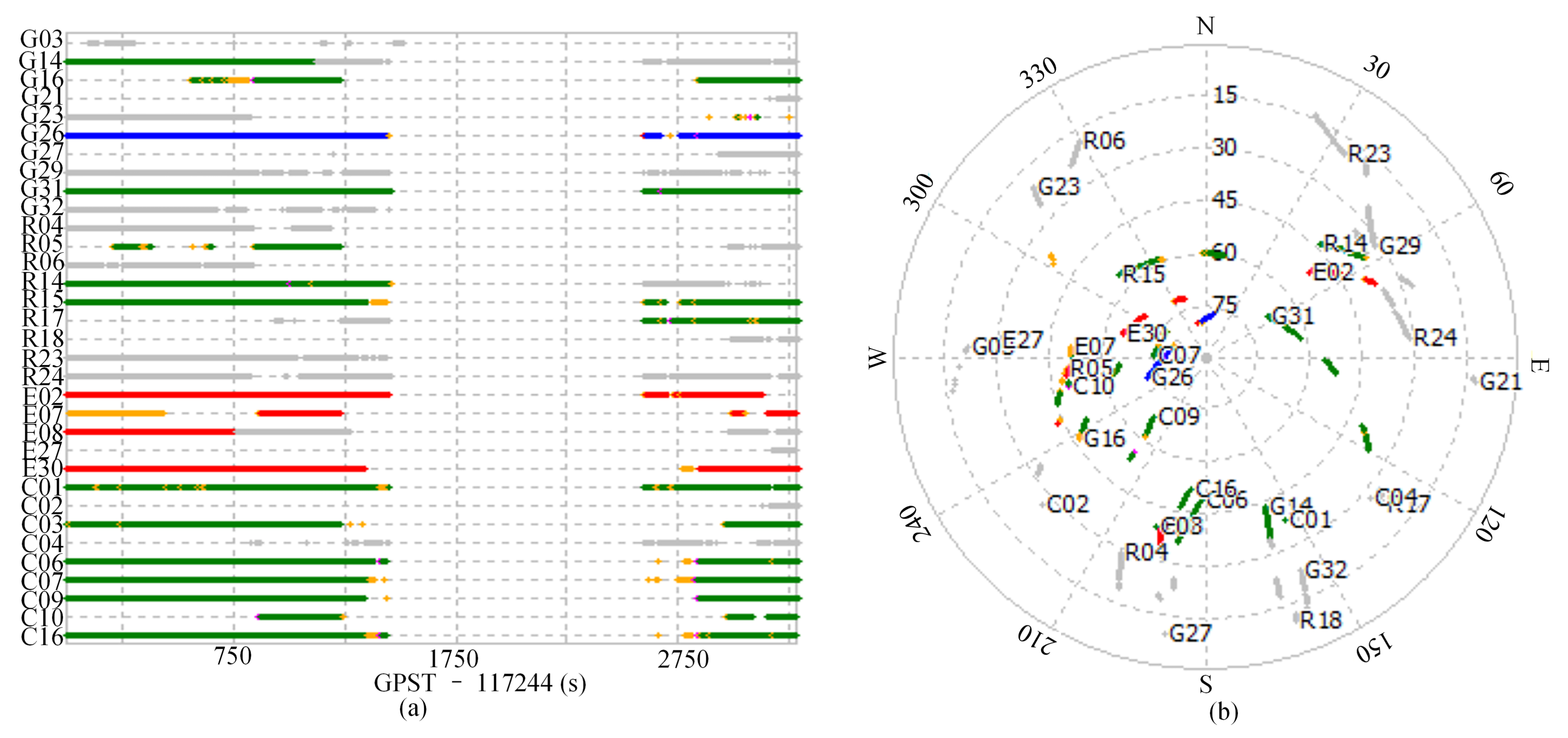
5.3. Satellite Availability

To simulate an extremely dense urban environment and avoid the influence of multipath effects, the cut-off elevation angle in the experiment was set to 35°. Figure 6a,b show the availability of satellites and the starry sky map of the four satellite systems, namely, GPS (G), BDS (C), Galileo (E), and GLONASS (R), with a 35° cut-off elevation angle. Figure 7a shows the number of available satellites in the four satellite systems with a 35° cut-off elevation angle. Figure 7b shows the dilution of precision (DOP) of the four satellite systems with a 35° cut-off elevation angle, including the geometric dilution of precision (GDOP), the position dilution of precision (PDOP), the horizontal dilution of precision (HDOP), and the vertical dilution of precision (VDOP), for the four systems used as the sources of multi-GNSS signals.

It can be seen from Figure 6a and Figure 7a that in the outdoor environment, there are at most four GPS satellites and at most three GLONASS satellites that can be tracked continuously; for Galileo satellites, four can be guaranteed in the early stage, and three in the later stage; and the BDS can guarantee the availability of six to seven satellites. In the transitional environment, the number of available satellites is reduced, with only 5–9 in total among the four systems, and no single satellite system can meet the requirements of high-precision positioning from the perspective of the number of visible satellites. Most satellites make discontinuous observations, and the constellation configuration is poor from the perspectives of satellite visibility analysis and DOP value distribution. Under these conditions, it is beneficial to increase the number of observation equations by using multi-GNSS-TC RTK integration.

It can be seen from Figure 6a and Figure 7 that there is absolutely no GNSS satellite signal for approximately 20 min. At this time, the experimental car simulates AV driving in an indoor environment. Obviously, GNSS positioning can play no role during this period, and thus, only the UWB, INS, and map technologies are used for indoor positioning.

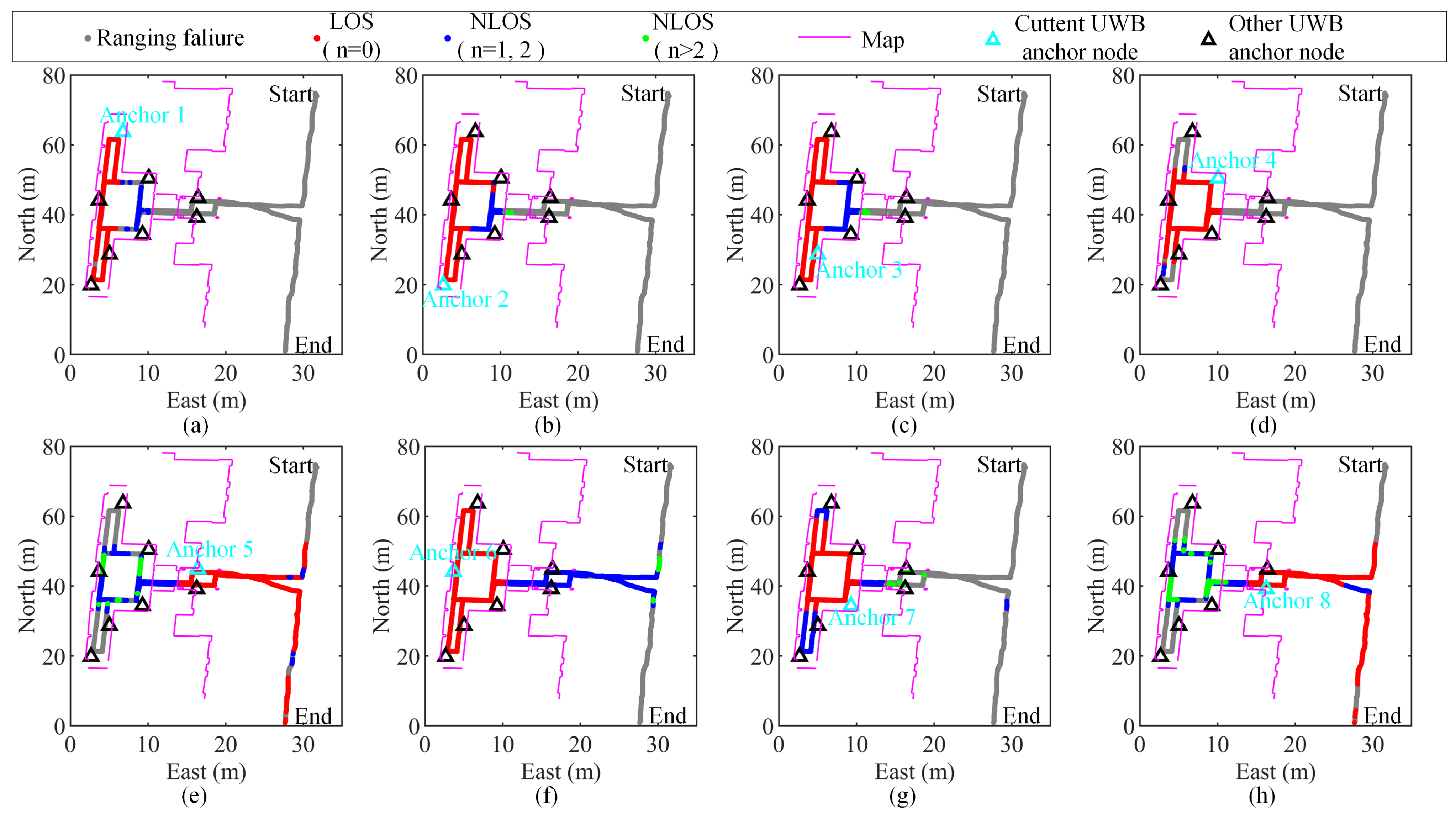
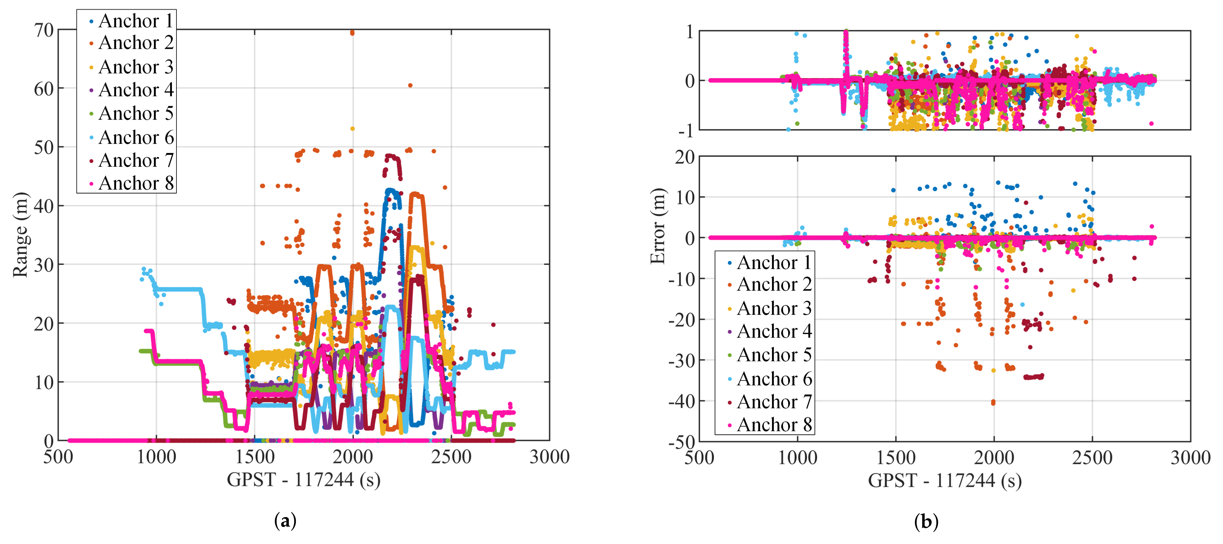
5.4. Influence of the NLOS Error on UWB Measurements

Following the above evaluation of satellite availability, the performance of UWB measurements in the indoor environment and during the transition between the indoor and outdoor environments is analyzed. The ranging statuses of the UWB measurements based on different UWB anchor nodes during the operation of the experimental car are shown in Figure 8. The pink lines represent the known map. The success or failure status of every UWB anchor node on the map and the LOS or NLOS status, as represented by the value of n in Equation (9), at each time are displayed in detail. The time series of the ranging values and errors for the different UWB anchor nodes during the operation of the experimental car are shown in Figure 9. As shown in Figure 8, the environment between the mobile UWB node and the UWB anchor node is usually subject to LOS conditions (indicated by red dots, $n=0$) when successful UWB ranging can be performed. Due to the unique penetration ability of UWB signals, ranging is still possible when this signal is blocked by obstacles, but in this case, the UWB distance measurement value is affected by the obstacles, leading to large errors (indicated by blue or green dots, $n=1,2,3,\dots$) during the operation of the experimental car. When effective UWB ranging cannot be achieved, the UWB signal is usually blocked by multiple walls or fixed facilities on the map. As shown in Figure 9, the UWB ranging error, which is mainly within $1\mathrm{m}$, does not vary with distance. However, many ranging error values exceed tens of meters, mainly due to the NLOS effect of obstacles. Moreover, as shown in Figure 8 and Figure 9, some ranging values are unaffected by obstacles but still exhibit large errors because the UWB signal is interfered with by the surrounding environment.

Therefore, the method of identifying and eliminating NLOS errors based on UWB/INS/map integration proposed in Section 3.2 was used to adjust the weights of the UWB measurement values affected by NLOS errors. Then, to address the ranging values associated with the UWB signals interfered with by the surrounding environment, the improved AREKF algorithm proposed in Section 4.2 was applied to resist the influence of these abnormal UWB measurement values.

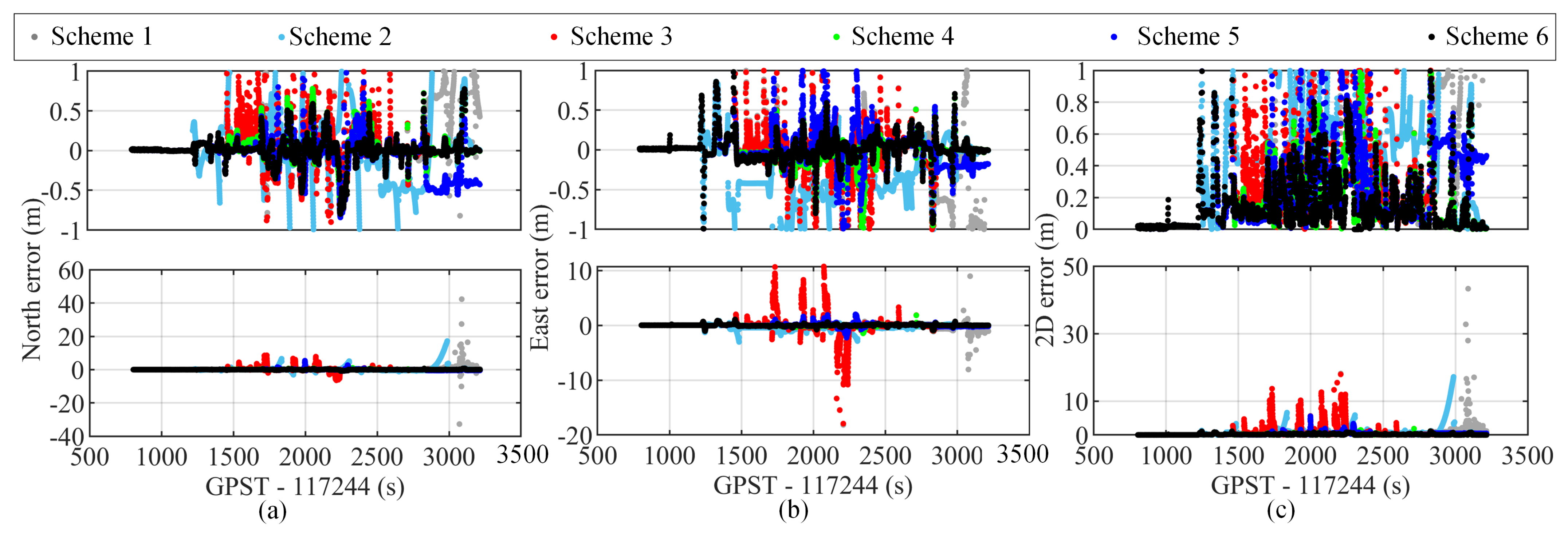
5.5. Analysis of the Positioning Results

To evaluate the improved AREKF algorithm based on the single-frequency TC integrated multi-GNSS-TC RTK/UWB/INS/map system proposed in this article, six schemes were designed and compared:

• Scheme 1: The EKF algorithm based on the single-frequency TC integrated multi-GNSS RTK/UWB/INS system.
• Scheme 2: The EKF algorithm based on the single-frequency TC integrated multi-GNSS-TC RTK/INS system.
• Scheme 3: The EKF algorithm based on the single-frequency TC integrated multi-GNSS-TC RTK/UWB/INS system.
• Scheme 4: The improved AREKF algorithm based on the single-frequency TC integrated multi-GNSS-TC RTK/UWB/INS system.
• Scheme 5: The EKF algorithm based on the single-frequency TC integrated multi-GNSS-TC RTK/UWB/INS/map system.
• Scheme 6: The improved AREKF algorithm based on the single-frequency TC integrated multi-GNSS-TC RTK/UWB/INS/map system (the method proposed in this paper).

The effectiveness of multi-GNSS-TC can be verified by comparing Scheme 1 with other schemes. The effectiveness of increasing the sensor UWB can be verified by comparing Scheme 2 and other schemes. The effectiveness of the improved AREKF algorithm can be verified by comparing Schemes 3 and 4. The importance of the map can be verified by comparing Schemes 3 and 5. Scheme 6 verifies the effectiveness and feasibility of the positioning scheme for AVs proposed in this article.

The complete trajectories and CDF of the positioning errors under each of the six schemes are shown in Figure 10. The positioning error results of the different schemes are further compared in

Table 6. Comparison of the RMS accuracies, average and maximum errors, and ambiguity fixing rates under the different schemes.

		Scheme 1	Scheme 2	Scheme 3	Scheme 4	Scheme 5	Scheme 6
RMS (m)	North	1.6405	2.0621	1.0365	0.2593	0.3526	0.1756
	East	1.8507	0.6411	1.8118	0.2795	0.3653	0.1698
	2D	2.4731	2.1594	2.0873	0.3565	0.5077	0.2443
Average (m)	North	0.5583	0.7172	0.4247	0.1672	0.1645	0.0932
	East	0.7539	0.4503	0.6916	0.1805	0.2154	0.1049
	2D	1.0377	0.9919	0.8848	0.2530	0.3105	0.1657
Max (m)	North	42.3682	17.2070	8.6099	0.9990	5.4026	0.7986
	East	18.1621	3.0340	17.9310	1.8241	2.2516	1.0632
	2D	43.3052	17.2074	17.9450	1.8464	5.5461	1.1372
Fixing rate (%)		54.6	68.4	78.5	83.2	79.7	89.4

.

In the initial stage in the outdoor environment, because the experiment had just started and the inertial navigation accuracy was high without divergence, the accuracy of several schemes was relatively high.

In the transitional environment between indoors and outdoors, the numbers of available GNSS and UWB observations were small, and these observations were affected by the environment, leading to greater noise. In Schemes 1 and 3, no processing is performed on the GNSS and UWB observations and, consequently, the positioning results severely diverge under these schemes. In Schemes 2, 3, 4, 5, and 6, multi-GNSS-TC is used to improve the success rate of ambiguity resolution. Schemes 2, 3, 4, 5, and 6 all effectively take measures to process the observations to varying degrees, and the positioning accuracy under these schemes is obviously higher than that under Scheme 1. In Scheme 4, the improved AREKF algorithm is used to adjust the weights of GNSS and UWB observations and prevent excessive convergence of the filtering state. Scheme 5 uses a map to identify and eliminate NLOS errors in the UWB observations. In Scheme 6, a map is used to identify and eliminate UWB NLOS errors, and then the improved AREKF algorithm is used to adjust the weights of GNSS and UWB observations to reduce the influence of other outliers due to multipath effects, signal interference, and other errors. Moreover, the improved AREKF algorithm effectively prevents any abnormal filtering status.

In the indoor environment stage, the UWB observations had not been cleaned, so there were no good UWB observations available for Schemes 1 and 3, and the corresponding positioning accuracy was very poor, especially at the corners of the rectangular corridor (near UWB anchor nodes 1 and 4). Scheme 2 has no UWB data, the position begins to diverge gradually, and the positioning error gradually becomes larger. Scheme 4 uses the improved AREKF algorithm to process UWB noise; consequently, the positioning trajectory was relatively smooth, but the accuracy at the corners of the corridor was still poor. Scheme 5 uses a map to identify and eliminate UWB NLOS errors, and the positioning results do not show a large amount of divergence, but the accuracy at the corners was also poor. Scheme 6 uses both a map and the improved AREKF algorithm to effectively solve the problem of difficult positioning at indoor corners; thus, the solution result was closer to the reference trajectory.

From the time when the experimental car exited the building until the end stage, fewer satellite observation equations were available for Scheme 1, and the ambiguity could not be successfully fixed, resulting in poor accuracy. Scheme 2 can only rely on the INS in the indoor phase, the position divergence is serious, and the ambiguity cannot be fixed immediately when the number of satellites is small. Comparing Schemes 2, 3, 4, 5, and 6, it can be seen that in the final stage of the outdoor environment, several of the schemes adopt multi-GNSS-TC RTK, which significantly improves the ambiguity-fixed rate to varying degrees.

However, it can be seen from Figure 10 that in the outdoor stage, the solution trajectories of Schemes 3 and 5 were not completely consistent with the reference trajectory, Scheme 2 still had a large position error when it just entered the outdoor stage, Scheme 4 was relatively consistent, and Scheme 6 was very consistent with the reference trajectory. The reason for the large error in Scheme 2 is that when the experimental car had just exited the room, the entire system of Scheme 2 could rely only on INS mechanization for nearly 30 min. At this time, the accuracy of the floating-point solution of Scheme 2 was very poor, GNSS data quality was poor, and there were few GNSS satellites available. The ambiguity resolution could not be fixed, the accuracy of the floating-point solution could not be improved immediately, and the inertial navigation error parameters were not accurately estimated. Therefore, this part of the results for Scheme 2 is even worse than the results of Scheme 1. In schemes other than Scheme 2, UWB observations were still available, and the corresponding accuracy was better than that of Scheme 2. The reason for this phenomenon is that the accuracy of the floating-point solution in the transition environment affects the ambiguity-fixed and the accuracy of the solution. In the transitional environment, Scheme 6 uses the map to process NLOS, uses the improved AREKF algorithm to adjust the noise matrix at the same time to adjust the weight of the observation value of GNSS and UWB, effectively preventing the abnormal filtering state, and then uses multi-GNSS-TC RTK to effectively control the accuracy of floating-point solutions in the outdoor environment. Therefore, both Schemes 4 and 6 use the improved AREKF algorithm and multi-GNSS-TC RTK in an outdoor environment, and Scheme 6 has a better ambiguity-fixed success rate and accuracy than those of Scheme 4.

The positioning errors under the different schemes in various directions are compared in Figure 11. To facilitate analysis, each subfigure includes an enlarged view to show the details in Figure 11. The errors under Schemes 1, 2, and 3 can be up to tens of meters, and those under Schemes 4 and 5 often exceed $1\mathrm{m}$, while the errors under Scheme 6 can basically be controlled within $1\mathrm{m}$, which is sufficient to guarantee the safety and stability of an AV.

Based on Figure 10 and Figure 11, Table 6, and the analysis above, a comparison of Schemes 1 and 3 reveals that using multi-GNSS-TC RTK can significantly improve the success rate of ambiguity resolution and the positioning accuracy. A comparison of Schemes 2, 3, 4, and 5 indicates that increasing the UWB sensor and processing the UWB observations are very important. As seen by comparing Schemes 3 and 4, the positioning accuracy is significantly increased when the improved AREKF algorithm is used to adjust the weights of the observation values, and the smoothness and stability of the positioning trajectory are enhanced. A comparison of Schemes 3 and 5 indicates that the introduction of map information under the same conditions as in the other experimental settings significantly improves the positioning accuracy in both the indoor environment and the transitional environment between indoors and outdoors, which shows that the use of map information, as proposed in this article, is effective in identifying and reducing UWB NLOS errors. In Scheme 6, the improved AREKF algorithm based on a single-frequency TC integrated multi-GNSS-TC RTK/UWB/INS/map system is used at the same time. Regardless of the environment (outdoor, transitional, or indoor), the root mean square (RMS) accuracies in the north, east, and 2D directions are 0.1756 m, 0.1698 m, and 0.2443 m, respectively; the average errors in the north, east, and 2D directions are 0.0932 m, 0.1049 m, and 0.1657 m, respectively; and the maximum errors in the north, east, and 2D directions are 0.7986 m, 1.0632 m, and 1.1372 m, respectively. The ambiguity-fixed rate can reach 89.4%. Thus, the positioning accuracy and stability of the strategy and algorithm of Scheme 6 are significantly higher than those of the other schemes, sufficient to guarantee high precision, safety, and stability for an AV.

6. Conclusions

The high-precision positioning of AVs in a seamless environment is still a challenging problem. In this study, an improved AREKF algorithm based on a single-frequency TC integrated multi-GNSS-TC RTK/UWB/INS/map system is developed to provide reliable, continuous, and high-precision positioning in challenging seamless indoor/outdoor environments. Multi-GNSS-TC RTK and INS measurements are used to address the limited number of available satellites in the outdoor environment and improve the ambiguity-fixed rate. In addition, UWB technology is used in place of GNSS signals to provide effective observations in GNSS-challenged or indoor environments. However, UWB observations are seriously affected by NLOS errors. Hence, map and INS information are used to identify and eliminate the effects of UWB NLOS errors. Additionally, to weaken the influence of multipath effects or outliers due to environmental interference in GNSS and UWB observations, an improved AREKF algorithm is proposed that can effectively resist the influence of outliers and abnormal filtering statuses. Experimental results show that the RMS accuracies of the proposed algorithm and system in the north, east, and 2D directions are 0.1756 m, 0.1698 m, and 0.2443 m, respectively; the average errors in the north, east, and 2D directions are 0.0932 m, 0.1049 m, and 0.1657 m, respectively; and the maximum errors in the north, east, and 2D directions are 0.7986 m, 1.0632 m, and 1.1372 m, respectively. The ambiguity-fixed rate can reach 89.4%. Whether in outdoor, transitional, or indoor environments, the positioning accuracy and stability of the proposed solution are significantly higher than those of other schemes, which is sufficient to guarantee high positioning accuracy, safety, and stability for AVs.

Although the proposed scheme achieves some progress in AV positioning, the maximum error is still close to 1 m. To make the AV positioning system more reliable, other auxiliary sensors, such as LiDAR and cameras, will be considered in the future to further enhance the positioning stability, improve high-precision capabilities, and avoid major accidents.

References

1. Li, J.; Cui, X.; Li, Z.; Liu, J. Method to improve the positioning accuracy of vehicular nodes using IEEE 802.11p protocol. IEEE Access 2017, 6, 2834–2843. [Google Scholar] [CrossRef]
2. Ren, K.; Wang, Q.; Wang, C.; Qin, Z.; Lin, X. The security of autonomous driving: Threats, defenses, and future directions. Proc. IEEE 2019, 108, 357–372. [Google Scholar] [CrossRef]
3. Liu, S.; Liu, L.; Tang, J.; Yu, B.; Wang, Y.; Shi, W. Edge computing for autonomous driving: Opportunities and challenges. Proc. IEEE 2019, 107, 1697–1716. [Google Scholar] [CrossRef]
4. Jonasson, M.; Rogenfelt, Å.; Lanfelt, C.; Fredriksson, J.; Hassel, M. Inertial navigation and position uncertainty during a blind safe stop of an autonomous vehicle. IEEE Trans. Veh. Technol. 2020, 69, 4788–4802. [Google Scholar] [CrossRef]
5. Xiong, H.; Mai, Z.; Tang, J.; He, F. Robust GPS/INS/DVL navigation and positioning method using adaptive federated strong tracking filter based on weighted least square principle. IEEE Access 2019, 7, 26168–26178. [Google Scholar] [CrossRef]
6. Li, T.; Zhang, H.; Gao, Z.; Chen, Q.; Niu, X. High-accuracy positioning in urban environments using single-frequency multi-GNSS RTK/MEMS-IMU integration. Remote Sens. 2018, 10, 205. [Google Scholar] [CrossRef] [Green Version]
7. Hao, Y.; Xu, A.; Sui, X.; Wang, Y. A modified extended Kalman filter for a two-antenna GPS/INS vehicular navigation system. Sensors 2018, 18, 3809. [Google Scholar] [CrossRef] [PubMed] [Green Version]
8. Mur-Artal, R.; Tardós, J.D. ORB-SLAM2: An open-source SLAM system for monocular, stereo, and RGB-D cameras. IEEE Trans. Robot. 2017, 33, 1255–1262. [Google Scholar] [CrossRef] [Green Version]
9. Davison, A.J.; Reid, I.D.; Molton, N.D.; Stasse, O. MonoSLAM: Real-Time single camera SLAM. IEEE Trans. Pattern. Anal. Mach. Intell. 2007, 29, 1052–1067. [Google Scholar] [CrossRef] [PubMed] [Green Version]
10. Dill, E.; de Haag, M.U.; Duan, P.; Serrano, D.; Vilardaga, S. Seamless indoor-outdoor navigation for unmanned multi-sensor aerial platforms. In Proceedings of the 2014 IEEE/ION Position, Location and Navigation Symposium (PLANS 2014), Monterey, CA, USA, 5–8 May 2014. [Google Scholar]
11. Tao, X.; Zhang, X.; Zhu, F.; Wang, F.; Teng, W. Precise displacement estimation from time-differenced carrier phase to improve PDR performance. IEEE Sens. J. 2018, 18, 8238–8246. [Google Scholar] [CrossRef]
12. Niu, X.; Liu, T.; Kuang, J.; Li, Y. A Novel Position and Orientation System for Pedestrian Indoor Mobile Mapping System. IEEE Sens. J. 2021, 21, 2104–2114. [Google Scholar] [CrossRef]
13. Cheng, J.; Yang, L.; Li, Y.; Zhang, W. Seamless outdoor/indoor navigation with WIFI/GPS aided low cost Inertial Navigation System. Phys. Commun. 2014, 13, 31–43. [Google Scholar] [CrossRef]
14. Huang, H.; Zeng, Q.; Chen, R.; Meng, Q.; Wang, J.; Zeng, S. Seamless navigation methodology optimized for indoor/outdoor detection based on wifi. In Proceedings of the 2018 Ubiquitous Positioning, Indoor Navigation and Location-Based Services (UPINLBS), Wuhan, China, 22–23 March 2018. [Google Scholar]
15. Zhang, X.; Zeng, Q.; Meng, Q.; Xiong, Z.; Qian, W. Design and realization of a mobile seamless navigation and positioning system based on Bluetooth technology. In Proceedings of the 2016 IEEE Chinese Guidance, Navigation and Control Conference (CGNCC), Nanjing, China, 12–14 August 2016. [Google Scholar]
16. Silva, B.; Hancke, G.P. IR-UWB-based non-line-of-sight identification in harsh environments: Principles and challenges. IEEE Trans. Industr. Inform. 2016, 12, 1188–1195. [Google Scholar] [CrossRef]
17. Adebomehin, A.A.; Walker, S.D. Enhanced Ultrawideband methods for 5G LOS sufficient positioning and mitigation. In Proceedings of the 2016 IEEE 17th International Symposium on A World of Wireless, Mobile and Multimedia Networks (WoWMoM), Coimbra, Portugal, 21–24 June 2016. [Google Scholar]
18. Rizos, C.; Roberts, G.; Barnes, J.; Gambale, N. Experimental results of Locata: A high accuracy indoor positioning system. In Proceedings of the 2010 International Conference on Indoor Positioning and Indoor Navigation (IPIN), Zurich, Switzerland, 15–17 September 2010. [Google Scholar]
19. Chen, X.; Xu, Y.; Li, Q.; Tang, J.; Shen, C. Improving ultrasonic-based seamless navigation for indoor mobile robots utilizing EKF and LS-SVM. Measurement 2016, 92, 243–251. [Google Scholar] [CrossRef]
20. Liu, T.; Niu, X.; Kuang, J.; Cao, S.; Zhang, L.; Chen, X. Doppler shift mitigation in acoustic positioning based on pedestrian dead reckoning for smartphone. IEEE Trans. Instrum. Meas. 2020, 70. [Google Scholar] [CrossRef]
21. Pietra, D.V.; Dabove, P.; Piras, M. Seamless Navigation using UWB-based Multisensor System. In Proceedings of the 2020 IEEE/ION Position, Location and Navigation Symposium (PLANS), Portland, OR, USA, 20–23 April 2020. [Google Scholar]
22. Odolinski, R.; Teunissen, P.J.G.; Odijk, D. Combined BDS, Galileo, QZSS and GPS single-frequency RTK. GPS Solut. 2015, 19, 151–163. [Google Scholar] [CrossRef]
23. Odijk, D.; Nadarajah, N.; Zaminpardaz, S.; Teunissen, P.J.G. GPS, Galileo, QZSS and IRNSS differential ISBs: Estimation and application. GPS Solut. 2017, 21, 439–450. [Google Scholar] [CrossRef]
24. Liu, Y.; Liu, F.; Gao, Y.; Zhao, L. Implementation and analysis of tightly coupled global navigation satellite system precise point positioning/inertial navigation system (GNSS PPP/INS) with insufficient satellites for land vehicle navigation. Sensors 2018, 18, 4305. [Google Scholar] [CrossRef] [PubMed] [Green Version]
25. Chiang, K.W.; Chang, H.W.; Li, Y.H.; Tsai, G.J.; Tseng, C.L.; Tien, Y.C.; Hsu, P.C. Assessment for ins/gnss/odometer/barometer integration in loosely-coupled and tightly-coupled scheme in a gnss-degraded environment. IEEE Sens. J. 2019, 20, 3057–3069. [Google Scholar] [CrossRef]
26. Liu, Y.; Fan, X.; Lv, C.; Wu, J.; Li, L.; Ding, D. An innovative information fusion method with adaptive Kalman filter for integrated INS/GPS navigation of autonomous vehicles. Mech. Syst. Signal Process. 2018, 100, 605–616. [Google Scholar] [CrossRef] [Green Version]
27. Li, X.; Wang, Y.; Khoshelham, K. A robust and adaptive complementary kalman filter based on Mahalanobis distance for Ultra Wideband/Inertial Measurement Unit fusion positioning. Sensors 2018, 18, 3435. [Google Scholar] [CrossRef] [Green Version]
28. Groves, P.D. Principles of GNSS, inertial, and multi-sensor integrated navigation systems. IEEE Aero. El. Sys. Mag. 2015, 30, 26–27. [Google Scholar] [CrossRef]
29. Liu, F.; Wang, J.; Zhang, J.; Han, H. An indoor localization method for pedestrians base on combined UWB/PDR/Floor Map. Sensors 2019, 19, 2578. [Google Scholar] [CrossRef] [Green Version]
30. Qian, J.; Ma, J.; Ying, R.; Liu, P.; Pei, L. An improved indoor localization method using smartphone inertial sensors. In Proceedings of the International Conference on Indoor Positioning and Indoor Navigation, Montbeliard, Belfort, France, 28–21 October 2013. [Google Scholar]
31. Lan, K.C.; Shih, W.Y. On calibrating the sensor errors of a PDR-based indoor localization system. Sensors 2013, 13, 4781–4810. [Google Scholar] [CrossRef] [Green Version]
32. Shin, E.H. Estimation Techniques for Low-Cost Inertial Navigation. Ph.D. Thesis, University of Calgary, Calgary, AB, Canada, 2005. [Google Scholar]
33. Benson, D.O. A Comparison of Two Approaches to Pure-Inertial and Doppler-Inertial Error Analysis. IEEE Trans. Aero. Elec. Syst. 1975, AES-11, 447–455. [Google Scholar] [CrossRef]
34. Park, M. Error Analysis and Stochastic Modeling of MEMS Based Inertial Sensors for Land Vehicle Navigation Applications. Ph.D. Thesis, University of Calgary, Calgary, AB, Canada, April 2004. [Google Scholar]
35. Wang, C.; Xu, A.; Kuang, J.; Sui, X.; Hao, Y.; Niu, X. A High-Accuracy Indoor Localization System and Applications Based on Tightly Coupled UWB/INS/Floor Map Integration. IEEE Sens. J. 2021, 21, 18166–18177. [Google Scholar] [CrossRef]
36. Li, M. Research on Multi-GNS S Precise Orbit Determination Theory and Application. Ph.D. Thesis, Wuhan University, Wuhan, China, April 2011. [Google Scholar]
37. Sui, X. Research on the Theory and Method of Inter-System Double Difference Ambiguity Forming and Fixing for Multi-GNSS. Ph.D. Thesis, Wuhan University, Wuhan, China, May 2017. [Google Scholar]
38. Blewitt, G. Carrier phase ambiguity resolution for the Global Positioning System applied to geodetic baselines up to 2000 km. J. Geophys. Res. Atmos. 1989, 94, 10187–10203. [Google Scholar] [CrossRef] [Green Version]
39. Yang, Y.; Song, L.; Xu, T. Robust estimator for correlated observations based on bifactor equivalent weights. J. Geod. 2002, 76, 353–358. [Google Scholar] [CrossRef]
40. Yan, G.; Deng, Y. Review on Practical Kalman Filtering Techniques in Traditional Integrated Navigation System. Navig. Position. Timing 2020, 7, 50–64. [Google Scholar]
Figure 1. NLOS identification.
Remotesensing 14 00027 g001
Figure 2. Algorithm flowchart.
Remotesensing 14 00027 g002
Figure 3. Experimental car and automatic tracking total station. (a) Experimental car. (b) Leica TS50 automatic tracking total station.
Remotesensing 14 00027 g003
Figure 4. Experimental scene and design. (a) Experimental environment. (b) Top view of the experimental scene and the designed trajectory. (c) Experimental layout and established trajectory.
Remotesensing 14 00027 g004
Figure 5. Experimental platform and sensor layout.
Remotesensing 14 00027 g005
Figure 6. Satellite availability in a dense urban environment with a 35° cut-off elevation angle. (a) Satellite availability. (b) Starry sky map of satellites.
Remotesensing 14 00027 g006
Figure 7. Number of available satellites and DOP for the multi-GNSS scenario with a 35° cut-off elevation angle. (a) Number of satellites. (b) DOP.
Remotesensing 14 00027 g007
Figure 8. Occlusion status on the map for different UWB anchor nodes: (a) anchor node 1; (b) anchor node 2; (c) anchor node 3; (d) anchor node 4; (e) anchor node 5; (f) anchor node 6; (g) anchor node 7; (h) anchor node 8. The light blue and black triangles indicate the positions of the current UWB anchor node and other UWB anchor nodes, respectively. The dots of different colors represent various occlusion states of the current UWB anchor node (including ranging failure, LOS conditions, and NLOS conditions).
Remotesensing 14 00027 g008
Figure 9. Time series of the ranging values and errors for different UWB anchor nodes. (a) Ranging values. (b) Errors.
Remotesensing 14 00027 g009
Figure 10. Experimental results under different schemes. (a) Positioning trajectory results. (b) CDF of the positioning errors.
Remotesensing 14 00027 g010
Figure 11. Comparison of the positioning errors under different schemes. (a) North. (b) East. (c) Plane.
Remotesensing 14 00027 g011