Forward-Looking Super-Resolution Imaging for Sea-Surface Target with Multi-Prior Bayesian Method

Abstract

Traditional forward-looking super-resolution methods mainly concentrate on enhancing the resolution with ground clutter or no clutter scenes. However, sea clutter exists in the sea-surface target imaging, as well as ground clutter when the imaging scene is a seacoast.Meanwhile, restoring the contour information of the target has an important effect, for example, in the autonomous landing on a ship. This paper aims to realize the forward-looking imaging of a sea-surface target. In this paper, a multi-prior Bayesian method, which considers the environment and fuses the contour information and the sparsity of the sea-surface target, is proposed. Firstly, due to the imaging environment in which more than one kind of clutter exists, we introduce the Gaussian mixture model (GMM) as the prior information to describe the interference of the clutter and noise. Secondly, we fuse the total variation (TV) prior and Laplace prior, and propose a multi-prior to model the contour information and sparsity of the target. Third, we introduce the latent variable to simplify the logarithm likelihood function. Finally, to solve the optimal parameters, the maximum posterior-expectation maximization (MAP-EM) method is utilized. Experimental results illustrate that the multi-prior Bayesian method can enhance the azimuth resolution, and preserve the contour information of the sea-surface target.

1. Introduction

Scanning radar works as a non-coherent sensor and can be suitable for any geometry situation. Therefore, the scanning radar can be employed in many applications, such as forward-looking imaging [1,2,3,4]. In surveillance, reconnaissance, or situation awareness, high resolution is critical for forward-looking imaging. The range resolution after pulse compression is written as

$${\rho }_r=c/2B_r$$

(1)

where c is the light speed, and $B_r$ is the bandwidth. Scanning radar commonly transmits the linear frequency modulated (LFM) signal with a wide bandwidth to improve the range resolution [5,6]. In the azimuth direction, the resolution is written as

$${\rho }_a=R·\left(\lambda /D\right)$$

(2)

where R denotes the range, $\lambda$ denotes the wavelength, and D denotes the size of the antenna aperture. In theory, we can increase the size of the antenna aperture to enhance the angular resolution [7,8,9]. However, it is infeasible due to the practical limitation. Therefore, low angular resolution hinders the forward-looking imaging quality in practical applications.

Many works suggest that the azimuth echo signal can be seen as a convolution form between the antenna pattern and the target scattering coefficient. The angular resolution can be increased by deconvolution or inverse filtering operations [10,11,12]. Unfortunately, the antenna pattern is a low pass filter. In deconvolution procession, the noise amplitude in high frequency will be amplified to affect the azimuth resolution. Therefore, the direct deconvolution procession is an ill-posed problem.

To alleviate the ill-posed problem, the super-resolution methods are introduced [13,14,15,16,17]. The regularized methods which add different prior terms to the objective function are a main class of super-resolution methods [18,19]. The truncated singular value decomposition (TSVD) method is adopted to improve the resolution by discarding the small singular value components [20]. However, this method losses some information and has a low improvement in azimuth resolution. In [21], the authors introduce the Tikhonov regularization to depress the noise. However, this method smooths the processed result, and the azimuth resolution is not much improved. In the past years, the spectral estimation methods are utilized to increase the azimuth resolution [22,23]. Iterative adaptive approach (IAA) and its improved method are applied for forward-looking imaging [16,24]. The IAA method has a good behavior to depress the noise and improve the azimuth resolution, while the computational complexity is high. To denoise and regularize sparse data, a multichannel spectral analysis method is proposed in [25]. This method uses the $L_2$ norm and the covariance matrices associated with data for denoising and reconstructing sparse signals with the aid of additional information. At the same time, the Bayesian estimation methods are utilized by maximum a posteriori (MAP) to improve the azimuth resolution [26,27]. In the Bayesian methods, the prior information of the imaging system is crucial [28,29]. Poisson distribution is considered as the prior statistical model of the noise and targets’ scattering [30].

In the imaging region, the interest targets usually have some prior information, such as sparsity and contour information. Compared with the entire imaging area, the targets would be sparse in ship monitoring or airport surveillance. To reconstruct the sparse characteristic, the sparse regularization method is applied by selecting reasonable prior information. In [31], the authors add an $L_p$ norm term to the objective function to reconstruct the sparse target. In [32,33], the authors use $L_1$ norm to reconstruct the sparse target of the imaging area. The authors propose a sparse spectral estimation method named sparse iterative covariance-based estimation (SPICE) in [34]. Then, SPICE and $q-$ SPICE methods are applied for scanning radar imaging in [17,35], and the reconstruction result of the targets is significant. In Bayesian methods, the Laplace prior distribution is commonly chosen as the statistical model for the prior information of the sparse targets [36,37,38]. In some applications, we intend to get the precise contour information of the target, such as in autopilot or autonomous landing of aircraft. Therefore, obtaining the contour information of the target is one of main purposes of forward-looking imaging. The TV regularization is usually used to highlight the contour information by minimizing the difference value between adjacent points in the image procession region [39]. In [40,41], the authors introduce the TV prior to estimate the target in forward-looking imaging, and the performance is significant.

For sea-surface monitoring, the prior information of the imaging environment also requires attention. When the imaging scene is the sea-surface, sea clutter would influence the quality of the reconstruction result. In [42], the authors attempted to use the full-polarization method to deal with the detection of small floating target on sea-surface. By using the full-polarization information to detect sea-surface target, the information received by radar can be fully used, and the detection performance is effective. Computer vision combined with image processing technology is introduced to realize the sea-surface monitoring in recent years. Liu at al. [43] show that the sea-surface target detection based on improved YOLOv3 has high accuracy. In forward-looking imaging, Zhang et al. [44] use the Rayleigh distribution to model the sea clutter. At the seacoast, the ground clutter and the sea clutter will influence the reconstruction result together. A single clutter distribution is insufficient to characterize the clutter in this scenario. In [45], to characterize the interference of the clutter and noise, the GMM is introduced. However, this method does not do well at preserving the contour information.

In this paper, we propose a multi-prior Bayesian method which considers the imaging environment and fuses the sparsity and the contour information of the sea-surface target. Firstly, we utilize GMM to describe the interference since we assume the interference distribution is constructed from various simple Gaussian distributions. Subsequently, by adjusting the means, variances, and the mixing coefficient of Gaussian distributions, the interference model gets more flexible to describe the clutter and noise. Secondly, we propose a multi-prior distribution to express the target via fusing the Laplace prior and the TV prior. By adjusting the weighted parameters of the Laplace prior and the TV prior, the multi-prior not only describes the sparsity of the target but also preserves the contour information. Third, we introduce the latent variable to simplify the logarithm likelihood function. Finally, we estimate the parameters by introducing the MAP-EM method.

The article is organized as follows. In Section 2, we analyze the azimuth signal model. In Section 2, we propose a multi-prior Bayesian model for sea-surface target to estimate the imaging parameters. In Section 3, several experiments are shown to verify the effectiveness of the multi-prior Bayesian method. In Section 4, we discuss the shortcoming and the future research directions of the multi-prior Bayesian method. Finally, the conclusions are drawn in Section 5.

2. Method

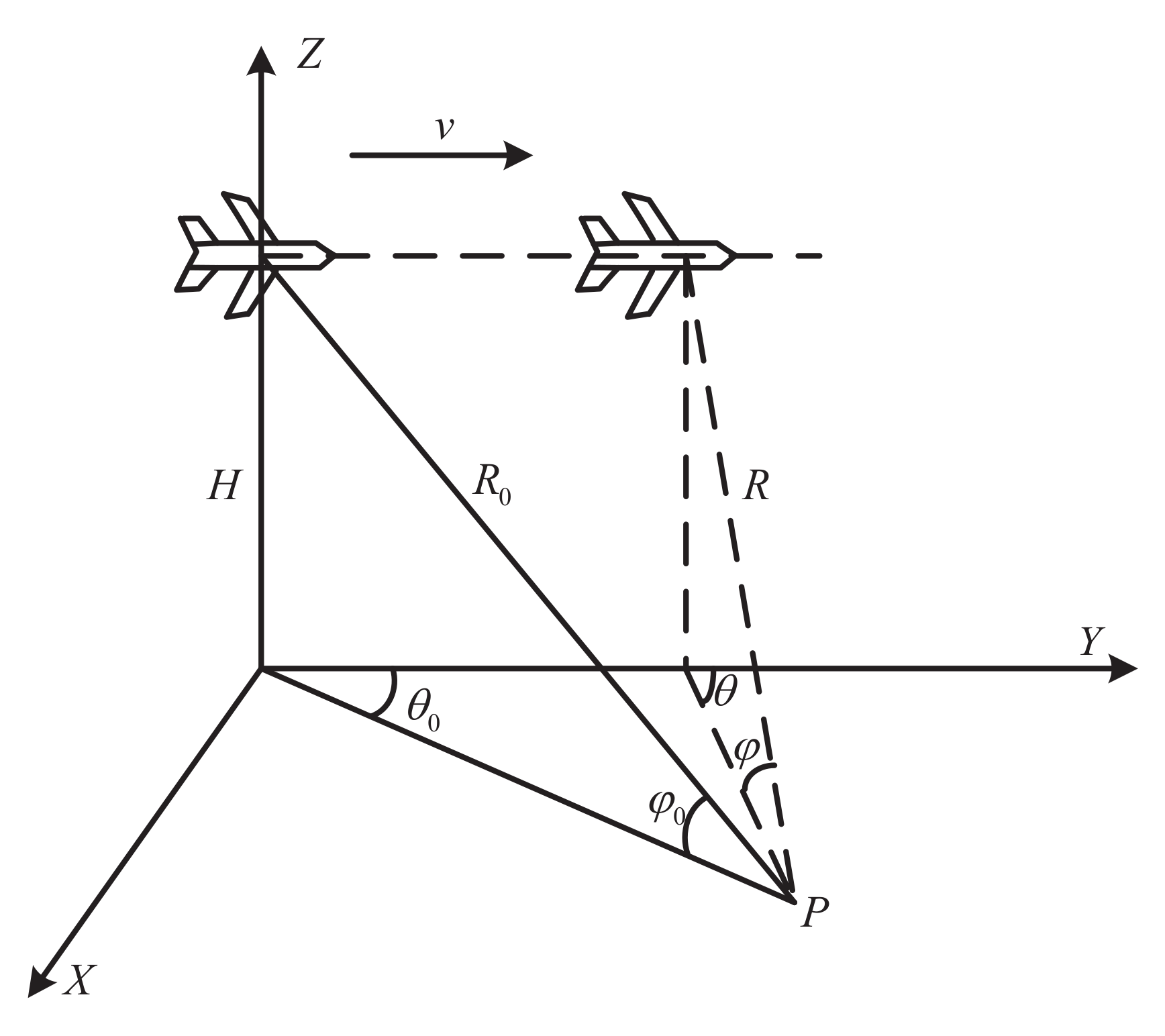
2.1. Azimuth Signal Model for Scanning Radar Forward-Looking Imaging

In this section, we analyze the azimuth echo signal convolution model of the forward-looking imaging. Figure 1 shows the geometric model of scanning radar. With a velocity of $\mathit{v}$ and a height of $\mathit{H}$, the aircraft travels in the Y-direction. $R_0$ is the initial slant range between the radar and the target P. ${\theta }_0$ is the initial azimuth angle. ${\phi }_0$ is the initial pitching angle. As the aircraft travels, the slant range changes into R, the pitching angle changes into $\phi$, and the azimuth angle changes into $\theta$ with a time interval t. The slant range history $R\left(t\right)$ satisfies

$$\begin{array}{cc}\hfill R\left(t\right)& =\sqrt{R_0^2+{\left(vt\right)}^2-2R_{0}vtcos{\theta }_{0}cos{\phi }_0}\hfill \\ \hfill & \approx R_0-vtcos{\theta }_{0}cos{\phi }_0.\hfill \end{array}$$

(3)

In the forward-looking region, the azimuth angle is normally smaller than ${10}^{\circ }$, and $cos{\theta }_0\approx 1$. So the approximate slant range history is written as

$$R\left(t\right)\approx R_0-vtcos{\phi }_0=R_0-vcos{\phi }_0\frac{\theta -{\theta }_0}{\omega }$$

(4)

where $\omega$ is the beam scanning speed.

The radar transmits LFM signal:

$$\begin{array}{cc}\hfill & s\left(\tau \right)=rect\left(\frac{\tau }{T_p}\right)exp\left(j2\pi f_c\tau \right)exp\left(j\pi \mu {\tau }^2\right)\hfill \end{array}$$

(5)

where $\tau$ is the fast time in range direction. $f_c$ denotes the carrier frequency of the transmitted signal. $T_p$ denotes the signal duration. $\mu$ denotes the chirp rate. $\mathrm{rect}\left(·\right)$ is written as

$$\mathrm{rect}\left(\frac{\tau }{T_p}\right)=\left\{\begin{array}{c}1,\\ 0,\end{array}\right.\begin{array}{c}\left|\tau \right|\le T_p/2\\ \left|\tau \right|>T_P/2\end{array}.$$

(6)

The received signal of the target P is denoted as follows:

$$\begin{array}{cc}\hfill & s_r\left(\tau ,t\right)\hfill \\ \hfill & ={\sigma }_{P}h\left(t-t_0\right)rect\left(\frac{\tau -2R\left(t\right)/c}{T_p}\right)\hfill \\ \hfill & ·exp\left(j2\pi f_c\left(\tau -\frac{2R\left(t\right)}{c}\right)\right)exp\left(j\pi \mu {\left(\tau -\frac{2R\left(t\right)}{c}\right)}^2\right)\hfill \end{array}$$

(7)

where $h\left(·\right)$ is the antenna pattern function, and ${\sigma }_P$ is the target scattering coefficient. $t_0$ is the time when the beam center scans P.

To achieve a high resolution in range direction, the pulse compression technique is implemented. The received signal is transformed to frequency domain in range direction

$$\begin{array}{cc}\hfill & s_r\left(f,t\right)\hfill \\ \hfill & ={\sigma }_{P}h\left(t-t_0\right)rect\left(\frac{f}{B_r}\right)exp\left(-j\frac{4\pi \left(f_c+f\right)}{c}R\left(t\right)\right)exp\left(-j\pi \frac{f^2}{\mu }\right)\hfill \end{array}$$

(8)

where f is the frequency in the range direction. Then, construct the frequency-domain filter

$$H\left(f\right)=rect\left(\frac{f}{B_r}\right)exp\left(j\pi \frac{f^2}{\mu }\right).$$

(9)

Multiply Equation (8) times Equation (9),

$$\begin{array}{cc}\hfill S_{rout}\left(f,t\right)& =S_r\left(f,t\right)H\left(f\right)\hfill \\ \hfill & ={\sigma }_{P}h\left(t-t_0\right)rect\left(\frac{f}{B_r}\right)exp\left(-j\frac{4\pi \left(f_c+f\right)}{c}R\left(t\right)\right).\hfill \end{array}$$

(10)

Transform the filtered signal to time domain in range direction, and get the received signal after pulse compression

$$s_{rout}\left(\tau ,t\right) = {\sigma }_{P}h\left(t-t_0\right)\sin \mathrm{c}\left[B_r\left(\tau -\frac{2R_0}{c}\right)\right]exp\left(-j\frac{4\pi }{\lambda }R\left(t\right)\right)$$

(11)

where $exp\left(-j4\pi R\left(t\right)/\lambda \right)$ is the Doppler shift which is approximately constant and can be ignored. Then, the received signal is transformed from the time domain $\left(\tau ,t\right)$ to range-angle domain as follows:

$$s_{rout}\left(R,\theta \right) = {\sigma }_{P}h\left(\theta -{\theta }_0\right)\sin \mathrm{c}\left[2B_r\left(\frac{R-R_0}{c}\right)\right]$$

(12)

Subsequently, the azimuth echo signal can be seen as a convolution form between the antenna pattern and the target scattering coefficient

$$s_{rout}\left(R,\theta \right)=\sigma \left(R,\theta \right)\otimes h\left(\theta \right)$$

(13)

where ⊗ denotes convolution operator.

Considering the interference, we have

$$s_{rout}\left(R,\theta \right)=\sigma \left(R,\theta \right)\otimes h\left(\theta \right)+w\left(\theta \right).$$

(14)

In Equation (14), the convolution can be written as a matrix multiplied by vector,

$$\mathbf{s}=\mathbf{H}\mathbf{x}+\mathbf{w}$$

(15)

where $\mathbf{s}$ represents the discrete azimuth echo signal vector defined as $\mathbf{s}={\left[s_1,\cdots ,s_M\right]}^T$. M is the length of the azimuth echo signal vector. ${(·)}^T$ denotes the transpose operation. $\mathbf{x}$ is the target vector defined as $\mathbf{x}={\left[x_1,\cdots ,x_K\right]}^T$. K is the length of scanning points in azimuth direction. $\mathbf{w}={\left[w_1,\cdots ,w_M\right]}^T$ denotes the interference of the clutter and noise. $\mathbf{H}$ denotes the convolution matrix

$$\mathbf{H}={\left[\begin{array}{cccc}{h}_1& & & \\ h_2& h_1& & \\ ⋮& h_2& \ddots & \\ h_L& ⋮& \ddots & h_1\\ & h_L& ⋮& h_2\\ & & \ddots & ⋮\\ & & & h_L\end{array}\right]}_{M\times K}.$$

(16)

where ${\left[h_1,\cdots ,h_L\right]}^T$ is antenna pattern vector. L is the length of the antenna pattern.

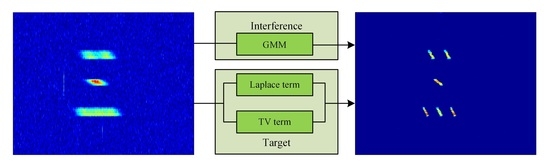
2.2. Bayesian Model for Sea-Surface Target

In this section, we propose a multi-prior Bayesian method to overcome the low resolution of the sea-surface target in azimuth direction and preserve the contour information. Firstly, we present the statistical distributions of the interference and target, respectively, and establish the Bayesian model. Secondly, we estimate the parameters by the MAP-EM method.

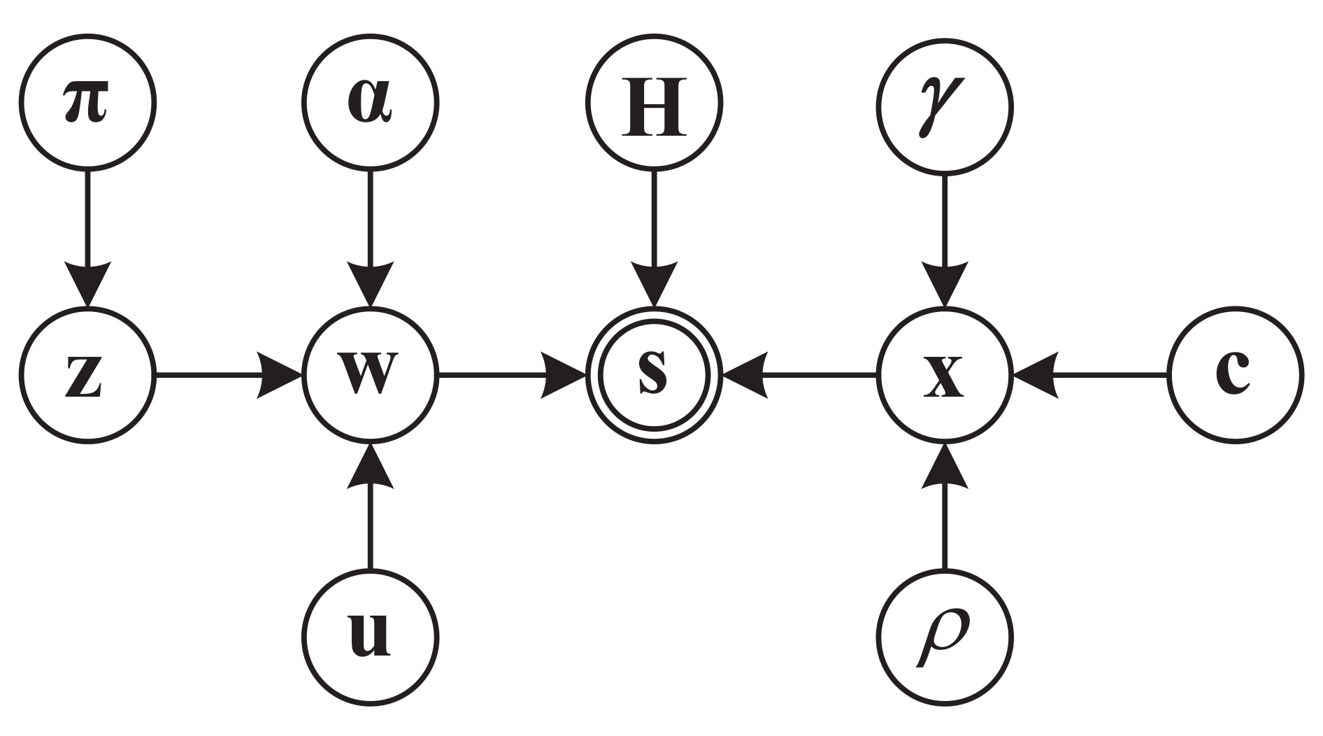
2.2.1. Bayesian Model

When the imaging target is the sea-surface target, the scene may be a sea-surface scene or a seacoast scene. The interference of the clutter and noise is challenging to model using a naive prior information. In [46,47,48], the authors propose that any continuous density could be approximated by a sufficient number of Gaussians. Inspired by this idea, we utilize the GMM to describe the interference.

$$p\left(w_m\right)=\sum _{j=1}^J{\pi }_{j}N\left(u_j,{\alpha }_j^{-1}\right)$$

(17)

where J is the number of Gaussians, ${\pi }_j$ is the weighted coefficient of the jth Gaussian, and ${\sum }_{j=1}^J{\pi }_j=1$, ${\pi }_j\ge 0$. $N\left(·\right)$ is Gaussian distribution function. $u_j$ is the mean value of the jth Gaussian. ${\alpha }_j$ is the inverse variance of the jth Gaussian.

In [48], the authors introduce Gamma-Gaussian prior to characterizing the sparsity of the target, and the result is effective. However, for some sea-surface targets, the targets are not only sparse, but also have contour information. To retain the contour information of the sea-surface targets, the TV prior is usually utilized [39], and the TV prior is written as

$$p\left(\mathbf{x}|\rho \right)={\left(\frac{\rho }{2}\right)}^K\exp \left(-\rho \mathrm{TV}\left(\mathbf{x}\right)\right)$$

(18)

where $\rho$ is the scaling parameter of the TV term. The high resolution of the range direction is realized by pulse compression technique in forward-looking imaging. Therefore, we only consider the azimuth dimension. The TV function is given by

$$\mathrm{TV}\left(\mathbf{x}\right)={∥\tilde{\mathbf{x}}∥}_1$$

(19)

where $\tilde{\mathbf{x}}=\mathbf{A}\mathbf{x}$. $\mathbf{A}$ is a discrete derivative operator

$$\mathbf{A}={\left[\begin{array}{ccccc}1& & & & \\ -1& 1& & & \\ & \ddots & \ddots & & \\ & & -1& 1& \\ & & & -1& 1\end{array}\right]}_{K\times K}.$$

(20)

At the same time, the sparse information of the target is modeled by the Laplace prior distribution.

$$p\left(\mathbf{x}\right|\gamma )={\left(\frac{\gamma }{2}\right)}^K\exp \left(-\gamma {∥\mathbf{x}∥}_1\right)$$

(21)

where $\gamma$ is the scaling parameter of the Laplace term.

We fuse the sparsity and contour information of the target, and the multi-prior distribution is defined as

$$p\left(\mathbf{x}\right|\mathbf{\gamma },\rho )=\prod _{k=1}^K\frac{{\gamma }_k\rho }{2}\exp \left(-c_1{\gamma }_k\left|x_k\right|-c_2\rho \left|{\tilde{x}}_k\right|\right)$$

(22)

where $c_1$ and $c_2$ are the weighted parameters to balance the Laplace term and the TV term. At the same time, to improve the flexibility of the sparse target scattering coefficient, we assume the Laplace distribution with different ${\gamma }_k$.

Figure 2 displays the probabilistic graphical model of the multi-prior Bayesian method, where $\mathbf{c}={[c_1,c_2]}^T$.

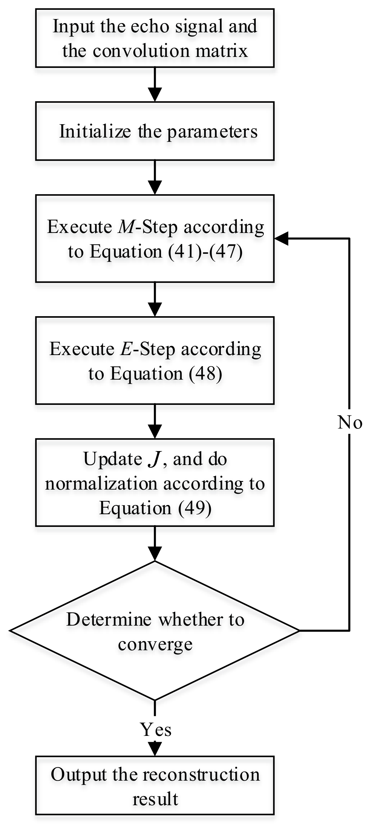
2.2.2. MAP-EM Estimation

To achieve high azimuth resolution, we need to do MAP estimation of the target scattering coefficient $\mathbf{x}$

$${\widehat{\mathbf{x}}}_{\mathrm{MAP}}=\underset{\mathbf{x}}{argmax}p\left(\mathbf{x}|\mathbf{s},\mathbf{\alpha },\mathbf{u},\mathbf{\pi }\right)$$

(23)

where $p\left(\mathbf{x}|\mathbf{s},\mathbf{\alpha },\mathbf{u},\mathbf{\pi }\right)$ is the posterior probability. The posterior $p\left(\mathbf{x}|\mathbf{s},\mathbf{\alpha },\mathbf{u},\mathbf{\pi }\right)$ is given by

$$p\left(\mathbf{x}|\mathbf{s},\mathbf{\alpha },\mathbf{u},\mathbf{\pi }\right)=\frac{p\left(\mathbf{s},\mathbf{x},\mathbf{\alpha },\mathbf{u},\mathbf{\pi }\right)}{\int p\left(\mathbf{s},\mathbf{x},\mathbf{\alpha },\mathbf{u},\mathbf{\pi }\right)d\mathbf{x}}.$$

(24)

However, the posterior $p\left(\mathbf{x}|\mathbf{s},\mathbf{\alpha },\mathbf{u},\mathbf{\pi }\right)$ is intractable, since $\int p\left(\mathbf{s},\mathbf{x},\mathbf{\alpha },\mathbf{u},\mathbf{\pi }\right)d\mathbf{x}$ cannot be calculated easily. Therefore, we use the joint probability $p\left(\mathbf{s},\mathbf{x},\mathbf{\alpha },\mathbf{u},\mathbf{\pi }\right)$ to perform the estimation. Then, the target scattering coefficient $\mathbf{x}$ is estimated by solving

$$\begin{array}{cc}\hfill {\widehat{\mathbf{x}}}_{\mathrm{MAP}}& =\underset{\mathbf{x}}{argmax}p\left(\mathbf{s},\mathbf{x},\mathbf{\alpha },\mathbf{u},\mathbf{\pi }\right)\hfill \\ \hfill & =\underset{\mathbf{x}}{argmax}lnp\left(\mathbf{s},\mathbf{x},\mathbf{\alpha },\mathbf{u},\mathbf{\pi }\right).\hfill \end{array}$$

(25)

The joint distribution satisfies

$$\begin{array}{cc}\hfill & p\left(\mathbf{s},\mathbf{x},\mathbf{\pi },\mathbf{\alpha },\mathbf{u}\right)\hfill \\ \hfill & =p\left(\mathbf{s}|\mathbf{x},\mathbf{\pi },\mathbf{\alpha },\mathbf{u}\right)p\left(\mathbf{x}|\mathbf{\gamma },\rho \right)\hfill \\ \hfill & =\prod _{m=1}^M\left(\sum _{j=1}^J{\pi }_{j}N\left(s_m|{\mathbf{H}}_m\mathbf{x}+u_j,{\alpha }_j^{-1}\right)\right)p\left(\mathbf{x}|\mathbf{\gamma },\rho \right).\hfill \end{array}$$

(26)

The logarithm likelihood function is written as

$$\begin{array}{cc}\hfill & lnp(\mathbf{s},\mathbf{x},\mathbf{\pi },\mathbf{\alpha },\mathbf{u})\hfill \\ \hfill & =\sum _{m=1}^M\ln \left(\sum _{j=1}^J{\pi }_{j}N\left(s_m|{\mathbf{H}}_m\mathbf{x}+u_j,{\alpha }_j^{-1}\right)\right)\hfill \\ \hfill & -c_1\sum _{k=1}^K{\gamma }_k\left|x_k\right|-c_2\rho \sum _{k=1}^K\left|{\tilde{x}}_k\right|+\mathrm{const}.\hfill \end{array}$$

(27)

Since the likelihood function contains $\ln \left(\sum \left(·\right)\right)$, the calculation is complex. To simplify Equation (27), we introduce a latent variable $\mathbf{z}={\left[z_1,\cdots ,z_M\right]}^T$, and $z_m$ satisfies

$$p(z_m=j)={\pi }_j$$

(28)

where $z_m$ denotes the sub-interference class label of the mth interference $w_m$. Because $z_m$ is determined from 1 to J, Equation (28) can be rewritten as

$$p\left(z_m\right)={\pi }_j^{1\left(z_m=j\right)}$$

(29)

where $1\left(z_m=j\right)$ is equal to 1 if $z_m=j$; or 0, otherwise.

Similarly, $p\left(w_m\right|z_m,\mathbf{u},\mathbf{\alpha })$ is written as

$$p\left(w_m|z_m,\mathbf{u},\mathbf{\alpha }\right)=\prod _{j=1}^J{\left(N\left(w_m|u_j,{\alpha }_j^{-1}\right)\right)}^{1\left(z_m=j\right)}.$$

(30)

Figure 3 displays the modified probabilistic graphical model. The joint distribution $p(\mathbf{s},\mathbf{z},\mathbf{x},\mathbf{\alpha },\mathbf{u})$ can be rewritten as

$$\begin{array}{cc}\hfill & p\left(\mathbf{s},\mathbf{z},\mathbf{x},\mathbf{\pi },\mathbf{\alpha },\mathbf{u}\right)\hfill \\ \hfill & =\left(\prod _{m=1}^M\prod _{j=1}^J{\left({\pi }_{j}N\left(s_m|{\mathbf{H}}_m\mathbf{x}+u_j,{\alpha }_j^{-1}\right)\right)}^{1\left({\mathrm{z}}_m=j\right)}\right)p\left(\mathbf{x}|\mathbf{\gamma },\rho \right).\hfill \end{array}$$

(31)

The logarithm likelihood function can be rewritten as

$$\begin{array}{cc}\hfill & lnp(\mathbf{s},\mathbf{z},\mathbf{x},\mathbf{\pi },\mathbf{\alpha },\mathbf{u})\hfill \\ \hfill & =\sum _{m=1}^M\sum _{j=1}^{J}1\left({\mathrm{z}}_m=j\right)\left(ln{\pi }_j+\frac{1}{2}ln{\alpha }_j-\frac{1}{2}{\alpha }_j{\left(s_m-{\mathbf{H}}_m\mathbf{x}-u_j\right)}^2\right)\hfill \\ \hfill & -c_1\sum _{k=1}^K{\gamma }_k\left|x_k\right|-c_2\rho \sum _{k=1}^K\left|{\tilde{x}}_k\right|+\mathrm{const}.\hfill \end{array}$$

(32)

From Equation (32), we can see that it is challenging to calculate $\mathbf{x}$ directly. In this section, we estimate the target scattering coefficients using MAP-EM approach [49].

The MAP-EM method is an iterative algorithm consisting of E-step and M-step. The latent variable $\mathbf{z}$ can be estimated in E-step, and the parameter $\{\mathbf{x},\mathbf{\pi },\mathbf{\alpha },\mathbf{u}\}$ is estimated in M-step.

The posterior distribution of $\mathbf{z}$ satisfies

$$p\left(\mathbf{z}|\mathbf{s},\mathbf{x},\mathbf{\pi },\mathbf{\alpha },\mathbf{u}\right)=\prod _{m=1}^{M}p\left(z_m|s_m,\mathbf{x},\mathbf{\pi },\mathbf{\alpha },\mathbf{u}\right)$$

(33)

where

$$\begin{array}{cc}\hfill & p\left(z_m|s_m,\mathbf{x},\mathbf{\pi },\mathbf{\alpha },\mathbf{u}\right)\hfill \\ \hfill & =\frac{p\left(s_m|z_m,\mathbf{x},\mathbf{\alpha },\mathbf{u}\right)p\left(z_m|\mathbf{\pi }\right)}{{\sum }_{j=1}^{J}p\left(s_m|z_m=j,\mathbf{x},\mathbf{\alpha },\mathbf{u}\right)p\left(z_m=j|\pi \right)}\hfill \\ \hfill & =\frac{{\pi }_{z_m}N\left(s_m|{\mathbf{H}}_m\mathbf{x}+u_{z_m},{\alpha }_{z_m}^{-1}\right)}{{\sum }_{j=1}^J{\pi }_{j}N\left(s_m|{\mathbf{H}}_m\mathbf{x}+u_j,{\alpha }_j^{-1}\right)}.\hfill \end{array}$$

(34)

We define

$$\begin{array}{cc}\hfill {\varphi }_m\left(j\right)& =p\left(z_m=j|s_m,\mathbf{x},{\pi }_j,{\alpha }_j,u_j\right)\hfill \\ \hfill & =\frac{{\pi }_{j}N\left(s_m|{\mathbf{H}}_m\mathbf{x}+u_j,{\alpha }_j^{-1}\right)}{{\sum }_{j=1}^J{\pi }_{j}N\left(s_m|{\mathbf{H}}_m\mathbf{x}+u_j,{\alpha }_j^{-1}\right)}.\hfill \end{array}$$

(35)

where ${\varphi }_m\left(j\right)$ is the posterior probability of the jth Gaussian in the mth observation, ${\sum }_{j=1}^J{\varphi }_m\left(j\right)=1$.

By maximizing the lower bound, the model parameter $\{\mathbf{x},\mathbf{\pi },\mathbf{\alpha },\mathbf{u}\}$ can be obtained, and the lower bound is given as

$$\begin{array}{cc}\hfill & L\left(\mathbf{x},\mathbf{\pi },\mathbf{\alpha },\mathbf{u}\right)\hfill \\ \hfill & =E_{\mathbf{z}|\mathbf{s},\mathbf{x},\mathbf{\pi },\mathbf{\alpha },\mathbf{u}}\left[\ln p(\mathbf{s},\mathbf{z},\mathbf{x},\mathbf{\pi },\mathbf{\alpha },\mathbf{u})\right]\hfill \\ \hfill & =\sum _{m=1}^M\sum _{j=1}^J{\psi }_m\left(j\right)\left(ln{\pi }_j+\frac{1}{2}ln{\alpha }_j-\frac{1}{2}{\alpha }_j{\left(s_m-{\mathbf{H}}_m\mathbf{x}-u_j\right)}^2\right)\hfill \\ \hfill & -c_1{∥\mathsf{\Gamma }\mathbf{x}∥}_1-c_2\rho {∥\tilde{\mathbf{x}}∥}_1+\mathrm{const}\hfill \end{array}$$

(36)

where $\mathsf{\Gamma }=\mathrm{diag}\left\{{\gamma }_1,\dots ,{\gamma }_K\right\}$.

Then, we obtain the model parameter $\{\mathbf{x},\mathbf{\pi },\mathbf{\alpha },\mathbf{u}\}$ by solving the gradient of the lower bound ${\nabla }_{\mathbf{x},\mathbf{\pi },\mathbf{\alpha },\mathbf{u}}L\left(\mathbf{x},\mathbf{\pi },\mathbf{\alpha },\mathbf{u}\right)=0$. Since $L_1$ norm is non-differentiable, we introduce the approximate approach,

$${∥\mathsf{\Gamma }\mathbf{x}∥}_1\approx \sum _{k=1}^K{\gamma }_k\sqrt{{\left|x_k\right|}^2+\delta }$$

(37)

$${∥\tilde{\mathbf{x}}∥}_1\approx \sum _{k=1}^K\sqrt{{\left|{\tilde{x}}_k\right|}^2+\delta }$$

(38)

where $\delta$ is a small non-negative constant.

The lower bound $L\left(\mathbf{x},\mathbf{\pi },\mathbf{\alpha },\mathbf{u}\right)$ is rewritten as

$$\begin{array}{cc}\hfill & L\left(\mathbf{x},\mathbf{\pi },\mathbf{\alpha },\mathbf{u}\right)\hfill \\ \hfill & =\sum _{m=1}^M\sum _{j=1}^J{\psi }_m\left(j\right)\left(ln{\pi }_j+\frac{1}{2}ln{\alpha }_j-\frac{1}{2}{\alpha }_j{\left(s_m-{\mathbf{H}}_m\mathbf{x}-u_j\right)}^2\right)\hfill \\ \hfill & -c_1\sum _{k=1}^K{\gamma }_k\sqrt{{\left|x_k\right|}^2+\delta }-c_2\rho \sum _{k=1}^K\sqrt{{\left|{\tilde{x}}_k\right|}^2+\delta }+\mathrm{const}.\hfill \end{array}$$

(39)

The solutions of ${\nabla }_{\mathbf{x},\mathbf{\pi },\mathbf{\alpha },\mathbf{u}}L\left(\mathbf{x},\mathbf{\pi },\mathbf{\alpha },\mathbf{u}\right)=0$ are

$$d_j=\sum _{m=1}^M{\psi }_m\left(j\right)$$

(40)

$${\pi }_j=\frac{d_j}{M}$$

(41)

$$\begin{array}{cc}\hfill \mathbf{x} & = {\left(\sum _{m=1}^M\left(\sum _{j=1}^J{\psi }_m\left(j\right){\alpha }_j\right){\mathbf{H}}_m^T{\mathbf{H}}_m+c_1\mathbf{U}\left(\mathbf{x}\right)+c_2\mathbf{W}\left(\tilde{\mathbf{x}}\right)\right)}^{-1}\hfill \\ \hfill & ·\sum _{m=1}^M\left(\sum _{j=1}^J{\psi }_m\left(j\right){\alpha }_j\left(s_m-u_j\right){\mathbf{H}}_m^T\right)\hfill \end{array}$$

(42)

where

$$\begin{array}{cc}\hfill & \mathbf{U}\left(\mathbf{x}\right)=\mathrm{diag}\left\{{\gamma }_1{\left(|x_1{|}^2+\delta \right)}^{-\frac{1}{2}},\dots ,{\gamma }_K{\left(|x_K{|}^2+\delta \right)}^{-\frac{1}{2}}\right\}\hfill \end{array}$$

(43)

$$\begin{array}{cc}\hfill & \mathbf{W}\left(\tilde{\mathbf{x}}\right)=\rho {\mathbf{A}}^T\mathrm{diag}\left\{{\left({\left|{\tilde{x}}_1\right|}^2+\delta \right)}^{-\frac{1}{2}},\dots ,{\left({\left|{\tilde{x}}_K\right|}^2+\delta \right)}^{-\frac{1}{2}}\right\}\mathbf{A}.\hfill \end{array}$$

(44)

For easy reference, we summarize the details of the proposed method.

Step 1: Initialize ${\psi }_m^{\left(1\right)}\left(j\right)$, ${\mathbf{\gamma }}^{\left(1\right)}$, ${\rho }^{\left(1\right)}$, ${\mathbf{u}}^{\left(1\right)}$, and ${\mathbf{\alpha }}^{\left(1\right)}$ randomly, and set $J^{\left(1\right)}$ with a large number, $x_k^{\left(1\right)}=\frac{{\mathbf{H}}_k^T\mathbf{s}}{{\mathbf{H}}_k^T{\mathbf{H}}_k}.$

Step 2:

M-step:

$$d_j^{\left(t+1\right)}=\sum _{m=1}^M{\psi }_m^{\left(t\right)}\left(j\right)$$

(45)

$${\pi }_j^{(t+1)}=\frac{d_j}{M}$$

(46)

$$\begin{array}{cc}\hfill & {\mathbf{x}}^{(t+1)}=\hfill \\ \hfill & {\left(\sum _{m=1}^M\left(\sum _{j=1}^J{\psi }_m^{\left(t\right)}\left(j\right){\alpha }_j^{\left(t\right)}\right){\mathbf{H}}_m^T{\mathbf{H}}_m+c_1\mathbf{U}\left({\mathbf{x}}^{\left(t\right)}\right)+c_2\mathbf{W}\left({\tilde{\mathbf{x}}}^{\left(t\right)}\right)\right)}^{-1}\hfill \\ \hfill & ·\sum _{m=1}^M\left(\sum _{j=1}^J{\psi }_m^{\left(t\right)}\left(j\right){\alpha }_j^{\left(t\right)}\left(s_m-u_j^{\left(t\right)}\right){\mathbf{H}}_m^T\right)\hfill \end{array}$$

(47)

$${\alpha }_j^{(t+1)}=\frac{d_j^{\left(t+1\right)}}{{\displaystyle \sum _{m=1}^M}{\psi }_m^{\left(t\right)}\left(j\right){\left(s_m-{\mathbf{H}}_m{\mathbf{x}}^{\left(t+1\right)}-u_j^{\left(t\right)}\right)}^2}$$

(48)

$$u_j^{\left(t+1\right)}=\frac{{\displaystyle \sum _{m=1}^M}{\psi }_m^{\left(t\right)}\left(j\right)\left(s_m-{\mathbf{H}}_m{\mathbf{x}}^{\left(t+1\right)}\right)}{d_j^{\left(t+1\right)}}$$

(49)

$${\gamma }_{{}_k}^{\left(t+1\right)}=\frac{1}{\left|x_k^{\left(t\right)}\right|+\delta }$$

(50)

$${\rho }^{\left(t+1\right)}=\frac{1}{{∥{\tilde{\mathbf{x}}}^{\left(t\right)}∥}_1+\delta }$$

(51)

E-step:

$${\psi }_m^{\left(t+1\right)}\left(j\right)=\frac{{\pi }_j^{\left(t+1\right)}N\left({\mathbf{H}}_m{\mathbf{x}}^{\left(t\right)}+u_j^{\left(t\right)},{\alpha }_j^{{\left(t\right)}^{-1}}\right)}{{\displaystyle \sum _{j=1}^J}{\pi }_j^{\left(t+1\right)}N\left({\mathbf{H}}_m{\mathbf{x}}^{\left(t\right)}+u_j^{\left(t\right)},{\alpha }_j^{{\left(t\right)}^{-1}}\right)}$$

(52)

Then, keep columns that correspond to the maximum probability of the mth input, update $J^{(t+1)}$, and do normalization ${\psi }_m^{(t+1)}\left(j\right)$

$${\psi }_m^{(t+1)}\left(j\right)={\psi }_m^{(t+1)}\left(j\right)/{\sum }_j{\psi }_m^{(t+1)}\left(j\right).$$

(53)

Step 3: Repeat Step 2 and calculate the difference value D until convergence.

$$D=\frac{L\left({\mathbf{x}}^{(t+1)},{\mathbf{\pi }}^{(t+1)},{\mathbf{\alpha }}^{(t+1)},{\mathbf{u}}^{(t+1)}\right)-L\left({\mathbf{x}}^{\left(t\right)},{\mathbf{\pi }}^{\left(t\right)},{\mathbf{\alpha }}^{\left(t\right)},{\mathbf{u}}^{\left(t\right)}\right)}{L\left({\mathbf{x}}^{\left(t\right)},{\mathbf{\pi }}^{\left(t\right)},{\mathbf{\alpha }}^{\left(t\right)},{\mathbf{u}}^{\left(t\right)}\right)}$$

(54)

In Step 1, we usually initialize J with a large number. To balance the Laplace term and the TV term, we need to manually pick appropriate weighted parameters, $c_1$ and $c_2$. To show the process more clearly, we give the flowchart of the multi-prior Bayesian method in Figure 4.

3. Experiment Result

To reflect the advantage of the multi-prior Bayesian method, we design multiple experiments in this section. We compare the imaging performance among IAA, SPICE, and Gaussian mixture model-Laplace hierarchical prior (GMM-LP) method [2,17,45]. In the experiments, the antenna pattern is Sinc-shaped and the main lobe is considered. The signal to clutter ratio (SCR) is given by

$$\mathrm{SCR}=10{log}_{10}\frac{P_s}{P_c}$$

(55)

where $P_s$ and $P_c$ are the mean power of the echo and the clutter, respectively.

The signal to noise ratio (SNR) is given by

$$\mathrm{SNR}=10{log}_{10}\frac{P_s}{P_n}$$

(56)

where $P_n$ is the mean power of the noise.

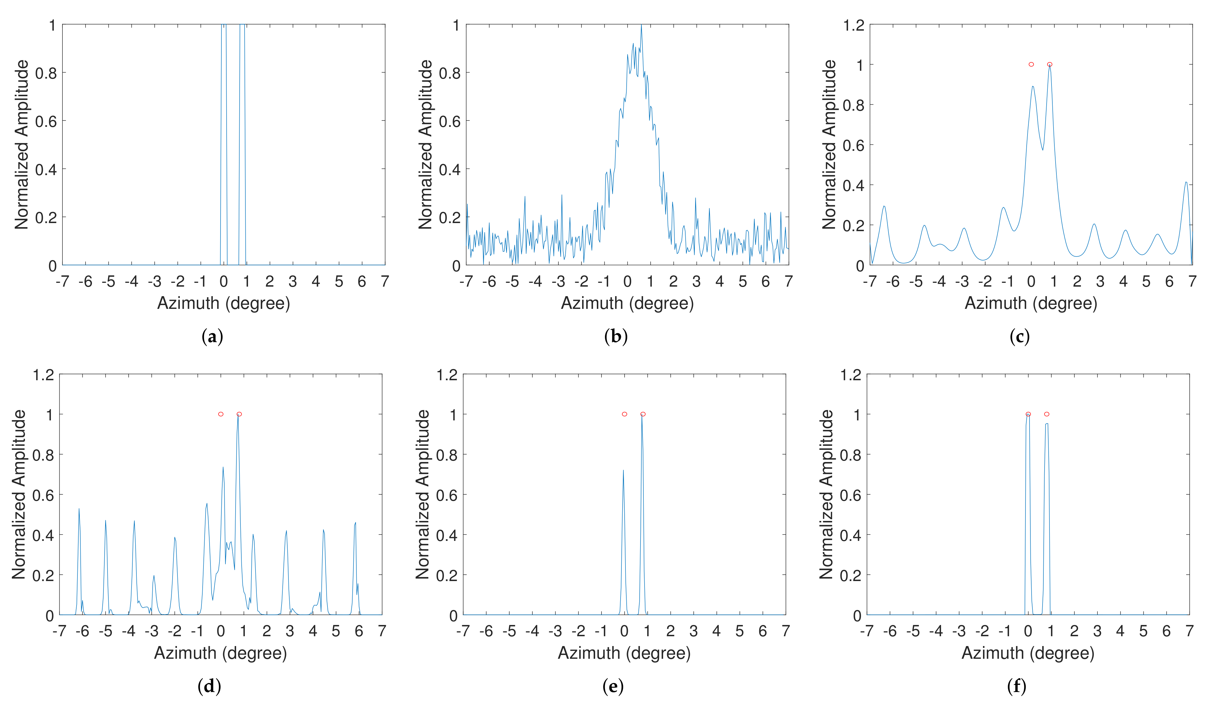
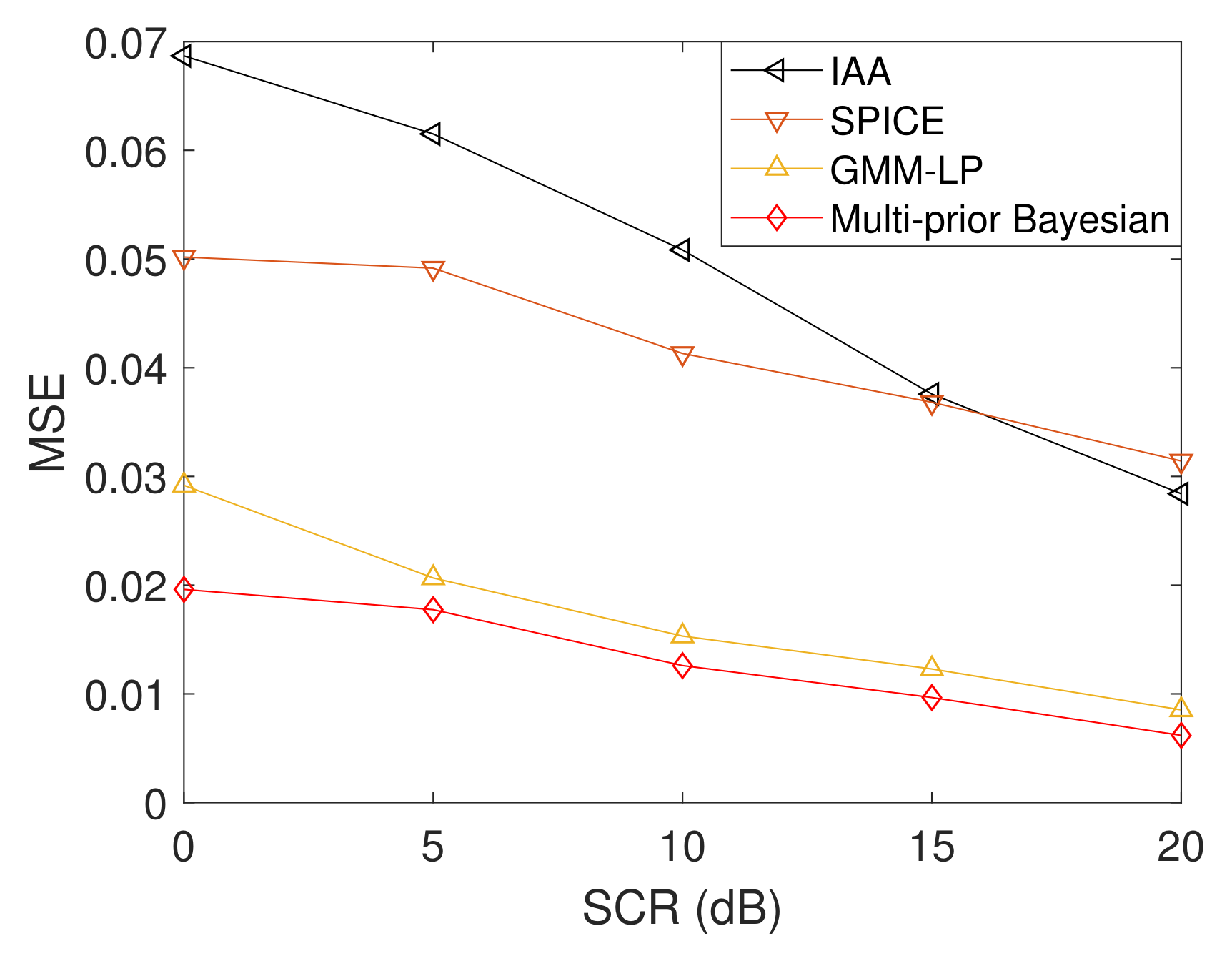
3.1. Point Simulation

The targets are assumed in the sea-surface scene. The performance of the multi-prior Bayesian method is verified by a point simulation. The sea clutter is modeled by Rayleigh distribution in this section.

Table 1. Point simulation parameters.

Parameter	Value
Bandwidth	60 MHz
Scanning speed	${50}^{\circ }/s$
Main Lobe Beamwidth	$3^{\circ }$
Pulse repetition frequency	1000 Hz

lists the simulation parameter. In the simulation, the scanning area in the azimuth direction covers from $-7^{\circ }\sim +7^{\circ }$. The antenna pattern is illustrated in Figure 5.

In the simulation, we assume the imaging region has two targets with the same amplitude. The positions of the targets are set at $0^{\circ }$ and $0.8^{\circ }$. The simulation results are shown in Figure 6. Figure 6a gives the ideal scene. Then, we add the Rayleigh clutter to the echo signal with SCR = 10 dB. Considering the system error, the white Gaussian noise is blended to the echo signal in the simulation with SNR = 20 dB. Figure 6b gives the echo signal result. Since the beam width is greater than the interval of adjacent targets, the adjacent targets are mixed. The processing results are shown in Figure 6c–f. The red circles are the ideal locations of the targets’ scattering. The processing result of the IAA method is displayed in Figure 6c. The two targets are separated, but the valley between the targets is high. The processing result of the SPICE method is displayed in Figure 6d. Affected by the clutter, many pseudo targets occur in the result of the SPICE method. Figure 6e displays the processing result of the GMM-LP method. It is obvious that the clutter is suppressed, and the targets are distinguished. Because the contour information is not considered in IAA, SPICE, and GMM-LP methods, the reconstruction results of the adjacent targets only have two sharp peaks. Figure 6f displays the processing result of the multi-prior Bayesian method. From the result, two targets are distinguished with low clutter. Meanwhile, the multi-prior Bayesian method also effectively retains the contour information of the targets.

To quantitatively reflect the superiority of the multi-prior Bayesian method, the mean square error (MSE) is employed, and the MSE is written as

$$\mathrm{MSE}=\frac{1}{N}\left(\frac{1}{K}{∥\widehat{\mathbf{x}}-\mathbf{x}∥}_2^2\right)$$

(57)

where $\widehat{\mathbf{x}}$ represents the estimation value, and $\mathbf{x}$ represents the ideal azimuth value. N denotes the number of Monte Carlo simulations. The SCR is set from 0 to 20 dB in experiments. For each SCR, we conduct 100 independent Monte Carol trials with SNR = 20 dB [50]. The MSE curves are shown in Figure 7. From the results, the multi-prior Bayesian method has a lower MSE curve. The MSE curves prove that the multi-prior Bayesian method performs better than other methods.

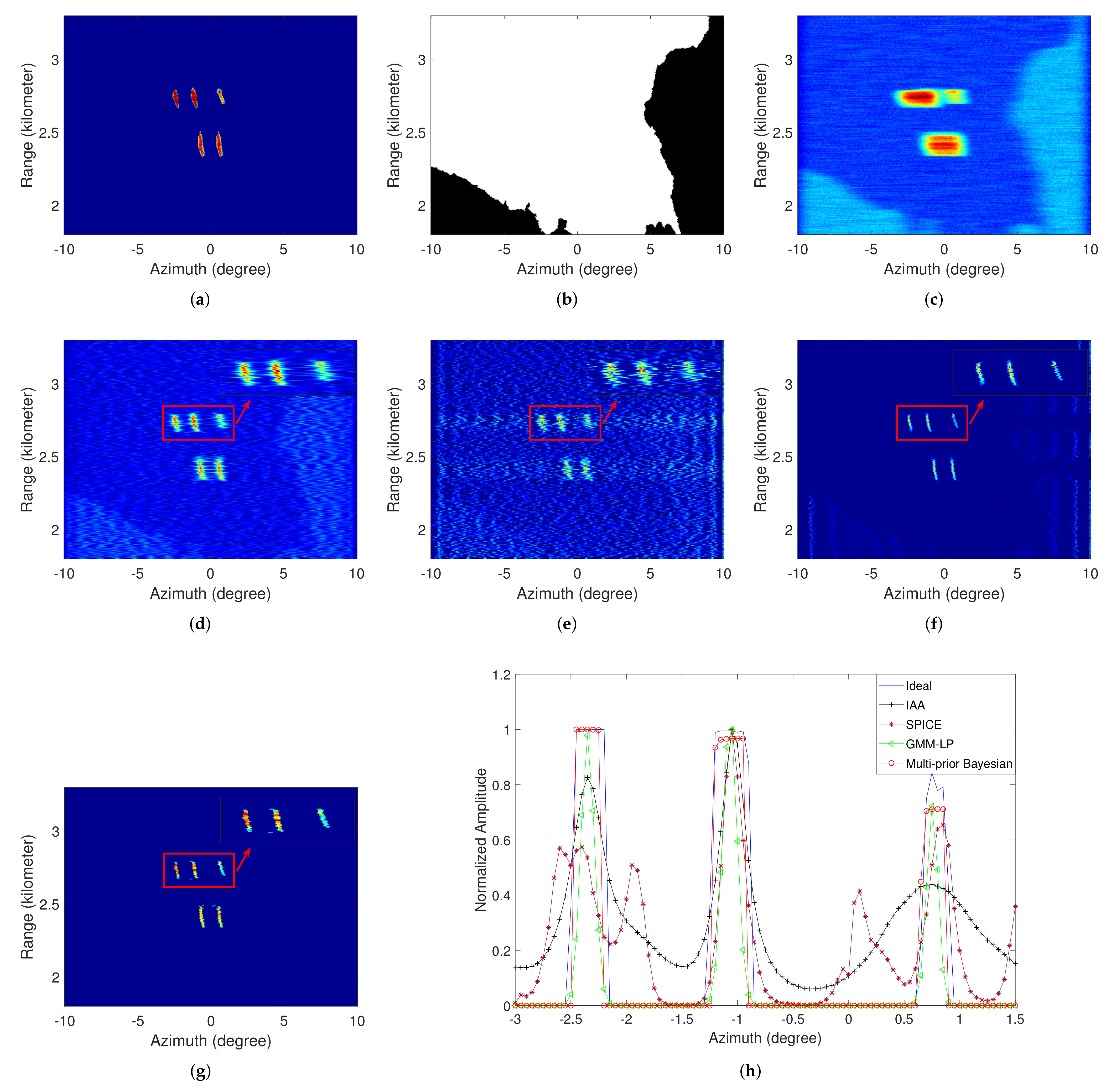
3.2. Area Simulation

To further understand the effectiveness of the multi-prior Bayesian method, the area simulation is considered in this section. In this case, the sea-surface targets are assumed in the seacoast. The ground clutter and the sea clutter are expressed by the Gaussian distribution and the Rayleigh distribution, respectively.

Table 2. Area simulation parameters.

Parameter	Value
Bandwidth	60 MHz
Scanning speed	${50}^{\circ }/s$
Scanning area	$-{10}^{\circ }\sim +{10}^{\circ }$
Main Lobe Beamwidth	$3^{\circ }$
Pulse repetition frequency	1000 Hz

lists the simulation parameters.

As shown in Figure 8a, we construct a synthetic scene with several adjacent targets in a different range cell. Figure 8b displays the clutter label. The black part is populated by the Rayleigh clutter, and the white part is populated by the Gaussian clutter. Then, we add the Gaussian noise to the echo signal with $\mathrm{SNR}=20 \mathrm{dB}$. The echo signal result is shown in Figure 8c with SCR = 5 dB. In the echo signal, the adjacent targets are mixed and cannot be distinguished. Figure 8d–g are the imaging results processed by IAA, SPICE, GMM-LP, and the multi-prior Bayesian method. The global resolution has been greatly enhanced in the results. From Figure 8d, we can see that the IAA method distinguishes all targets, but suffers from the clutter. In Figure 8e, the SPICE method can separate the targets the same as the IAA method, but the clutter is still not suppressed. As shown in Figure 8f, the GMM-LP method can reject the Rayleigh clutter and Gaussian clutter. Figure 8g is the processing result of the multi-prior Bayesian method. Figure 8g is more clarity, and the reconstruction targets are more obvious compared with other processing results. The results prove that the multi-prior Bayesian method can well resolve the targets with lower clutter.

To further view the processing results, we extract the profiles at range cell 2745 m, which are shown in Figure 8h. The targets are separated in the results of the IAA method. However, the sharpening effect of the right target is not well. Affected by the clutter, the left target has two peaks in the result of the SPICE method. The GMM-LP method can sharpen the beam, and the targets are separated with a low saddle. As we can see, the contour information is missing in the result of the GMM-LP method. Conversely, the multi-prior Bayesian method can distinguish all targets. Meanwhile, the contour information is well restored.

Table 3. MSE results at range cell 2745 m.

Methods	MSE ($\times {10}^{-2}$)
IAA	2.75
SPICE	3.91
GMM-LP	1.41
Multi-prior Bayesia	0.57

shows the MSE results of the different methods at range cell 2745 m. In Table 3, the multi-prior Bayesian method has a lower MSE value compared with other methods.

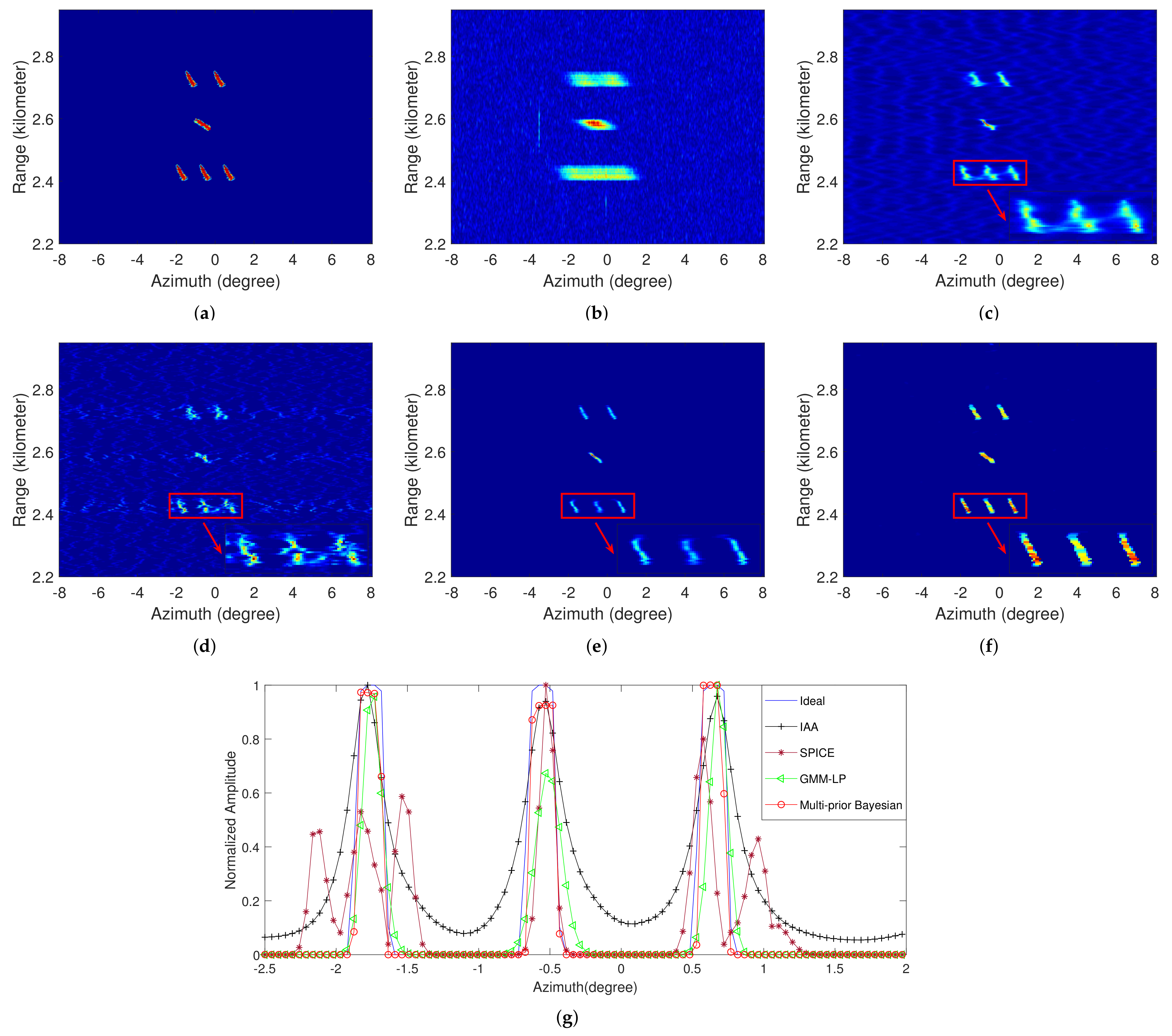
3.3. Semi-Real Data Experiment

The point and area simulations have proved the effectiveness of the multi-prior Bayesian method to overcome the low resolution of sea-surface targets in azimuth direction and preserve the contour information. In practical applications, the clutter is more complex compared with Rayleigh clutter or Gaussian clutter. We process the semi-real data in this part to verify the effectiveness of the multi-prior Bayesian method. The real data is X-band sea clutter and

Table 4. System parameters of semi-real data.

Parameter	Value
Bandwidth	25 MHz
Scanning speed	${144}^{\circ }$/s
Scanning area	$-8^{\circ }\sim +8^{\circ }$
Main Lobe Beamwidth	$2.7^{\circ }$
Pulse repetition frequency	3000 Hz

displays the parameters of the radar system [51]. The radar antenna of the real data is shown in Figure 9.

Figure 10a displays several targets in the ideal scene. It can be seen that the targets are sparse in the whole region, and have obvious contour information. The echo signal after pulse compression with SCR of $10\mathrm{dB}$ is shown in Figure 10b. The processing result of the IAA method is displayed in Figure 10c. The targets are distinguished and the azimuth resolution is improved in the result. However, the clutter still obviously exists. The contour information of the target is missed. Figure 10d displays the processing result of the SPICE method. The targets are picked out as shown in Figure 10d. However, the clutter is not restrained. The processing result of the GMM-LP method is given in Figure 10e. In Figure 10e, the azimuth resolution is improved effectively and the clutter is suppressed. The processing result of the multi-prior Bayesian method is given in Figure 10f. The targets are completely distinguished with a low clutter. At the same time, the contour information is restored well.

Figure 10g shows the profiles at range cell 2435 m. From the result, the IAA method can sharpen all the targets, but the high clutter still exists. In the result of the SPICE method, there are two or three peaks in a target. The GMM-LP method can reconstruct the sparse sea-surface targets, and effectively suppress the clutter. However, the contour information is missed. The multi-prior Bayesian method has a better reconstruction with low clutter. We then calculate the MSE results to quantitatively reflect the superiority of the multi-prior Bayesian method.

Table 5. MSE results at range cell 2435 m.

Methods	MSE ($\times {10}^{-2}$)
IAA	1.92
SPICE	2.59
GMM-LP	0.76
Multi-prior Bayesia	0.19

shows the results extracted from 2435 m range cell. From Table 5, the multi-prior Bayesian method has a better performance in the MSE results, which indicates that the multi-prior Bayesian method has greater clutter suppression and azimuth improvement capability than other approaches.

4. Discussion

In the forward-looking imaging of sea-surface target, the suitable model of the imaging environment plays an important role. However, most methods focus on the system noise and ignore the particular characteristics of the environment of the sea-surface target. Thus, only the Gaussian noise is considered. The multi-prior Bayesian method considers the characteristics of the environment of the sea-surface target, and proposes to use the GMM to model the clutter in the imaging scene. On the other hand, the sea-surface target also has many characteristics. For example, compared with the whole imaging scene, the target is sparse. In the autonomous landing on a ship, the counter information is important to influence the landing precision. The multi-prior Bayesian method fuses the sparsity and counter information to model the sea-surface target by introducing the Laplace prior and TV prior. Therefore, combining with the environment clutter and the target model, the multi-prior method can perform well in target recovery and clutter suppression. For the visual and quantitative results obtained in Section 3, the simulations and semi-real data processing results are presented to show the performance of the multi-prior Bayesian method. Compared with the traditional methods, the multi-prior method has a better performance both in the sea-surface scene and the seacoast scene.

In practical application, real time is crucial. The computation complexity of the multi-prior Bayesian method is mainly determined by the length of the echo signal M, the length of scanning points in azimuth direction K, the number of Gaussian distribution J. In E-step, computing the posterior probability ${\varphi }_m\left(j\right)$ needs $O\left(JM\right)$. In M-step, computing the parameters $\pi$, $\alpha$ and u requires $O\left(JM\right)$. Computing the parameter $\mathbf{x}$ requires computing the inverse matrix. The computational complexity to calculate the inverse matrix is $O\left(K^3\right)$. The overall computation complexity is concentrated in calculating the parameter $\mathbf{x}$. To improve the imaging speed, we will find an improved algorithm to reduce the computational complexity to calculate the inverse matrix.

In the multi-prior Bayesian method, the weighted parameter $\mathbf{c}$ is utilized to balance the Laplace term and the TV term. However, we need to manually pick the appropriate weighted parameter in the imaging procession. Future work will also research how to select the weighted parameter adaptively.

The high resolution in range direction is realized by the pulse compress technique. We only consider realizing the high resolution in the azimuth direction. Only one-dimensional prior information is exploited. However, two-dimensional prior information of the target can provide more structure information. In the future, two-dimensional prior information of the target is encouraged to study.

5. Conclusions

In this paper, to overcome low resolution in the azimuth direction and retain the contour information of the sea-surface target, we proposed a multi-prior Bayesian method to obtain forward-looking imaging. We used the GMM to model the interference considering the complexity of the interference in the forward-looking scene. In the imaging region, the sea-surface targets were not only sparse, but also had contour information. By fusing the Laplace prior distribution and the TV prior distribution, we proposed a multi-prior to describe the prior model of the sea-surface target. Since logarithm likelihood function existed in the accumulative-logarithmic operations, we introduced the latent variable to derive the logarithm likelihood function. The MAP-EM method was used to achieve the optimized solution. Finally, several experiments proved that the multi-prior Bayesian method obviously enhances the angular resolution and suppresses the clutter. At the same time, the contour information of the sea-surface target was restored well.

References

1. Chen, H.; Li, M.; Wang, Z.; Lu, Y.; Cao, R.; Zhang, P.; Zuo, L.; Wu, Y. Cross-Range Resolution Enhancement for DBS Imaging in a Scan Mode Using Aperture-Extrapolated Sparse Representation. IEEE Geosci. Remote Sens. Lett. 2017, 14, 1459–1463. [Google Scholar] [CrossRef]
2. Zhang, Y.; Zhang, Y.; Huang, Y.; Li, W.; Yang, J. Angular Superresolution for Scanning Radar With Improved Regularized Iterative Adaptive Approach. IEEE Geosci. Remote Sens. Lett. 2016, 13, 846–850. [Google Scholar] [CrossRef]
3. Li, W.; Niu, M.; Zhang, Y.; Huang, Y.; Yang, J. Forward-Looking Scanning Radar Superresolution Imaging Based on Second-Order Accelerated Iterative Shrinkage-Thresholding Algorithm. IEEE J. Sel. Topics Appl. Earth Observ. Remote Sens. 2020, 13, 620–631. [Google Scholar] [CrossRef]
4. Tan, K.; Li, W.; Pei, J.; Huang, Y.; Yang, J. An I/Q-Channel Modeling Maximum Likelihood Super-Resolution Imaging Method for Forward-Looking Scanning Radar. IEEE Geosci. Remote Sens. Lett. 2018, 15, 863–867. [Google Scholar] [CrossRef]
5. Wehner, D.R. High Resolution Radar; Norwood: Boston, MA, USA, 1987. [Google Scholar]
6. Li, W.; Zhang, W.; Zhang, Q.; Zhang, Y.; Huang, Y.; Yang, J. Simultaneous Super-Resolution and Target Detection of Forward-Looking Scanning Radar via Low-Rank and Sparsity Constrained Method. IEEE Trans. Geosci. Remote Sens. 2020, 58, 7085–7095. [Google Scholar] [CrossRef]
7. Skolnik, M.I. Radar Handbook, 3rd ed.; McGraw-Hill Education: New York, NY, USA, 2008. [Google Scholar]
8. Zhang, Q.; Zhang, Y.; Huang, Y.; Zhang, Y. Azimuth Superresolution of Forward-Looking Radar Imaging Which Relies on Linearized Bregman. IEEE J. Sel. Topics Appl. Earth Observ. Remote Sens. 2019, 12, 2032–2043. [Google Scholar] [CrossRef]
9. Quan, Y.; Zhang, R.; Li, Y.; Xu, R.; Zhu, S.; Xing, M. Microwave Correlation Forward-Looking Super-Resolution Imaging Based on Compressed Sensing. IEEE Trans. Geosci. Remote Sens. 2021, 59, 8326–8337. [Google Scholar] [CrossRef]
10. Dropkin, H.; Ly, C. Superresolution for Scanning Antenna. In Proceedings of the 1997 IEEE National Radar Conference, Syracuse, NY, USA, 13–15 May 1997; pp. 306–308. [Google Scholar]
11. Li, Y.; Liu, J.; Jiang, X.; Huang, X. Angular Superresol for Signal Model in Coherent Scanning Radars. IEEE Trans. Aerosp. Electron. Syst. 2019, 55, 3103–3116. [Google Scholar] [CrossRef]
12. Ly, C.; Dropkin, H.; Manitius, A.Z. Extension of the Music Algorithm to Millimeter-Wave (Mmw) Real-Beam Radar Scanning Antennas. In Proceedings of the Radar Sensor Technology and Data Visualization, Orlando, FL, USA, 1–5 April 2002; Volume 4744, pp. 96–107. [Google Scholar]
13. Zhang, Q.; Zhang, Y.; Zhang, Y.; Huang, Y.; Yang, J. A Sparse Denoising-Based Super-Resolution Method for Scanning Radar Imaging. Remote Sens. 2021, 13, 2768. [Google Scholar] [CrossRef]
14. Zhang, Q.; Zhang, Y.; Huang, Y.; Zhang, Y.; Pei, J.; Yi, Q.; Li, W.; Yang, J. TV-Sparse Super-Resolution Method for Radar Forward-Looking Imaging. IEEE Trans. Geosci. Remote Sens. 2020, 58, 6534–6549. [Google Scholar] [CrossRef]
15. Chen, H.; Li, Y.; Gao, W.; Zhang, W.; Sun, H.; Guo, L.; Yu, J. Bayesian Forward-Looking Superresolution Imaging Using Doppler Deconvolution in Expanded Beam Space for High-Speed Platform. IEEE Trans. Geosci. Remote Sens. 2021, in press. [Google Scholar] [CrossRef]
16. Zhang, Y.; Zhang, Y.; Li, W.; Huang, Y.; Yang, J. Super-Resolution Surface Mapping for Scanning Radar: Inverse Filtering Based on the Fast Iterative Adaptive Approach. IEEE Trans. Geosci. Remote Sens. 2017, 56, 127–144. [Google Scholar] [CrossRef]
17. Zhang, Y.; Jakobsson, A.; Zhang, Y.; Huang, Y.; Yang, J. Wideband Sparse Reconstruction for Scanning Radar. IEEE Trans. Geosci. Remote Sens. 2018, 56, 6055–6068. [Google Scholar] [CrossRef]
18. Fang, J.; Wang, F.; Shen, Y.; Li, H.; Blum, R.S. Super-Resolution Compressed Sensing for Line Spectral Estimation: An Iterative Reweighted Approach. IEEE Trans. Signal Process. 2016, 64, 4649–4662. [Google Scholar] [CrossRef]
19. Goldstein, T.; Osher, S. The split Bregman method for L1-regularized problems. SIAM J. Imag. Sci. 2009, 2, 323–343. [Google Scholar] [CrossRef]
20. Shea, J.D.; Van Veen, B.D.; Hagness, S.C. A TSVD Analysis of Microwave Inverse Scattering for Breast Imaging. IEEE Trans. Biomed. Eng. 2011, 59, 936–945. [Google Scholar] [CrossRef] [PubMed] [Green Version]
21. Gambardella, A.; Migliaccio, M. On the Superresolution of Microwave Scanning Radiometer Measurements. IEEE Geosci. Remote Sens. Lett. 2008, 5, 796–800. [Google Scholar] [CrossRef]
22. Yardibi, T.; Li, J.; Stoica, P.; Xue, M.; Baggeroer, A.B. Source Localization and Sensing: A Nonparametric Iterative Adaptive Approach Based on Weighted Least Squares. IEEE Trans. Aerosp. Electron. Syst. 2010, 46, 425–443. [Google Scholar] [CrossRef]
23. Stoica, P.; Babu, P.; Li, J. SPICE: A Sparse Covariance-Based Estimation Method for Array Processing. IEEE Trans. Signal Process. 2010, 59, 629–638. [Google Scholar] [CrossRef]
24. Zhang, Y.; Jakobsson, A.; Yang, J. Range-Recursive IAA for Scanning Radar Angular Super-Resolution. IEEE Geosci. Remote Sens. Lett. 2017, 14, 1675–1679. [Google Scholar] [CrossRef]
25. Ghaderpour, E. Multichannel antileakage least-squares spectral analysis for seismic data regularization beyond aliasing. Acta Geophys. 2019, 67, 1349–1363. [Google Scholar] [CrossRef]
26. Tipping, M.E. Sparse Bayesian Learning and the Relevance Vector Machine. J. Mach. Learn. Res. 2001, 1, 211–244. [Google Scholar]
27. Zhang, Y.; Huang, Y.; Zha, Y.; Yang, J. Superresolution Imaging for Forward-Looking Scanning Radar with Generalized Gaussian Constraint. Prog. Electromagn. Res. 2016, 46, 1–10. [Google Scholar] [CrossRef] [Green Version]
28. Bai, X.; Wang, G.; Liu, S.; Zhou, F. High-Resolution Radar Imaging in Low SNR Environments Based on Expectation Propagation. IEEE Trans. Geosci. Remote Sens. 2021, 59, 1275–1284. [Google Scholar] [CrossRef]
29. Zhou, F.; Bai, X. High-Resolution Sparse Subband Imaging Based on Bayesian Learning With Hierarchical Priors. IEEE Trans. Geosci. Remote Sens. 2018, 56, 4568–4580. [Google Scholar] [CrossRef]
30. Guan, J.; Yang, J.; Huang, Y.; Li, W. Maximum a Posteriori–Based Angular Superresolution for Scanning Radar Imaging. IEEE Trans. Aerosp. Electron. Syst. 2014, 50, 2389–2398. [Google Scholar] [CrossRef]
31. Chen, H.M.; Li, M.; Wang, Z.; Lu, Y.; Zhang, P.; Wu, Y. Sparse Super-Resolution Imaging for Airborne Single Channel Forward-Looking Radar in Expanded Beam Space via lp Regularisation. Electron. Lett. 2015, 51, 863–865. [Google Scholar] [CrossRef]
32. Tuo, X.; Zhang, Y.; Huang, Y.; Yang, J. Fast Sparse-TSVD Super-Resolution Method of Real Aperture Radar Forward-Looking Imaging. IEEE Trans. Geosci. Remote Sens. 2021, 59, 6609–6620. [Google Scholar] [CrossRef]
33. Zhang, Y.; Zhang, Q.; Zhang, Y.; Pei, J.; Huang, Y.; Yang, J. Fast Split Bregman Based Deconvolution Algorithm for Airborne Radar Imaging. Remote Sens. 2020, 12, 1747. [Google Scholar] [CrossRef]
34. Stoica, P.; Babu, P.; Li, J. New method of sparse parameter estimation in separable models and its use for spectral analysis of irregularly sampled data. IEEE Trans. Signal Process. 2011, 59, 35–47. [Google Scholar] [CrossRef]
35. Zhang, Y.; Zhang, Y.; Huang, Y.; Yang, J.; Jakobsson, A. Sparse source location for real aperture radar using generalized sparse covariance fitting. In Proceedings of the IEEE Radar Conference, Seattle, WA, USA, 8–12 May 2017; pp. 1069–1074. [Google Scholar]
36. Babacan, S.D.; Molina, R.; Katsaggelos, A.K. Bayesian Compressive Sensing Using Laplace Priors. IEEE Trans. Image Process. 2010, 19, 53–63. [Google Scholar] [CrossRef] [PubMed]
37. Chen, H.; Li, M.; Wang, Z.; Lu, Y.; Wang, S.; Zuo, L.; Zhang, P.; Wu, Y. Super-Resolution Doppler Beam Sharpening Imaging via Sparse Representation. IET Radar Sonar Navigat. 2016, 10, 442–448. [Google Scholar] [CrossRef]
38. Xu, G.; Xing, M.; Zhang, L.; Liu, Y.; Li, Y. Bayesian Inverse Synthetic Aperture Radar Imaging. IEEE Geosci. Remote Sens. Lett. 2011, 8, 1150–1154. [Google Scholar] [CrossRef]
39. Babacan, S.D.; Molina, R.; Katsaggelos, A.K. Parameter Estimation in TV Image Restoration Using Variational Distribution Approximation. IEEE Trans. Image Process. 2008, 17, 326–339. [Google Scholar] [CrossRef] [Green Version]
40. Zhang, Y.; Tuo, X.; Huang, Y.; Yang, J. A TV Forward-Looking Super-Resolution Imaging Method Based on TSVD Strategy for Scanning Radar. IEEE Trans. Geosci. Remote Sens. 2020, 58, 4517–4528. [Google Scholar] [CrossRef]
41. Huo, W.; Tuo, X.; Zhang, Y.; Zhang, Y.; Huang, Y. Balanced Tikhonov and Total Variation Deconvolution Approach for Radar Forward-Looking Super-Resolution Imaging. IEEE Geosci. Remote Sens. Lett. 2021, in press. [Google Scholar] [CrossRef]
42. Xu, S.; Zheng, J.; Pu, J.; Shui, P. Sea-Surface Floating Small Target Detection Based on Polarization Features. IEEE Geosci. Remote Sensing Lett. 2018, 15, 1505–1509. [Google Scholar] [CrossRef]
43. Liu, T.; Pang, B.; Ai, S.; Sun, X. Study on Visual Detection Algorithm of Sea Surface Targets Based on Improved YOLOv3. Sensors 2020, 20, 7263. [Google Scholar] [CrossRef]
44. Zhang, Y.; Zhang, Q.; Li, C.; Zhang, Y.; Huang, Y.; Yang, J. Sea-Surface Target Angular Superresolution in Forward-Looking Radar Imaging Based on Maximum a Posteriori Algorithm. IEEE J. Sel. Topics Appl. Earth Observ. Remote Sens. 2019, 12, 2822–2834. [Google Scholar] [CrossRef]
45. Li, W.; Li, M.; Zuo, L.; Sun, H.; Chen, H.; Lu, X. Azimuth Super-Resolution of Forward-Looking Imaging Based on Bayesian Learning in Complex Scene. Signal Process. 2021, 187, 108141. [Google Scholar] [CrossRef]
46. Pedersen, N.L.; Manchón, C.N.; Badiu, M.-A.; Shutin, D.; Fleury, B.H. Sparse Estimation Using Bayesian Hierarchical Prior Modeling for Real and Complex Linear Models. Signal Process. 2015, 115, 94–109. [Google Scholar] [CrossRef] [Green Version]
47. Meng, D.; De La Torre, F. Robust Matrix Factorization with Unknown Noise. In Proceedings of the IEEE International Conference on Computer Vision, Sydney, Australia, 2–8 December 2013; pp. 1337–1344. [Google Scholar]
48. Bai, X.; Zhang, Y.; Zhou, F. High-Resolution Radar Imaging in Complex Environments Based on Bayesian Learning with Mixture Models. IEEE Trans. Geosci. Remote Sens. 2019, 57, 972–984. [Google Scholar] [CrossRef]
49. Bishop, C.M. Pattern Recognition and Machine Learning; Springer: New York, NY, USA, 2006. [Google Scholar]
50. Robert, C.P.; Casella, G. Monte Carlo Statistical Methods; Springer: Berlin/Heidelberg, Germany, 2004. [Google Scholar]
51. Ningbo, L.; Yunlong, D.; Guoqing, W.; Hao, D.; Yong, H.; Jian, G.; Xiaolong, C.; You, H. Sea-detecting X-band radar and data acquisition program. J. Radars 2019, 8, 656–667. [Google Scholar]
Figure 1. Geometric model of the scanning radar.
Remotesensing 14 00026 g001
Figure 2. Probabilistic graphical model.
Remotesensing 14 00026 g002
Figure 3. Modified probabilistic graphical model with latent variable.
Remotesensing 14 00026 g003
Figure 4. The flowchart of the multi-prior Bayesian method.
Remotesensing 14 00026 g004
Figure 5. Antenna pattern.
Remotesensing 14 00026 g005
Figure 6. Point Simulation results. (a) Original scene. (b) Echo signal. (c) IAA method. (d) SPICE method. (e) GMM-LP method. (f) Multi-prior Bayesian method. (The red circles are the ideal locations of the targets’ scattering).
Remotesensing 14 00026 g006
Figure 7. MSE curves with Rayleigh distribution.
Remotesensing 14 00026 g007
Figure 8. Area simulation results. (a) Ideal scene. (b) Clutter label. (c) Echo signal. (d) IAA method. (e) SPICE method. (f) GMM-LP method. (g) Multi-prior Bayesian method. (h) Comparison at range cell 2745 m.
Remotesensing 14 00026 g008
Figure 9. Radar antenna of the real data.
Remotesensing 14 00026 g009
Figure 10. Results of semi-real data. (a) Ideal scene. (b) Echo signal. (c) IAA method. (d) SPICE method. (e) GMM-LP method. (f) Multi-prior Bayesian method. (g) Comparison at range cell 2435 m.
Remotesensing 14 00026 g010