Article

Estimating Forest Aboveground Biomass Using Gaofen-1 Images, Sentinel-1 Images, and Machine Learning Algorithms: A Case Study of the Dabie Mountain Region, China

1
Key Laboratory of Watershed Geographic Sciences, Nanjing Institute of Geography and Limnology, Chinese Academy of Sciences, Nanjing 210008, China
2
College of Resources and Environment, University of Chinese Academy of Sciences, Beijing 100049, China
3
College of Nanjing, University of Chinese Academy of Sciences, Nanjing 211135, China
*
Author to whom correspondence should be addressed.
Remote Sens. 2022, 14(1), 176; https://doi.org/10.3390/rs14010176
Submission received: 27 October 2021 / Revised: 23 December 2021 / Accepted: 29 December 2021 / Published: 31 December 2021

Abstract

:
Quantitatively mapping forest aboveground biomass (AGB) is of great significance for the study of terrestrial carbon storage and global carbon cycles, and remote sensing-based data are a valuable source of estimating forest AGB. In this study, we evaluated the potential of machine learning algorithms (MLAs) by integrating Gaofen-1 (GF1) images, Sentinel-1 (S1) images, and topographic data for AGB estimation in the Dabie Mountain region, China. Variables extracted from GF1 and S1 images and digital elevation model data from sample plots were used to explain the field AGB value variations. The prediction capability of stepwise multiple regression and three MLAs, i.e., support vector machine (SVM), random forest (RF), and backpropagation neural network were compared. The results showed that the RF model achieved the highest prediction accuracy (R2 = 0.70, RMSE = 16.26 t/ha), followed by the SVM model (R2 = 0.66, RMSE = 18.03 t/ha) for the testing datasets. Some variables extracted from the GF1 images (e.g., normalized differential vegetation index, band 1-blue, the mean texture feature of band 3-red with windows of 3 × 3), S1 images (e.g., vertical transmit-horizontal receive and vertical transmit-vertical receive backscatter coefficient), and altitude had strong correlations with field AGB values (p < 0.01). Among the explanatory variables in MLAs, variables extracted from GF1 made a greater contribution to estimating forest AGB than those derived from S1 images. These results indicate the potential of the RF model for evaluating forest AGB by combining GF1 and S1, and that it could provide a reference for biomass estimation using multi-source images.

Graphical Abstract

1. Introduction

The terrestrial ecosystem carbon cycle is an important part of the global carbon budget and plays an effective role in reducing atmospheric CO2 concentration [1]. As the main body of terrestrial ecosystems, forest play a vital role in protecting regional ecological environment and promoting sustainable development [2,3,4]. Forest aboveground biomass (AGB) stores a substantial portion of forest carbon and is a key biophysical parameter to characterize surface forest growth and conditions [5,6,7,8,9].
The main approaches used to estimate forest AGB include process-based ecosystem models, traditional field measurement, combinations of allometric equation and forest inventory, and remote sensing retrieval [5,10,11,12]. Process-based ecosystem models produce metrics with coarse spatial resolution, and the results are limited for finer and higher precision research [12]. Traditional field measurement is the most accurate approach for measuring AGB. However, this the method is time consuming, laborious, and destructive. The combination of the allometric equation and the measured forest parameters (e.g., diameter at breast height, height, and stock volume) is commonly used to complete the forest AGB estimation of sample plots, thus avoiding the destruction of trees. However, the above methods are to in small-scale areas, as collecting sufficient sample plots for large-scale areas is difficult. The development of remote sensing satellites provides support for the timely and effective estimation of AGB with various spatial and temporal resolutions [13,14,15]. Passive optical remote sensors can obtain a considerable amount of spectral information related to AGB from the forest canopy. However, they ignore spectral information of tree branches and trunks that possibly contain more than 60% of AGB [4,16,17,18]. Compared with optical remote sensors, synthetic aperture radar (SAR) images have the advantage of penetrating the forest canopy to obtain tree trunk information, thus achieving higher accuracy with the support of SAR data. Moreover, unlike other remote sensing images, SAR data are protected from weather, cloud, or lighting conditions and show great potential in forest AGB estimation. However, both optical and SAR images are confronted with data saturation, i.e., pixel spectral reflectance values are not sensitive to the change in biomass of dense and multilayer canopy forests, which results in low accuracy of AGB estimation [4,19,20]. Light Detection and Ranging (LiDAR) is not affected by saturation [21,22,23] and can obtain forest vertical structure information due to its capability of penetrating forest canopies and recording reflected signal from the top of canopy to the ground. However, the disadvantages of LiDAR include costly capture, lack of historical data to achieve multi-temporal dynamic monitoring of forest AGB, and limited spectral resolution to generate wall-to-wall AGB in large-scale areas [24,25,26,27,28,29]. The fusion of multi-source remote sensing data can reduce the shortcomings of a single data source and improve the accuracy of forest biomass estimation, which is a promising method that many scholars have been attempting to use continuously over the last decade [3,12,15,30].
The Chinese Gaofen-1 (GF1) satellite, which was launched in 2013, is a breakthrough in optical remote sensing technology, combining high spatial resolution, multi-spectrum and high temporal resolution to obtain fine observation information, and is has been increasingly used in various fields over recent years [31,32]. However, the potential of GF1 data for AGB estimation has not yet been fully explored in practice, especially when integrated with other remote sensing data in large areas. The potential of the Gaofen series satellite data in estimating vegetation parameters needs to be evaluated. In addition, the Earth observation satellite Sentinel-1 (S1) of the Global Monitoring for Environment and Security provides an ideal source for monitoring the Earth’s environment. S1 is equipped with a C-band SAR which is not restricted by light or weather conditions and provides continuous images. S1 has been actively applied in estimating biomass, especially in combination with other remotely sensed data to retrieve forest biomass. Wang et al. [12] found that the fusion of SAR and optical data can improve the accuracy of vegetation biomass estimation. The same operation was introduced in previous studies [20,33,34].
Forest AGB has often been assessed by multiple modeling algorithms, and the selection of optimal ones can directly affect the accuracy and reliability of AGB estimation [4,9,14]. Both parametric and nonparametric models are relatively popular methods of AGB estimation through field AGB samples and variables derived from remotely sensed data. Parametric linear models perform better in biomass estimation at fewer sample points, and among them, with stepwise multiple regression (SMR) being commonly adopted [35]. In fact, a simple linear relationship may not exist between forest biomass and variables due to multiple factors. Unlike linear models, machine learning algorithms (MLAs) can learn highly complex nonlinear relationships, integrate multiple factors, and obtain better simulation results. Among the machine learning models, the K-nearest neighbor (KNN) [36,37,38], artificial neural network (ANN) [39,40], random forest (RF) [38,41,42,43,44,45], and support vector machine (SVM) [15,46] models are frequently utilized to evaluate biomass. A majority of research uses a variety of models for comparative analysis because of the different model characteristics. Combining RF and KNN models improved the efficiency of estimating regional forest AGB in the Qilian mountains by using high-dimensional, multisource remotely sensed data [38]. However, the optimal model algorithm for forest AGB estimation using multisource high–resolution remote sensing data needs more comparative analysis.
The Dabie Mountains are located in the watershed between the Yangtze River and the Huaihe River system, and are regarded as an important ecological barrier in the middle and lower reaches of the Yangtze River and the Huaihe River. Estimating forest AGB in the Dabie Mountains can offer an understanding of the spatial distribution characteristics of the carbon source and carbon sink of forest ecosystems, thus providing a scientific basis for designing forest management and protection measures to protect the Yangtze River shelterbelt ecosystem and important ecological space.
In this study, we assess the capability of using GF1, S1, topographic data, and model algorithms to obtain fine forest aboveground biomass in the Dabie Mountains region of Anhui Province, China. The specific objectives of this study are (1) to evaluate the potential of variables extracted from high spatial resolution GF1 and S1 remotely sensed data in AGB estimation; (2) to select the optimal variable combination; (3) to choose the most accurate modeling methods for estimating AGB using integrated S1 images, GF1 images, topographic metrics, and forest inventory data; and (4) to develop an accurate and finer-resolution (16 m) forest AGB map in mountains.

2. Materials and Methods
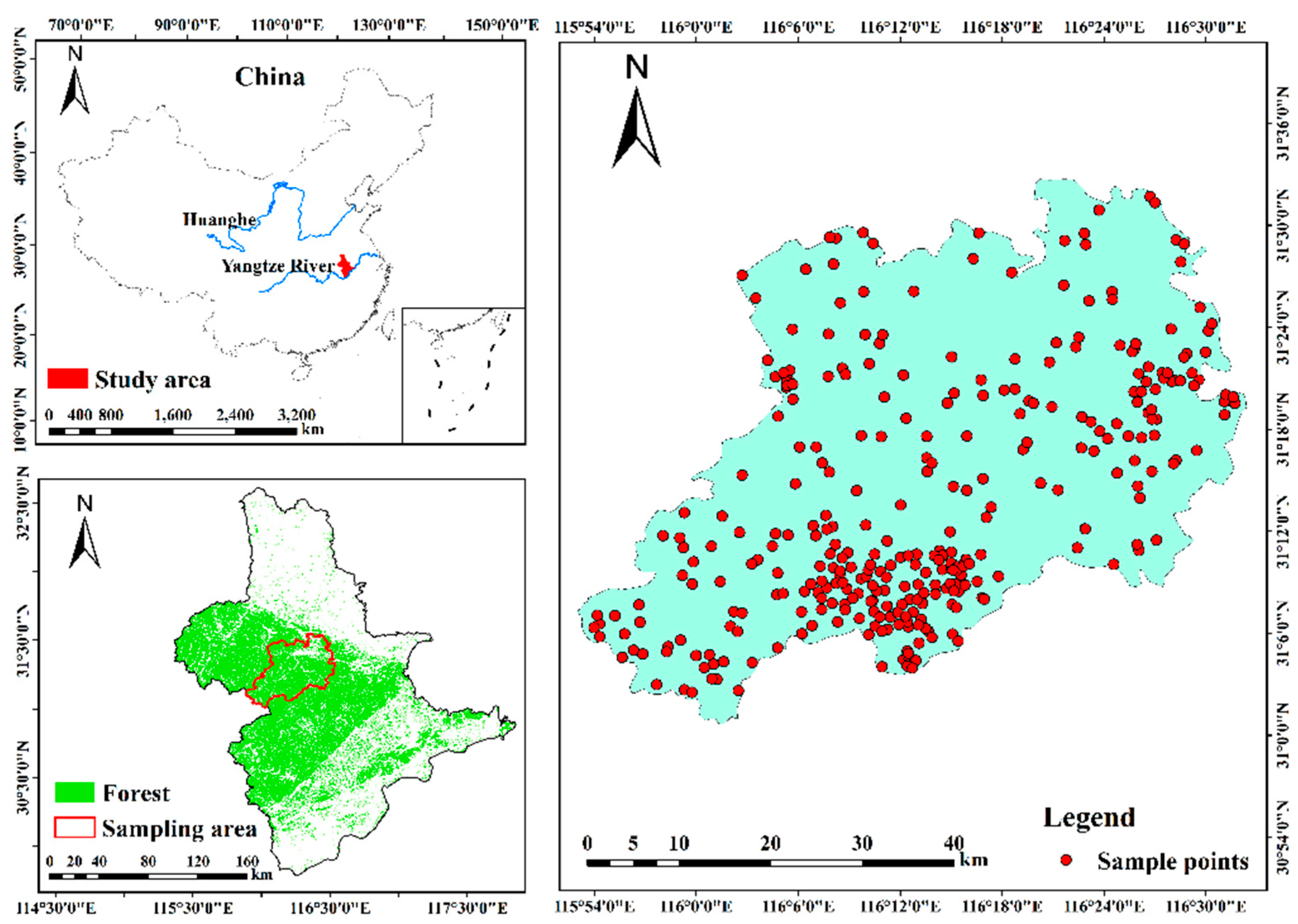
2.1. Study Area

The Dabie Mountains are located at the junction of Anhui, Hubei, and Henan provinces in China. The study area is the core component of the key ecological functional area of the Dabie Mountains (between 29.8°N–32.7°N and 115.4°E–117.8°E) (Figure 1) with an altitude of about 1000 m in general and some peaks exceeding 1500 m. The study area is located in the humid monsoon climate transitioning from the northern subtropical to the warm temperate zone, and it has a multi-year average temperature of 14.6–17.6 °C and an average annual precipitation of 1833 mm. The terrain of this region is complex, and can be roughly divided into middle mountains, low mountains, hills, and plains. The vegetation types mainly include broad-leaved forest, coniferous forest, coniferous and broad-leaved mixed forest, bamboo, and shrub, and the forest coverage is about 43.86%. Vegetation differentiation showed obvious vertical zonal characteristics because of the obvious vertical gradient change of habitat factors such as hydrothermal conditions. Cunninghamia lanceolata and Pinus massoniana forests are distributed below 400 to 600 m above sea level, while pine and broad-leaved species such as Pinus taiwanensis and Alnus trabeculosa are found mainly at 600 to 1200 m above sea level.

2.2. Data

2.2.1. Forest Inventory Data

This study utilized the forest inventory conducted at the county level by the Forest Management Inventory (FMI) in 2018. According to the technical regulations of FMI, the basic unit is the sub-compartment, which has basically the same internal characteristics and is significantly different from the adjacent units. In the assigned sub-compartment, setting up sample plots, recording the positions by GPS, and obtaining various survey factors in the sample plots are necessary. Each tree with the diameter at breast height (DBH) greater than 5 cm was measured, and indexes such as class number, ground class, dominant tree species, composition of tree species, forest age, tree height, and volume stock were recorded. The two-variable tree volume tables were looked up based on DBH and tree height, and all individual volume stocks were added up to form the total volume of stock in the plot. The sub-compartment area was determined according to the forest species, topographic map scale and management intensity used to draw the basic map. We pre-processed the collected forest inventory data, including information normalization, polygon removal, geographic registration, and small patch fusion. Sample plots were randomly generated from all sub-compartments, and the plots of non-forest land and plots with incomplete information were eliminated to form 326 sample plots (16 m × 16 m) (Figure 1).
This study used allometric equations [47,48] with the tree stock volume measured in field plots to map the AGB of broad-leaved forest, coniferous forest, and broad-leaved mixed forest. The allometric equation that describes the relationship between total volumes and the forest AGB of each sample plots is shown below:
B = a × V + b
where B is the aboveground biomass, measured in units of tons (t) per hectare (ha) (unit: t/ha); V is the average volume stock in each plot, measured in units of cubic meters (m3) per hectare (ha); and a, b are the function parameters (Table 1).
The AGB of the forest samples ranged from 9.23 t/ha to 205.54 t/ha, with average, median, and standard deviation (Std) values of 72.37, 80.64, and 28.52 t/ha, respectively, almost all of which were below 200 t/ha (Table 2). A total of 260 sample plots out of the 326 (80%) were randomly selected for training, and the remaining 66 plots (20%) were employed as validation datasets for the machine learning model.

2.2.2. Gaofen-1 WFV Image Pre-Processing and Variable Calculation

The GF1 optical satellite carries four wide-field-of-view (WFV) multispectral cameras, which provide a revisiting period of 4 days because of their wide field of view (800 km) [31]. GF1 WFV images from 3 May 2019, were downloaded from the China Centre for Resources Satellite Data and Application (http://36.112.130.153:7777/DSSPlatform/index.html (accessed on 10 December 2020)). The multispectral data with the spatial resolution of 16 m contains 4 spectral bands, namely, the band 1-blue (b1: 0.45–0.52 μm), band 2-green (b2: 0.52–0.59 μm), band 3-red (b3: 0.63–0.69 μm), and band 4-near-infrared (b4: 0.77–0.89 μm) spectra.
The GF1 images were pre-processed in ENVI software. The pre-processing steps mainly included radiation correction, atmospheric correction, orthorectification, mosaic, and clipping operation. Multispectral bands, including b1, b2, b3, and b4, and vegetation indexes (VI) (Table 3) were used as candidate factors to predict AGB. The gray level co-occurrence matrix (GLCM) was used to calculate the texture features, including the mean, variance, homogeneity, contrast, dissimilarity, entropy, second moment, and correlation features of b3 and b4 for each pixel with 3 × 3, 5 × 5, and 7 × 7 windows (e.g., b3_3Mean indicates the mean texture feature of band 3–red with a 3 × 3 window; the rest of the indicators were marked in the same way). A total of 59 variables were extracted from the high-resolution images (GF1) and used as input variables to participate in forest AGB estimation (Appendix A).

2.2.3. Sentinel-1 Data Pre-Processing and Variable Calculation

This research used the Sentinel-1 C-band SAR data of September 2019 downloaded from the Copernicus Open Access Hub of ESA (https://scihub.copernicus.eu/dhus/ (accessed on 15 June 2020)). The SAR data are available as high-resolution Level-1 Interferometric Wide Swath ground range detected processing level vertical transmit-horizontal receive (VH) and vertical transmit-vertical receive (VV) imagery with a pixel size of 10 m. The SNAP software was employed for pre-processing the S1 images. The pre-processing steps mainly included Thermal Noise Removal, Apply Orbit File, Calibration, Speckle Filter, Terrain Correction and Linear to Form dB. The processed images were resampled to 16 m pixel sizes to match with GF1 images. We extracted the VH and VV backscatter coefficients from the SAR images and calculated VH divided by VV as three variables. The GLCM was used to calculate the texture features of the VH and VV backscatter coefficients with a 3 × 3 window to develop the mapping of the AGB model parameters. A total of 19 variables were extracted from S1 images and further used as input variables to predict forest AGB (Appendix A).

2.2.4. Topographic Data and Preprocessing

The digital elevation model (DEM) reflects the abundant terrain information of the mountain region and provided great assistance to AGB estimation. DEM data with the resolution of 30 m were collected from USGS (https://earthexplorer.usgs.gov/ (accessed on 3 March 2021)). To ensure consistency with remote sensing-based data, the DEM data were resampled to 16 m resolution. Then, the altitude, slope, and aspect variables were extracted from the resampled results (Appendix A).

2.3. Methods

2.3.1. Stepwise Multiple Regression Algorithm

SMR is a type of multiple linear model. Through iteratively eliminating or adding variables to the regression model according to the partial regression square sum (significance) to obtain the optimal or appropriate fitting model, the SMR model helps analyze the linear relationships between multiple variables. In each iteration of selecting significant candidate variables or removing non-significant ones, the regression equation was evaluated by a significance test according to the p-value of an F statistic [35]. In the present study, the SMR model was implemented in SPSS software. During the operation, we set the AGB of the sample sites as the dependent variable and 81 variables extracted from remote sensing images and topographic data as the independent variables, and we selected the stepwise method. For “Probability of using F,” we set 0.05 and 0.1 to enter and remove, respectively.

2.3.2. Machine Learning Algorithms

Three types of MLAs, namely, SVM, RF, and backpropagation neural network (BPNN), were used to estimate forest AGB.
SVM has advantages in solving limited sample points and nonlinear and high-dimensional pattern problems. SVM identifies the optimum hyperplanes by using kernel functions to separate groups of input data with similar responses to predict a target variable [23]. We finally selected the radial basis function as the kernel function by 10-fold cross validation. To find the best parameters (e.g., gamma and C) for the model, we determined parameters within a certain range by performing a grid search 300 times. Here, the best parameters were gamma with 0.01 and C with 100.
RF is a non-parametric ensemble learning method based on bagging used for classification, regression, and other fields, and it has the capacity to efficiently process massive data and complex nonlinear relationships [45]. The RF algorithm is safe from information redundancy and over-fitting, and it has been successfully applied in AGB mapping. The RF model has two important parameters: the number of random trees (ntree) and the number of variables at the node (mtry). We posed 300 parameter sets and selected the ones with the highest accuracy. In this research, the ntree and mtry parameters were set as 232 and 4, respectively.
BPNN has a strong ability to fit the input data and provides a robust solution for complex and nonlinear problems between inputs and outputs metrics effectively [49]. BPNN includes an input layer, one or multiple hidden layers, and an output layer. The number of hidden layers and neurons are the two important parameters for building a neural network structure, which are examined repeatedly until the minimum root mean square error is achieved [50]. The number of hidden layers was set as 2, the neurons of the first layer was set as 4, and the neuron of the second layer was set as 2. BPNN is based on samples to achieve parameter estimation, and the accuracy also depends on the sample size.
We utilized the scikit-learn package in Python to develop and validate the above three machine learning models (http://scikit-learn.org/stable/ accessed on 26 October 2021) [51].

2.3.3. Performance Metrics

On the basis of the determination coefficient (R2), root mean square error (RMSE), mean absolute error (MAE), and mean error (ME), we evaluated the performance of the model in estimating AGB on the training and testing datasets.
RMSE = 1 n ( y i y ^ i ) 2 n
R 2 = 1 1 n ( y i y ^ i ) 2 1 n ( y i y ¯ i ) 2
MAE = 1 n y i y ^ i n
ME = 1 n ( y i y ^ i ) n
where y i is the sample point AGB values in the testing datasets, y ¯ i is the mean of y i , y ^ i is the predicted AGB values, i is the same index, and n is the number of testing samples.

2.3.4. Variable Selection

In this study, different variables were selected as input variables of the MLAs in multiple trials on the basis of correlation analysis. The performance of MLAs was evaluated based on R2, RMSE, MAE, and ME. Similar trials were conducted continuously, and a group of variables with the highest performance was eventually selected for AGB prediction in the study region.

3. Results

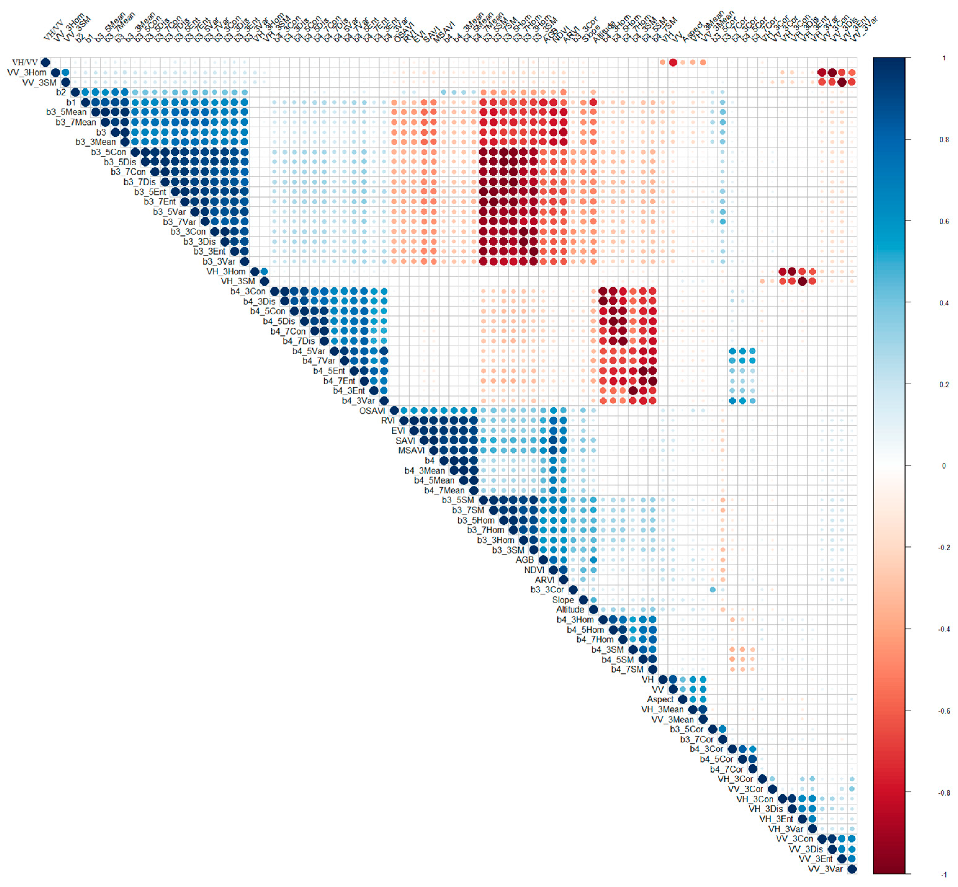
3.1. Relationships between Sample Point AGB and Variables

Pearson correlation analysis was used to analyze the relationships between 81 candidate variables derived from GF1, S1, and DEM data with sample point AGB values (Appendix A). Among the GF1 spectral variables, 47 were significantly related to field AGB values (p < 0.01), including multispectral bands (b1, b2, b3, b4), all the texture features of b3 with 3 × 3, 5 × 5, and 7 × 7 windows excluding b3_5Cor, all the texture features of b4 with the 7 × 7 window except for b4_7Cor, all the vegetation indices that had a positive correlation with AGB, and b4_3Hom, b4_3Mean, b4_5Con, b4_5Dis, b4_5Hom, and b4_5Mean (Table 4). Among them, NDVI, b1, b3_3Mean, b3, and b3_5Mean had the highest correlation with AGB (R = 0.674, −0.647, −0.615, −0.611, and −0.602, respectively). As for the S1 imagery, 4 candidate variables were significantly related to sample point AGB (p < 0.01), including two backscatter values (VH, VV), the 3 × 3 window size of VH_Mean and VV_Mean with R of 0.24, 0.188, 0.218, and 0.163. Among the variables extracted from DEM data, only altitude had a significantly positive correlation with field AGB.

3.2. Variable Combination and Model Construction

For the SMR model, the variable combination with the best performance (R2 = 0.56) for all sample plots included NDVI, altitude, b3_5SM, VH_3Mean, b3_7Ent, and b3_7Mean. The formula is summarized in Equation (6).
AGB= − 126.802 + 197.216 × NDVI + 0.019 × altitude + 38.411 × b3_5SM + 0.954 × VH_3Mean +10.445 × b3_7Ent − 2.303 × b3_7Mean (R2 = 0.564)
In this study, a series of trial results based on different variable permutations and combinations is listed in Table 5. Three MLAs produced different results under different combinations of variables with R2 ranging from 0.37 to 0.70, RMSE ranging from 16.26 t/ha to 23.60 t/ha, and MAE ranging from 12.80 t/ha to 17.47 t/ha. Considering the highest accuracy and the fewest variables, all MLAs achieved the highest accuracy under the variable combination of NDVI, MSAVI, b3_3Mean, b3_3Ent and altitude.

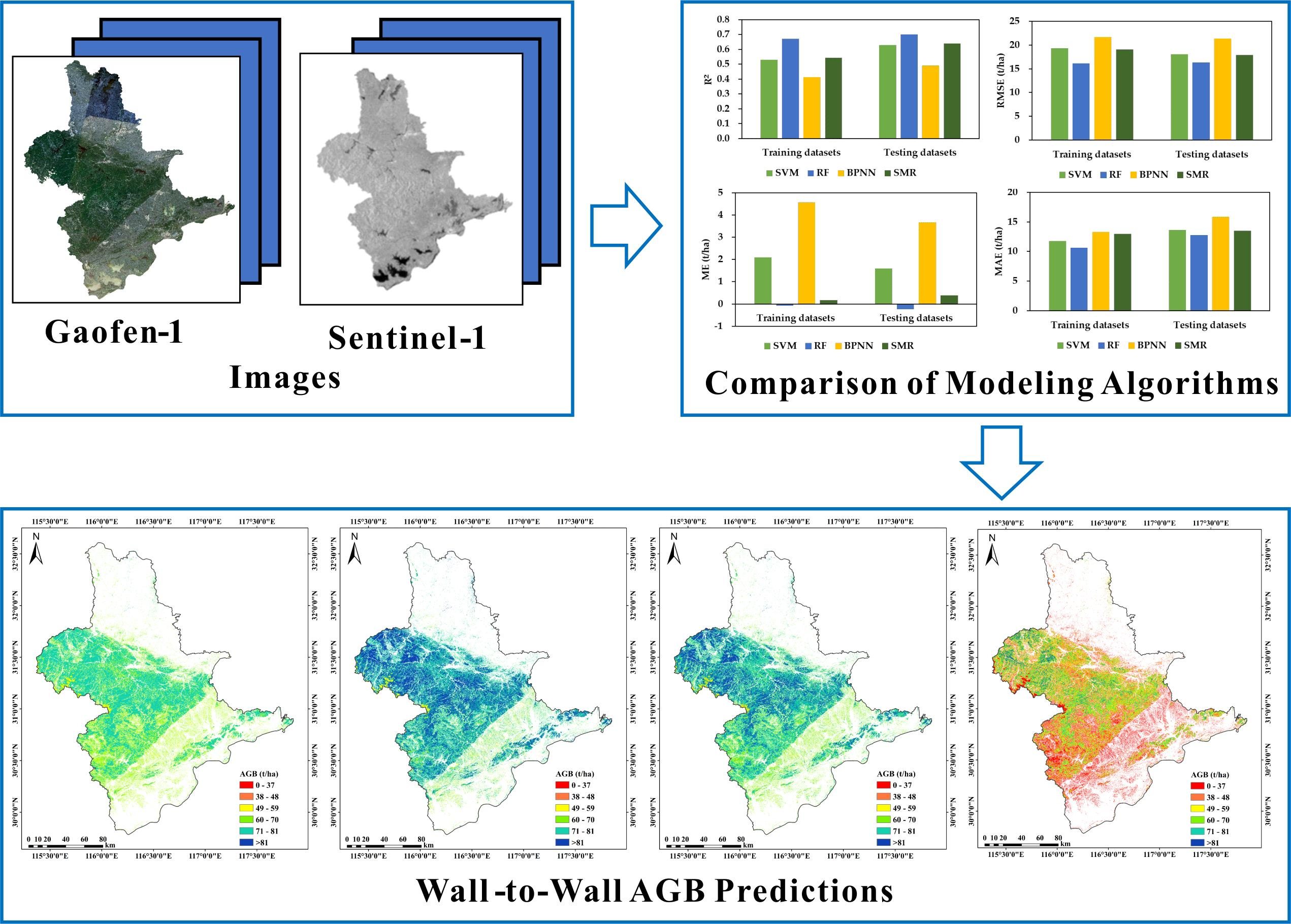
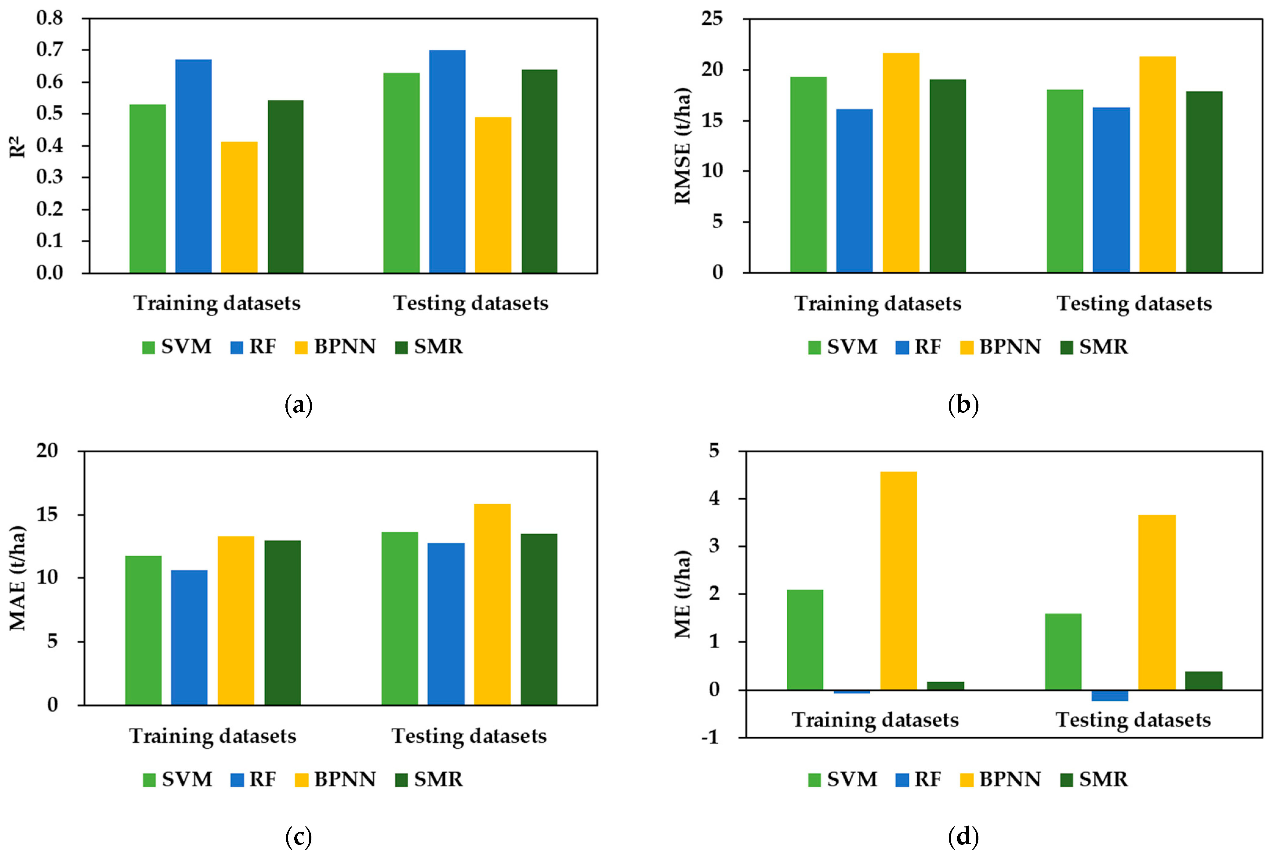
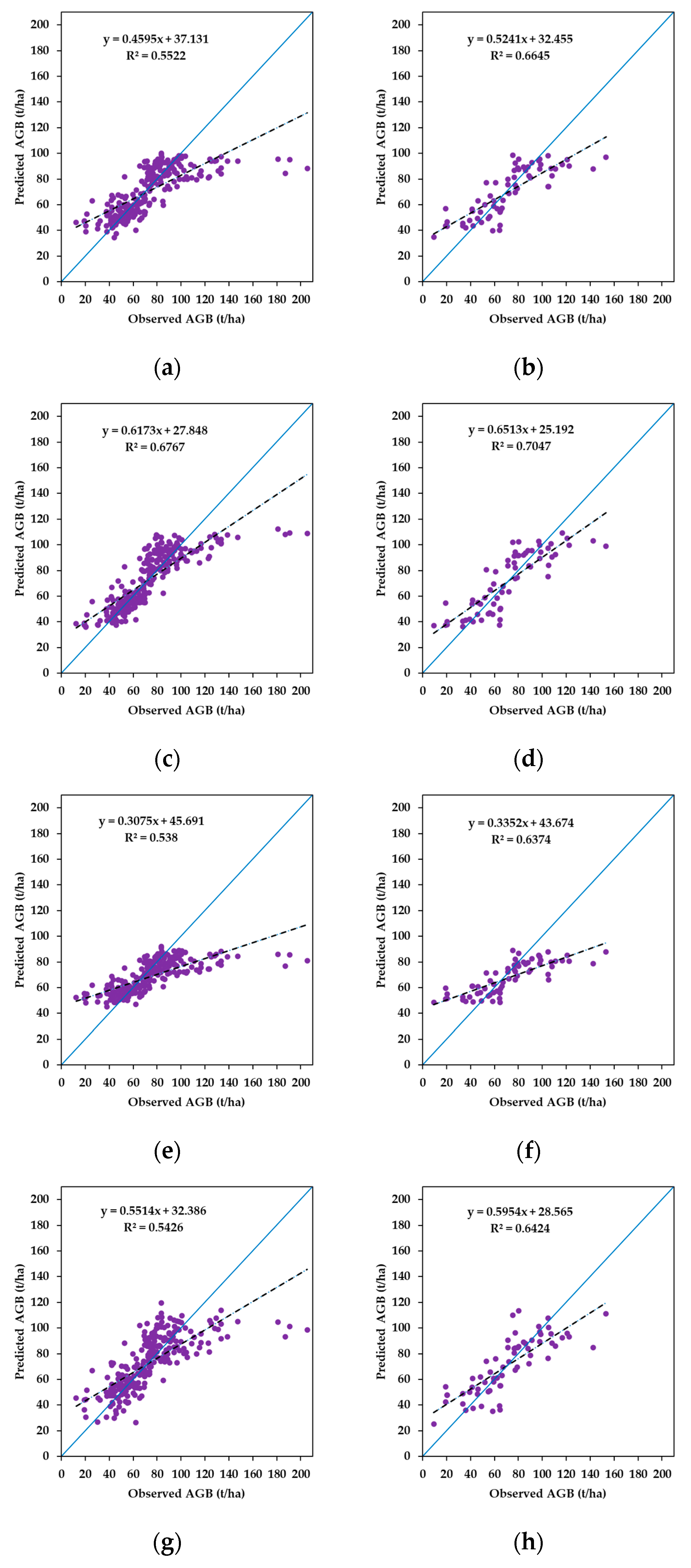
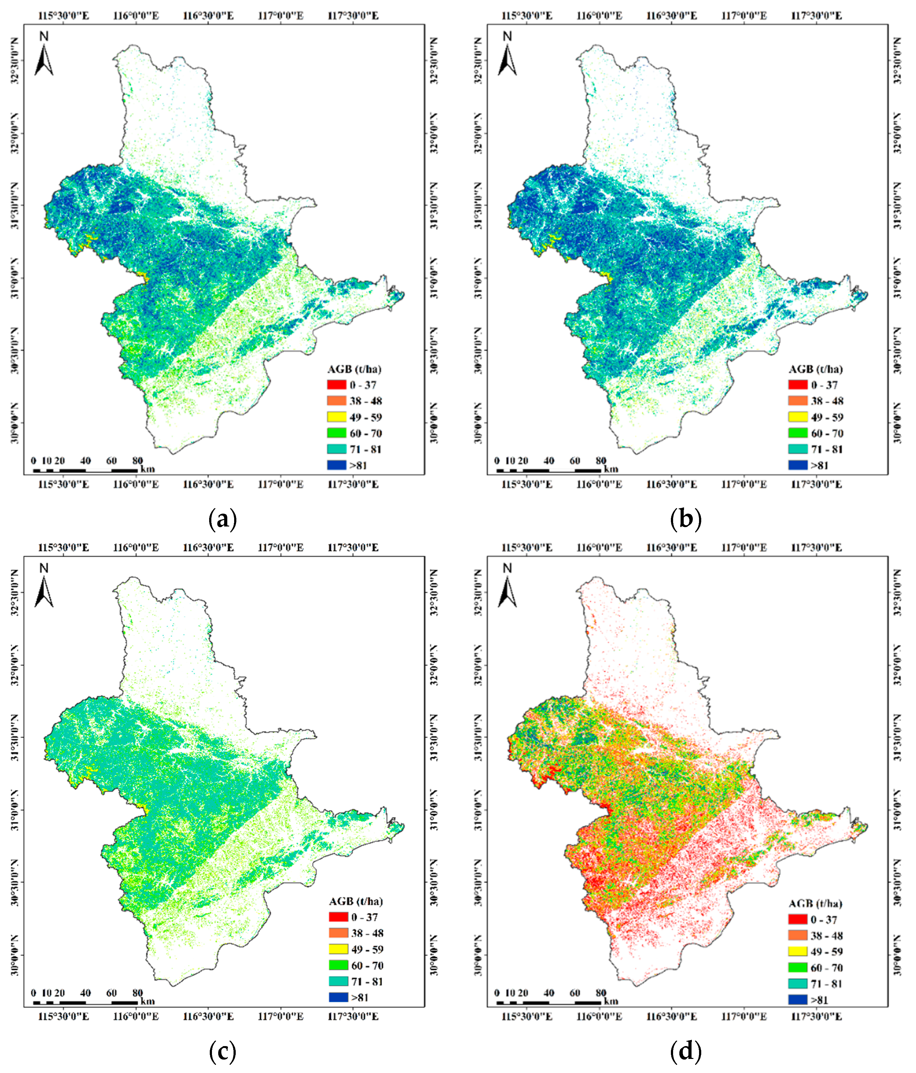
3.3. Comparison of the Estimated AGB Values among the Modeling Algorithms and Wall-to-Wall Predictions

The performance metrics of the SMR showed that the R2, RMSE, MAE and ME values were 0.64, 17.86, 13.53, and 0.39 t/ha in the training datasets, respectively, and the same values were 0.54, 19.08, 12.98, and 0.17 t/ha in the testing datasets, respectively (Figure 2). Among the MLAs, RF performed the best, with R2, RMSE, MAE, and ME of 0.67, 16.17, 10.63 and −0.08 t/ha, respectively, in the training datasets and R2 RMSE, MAE and ME of 0.70, 16.26, 12.80, and −0.24 t/ha, respectively, in the testing datasets. The performance of SVM was the second best, and the simulation result of BPNN in the two types of datasets was relatively poor. According to the ME values, the SMR, SVM, and BPNN models underestimated the forest AGB values.
Figure 3 shows the scatter plots of the SMR, SVM, RF, and BPNN algorithms for both the training and testing datasets. The results of the four models in the testing datasets were better than the accuracy of the training datasets, and the RF had the greatest accuracies (R2 is 0.68 in the training datasets; R2 is 0.70 in the testing datasets). Among the testing datasets, RF could explain 70% of the variance in the forest AGB, with the slope of 0.65. When the AGB was less than 39 t/ha, the RF model overestimated the values, and when the biomass is higher than 120 t/ha, the values were underestimated. A comparison of the results of the training datasets and the testing datasets shows that the accuracy of the RF model varied slightly, indicating the overfitting problem was not significant. The estimation result of SVM (R2 is 0.55 in the training datasets; R2 is 0.66 in the testing datasets) was lower than that of the RF model. In the testing datasets, the SVM model performed overestimation when AGB was less than 41 t/ha, and it underestimated AGB values above 100 t/ha. No major difference was found between the accuracies of SMR and SVM (R2 is 0.54 in the training datasets; R2 is 0.64 in the testing datasets), and the range of overestimation and underestimation was also similar. The BPNN model had a narrow estimation range of biomass with a flat slope (slope = 0.33). If the biomass was higher than 80 t/ha, then an underestimation is obtained, and the biomass was overestimated with low AGB values.
To compare the results of the modeling algorithms, different estimation results were divided into different numbers of categories to ensure the comparability of results in the same range (Figure 4). The minimum AGB values retrieved by the MLAs was about 38–49 t/ha, which was higher than the minimum value of the sample site (9.23 t/ha) and mainly distributed in the northern and southern towns, farmland, waters, and other nearby flat areas; the minimum values of the SMR were distributed at low values in the west. The high values retrieved by the four models were about 81–109 t/ha, which was lower than the highest biomass values of the sample site (205.54 t/ha). The high values were concentrated in the central, western, and southeast mountainous areas, forming a distinct distribution along the mountain range. A comparison of the results of forest biomass retrieval by different models showed that the average AGB values retrieved by the SVM, RF, BPNN, and SMR algorithms were 74.79, 78.17, 70.26, and 48.37 t/ha, respectively; the standard deviations were 7.55, 8.31, 4.95, and 19.56 t/ha, respectively. The mean biomass of SVM and RF was slightly higher than the mean biomass of the sample point (72.37 t/ha), and the SMR was much lower than the mean biomass of the sample point. Figure 4 indicates that the four modeling algorithms estimated forest AGB values with similar spatial patterns; that is, larger AGB values were spatially distributed in the west, central, and southeast parts of the study area, corresponding to the mountain region; smaller values were distributed in the south and southeast parts, and the values were scattered in the central part.

4. Discussion

4.1. Predictors of Forest AGB Mapping

The proper selection of predictors could improve the model performance and help understand the processes that resulted in the observed data. In this paper, the correlations between the extracted factors from GF1, S1 images, and topographic data with observed AGB values were examined, and numerous spectral variables have significant correlations with AGB. However, only a limited number of the remote sensing variables are selected for modeling AGB because of the high collinearity of spectral variables, and redundant input variables may introduce more errors that reduce the universality of the models [49,50]. To a certain extent, correlation analysis is helpful in eliminating the variables that cannot significantly improve AGB modeling accuracy. The random combination introduced in this article can help in adjusting the input variables, selecting the best combination of variables, and improving the AGB estimation accuracy.
Among the variables extracted by the GF1 imagery, NDVI is an important input predictor in both SMR and MLAs in the process of predicting AGB, which was also supported in previous research [23,52,53], and MSAVI is also widely used in AGB estimation in research. The performance of VIs can reflect green vegetation characteristics and improve biomass estimation accuracy. In addition, textural information refers to the pattern of intensity variations in remote sensing images, and it is efficient and effective in describing the spatial distribution and structure information of a forest [54,55]. Gao et al. [50] found that texture features may perform better than spectral factors in biomass estimation, especially in areas with multiple layers and complex forest stand structures. In this study, texture features calculated by spectral b3 were also applied in the modeling algorithm, where b3_3Mean and b3_3Ent were used in the MLAs, while b3_7Mean and b3_7Ent were used in the SMR model. As a result of the different features between the textural features and pixel-level spectral information, combinations of these variables can effectively capture the information of complex forest stand structures and can help improve AGB estimation. This finding is also consistent with previous studies [56].
The backscattering coefficient of the S1 imagery did not play a remarkably significant role in the model construction, which was similarly confirmed by Gao et al. [50], who found that ALOS PALSAR data performed more poorly than optical remote sensing data in AGB estimation for any applied modeling algorithms. This condition occurred because SAR data indicate the roughness of the forest canopy, which has a minimal impact on AGB prediction, while AGB was not directly related to the forest surface roughness [56]. Another study showed that SAR data make varying contributions to biomass in different quantity ranges, and when forest AGB values are lower than 130 t/ha, the SAR data have a weak effect [3]. In addition, S1 data are affected by interference of forest stand structures, underlying surface, and topography, thus producing inaccurate information for AGB estimation [57]. The topography and forest structures of the Dabie Mountain area are complex, thus causing the backscatter coefficient of SAR to be less sensitive to forest biomass than other interferences, resulting in the poor performance of AGB estimation.
Topographic features affect the composition of forest types and environmental conditions of growth (e.g., hydrothermal conditions, human disturbance), which could be indicated by the predicted AGB values in the Dabie Mountains. The AGB level was low in low-altitude areas such as towns, waters and other surrounding areas with high human accessibility. In contrast, the forest AGB values were high in high-altitude areas with low human accessibility. This finding indicates that topographic features were beneficial to AGB prediction.

4.2. Performance of Modeling Algorithms

The RF model is commonly applied and performs well in AGB prediction [45,58,59]. In this research, according to the performance metrics of the SMR and three MLAs, the RF model showed the best performance, with an R2 of 0.7, especially when the AGB values fell within 38–109 t/ha. As for the RF model, the fitting slope was close to 1, and the scattered points were more evenly distributed around the 1:1 line. Furthermore, the data range of the RF estimated values was the largest among the four models. The robust predicting capability of the RF model was also reported by Chen et al. [8]. The SVM model performed slightly more poorly than the RF model, followed by the SMR and BPNN models. The estimated AGB values of BPNN were mainly between 60 and 81 t/ha, and the values of the SMR model were generally less than 60 t/ha. With reference to the sample point data, the simulation result of the extreme values estimated by the four models was biased. There was underestimation in the high-value areas and overestimation in the low-value areas, which was mainly due to the limitations of optical and radar data saturation. For example, Gao et al. [50] found that models overestimated low AGB values and underestimated high AGB values because of the saturation problem when using Landsat TM and ALOS PALSAR data.
The biased AGB estimation with regards to extreme values could also be attributed to insufficient training samples. The average estimated AGB values of the modeling algorithms were close to the average measured AGB values of the sample points, with distinct overestimation and underestimation when it came to extreme high and low values. This situation may be related to the insufficient observations of sample point AGB values in the low and high ranges. Gao et al. [50] also indicated that extreme AGB values were the major factors that affected AGB modeling performance, and that collecting sufficient AGB sample plots with low or high value ranges could significantly improve AGB estimation accuracy. Selecting points from different levels of biomass sample points is particularly important to improving the prediction of very high or very low AGB values.

4.3. Limitations of Mapping AGB

The accuracy of assessing forest AGB may be subject to uncertain factors related to forest canopy structures, vegetation, topographic features, saturation problems, remote sensing images, and modeling algorithms [4,50,60]. Relevant studies confirmed that AGB estimation accuracy can be improved by optimizing the input model variables [8,11]. The present study considered textural features produced from GF1 images to participate in AGB prediction, and the finding was similar to the result of a previous study [56]. Li et al. [11] incorporated crown density with optical images to predict AGB values and increased the estimation accuracy. Zhu and Liu [53] used time series NDVI to improve the input parameters of AGB estimation. Gao et al. [50] found that using multi-source remote sensing images and model algorithms to evaluate different forest types could improve the accuracy of forest AGB estimation. The saturation problem of optical and radar images is unavoidable in the retrieval of biomass. A similar study also found that the saturation problem is a common issue in the estimation of the forest stock volume or biomass using multispectral remote sensing data [49]. At present, the problem of data saturation can be addressed by improving the spectral resolution and combining the data with LiDAR data. LiDAR data are more effective and robust in estimating biomass than hyperspectral data [22].
The uncertainty analysis of biomass estimation should be given more attention in the study of forest biomass estimation [3,58,61,62,63,64]. Su et al. [58] considered the impact of sample position offset on the uncertainty of biomass prediction. The representativeness of AGB values in sample plots is fundamental to AGB modeling, while sample plot data may be uncertain due to the sampling approach, plot size, allometric equations for AGB calculation, and measurements of tree attributes during fieldwork [50,56]. Zhang et al. [65] also reported the error caused by unrepresentative sample points in the uncertainty analysis of biomass retrieval, which produced uncertain factors for the retrieval of forest biomass [65]. Ahmed et al. [61] found that several allometric equations generally have estimation errors. In addition, plot size affects the biomass measurement accuracy of the sample points, and a large sample plot size indicates less error of the biomass measured at the sample points [66,67].
The RF model has the advantages of simpler operation, faster running speed, and ability to automatically assess and measure the importance of variables [68]. However, it also has obvious portability issues, which are affected by factors such as the quality of measured data, model algorithms, specific vegetation types, and environmental conditions. In this research, the RF model tended to generate a deviation within a low or high forest AGB value range.
In this study, the sample data did not match the time of the remote sensing images, and the influence of forest growth on the AGB estimation values was not considered. In a relatively short period of time, forest growth may not have a significant impact on the prediction of AGB in the whole study region, but for certain sample plots, the increase to AGB values within two years may not be negligible, resulting in the inability to accurately establish an AGB prediction model. Future work is necessary to supplement the inventory data of ground sample points on the time scale and to consider the influence of forest stratification to improve the current work of biomass estimation in the Dabie Mountains.

5. Conclusions

In this research, we selected the Dabie Mountain region in China as a case to explore the performance of MLAs and multi-source remote sensing-based data in estimating forest AGB. Through the trial comparison, five variables were selected as the input variables of the three MLAs to predict forest AGB, namely, remote sensing VIs (NDVI and MSAVI), texture features (b3_3Mean and b3_3Ent), and topographic variables (altitude). The conclusions include the following: (1) GF1 provided important spectral reflectance information for AGB estimation, especially for VIs and texture features; (2) the backscatter coefficient from the S1 images did not perform as well as input variables in constructing models, which may be due to SAR data being less sensitive to AGB than to the complexity of forest stand structures, underlying surface interference, and saturation problems; (3) among the four algorithms, RF was relatively the best and generally consistent with the AGB distribution of field plots in this study, indicating that nonparametric machine learning models have advantages in improving AGB estimation accuracy; and (4) the four modeling algorithms all have limited capability to estimate extremely high and low AGB values due to the saturation effect, limited training sample data, algorithm parameters, specific vegetation type, and environmental conditions. In sum, variable selection and model construction are the key factors for biomass estimation. Sufficient and representative sample points have positive effects on improving AGB estimation accuracy. Furthermore, the accuracy of forest AGB retrieved by remote sensing data still cannot fully meet the needs of accurate estimation of the carbon balance. The assimilation of multiple models and results estimated by remote sensing data is needed in future work.

Author Contributions

Conceptualization, R.W.; Funding acquisition, R.W.; Methodology, H.H.; Resources, B.L.; Supervision, R.W.; Writing—original draft, H.H.; Writing—review & editing, R.W. and B.L. All authors have read and agreed to the published version of the manuscript.

Funding

This study was financially supported by the Strategic Priority Research Program of the Chinese Academy of Sciences (Grant No. XDA23020201), National Natural Science Foundation of China (Grant Nos. 42071146, 41801092).

Institutional Review Board Statement

Not applicable.

Informed Consent Statement

Not applicable.

Data Availability Statement

Not applicable.

Conflicts of Interest

The authors declare no conflict of interest.

Appendix A

The correlation between 81 explanatory variables extracted from remote sensing images and topographic data and the response variable (forest AGB) is shown in Figure A1. Full names of the abbreviated variables involved in the manuscript are listed in Table A1.
Figure A1. Correlation coefficients between the forest AGB and the explanatory variables.
Remotesensing 14 00176 g0a1
Table A1. Variable abbreviation in correlation analysis.
Variable AbbreviationDescription
AGBforest aboveground biomass
b1band 1-blue
b2band 2-green
b3band 3-red
b4band 4 near-infrared
NDVINormalized Difference Vegetation Index
EVIEnhance Vegetation Index
RVIRatio Vegetation Index
ARVIAtmospherically Resistant Vegetation Index
SAVISoil Adjust Vegetation Index
MSAVIModified Soil Adjust Vegetation Index
OSAVIOptimized Soil Adjusted Vegetation Index
b3_3Concontrast of b3 with the 3 × 3 window
b3_3Corcorrelation of b3 with the 3 × 3 window
b3_3Dis dissimilarity of b3 with the 3 × 3 window
b3_3Ententropy of b3 with the 3 × 3 window
b3_3Hom homogeneity of b3 with the 3 × 3 window
b3_3Meanmean of b3 with the 3 × 3 window
b3_3SMsecond moment of b3 with the 3 × 3 window
b3_3Varvariance of b3 with the 3×3 window
b3_5Concontrast of b3 with the 5 × 5 window
b3_5Corcorrelation of b3 with the 5 × 5 window
b3_5Dis dissimilarity of b3 with the 5 × 5 window
b3_5Ententropy of b3 with the 5 × 5 window
b3_5Hom homogeneity of b3 with the 5 × 5 window
b3_5Meanmean of b3 with the 5 × 5 window
b3_5SMsecond moment of b3 with the 5 × 5 window
b3_5Varvariance of b3 with the 5 × 5 window
b3_7Concontrast of b3 with the 7 × 7 window
b3_7Corcorrelation of b3 with the 7 × 7 window
b3_7Dis dissimilarity of b3 with the 7 × 7 window
b3_7Ententropy of b3 with the 7 × 7 window
b3_7Hom homogeneity of b3 with the 7 × 7 window
b3_7Meanmean of b3 with the 7 × 7 window
b3_7SMsecond moment of b3 with the 7 × 7 window
b3_7Varvariance of b3 with the 7 × 7 window
b4_3Concontrast of b4 with the 3 × 3 window
b4_3Corcorrelation of b4 with the 3 × 3 window
b4_3Dis dissimilarity of b4 with the 3 × 3 window
b4_3Ententropy of b4 with the 3 × 3 window
b4_3Hom homogeneity of b4 with the 3 × 3 window
b4_3Meanmean of b4 with the 3 × 3 window
b4_3SMsecond moment of b4 with the 3 × 3 window
b4_3Varvariance of b4 with the 3 × 3 window
b4_5Concontrast of b4 with the 5 × 5 window
b4_5Corcorrelation of b4 with the 5 × 5 window
b4_5Dis dissimilarity of b4 with the 5 × 5 window
b4_5Ententropy of b4 with the 5 × 5 window
b4_5Hom homogeneity of b4 with the 5 × 5 window
b4_5Meanmean of b4 with the 5 × 5 window
b4_5SMsecond moment of b4 with the 5 × 5 window
b4_5Varvariance of b4 with the 5 × 5 window
b4_7Concontrast of b4 with the 7 × 7 window
b4_7Corcorrelation of b4 with the 7 × 7 window
b4_7Dis dissimilarity of b4 with the 7 × 7 window
b4_7Ententropy of b4 with the 7 × 7 window
b4_7Hom homogeneity of b4 with the 7 × 7 window
b4_7Meanmean of b4 with the 7 × 7 window
b4_7SMsecond moment of b4 with the 7 × 7 window
b4_7Varvariance of b4 with the 7 × 7 window
VHvertical transmit-horizontal receive
VVvertical transmit-vertical receive
VH/VVVH divided by VV
VH_3Concontrast of VH with the 3 × 3 window
VH_3Corcorrelation of VH with the 3 × 3 window
VH_3Dis dissimilarity of VH with the 3 × 3 window
VH_3Ententropy of VH with the 3 × 3 window
VH_3Hom homogeneity of VH with the 3 × 3 window
VH_3Meanmean of VH with the 3 × 3 window
VH_3SMsecond moment of VH with the 3 × 3 window
VH_3Varvariance of VH with the 3 × 3 window
VV_3Concontrast of VV with the 3 × 3 window
VV_3Corcorrelation of VV with the 3 × 3 window
VV_3Dis dissimilarity of VV with the 3 × 3 window
VV_3Ententropy of VV with the 3 × 3 window
VV_3Hom homogeneity of VV with the 3 × 3 window
VV_3Meanmean of VV with the 3 × 3 window
VV_3SMsecond moment of VV with the 3 × 3 window
VV_3Varvariance of VV with the 3 × 3 window
altitude-
slope-
aspect-

References

  1. Friedlingstein, P.; O’Sullivan, M.; Jones, M.W.; Andrew, R.M.; Hauck, J.; Olsen, A.; Peters, G.P.; Peters, W.; Pongratz, J.; Sitch, S. Global carbon budget 2020. Earth Syst. Sci. Data 2020, 12, 3269–3340. [Google Scholar] [CrossRef]
  2. Achard, F.; Eva, H.D.; Stibig, H.J.; Mayaux, P.; Gallego, J.; Richards, T.; Malingreau, J.P. Determination of deforestation rates of the world’s humid tropical forests. Science 2002, 297, 999–1002. [Google Scholar] [CrossRef] [Green Version]
  3. Huang, H.; Liu, C.; Wang, X.; Zhou, X.; Gong, P. Integration of multi-resource remotely sensed data and allometric models for forest aboveground biomass estimation in China. Remote Sens. Environ. 2019, 221, 225–234. [Google Scholar] [CrossRef]
  4. Ou, G.; Lv, Y.; Xu, H.; Wang, G. Improving Forest Aboveground Biomass Estimation of Pinus densata Forest in Yunnan of Southwest China by Spatial Regression using Landsat 8 Images. Remote Sens. 2019, 11, 2750. [Google Scholar] [CrossRef] [Green Version]
  5. Paul, K.I.; Roxburgh, S.H.; Chave, J.; England, J.R.; Zerihun, A.; Specht, A.; Lewis, T.; Bennett, L.T.; Baker, T.G.; Adams, M.A. Testing the generality of above-ground biomass allometry across plant functional types at the continent scale. Glob. Chang. Biol. 2016, 22, 2106–2124. [Google Scholar] [CrossRef] [PubMed]
  6. Paul, K.I.; Larmour, J.; Specht, A.; Zerihun, A.; Ritson, P.; Roxburgh, S.H.; Sochacki, S.; Lewis, T.; Barton, C.V.; England, J.R. Testing the generality of below-ground biomass allometry across plant functional types. For. Ecol. Manag. 2019, 432, 102–114. [Google Scholar] [CrossRef]
  7. Yu, X.; Ge, H.; Lu, D.; Zhang, M.; Lai, Z.; Yao, R. Comparative study on variable selection approaches in establishment of remote sensing model for forest biomass estimation. Remote Sens. 2019, 11, 1437. [Google Scholar] [CrossRef] [Green Version]
  8. Chen, L.; Wang, Y.; Ren, C.; Zhang, B.; Wang, Z. Optimal combination of predictors and algorithms for forest above-ground biomass mapping from Sentinel and SRTM data. Remote Sens. 2019, 11, 414. [Google Scholar] [CrossRef] [Green Version]
  9. Lu, D.; Chen, Q.; Wang, G.; Liu, L.; Li, G.; Moran, E. A survey of remote sensing-based aboveground biomass estimation methods in forest ecosystems. Int. J. Digit. Earth 2016, 9, 63–105. [Google Scholar] [CrossRef]
  10. Chave, J.; Davies, S.J.; Phillips, O.L.; Lewis, S.L.; Sist, P.; Schepaschenko, D.; Armston, J.; Baker, T.R.; Coomes, D.; Disney, M. Ground data are essential for biomass remote sensing missions. Surv. Geophys. 2019, 40, 863–880. [Google Scholar] [CrossRef]
  11. Li, C.; Li, Y.; Li, M. Improving forest aboveground biomass (AGB) estimation by incorporating crown density and using landsat 8 OLI images of a subtropical forest in Western Hunan in Central China. Forests 2019, 10, 104. [Google Scholar] [CrossRef] [Green Version]
  12. Wang, J.; Xiao, X.; Bajgain, R.; Starks, P.; Steiner, J.; Doughty, R.B.; Chang, Q. Estimating leaf area index and aboveground biomass of grazing pastures using Sentinel-1, Sentinel-2 and Landsat images. ISPRS J. Photogramm. Remote Sens. 2019, 154, 189–201. [Google Scholar] [CrossRef] [Green Version]
  13. Chen, Q.; McRoberts, R.E.; Wang, C.; Radtke, P.J. Forest aboveground biomass mapping and estimation across multiple spatial scales using model-based inference. Remote Sens. Environ. 2016, 184, 350–360. [Google Scholar] [CrossRef]
  14. Pham, T.D.; Yokoya, N.; Bui, D.T.; Yoshino, K.; Friess, D.A. Remote sensing approaches for monitoring mangrove species, structure, and biomass: Opportunities and challenges. Remote Sens. 2019, 11, 230. [Google Scholar] [CrossRef] [Green Version]
  15. Zhang, C.; Denka, S.; Cooper, H.; Mishra, D.R. Quantification of sawgrass marsh aboveground biomass in the coastal Everglades using object-based ensemble analysis and Landsat data. Remote Sens. Environ. 2018, 204, 366–379. [Google Scholar] [CrossRef]
  16. Foody, G.M.; Cutler, M.E.; Mcmorrow, J.; Pelz, D.; Tangki, H.; Boyd, D.S.; Douglas, I. Mapping the Biomass of Bornean Tropical Rain Forest from Remotely Sensed Data. Glob. Ecol. Biogeogr. 2001, 10, 379–387. [Google Scholar] [CrossRef]
  17. Main-Knorn, M.; Cohen, W.; Kennedy, R.; Grodzki, W.; Pflugmacher, D.; Griffiths, P.; Hostert, P. Monitoring coniferous forest biomass change using a Landsat trajectory-based approach. Remote Sens. Environ. 2013, 139, 277–290. [Google Scholar] [CrossRef]
  18. Pham, L.T.; Brabyn, L. Monitoring mangrove biomass change in Vietnam using SPOT images and an object-based approach combined with machine learning algorithms. ISPRS J. Photogramm. Remote Sens. 2017, 128, 86–97. [Google Scholar] [CrossRef]
  19. Englhart, S.; Keuck, V.; Siegert, F. Aboveground biomass retrieval in tropical forests—The potential of combined X-and L-band SAR data use. Remote Sens. Environ. 2011, 115, 1260–1271. [Google Scholar] [CrossRef]
  20. Cutler, M.E.J.; Boyd, D.S.; Foody, G.M.; Vetrivel, A. Estimating tropical forest biomass with a combination of SAR image texture and Landsat TM data: An assessment of predictions between regions. ISPRS J. Photogramm. Remote Sens. 2012, 70, 66–77. [Google Scholar] [CrossRef] [Green Version]
  21. Lefsky, M.A.; Cohen, W.B.; Harding, D.J.; Parker, G.G.; Acker, S.A.; Gower, S.T. Lidar remote sensing of above-ground biomass in three biomes. Glob. Ecol. Biogeogr. 2002, 11, 393–399. [Google Scholar] [CrossRef] [Green Version]
  22. Luo, S.; Wang, C.; Xi, X.; Pan, F.; Peng, D.; Zou, J.; Nie, S.; Qin, H. Fusion of airborne LiDAR data and hyperspectral imagery for aboveground and belowground forest biomass estimation. Ecol. Indic. 2017, 73, 378–387. [Google Scholar] [CrossRef]
  23. Zhang, L.; Shao, Z.; Liu, J.; Cheng, Q. Deep learning based retrieval of forest aboveground biomass from combined LiDAR and landsat 8 data. Remote Sens. 2019, 11, 1459. [Google Scholar] [CrossRef] [Green Version]
  24. Bortolot, Z.; Wynne, R. Estimating forest biomass using small footprint LiDAR data: An individual tree-based approach that incorporates training data. J. Photogramm. Remote Sens. 2005, 59, 342–360. [Google Scholar] [CrossRef]
  25. Cao, L.; Coops, N.; Innes, J.; Sheppard, S.; Fu, L.; Ruan, H.; She, G. Estimation of forest biomass dynamics in subtropical forests using multi-temporal airborne LiDAR data. Remote Sens. Environ. 2016, 178, 158–171. [Google Scholar] [CrossRef]
  26. Lin, Y.; West, G. Reflecting conifer phenology using mobile terrestrial LiDAR: A case study of Pinus sylvestris growing under the Mediterranean climate in Perth, Australia. Ecol. Indic. 2016, 70, 1–9. [Google Scholar] [CrossRef]
  27. Nie, S.; Wang, C.; Zeng, H.; Xi, X.; Li, G. Above-ground biomass estimation using airborne discrete-return and full-waveform LiDAR data in a coniferous forest. Ecol. Indic. 2017, 78, 221–228. [Google Scholar] [CrossRef]
  28. Qin, Y.; Li, S.; Vu, T.; Niu, Z.; Ban, Y. Synergistic application of geometric and radiometric features of LiDAR data for urban land cover mapping. Opt. Express 2015, 23, 13761–13775. [Google Scholar] [CrossRef] [PubMed]
  29. Sun, G.; Ranson, K.J.; Guo, Z.; Zhang, Z.; Montesano, P.; Kimes, D. Forest biomass mapping from lidar and radar synergies. Remote Sens. Environ. 2011, 115, 2906–2916. [Google Scholar] [CrossRef] [Green Version]
  30. Hudak, A.T.; Lefsky, M.A.; Cohen, W.B.; Berterretche, M. Integration of lidar and Landsat ETM+ data for estimating and mapping forest canopy height. Remote Sens. Environ. 2002, 82, 397–416. [Google Scholar] [CrossRef] [Green Version]
  31. Feng, L.; Li, J.; Gong, W.; Zhao, X.; Chen, X.; Pang, X. Radiometric cross-calibration of Gaofen-1 WFV cameras using Landsat-8 OLI images: A solution for large view angle associated problems. Remote Sens. Environ. 2016, 174, 56–68. [Google Scholar] [CrossRef]
  32. Fu, B.; Wang, Y.; Campbell, A.; Li, Y.; Zhang, B.; Yin, S.; Xing, Z.; Jin, X. Comparison of object-based and pixel-based Random Forest algorithm for wetland vegetation mapping using high spatial resolution GF-1 and SAR data. Ecol. Indic. 2017, 73, 105–117. [Google Scholar] [CrossRef]
  33. Minh, D.H.T.; Ndikumana, E.; Vieilledent, G.; McKey, D.; Baghdadi, N. Potential value of combining ALOS PALSAR and Landsat-derived tree cover data for forest biomass retrieval in Madagascar. Remote Sens. Environ. 2018, 213, 206–214. [Google Scholar] [CrossRef]
  34. Zhang, L.; Shao, Z.; Diao, C. Synergistic retrieval model of forest biomass using the integration of optical and microwave remote sensing. J. Appl. Remote Sens. 2015, 9, 096069. [Google Scholar] [CrossRef]
  35. Li, L.; Zhou, X.; Chen, L.; Chen, L.; Zhang, Y.; Liu, Y. Estimating urban vegetation biomass from Sentinel-2A image data. Forests 2020, 11, 125. [Google Scholar] [CrossRef] [Green Version]
  36. McRoberts, R.E. Estimating forest attribute parameters for small areas using nearest neighbors techniques. For. Ecol. Manag. 2012, 272, 3–12. [Google Scholar] [CrossRef]
  37. Rodríguez-Veiga, P.; Quegan, S.; Carreiras, J.; Persson, H.J.; Fransson, J.E.; Hoscilo, A.; Ziółkowski, D.; Stereńczak, K.; Lohberger, S.; Stängel, M. Forest biomass retrieval approaches from earth observation in different biomes. Int. J. Appl. Earth Obs. Geoinf. 2019, 77, 53–68. [Google Scholar] [CrossRef]
  38. Tian, X.; Yan, M.; van der Tol, C.; Li, Z.; Su, Z.; Chen, E.; Li, X.; Li, L.; Wang, X.; Pan, X. Modeling forest above-ground biomass dynamics using multi-source data and incorporated models: A case study over the qilian mountains. Agric. For. Meteorol. 2017, 246, 1–14. [Google Scholar] [CrossRef]
  39. Mas, J.; Flores, J. The application of artificial neural networks to the analysis of remotely sensed data. Int. J. Remote Sens. 2008, 29, 617–663. [Google Scholar] [CrossRef]
  40. Szantoi, Z.; Escobedo, F.J.; Abd-Elrahman, A.; Pearlstine, L.; Dewitt, B.; Smith, S. Classifying spatially heterogeneous wetland communities using machine learning algorithms and spectral and textural features. Environ. Monit. Assess. 2015, 187, 262. [Google Scholar] [CrossRef]
  41. Breiman, L. Random forests. Mach. Learn. 2001, 45, 5–32. [Google Scholar] [CrossRef] [Green Version]
  42. KopeĿ, D.; Michalska-Hejduk, D.; Berezowski, T.; Borowski, M.; Rosadziſski, S.; Chormaſski, J. Application of multisensoral remote sensing data in the mapping of alkaline fens Natura 2000 habitat. Ecol. Indic. 2016, 70, 196–208. [Google Scholar] [CrossRef]
  43. Pal, M. Random forest classifier for remote sensing classification. Int. J. Remote Sens. 2005, 26, 217–222. [Google Scholar] [CrossRef]
  44. Wan, R.; Wang, P.; Wang, X.; Yao, X.; Dai, X. Mapping aboveground biomass of four typical vegetation types in the Poyang Lake wetlands based on random forest modelling and landsat images. Front. Plant Sci. 2019, 10, 1281. [Google Scholar] [CrossRef]
  45. Zeng, N.; Ren, X.; He, H.; Zhang, L.; Zhao, D.; Ge, R.; Li, P.; Niu, Z. Estimating grassland aboveground biomass on the Tibetan Plateau using a random forest algorithm. Ecol. Indic. 2019, 102, 479–487. [Google Scholar] [CrossRef]
  46. Mountrakis, G.; Im, J.; Ogole, C. Support vector machines in remote sensing: A review. ISPRS J. Photogramm. Remote Sens. 2011, 66, 247–259. [Google Scholar] [CrossRef]
  47. Fang, J.; Chen, A. Dynamic forest biomass carbon pools in China and their significance. J. Integr. Plant Biol. 2001, 43, 967–973. [Google Scholar]
  48. Fang, J.; Liu, G.; Xu, S. Biomass and net production of Forest vegetation in China. Acta Ecol. Sin. 1996, 16, 497–508. [Google Scholar]
  49. Ou, G.; Li, C.; Lv, Y.; Wei, A.; Xiong, H.; Xu, H.; Wang, G. Improving aboveground biomass estimation of Pinus densata forests in Yunnan using Landsat 8 imagery by incorporating age dummy variable and method comparison. Remote Sens. 2019, 11, 738. [Google Scholar] [CrossRef] [Green Version]
  50. Gao, Y.; Lu, D.; Li, G.; Wang, G.; Chen, Q.; Liu, L.; Li, D. Comparative analysis of modeling algorithms for forest aboveground biomass estimation in a subtropical region. Remote Sens. 2018, 10, 627. [Google Scholar] [CrossRef] [Green Version]
  51. Pedregosa, F.; Varoquaux, G.; Gramfort, A.; Michel, V.; Thirion, B.; Grisel, O.; Blondel, M.; Prettenhofer, P.; Weiss, R.; Dubourg, V. Scikit-learn: Machine learning in Python. J. Mach. Learn. Res. 2011, 12, 2825–2830. [Google Scholar]
  52. Hu, Y.; Xu, X.; Wu, F.; Sun, Z.; Xia, H.; Meng, Q.; Huang, W.; Zhou, H.; Gao, J.; Li, W. Estimating forest stock volume in Hunan Province, China, by integrating in situ plot data, Sentinel-2 images, and linear and machine learning regression models. Remote Sens. 2020, 12, 186. [Google Scholar] [CrossRef] [Green Version]
  53. Zhu, X.; Liu, D. Improving forest aboveground biomass estimation using seasonal Landsat NDVI time-series. ISPRS J. Photogramm. Remote Sens. 2015, 102, 222–231. [Google Scholar] [CrossRef]
  54. Haralick, R. Statistical and structural approaches to texture. Proc. IEEE 1979, 67, 786–804. [Google Scholar] [CrossRef]
  55. Sarker, L.R.; Nichol, J.E. Improved forest biomass estimates using ALOS AVNIR-2 texture indices. Remote Sens. Environ. 2011, 115, 968–977. [Google Scholar] [CrossRef]
  56. Zhao, P.; Lu, D.; Wang, G.; Liu, L.; Li, D.; Zhu, J.; Yu, S. Forest aboveground biomass estimation in Zhejiang Province using the integration of Landsat TM and ALOS PALSAR data. Int. J. Appl. Earth Obs. Geoinf. 2016, 53, 1–15. [Google Scholar] [CrossRef]
  57. Fayad, I.; Baghdadi, N.; Guitet, S.; Bailly, J.; Hérault, B.; Gond, V.; El Hajj, M.; Minh, D. Aboveground biomass mapping in French Guiana by combining remote sensing, forest inventories and environmental data. Int. J. Appl. Earth Obs. Geoinf. 2016, 52, 502–514. [Google Scholar] [CrossRef] [Green Version]
  58. Su, Y.; Guo, Q.; Xue, B.; Hu, T.; Alvarez, O.; Tao, S.; Fang, J. Spatial distribution of forest aboveground biomass in China: Estimation through combination of spaceborne lidar, optical imagery, and forest inventory data. Remote Sens. Environ. 2016, 173, 187–199. [Google Scholar] [CrossRef] [Green Version]
  59. Wan, R.; Wang, P.; Wang, X.; Yao, X.; Dai, X. Modeling wetland aboveground biomass in the Poyang Lake National Nature Reserve using machine learning algorithms and Landsat-8 imagery. J. Appl. Remote Sens. 2018, 12, 046029. [Google Scholar] [CrossRef]
  60. Zhao, P.; Lu, D.; Wang, G.; Wu, C.; Huang, Y.; Yu, S. Examining spectral reflectance saturation in Landsat imagery and corresponding solutions to improve forest aboveground biomass estimation. Remote Sens. 2016, 8, 469. [Google Scholar] [CrossRef] [Green Version]
  61. Ahmed, R.; Siqueira, P.; Hensley, S.; Bergen, K. Uncertainty of forest biomass estimates in north temperate forests due to allometry: Implications for remote sensing. Remote Sens. 2013, 5, 3007–3036. [Google Scholar] [CrossRef] [Green Version]
  62. Chen, Q.; Laurin, G.; Valentini, R. Uncertainty of remotely sensed aboveground biomass over an African tropical forest: Propagating errors from trees to plots to pixels. Remote Sens. Environ. 2015, 160, 134–143. [Google Scholar] [CrossRef]
  63. Fleming, A.L.; Wang, G.; McRoberts, R.E. Comparison of methods toward multi-scale forest carbon mapping and spatial uncertainty analysis: Combining national forest inventory plot data and landsat TM images. Eur. J. For. Res. 2015, 134, 125–137. [Google Scholar] [CrossRef]
  64. Mascaro, J.; Detto, M.; Asner, G.P.; Muller-Landau, H.C. Evaluating uncertainty in mapping forest carbon with airborne LiDAR. Remote Sens. Environ. 2011, 115, 3770–3774. [Google Scholar] [CrossRef]
  65. Zhang, G.; Ganguly, S.; Nemani, R.R.; White, M.A.; Milesi, C.; Hashimoto, H.; Wang, W.; Saatchi, S.; Yu, Y.; Myneni, R.B. Estimation of forest aboveground biomass in California using canopy height and leaf area index estimated from satellite data. Remote Sens. Environ. 2014, 151, 44–56. [Google Scholar] [CrossRef]
  66. Frazer, G.; Magnussen, S.; Wulder, M.; Niemann, K. Simulated impact of sample plot size and co-registration error on the accuracy and uncertainty of LiDAR-derived estimates of forest stand biomass. Remote Sens. Environ. 2011, 115, 636–649. [Google Scholar] [CrossRef]
  67. Ruiz, L.A.; Hermosilla, T.; Mauro, F.; Godino, M. Analysis of the influence of plot size and LiDAR density on forest structure attribute estimates. Forests 2014, 5, 936–951. [Google Scholar] [CrossRef] [Green Version]
  68. Mutanga, O.; Adam, E.; Cho, M.A. High density biomass estimation for wetland vegetation using WorldView-2 imagery and random forest regression algorithm. Int. J. Appl. Earth Obs. Geoinf. 2012, 18, 399–406. [Google Scholar] [CrossRef]
Figure 1. Location of the study area and the distribution of sampling points.
Remotesensing 14 00176 g001
Figure 2. Performance metrics of the four models in estimating AGB: (a) R2, (b) RMSE, (c) MAE, (d) ME.
Remotesensing 14 00176 g002
Figure 3. Scatter plots of the four models in estimating AGB in the training datasets (left) and testing datasets (right): (a,b) SVM, (c,d) RF, (e,f) BPNN, and (g,h) SMR.
Remotesensing 14 00176 g003
Figure 4. AGB estimation retrieved by the four modeling algorithms: (a) SVM, (b) RF, (c) BPNN, and (d) SMR.
Remotesensing 14 00176 g004
Table 1. Parameters a and b for calculating forest aboveground biomass [48].
Forest TypeabSample Size (ind)R2
Picea, Abies0.464247.4990130.98
Hemlock, Cryptomeria, Keteleeria0.415841.3318210.94
Betula0.96440.848540.98
Poplar0.475430.6034100.93
Camphor forest, Phoebe1.03578.0591170.91
Cunninghamia Lanceolata0.399922.5410560.97
Cypress0.612926.1451110.98
Quercus1.14538.5473120.98
Eucalyptus0.88734.5539200.80
Larix0.609633.8060340.82
Pinus armandii Franch0.585618.743590.91
Pinus massoniana0.503420.547520.87
Chinese pine0.75545.0928820.98
Other pinus0.516833.2378190.86
Hard broadleaf forest1.17832.5585170.95
Soft broadleaf forest0.475430.603160.92
Coniferous and broadleaf mixed forest0.813618.466100.99
Table 2. The statistics of AGB in training, testing, and total sample datasets.
Sample Size (ind)Min (t/ha)Max(t/ha)Mean(t/ha)Median(t/ha)Std(t/ha)
Training26012.33205.5472.5778.7528.21
Testing669.23153.2071.5767.5729.72
Total3269.23205.5472.3780.6428.52
Table 3. Vegetation indices and their calculation formula.
Vegetation IndicesFormula
NDVI NIR     R NIR   +   R
RVI NIR R
EVI 2.5   ×   ( NIR     R ) 1   +   NIR   +   6   ×   R     7.5   ×   B
ARVI NIR     ( 2   ×   R     B ) NIR   +   ( 2   ×   R     B )
SAVI ( 1   +   0.5 ) NIR     R NIR   +   R   +   0.5
MSAVI NIR   +   0.5     ( ( NIR   +   0.5 ) 2     2   ×   ( NIR     R ) ) 1 2
OSAVI ( 1   +   0.16 ) ( NIR     R ) ( NIR   +   R   +   0.16 )
Table 4. Variables significantly associated with forest aboveground biomass.
VariablesCorrelation
Coefficients
VariablesCorrelation CoefficientsVariablesCorrelation
Coefficients
VariablesCorrelation
Coefficients
NDVI+0.674 **MSAVI+0.544 **b4_3Mean+0.387 **b3_3Cor+0.209 **
b1−0.647 **altitude +0.544 **b4_5Mean+0.383 **b4_7Hom+0.193 **
b3_3Mean−0.615 **ARVI+0.537 **b4_7Mean+0.378 **b4_7Dis−0.188 **
b3−0.611 **b3_5Hom+0.486 **b2−0.339 **VV+0.188 **
b3_5Mean−0.602 **b3_7Hom+0.485 **b3_3Con−0.288 **b4_7Ent−0.179 **
b3_7Mean−0.579 **b3_3Hom+0.478 **b3_7Cor−0.275 **b4_5Hom+0.175 **
b3_5SM+0.566 **RVI+0.441 **b3_7Var−0.27 **b4_7Var−0.173 **
b3_3SM+0.56 **EVI+0.441 **b3_7Con−0.26 **b4_5Dis−0.168 **
b3_5Ent−0.56 **b3_3Dis−0.416 **b3_5Con−0.259 **b4_7Con−0.168 **
b3_7SM+0.554 **OSAVI+0.404 **VH+0.24 **VV_3Mean+0.163 **
SAVI+0.553 **b3_5Dis−0.403 **b3_5Var−0.235 **b4_3Hom+0.152 **
b3_7Ent−0.551 **b3_7Dis−0.402 **VH_3Mean+0.218 **b4_5Con−0.15 **
b3_3Ent−0.55 **b4+0.388 **b3_3Var−0.211 **b4_7SM+0.146 **
b3_3Con, b3_3Cor, b3_3Dis, b3_3Ent, b3_3Hom, b3_3Mean, b3_3SM, and b3_3Var indicate the contrast, correlation, dissimilarity, entropy, homogeneity, mean, second moment, and variance texture features of band 3-red with the 3 × 3 window, respectively. The rest of the indicators can be marked in the same way. ** indicates a significance level of 0.01.
Table 5. Trial results of variable combinations.
VariablesModelR2RMSEMAEME
NDVI, b1, b3, b3_3Mean, b3_5Mean, b3_7Mean, altitudeSVM0.5819.2014.501.69
RF0.6517.5113.93−0.98
BPNN0.4821.3315.742.34
NDVI, b1, b3, b3_3Mean, b3_5Mean, b3_7MeanSVM0.5320.4014.922.22
RF0.6118.5914.55−1.10
BPNN0.4222.6016.871.91
NDVI, ARVI, MSAVI, b1, b3SVM0.5619.6614.332.06
RF0.6118.5814.36−1.22
BPNN0.3723.6017.475.75
NDVI, MSAVI, b3, b3_3Mean, b3_3Ent, altitude, VV_3MeanSVM0.6018.8114.211.33
RF0.6717.1613.15−0.38
BPNN0.4621.8316.264.61
NDVI, MSAVI, b3, b3_3Mean, b3_3Ent, altitudeSVM0.6218.2913.761.42
RF0.7016.3712.81−0.24
BPNN0.5120.7915.513.56
NDVI, MSAVI, b3, b3_3Mean, altitudeSVM0.5819.1614.482.39
RF0.6816.8313.31−0.50
BPNN0.4821.4515.853.22
NDVI, MSAVI, b3_3Mean, b3_3Ent, altitudeSVM0.6618.0313.651.60
RF0.7016.2612.80−0.24
BPNN0.4921.3015.863.66
NDVI, MSAVI, b3_5Con, b3_5Dis, altitudeSVM0.6118.3414.090.04
RF0.6617.2413.210.30
BPNN0.4821.4415.873.00
NDVI, MSAVI, b3_3Mean, b3_5Con, altitudeSVM0.5819.1814.232.24
RF0.6916.6712.900.10
BPNN0.4921.3015.723.42
NDVI, MSAVI, b3_7Mean, b3_7Ent, altitudeSVM0.6218.2113.841.84
RF0.6617.4413.70−0.49
BPNN0.4721.6116.094.61
……
Publisher’s Note: MDPI stays neutral with regard to jurisdictional claims in published maps and institutional affiliations.

