Abstract
The cloud-top-phase climatology over the western North Pacific (WNP) has received little attention. Using 3 years (2017–2019) of cloud-top-phase products from the Advanced Himawari Imager onboard the Japanese Himawari-8 satellite, this study examines the seasonal and diurnal variations in the cloud-top phase over the WNP. Results show that over the low- and mid-latitude maritime regions, ice (water) clouds occur more (less) frequently during boreal winter than summer. Water clouds are more likely to be related to moisture conditions in the lower troposphere than to the underlying sea surface temperature. Owing to the combined effects of moist air mass transport and ocean currents (topography), the WNP region east of Hokkaido (the Sichuan Basin) has a high frequency of water clouds in summer (winter). Furthermore, supercooled water cloud populations have a clear seasonal cycle. The fraction of water clouds that are supercooled appears to be modulated by the near-surface air temperature. A diurnal cycle is seen in ice-cloud populations, which are highest in the late afternoon over both ocean and land except for the Sichuan Basin where summer nocturnal precipitation is typical. The occurrences of continental water clouds peak at noon in summer but early morning (around sunrise) in winter. An increase in the frequency of continental summer water clouds around noon is found to be associated with variations in both the cloud-top elevation of already-existing water clouds and new formations of boundary-layer clouds.
1. Introduction
The cloud thermodynamic phase (or simply, cloud phase) indicates whether cloud particles consist of ice crystals, water droplets, or a mixture of both. It is important to know the cloud phase for determining the role of clouds in regulating Earth’s hydrological cycle and radiative budget. First, according to the “ice crystal precipitation” theory [1], ice crystals in a mixed-phase cloud grow at the expense of the supercooled water droplets. Precipitation starts when the ice crystals grow to sufficient sizes. Thus, the ice phase controls the development of precipitation and affects the lifetime of clouds [2]. Second, water (ice) clouds reflect more (less) incoming shortwave solar radiation than they absorb outgoing infrared terrestrial radiation, resulting in negative (positive) net radiative heating [3,4]. The net cloud phase feedback depends on the amount and fraction of cloud water and ice. Therefore, an accurate representation of the cloud phase is essential for understanding and modeling cloud–precipitation–climate interactions and reducing the uncertainty in weather and climate predictions.
The reflected shortwave radiation in the Southern Ocean (SO) region, including the southern reaches of the Pacific, Indian, and Atlantic oceans, is found to be significantly underestimated in global climate models [5,6,7], higher-resolution regional models [8,9], and state-of-the-art reanalysis [10]. Previous studies have suggested that underestimates of the fractions and optical depths of low- and mid-altitude clouds [11,12] and an overestimate of the occurrence frequency of drizzle [13] greatly contribute to the model biases in reflected shortwave radiation. Using observations from modern passive and active instruments onboard the A-train constellation of satellites [14], the thermodynamic and microphysical structures of SO clouds have been extensively investigated. Huang et al. [15] found that low-altitude clouds are dominant over the SO region year-round with little seasonality, conflicting with the clear seasonal cycle of the model biases in radiative flux simulations [16]. However, all studies have shown the extensive presence of supercooled water clouds across this region, especially during austral summer [9,15,17,18,19]. The meteorological community has now accepted that climate models show large biases over the SO region mainly due to their inability to represent the prevalence of supercooled water clouds [2,20], highlighting the importance and necessity of having a cloud-top-phase climatology.
The cloud-top-phase climatology of the western North Pacific (WNP) has received little attention compared with that of the SO, even though it covers a larger area of Earth’s surface. Pioneering studies [18,21] have consistently focused on extratropical cyclones that create storm tracks, a phenomenon that frequently occurs over the mid-latitude ocean. Mace [22] compared the cloud properties of mid-latitude storm-track systems over the SO and the North Atlantic and concluded that cloud-occurrence statistics and cloud properties have a “high degree of similarity” in the two regions. This conclusion is remarkable and set the tone for the climatology of cloud-top phase over the Northern Hemisphere, perhaps dimming subsequent studies. In fact, the surface forcing in the SO and WNP regions is not completely consistent. In the WNP, the oceanic heat transport is easily affected by continental barriers, so the sea surface temperature (SST) shows an obvious east–west gradient. In the SO, where the ocean currents are mainly zonal, a north–south SST gradient dominates. The dependence of the cloud-top phase on the underlying SST, found by [20,23], suggests that the cloud-top-phase distributions of the two regions may be measurably different. Another expected difference between the SO and the WNP is the atmospheric stability. Using the products of NASA’s Modern-Era Retrospective Analysis for Research and Applications [24], Naud et al. [21] examined the differences in synoptic environments for extratropical cyclones over the Southern and Northern Hemispheres. They found that poleward transports of moisture are more vigorous in the Northern Hemisphere than in the Southern Hemisphere. In addition to the abovementioned two differences, the WNP is more affected by trans-ocean aerosols than the SO, especially during the spring [25,26]. Trans-Pacific aerosols, including natural and anthropogenic ones, are emitted in Central and East Asia, lifted into the mid- and upper troposphere, and then transported by the westerlies to North American regions [27]. These aerosols influence cloud properties by acting as cloud condensation nuclei and ice nuclei [28,29,30]. Under the clean marine conditions of the SO, the lack of aerosols as ice nuclei leads to an abundance of supercooled water [31,32].
Motivated by these findings, this study focuses on the cloud-top-phase climatology over the WNP. The seasonal and diurnal variations in the cloud-top phase are examined. The cloud-top-phase product is retrieved from the infrared (IR) measurements made by the Advanced Himawari Imager (AHI) onboard the first of Japan’s new generation of geostationary meteorological satellites, Himawari-8 [33]. Note that the seasonal and diurnal variations in cloud-top height/temperature over China and East Asia have been investigated in previous studies using observations from geostationary and polar-orbiting platforms (e.g., [34,35,36,37]). These investigations examined the statistical occurrences of clouds with different cloud-top temperatures (CTTs), without separating different cloud-top phases. CTTs are important, but not sufficient for developing a cloud-top-phase climatology, given that the cloud-top phase is not completely dependent on the temperature [38]. The cloud phase may be water, ice, or mixed, depending on the cloud particle size and the number of ice nuclei [39], when the temperature is between the homogenous freezing temperature (~−40 °C) and the thermodynamic freezing temperature (0 °C).
The remainder of this paper is organized as follows. Section 2 describes the study area, data period, and the datasets used in this study. Section 3 briefly analyzes the large-scale thermodynamic environments in the study area. Section 4 presents the observed seasonal and diurnal variations in AHI-derived cloud-top phase. Conclusions and discussions are given in Section 5.
2. Study Area, Data Period, and Datasets
2.1. Study Area and Period
The study area is restricted to the WNP regions spanning 10° N–50° N and 100° E–180° E (Figure 1). Owing to the land–ocean thermal contrast and the effects of the East Asian Monsoon and the Western Pacific subtropical high-pressure (WPSH) system, the spatial and temporal features of clouds over the WNP region vary significantly [39]. To better reveal different cloud features in the study area, this study further selects nine regions of interest, including five maritime regions and four continental regions. Regions 1–3 (designated as R1, R2, and R3, respectively) represent open seas at different latitudes. Regions 4 and 5 (designated as R4 and R5, respectively) are within the East China Sea and the South China Sea, respectively. Regions 6–9 (designated as R6, R7, R8, and R9, respectively) are four continental regions with different underlying surfaces, including the Manchurian Plain (R6), the Yangtze-Huai Plain (R7), the Indo-China Peninsula (R8), and the Sichuan Basin (R9). Table 1 provides the exact geographical ranges of the nine regions of interest.
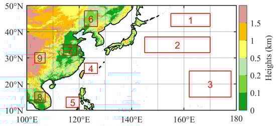
Figure 1.
Terrain heights (color shading, unit: km) of the study area. Nine regions of interest are outlined by red rectangles.

Table 1.
Latitudinal and longitudinal ranges of the nine regions of interest.
The study period covers the whole 3 years from 2017 to 2019. During the 3 years, 85 typhoons formed over the WNP. The impacts of typhoons on the cloud-top-phase climatology are not assessed in this study. The boreal summer (winter) is defined as June, July, and August (December, January, and February).
2.2. Data Description
The meteorological variables used in Section 3 are extracted from the National Centers for Environmental Prediction (NCEP) reanalysis-1 dataset [40] with a spatial resolution of 2.5° × 2.5° and a temporal resolution of 6 h. The SST fields are obtained from the 1° × 1° weekly National Oceanic and Atmospheric Administration (NOAA) Optimum Interpolation version 2 (OI.V2) SST dataset [41].
The cloud-top phase product is generated from AHI/Himawari-8 infrared brightness temperature and cloud mask data based on the retrieval algorithm developed by [42]. This cloud-top phase determination algorithm consists of two water-phase tests, two ice-phase tests, an uncertain-phase test, a cold-cloud test, a cirrus test, and an ice-cloud-edge test. The latter three tests are newly added, in contrast to the Moderate Resolution Imaging Spectroradiometer Level-2 cloud product (MOD06) infrared algorithm of Collection-6 version. Besides, the AHI cloud-top phase algorithm decision tree uses a “water-phase-first” logic [42], which is different from that of Collection-6 MOD06 infrared algorithm.
There are three possible phase classifications in the cloud-top phase product, i.e., water, ice, and uncertain. When coupled with CTT, the water phase can be further refined into being either warm water or supercooled water, depending on whether the CTT is above 0 °C or not. The AHI CTT is derived using the cloud-height retrieval algorithm proposed by [43], with NCEP Global Forecast System analysis data as input.
Evaluated using Cloud–Aerosol Lidar with Orthogonal Polarization (CALIOP) products over a 4-month period from March to June of 2017, the AHI cloud-top determinations give hit rates of 80.20% and 86.51% for CALIOP water and randomly-oriented-ice cloud tops, respectively [42]. Compared to the Collection-6 MOD06 infrared algorithm, the AHI cloud-top-phase algorithm significantly reduces the number of unreasonable ice-phase pixels over oceans and uncertain-phase pixels over land. It also overcomes the limitations for daytime water-phase identifications over the Indo-China Peninsula and the Mongolian Plateau. Note that the AHI-based cloud-top-phase determination algorithm is not yet perfect. An underestimation of the water-phase frequency is found over sunglint regions and during the twilight period. More details can be found in [42].
The AHI cloud-top-phase and CTT products are originally available at 30-min intervals and at a 2-km spatial resolution at nadir. When examining the spatial distribution of cloud occurrence frequencies, each individual pixel was assigned to a 1°×1° grid and counted.
3. Large-Scale Thermodynamic Environments
The large-scale meteorology is a critical factor in determining cloud properties. Any differences in cloud regimes can be largely explained by the different atmospheric conditions. This section first analyzes the large-scale thermodynamic environments to help understand the spatial and temporal distributions of the cloud-top phase.
Figure 2 shows the 5880-gpm contour lines of seasonally averaged 500-hPa geopotential heights, representing the boundaries of the WPSH system [44], for the boreal summer and winter of 2017–2019. In summer, the intensification and northwestward expansion of the WPSH results in the broad coverage of prevalent downdrafts. In winter, however, the WPSH is restricted to a narrow area south of 20° N. Significant annual differences are also found in the locations and extents of WPSH systems. The summertime (wintertime) WPSH was most intense in 2017 (2019), and weakest in 2018 (2017).
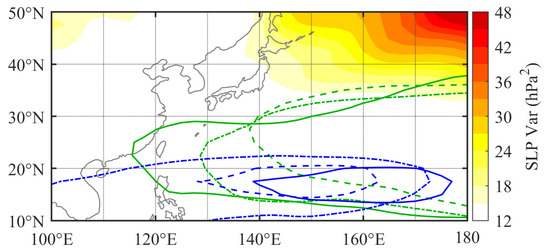
Figure 2.
The sea level pressure (SLP) filtered variance (color shading, unit: hPa2) of National Centers for Environmental Prediction (NCEP) reanalysis-1 for the 3-year (2017–2019) boreal winter. The green (blue) solid, dashed, and dash-dot curves denote seasonally averaged boundaries of the Western Pacific subtropical high-pressure (WPSH) systems in the summer (winter) of 2017, 2018, and 2019, respectively.
Figure 2 also illustrates the density of WNP winter storm tracks. There have been two basic approaches to diagnosing storm tracks. The first one identifies the extratropical cyclones, tracks their positions, and obtains composite analysis for their distributions, while the second one computes Eulerian statistics to describe the storm tracks. This study employs the second approach, identifying storm tracks by the medium-pass filtered variance of sea level pressure (SLP) field [45]. The coefficients for the 2–6-day bandpass filter are provided by Blackmon [46]. Results show a high-density area of WNP winter storm tracks located north of 35° N. By contrast, the density of WNP storm tracks in summer decreases significantly, with SLP filtered variance being lower than 18 hPa2 over the whole WNP ocean (figures omitted).
Differences of lower-tropospheric moisture conditions and near-surface wind distributions over the WNP are found between the summer and winter (Figure 3). In summer, the seasonally averaged relative humidity at 925 hPa is lower than 80% over the whole study area, except for South China and the high-latitude WNP. However, in winter, the 925-hPa relative humidity is greater than 80% everywhere over the ocean. Meanwhile, over land, a moist tongue intrudes along Vietnam’s coastline into the Sichuan Basin. The near-surface sea wind in summer is more meridional over the open seas, accompanied by a weaker south–north SST gradient than that in winter. The near-surface wind field is affected by the East Asian Monsoon [47].
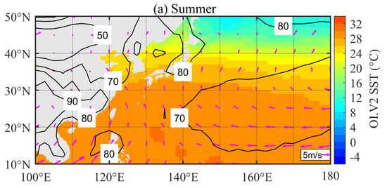
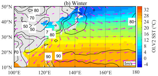
Figure 3.
Seasonally averaged National Oceanic and Atmospheric Administration (NOAA) Optimum Interpolation version 2 (OI.V2) SST (color shading, unit: °C), near-surface wind (magenta vectors with the scale indicated at the bottom-right corner) and 925-hPa relative humidity field (black contours, unit: %) from the NCEP reanalysis-1 using the 3-year boreal (a) summer and (b) winter data.
4. Cloud-Top-Phase Climatology
4.1. Seasonal Variation
Figure 4 shows the frequency distributions of different AHI-derived cloud-top phases over the WNP during the 3-year boreal summer. The statistics were calculated for each 1° × 1° grid of the study area. High frequencies of any-phase clouds (i.e., the cloud top is either water- or ice-phase) are found over the Indo-China Peninsula, the South China Sea, and the WNP east of Hokkaido. The WPSH, where prevalent downdrafts suppress near-surface water vapor divergences and the cloud-top development [48], has low frequencies of any-phase clouds (see the Supplementary Material for more discussions). The frequency of ice clouds during the summer is very similar to that of any-phase clouds except over the WNP east of Hokkaido. The maximum frequency observed over the Indo-China Peninsula and the South China Sea corresponds to activity in the Intertropical Convergence Zone (ITCZ). The frequency subcenter located over the ocean between 30° N and 40° N, commonly in excess of 45%, is caused by the quasi-stationary Meiyu front which usually occurs along the north-west edge of the WPSH. Compared with ice clouds, relatively a few water clouds are observed during summer, except over the WNP east of Hokkaido. The high frequency of water clouds (sea fogs in fact) there is interpreted as the result of warm air advection by the near-surface southerly winds over an area of cold SST, as shown in Figure 3a. The frequency for summertime supercooled water clouds is very low, both over ocean and land.
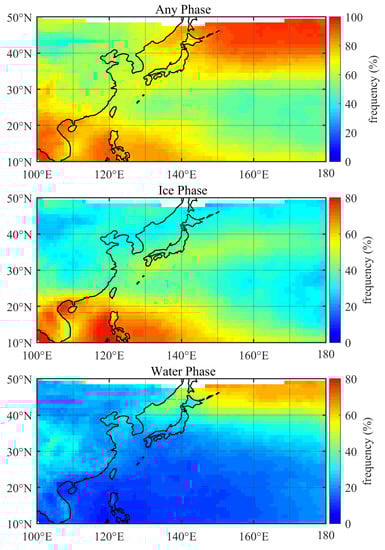
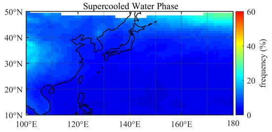
Figure 4.
The 1° × 1° gridded seasonally averaged frequency (unit: %) distributions of cloud-top phases using the 3-year boreal summer data.
Figure 5 presents the frequency distributions of cloud-top phases for the 3-year boreal winter. When changing from summer to winter, the frequency of any-phase clouds in the offshore areas increases significantly. Owing to the southward retreat of the WPSH, the maritime region with a low-frequency (<40%) cloud occurrence is limited to the longitudes between 10° N and 25° N. When focusing on ice clouds, a dramatic drop (from ~40% to ~5%) in frequency is observed between 15° N and 30° N during the winter when compared with summer. High frequencies are found over the ITCZ and within the mid-latitude storm tracks, as shown in Figure 2. Different from ice clouds, water clouds are found to have a dramatically larger spatial extent in winter than summer. Moreover, the winter water-cloud frequency produces a strong maritime–terrestrial discontinuity, highlighting the effect of the underlying surface type on low-altitude clouds. Large frequencies of water clouds are found over the Sichuan Basin as well as over coastal oceans from Hainan to Kyushu. The moist tongue and calm winds over the Sichuan Basin (as shown in Figure 3b) create favorable conditions for the frequent foggy weather in winter. Over oceans, water clouds in winter are frequent because of the high values of low-troposphere humidity. Especially over China’s offshore waters, when the warm Kuroshio waters encounter cold air masses, the exchange of heat and moisture from the oceans into the atmosphere promotes the formation and persistence of low clouds. This study suggests that the water-cloud distributions over the WNP are likely controlled by moisture and wind conditions in the lower troposphere. For wintertime supercooled water clouds, they usually occur north of 25° N, with maximum frequency in R1 and R9.
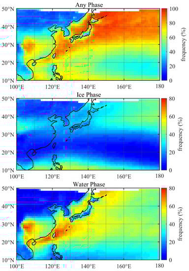
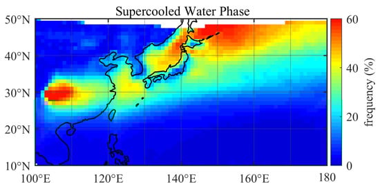
Figure 5.
Same as Figure 4 except using the 3-year boreal winter data.
Figure 6 illustrates the monthly variations in the frequencies of AHI-derived ice and water phases. Results are shown separately for the nine regions of interest, given the large regional variability of cloud-top-phase distributions. Eight of the nine regions have a high frequency of ice clouds in summer. The highest frequencies of ice clouds are in June for the mid-latitude ocean (R2 and R4) and the Yangtze-Huai Plain (R7), in July for the tropics (R5 and R8) and the Sichuan Basin (R9), and in August for the subtropical ocean (R3) and the Manchurian Plain (R6). Over the WNP east of Hokkaido (R1), ice clouds display little seasonality in frequency. Compared with ice clouds, water clouds at low and mid-latitudes are less frequent during boreal summer. The water clouds in R1 and R6 behave differently, with an occurrence frequency peak in summer. In terms of monthly variations in water-cloud frequencies, the low- and mid-latitude maritime regions have only a single peak appearing in the three winter months. Over land, by contrast, the maximum of water cloud frequencies appears in October and November for R9 and in November and January for R8. As a special type of water cloud, supercooled (i.e., CTT < 0 °C) water clouds display similar monthly variations in occurrence frequency. The only exception is over R1, with maximum (minimum) values appearing in February (July).

Figure 6.
Monthly variations in the spatial and monthly averaged frequencies (unit: %) of different cloud-top phases over five maritime regions (left panels) and four continental regions (right panels).
Figure 7 and Figure 8 further present the probabilities of cloud-top phases, divided into 5 °C CTT bins, for the boreal summer and winter, respectively. In summer, convection is active and deep. All nine regions of interest follow the trend that the lowest CTT of ice clouds decreases as the near-surface air temperature increases (Figure 7). The seasonal mean near-surface air temperature is 11.7 °C in the WNP east of Hokkaido (R1). As a result, cloud tops may reach −57 °C. By contrast, cloud tops in the tropics and sub-tropics (R3, R4, R5, R7, and R8) can reach as high as the altitude where the temperature is −75 °C, while the near-surface air temperature is >25 °C. The highest CTT of ice clouds also changes with latitude and near-surface temperature. Ice clouds with CTTs higher than −15 °C can be observed in R1. However, ice cloud tops with temperatures higher than −30 °C are rare in the tropics (R3, R5, and R8). Next, we look at the supercooled water clouds. Among the nine regions, the WNP east of Hokkaido (R1) has the highest frequency of supercooled water clouds (15.0%), followed by the Sichuan Basin (R9, 14.4%). R9 also has the largest fraction (49.1%) of supercooled water clouds out of all (warm plus supercooled) water clouds (Table 2). The fractions of supercooled water clouds are lower over the five maritime regions (<30%, R1–R5) than over the four continental regions (>38%, R6–R9).
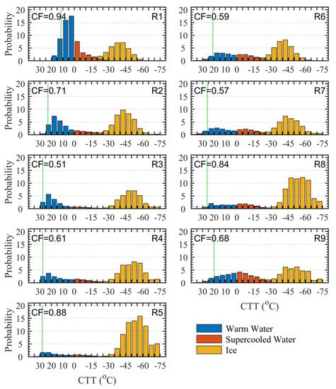
Figure 7.
Probability (unit: %) distributions of cloud-top phases, divided into 5 °C intervals of cloud-top temperature (CTT), for the nine regions of interest in the 3-year boreal summer. The frequency of total cloud occurrence (CF), which is the sum of all CTT bins of the probability, is given in the upper-left corner of each panel. Green vertical lines indicate the seasonal mean near-surface air temperature.
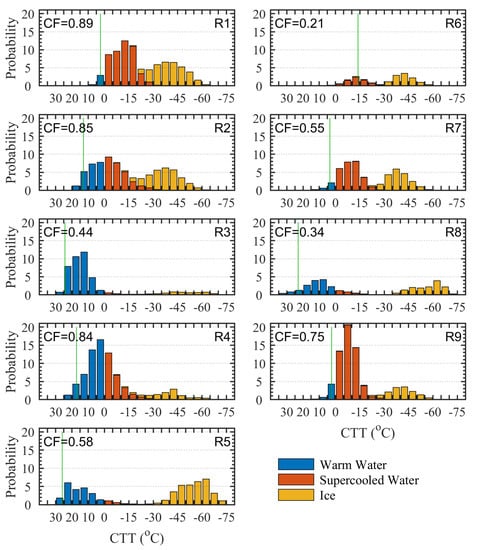
Figure 8.
Same as Figure 7 except for the 3-year boreal winter.
Table 2.
Seasonal mean near-surface air temperatures (Tsfc), total frequencies of supercooled water clouds (SWC Freq.), and fractions of supercooled water clouds out of all water clouds (SWC Frac.) for the nine regions of interest in the 3-year boreal summer and winter.
The ice-cloud trends found in summer still hold in winter (Figure 8), although the frequency of ice clouds drops dramatically. When changing from summer to winter, the frequencies of supercooled water clouds all increase. The most significant growth occurs in R1 and R9, from ~15% in summer to ~50.0% in winter (Table 2). Interestingly, the fraction of supercooled water clouds out of all water clouds during winter seems to be modulated by the near-surface air temperature. If the near-surface temperature is lower than 5 °C (for instance, in R1, R6, R7, and R9), the fraction of supercooled water clouds is in excess of 90%. The largest fractions are observed in R6 and R1, with values of 97.5% and 93.8%, respectively.
4.2. Diurnal Variation
The diurnal variations in the frequencies of different cloud-top phases are examined at the local solar time (LST) for both the summer and the winter. Figure 9 shows the LSTs when the frequencies of AHI-derived cloud-top phases reach their peaks during the summer. On average, ice clouds are prevalent in the late afternoon, ~1800 LST over the land and tropical ocean and 1200–1400 LST over the mid-latitude ocean. The LSTs when the frequency of water clouds is largest are regionally dependent, e.g., at night over the tropical ocean, in the early morning over the subtropical and extratropical ocean, and at noon over the land. The maximum frequencies of any-phase clouds are found in the late afternoon and midnight over most parts of the tropical and subtropical regions. South China, including the Sichuan Basin, has any-phase cloud frequency peaks occurring in the late morning, which agrees well with previous results reported by [37]. Over the high-latitude ocean, any-phase clouds are prevalent in the early morning.

Figure 9.
Local solar times (unit: hour) when the frequencies of different cloud-top phases reach their peak values using the 3-year boreal summer data.
During the winter, water dominates the cloud-top-phase observations. As a result, the maximum frequencies of any-phase clouds and water clouds consistently appear between early morning and noon, regardless of whether the underlying surface is ocean or land (Figure 10). The exceptions are located over the Huai River Basin (around 115° E, 35° N) and Sichuan Basin, where water-phase clouds are most prevalent at night. The behavior of ice clouds is complex in the wintertime. It is hard to conclude when ice clouds are most observed.
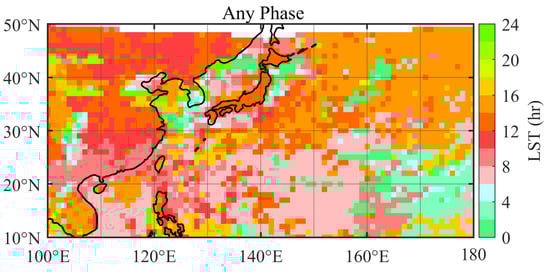
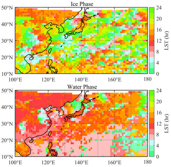
Figure 10.
Same as Figure 9 except using the 3-year boreal winter data.
Figure 11 and Figure 12 provide the diurnal variations in the frequencies of ice, water, and supercooled water phases over the nine regions of interest. The diurnal variations are significant for ice phase over R8 during summer and water phase over R6 during winter. The small amplitudes over the ocean are possibly due to the large heat capacity of water. Note that the diurnal variations for water clouds always have shallow troughs appearing around 0700 and 1700 LST. This feature is caused by the artifacts of the AHI cloud mask algorithm, as mentioned in Section 2.2.
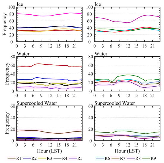
Figure 11.
Diurnal variations in the frequencies (unit: %) of different cloud-top phases over five maritime regions (left panels) and four continental regions (right panels) in the 3-year boreal summer.
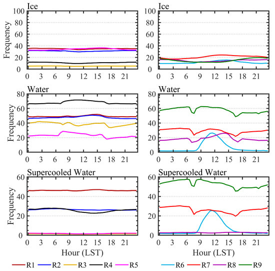
Figure 12.
Same as Figure 11 except for the 3-year boreal winter.
In summer, the diurnal variation in ice cloud frequency over the Sichuan Basin (R9) is weak and has a midnight peak, which is different from the other three continental regions (Figure 11). This feature is linked to the summer nocturnal precipitation in the Sichuan Basin, which is caused by the combined effects of topography, moist air mass transport, and radiative cooling [49]. For summer water clouds over land, a semi-diurnal cycle is found during the daytime, with peaks occurring at noon, reflecting the development of summer mesoscale convection. Zhuge and Zou [50] revealed that local convection in summer often starts with water-phase cloud-top cumulus formed in the morning and glaciated around noon, culminating in a mesoscale convective system mostly observed in the late afternoon. The diurnal variations in supercooled water cloud frequencies are weak over both the ocean and land.
In winter, although complicated by anomalous troughs, peaks in the occurrence of continental water clouds around sunrise can be inferred (Figure 12). This feature is linked to radiation fog, which tends to occur inland during the winter. It often forms during the night due to near-surface water vapor condensation caused by radiative cooling and dissipates after sunrise as the surface temperature increases [51]. However, over the Manchurian Plain (R6), the wintertime water clouds have a peak of occurrence frequencies at noon. Over the tropical continent (R8), wintertime water clouds exhibit a diurnal cycle with its peak in the afternoon. Due to supercooled water dominating water clouds in winter, supercooled-water-cloud frequencies and water-cloud frequencies behave similarly.
Figure 13 and Figure 14 show profiles of the probabilities of AHI-derived ice and water phases at 3-hourly intervals in the 3-year boreal summer and winter, respectively. The CTT used here represents the cloud-top height/pressure because a high correlation is found between the CTT and cloud-top pressure (figures omitted). For clarity, the probability is normalized by the seasonal mean frequency. It is reminded that the water-cloud frequencies estimated during twilight hours are uncertain, as mentioned in Section 2.2. The maritime ice clouds in both summer and winter exhibit little diurnal variation. For continental ice clouds, during both summer and winter, the diurnal variations are represented by a peak value (i.e., occurrence probability) rather than a peak position (i.e., corresponding CTT) in the vertical probability distribution. An exception is over summertime R8, where the peak value remained the same, but the peak position changed by at least 10 °C. Similarly, the probability profiles for the summer maritime water clouds also change the peak values without changing the peak position. However, the profiles for the summer continental water clouds vary greatly, especially during the daytime. At both cold and warm temperatures, the probabilities of summer continental water clouds increase around noon, indicating that an increase in frequency is a result of both the elevated cloud tops and the newly formed boundary-layer clouds. During the winter, large diurnal variations in the probability profiles of water clouds are found in the South China Sea (R5), the Manchurian Plain (R6), and the Indo-China Peninsula (R8). The diurnal variations are mainly represented by the changed frequency of boundary-layer clouds in R5 and R8, while by changed peak values in R6.
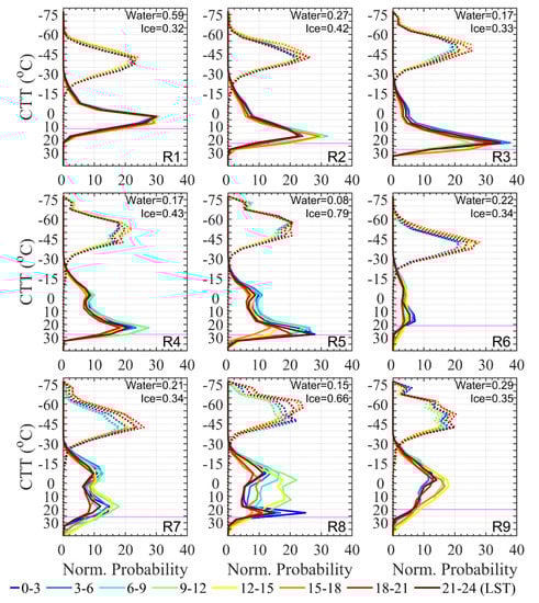
Figure 13.
Normalized probability (unit: %) distributions of water (solid lines) and ice (dotted lines) phases for every 3 h over the nine regions of interest during the 3-year boreal summer with respect to the cloud-top temperature (CTT) calculated at 5 °C intervals. The normalized probability for a certain phase is defined as the actual probability divided by the seasonal mean frequency, indicated in the upper-right corner of each panel. Magenta horizontal lines indicate seasonal mean near-surface air temperatures.
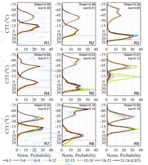
Figure 14.
Same as Figure 13 except for the 3-year boreal winter.
5. Conclusions and Discussions
This study investigates the cloud-top-phase climatology over the WNP based on 3-year AHI retrievals from 2017 to 2019. Seasonal variations in the frequency of various cloud-top phases are examined first. The maritime region with a low frequency of total cloud occurrence coincides roughly with the spatial coverage of the WPSH, in both summer and winter. Ice (water) clouds are more (less) frequent in summer than in winter for the majority of the maritime regions considered. However, the WNP east of Hokkaido in summer has a high frequency of water clouds, caused by warm air advection over an area of cold SST by the near-surface southerly winds. Water cloud distributions in winter over the WNP are likely controlled by the moisture conditions in the lower troposphere. Regarding the continental region, foggy weather frequently occurs in winter over the Sichuan Basin, under the effect of a moist tongue and calm winds. This study also reveals that the CTT range of ice clouds uniformly shifts to lower temperatures as the near-surface air temperature increases, in both summer and winter. The fraction of supercooled water clouds (i.e., CTT < 0 °C) out of all water clouds during winter also seems to be correlated with the near-surface air temperature. During the summer, the fraction of supercooled water clouds is generally lower over maritime regions than over continental regions.
To our knowledge, the diurnal variations in various cloud-top phases have not been studied before. This study shows that continental and maritime ice clouds are mostly observed in the late afternoon. An exception is over the Sichuan Basin, where summer nocturnal precipitation is typical. The frequency peaks of continental water clouds occur at noon in summer but around sunrise in winter. The vertical profiles of AHI-based cloud-top phases at 3-hourly intervals indicate that the increase in the frequency of continental summer water clouds around noon is associated with both the elevated cloud tops and the newly formed boundary-layer clouds.
The inter-hemispheric difference in the cloud-top-phase climatology is highlighted in this study. For example, ice clouds occur more frequently during austral winter than during austral summer over the SO region [15,18]. Over the WNP, however, ice clouds dominate in the boreal summer while water clouds dominate in the boreal winter. Note that Morrison et al. [18] suggested that over the North Pacific (30–60° N, 160° E–140° W), ice clouds are commonly observed in boreal winter. However, based on this investigation, this signal only exists over the high-latitude ocean south of the Aleutian Islands, where the density of mid-latitude cyclone tracks increases in the winter, as demonstrated in Figure 2. Besides, it is reported that the spatial distribution of water-cloud populations has a dependence on latitude and SST over the SO [20,23], resulting in a decrease in water-cloud frequency when moving toward the pole [18]. By contrast, high frequency of water clouds is found year-round over the high-latitude WNP east of Hokkaido, due to warm air advection by the near-surface southerly winds over an area of cold SST. For low- and mid-latitude WNP, the seasonal variations in cloud-top phases are also affected by the East Asian Monsoon, WPSH, and ocean currents. Since the North Atlantic is similarly affected by continental margins, the cloud-top-phase climatologies between the SO and the North Atlantic, which are not investigated in this study, may also be different.
It is worth mentioning that optical imagers (including the AHI) observe clouds from the top, resulting in low-level clouds not being “visible” when high-level clouds of different phases are present. If there is an error in the ice cloud statistical distribution, it will certainly affect the water cloud distribution. It does not come as a big surprise that as ice clouds become more frequent in summer, water clouds become less frequent. The uncertainties in the climatology of water clouds deserve further investigation in a follow-on research.
Supplementary Materials
The following are available online at https://www.mdpi.com/article/10.3390/rs13091687/s1, Figure S1: The 1°×1° gridded frequency distributions of any-phase clouds (shading, unit: %) and seasonally averaged boundaries of the WPSH systems (purple solid curves) in the summer of 2017, 2018, and 2019, respectively, Figure S2: Same as Figure S1, except for winter.
Author Contributions
Conceptualization, X.Z. (Xiaoyong Zhuge); methodology, X.Z. (Xiaoyong Zhuge); software, X.Z. (Xiaoyong Zhuge); validation, X.Z. (Xiaoyong Zhuge), X.Z. (Xiaolei Zou), X.L., F.T., B.Y. and L.Y.; formal analysis, X.Z. (Xiaoyong Zhuge); investigation, X.Z. (Xiaoyong Zhuge); resources, X.Z. (Xiaoyong Zhuge); data curation, X.Z. (Xiaolei Zou) and X.L.; Writing—Original draft preparation, X.Z. (Xiaoyong Zhuge); writing—Review and editing, X.Z. (Xiaolei Zou), X.L. and F.T.; visualization, X.L.; supervision, X.Z. (Xiaolei Zou); project administration, X.Z. (Xiaoyong Zhuge) and X.Z. (Xiaolei Zou); funding acquisition, X.Z. (Xiaoyong Zhuge) and X.Z. (Xiaolei Zou). All authors have read and agreed to the published version of the manuscript.
Funding
This research was funded by the National Key Research and Development Programs of China (2018YFC1507302 and 2017YFC1501603), the Basic Research Fund of Chinese Academy of Meteorological Sciences (2020R002, 2021Z002, 2021Y013, and 2021Y014), and the Natural Science Foundation of Jiangsu Province (BK20201505).
Institutional Review Board Statement
Not applicable.
Informed Consent Statement
Not applicable.
Data Availability Statement
Not applicable.
Acknowledgments
The National Institute of Information and Communications Technology, Japan distributes the AHI/Himawari-8 raw data (https://sc-web.nict.go.jp/himawari/himawari-data-archive.html (accessed on 30 March 2020)). NCEP reanalysis and NOAA OI.V2 SST data are provided by the NOAA/OAR/ESRL PSD, Boulder, Colorado, USA (https://www.esrl.noaa.gov/psd/ (accessed on 30 March 2020)).
Conflicts of Interest
The authors declare no conflict of interest.
References
- Bergeron, T. On the physics of clouds and precipitation. In Procès-Verbaux de l’Association de Météorologie; International Union of Geodesy and Geophysics: Potsdam, Germany, 1935; pp. 156–178. [Google Scholar]
- Korolev, A.; McFarquhar, G.; Field, P.R.; Franklin, C.; Lawson, P.; Wang, Z.; Williams, E.; Abel, S.J.; Axisa, D.; Borrmann, S.; et al. Mixed-phase clouds: Progress and challenges. Meteorol. Monogr. 2017, 58, 5.1–5.50. [Google Scholar] [CrossRef]
- Sun, Z.; Shine, K.P. Studies of the radiative properties of ice and mixed-phase clouds. Q. J. R. Meteorol. Soc. 1994, 120, 111–137. [Google Scholar] [CrossRef]
- Wolters, E.L.A.; Roebeling, R.A.; Feijt, A.J. Evaluation of cloud-phase retrieval methods for SEVIRI on Meteosat-8 using ground-based lidar and cloud radar data. J. Appl. Meteorol. Clim. 2008, 47, 1723–1738. [Google Scholar] [CrossRef]
- Trenberth, K.E.; Fasullo, J.T. Simulation of present-day and twenty-first-century energy budgets of the Southern Oceans. J. Clim. 2010, 23, 440–454. [Google Scholar] [CrossRef]
- Bodas-Salcedo, A.; Hill, P.G.; Furtado, K.; Williams, K.D.; Field, P.R.; Manners, J.C.; Hyder, P.; Kato, S. Large contribution of supercooled liquid clouds to the solar radiation budget of the Southern Ocean. J. Clim. 2016, 29, 4213–4228. [Google Scholar] [CrossRef]
- Wang, Y.; Zhang, D.; Liu, X.; Wang, Z. Distinct contributions of ice nucleation, large-scale environment, and shallow cumulus detrainment to cloud phase partitioning with NCAR CAM5. J. Geophys. Res. Atmos. 2018, 123, 1132–1154. [Google Scholar] [CrossRef]
- Huang, Y.; Siems, S.T.; Manton, M.J.; Thompson, G. An evaluation of WRF simulations of clouds over the Southern Ocean with A-Train observations. Mon. Weather. Rev. 2014, 142, 647–667. [Google Scholar] [CrossRef]
- Huang, Y.; Franklin, C.N.; Siems, S.T.; Manton, M.J.; Chubb, T.; Lock, A.; Alexander, S.; Klekociuk, A. Evaluation of boundary-layer cloud forecasts over the Southern Ocean in a limited-area numerical weather prediction system using in situ, space-borne and ground-based observations. Q. J. R. Meteorol. Soc. 2015, 141, 2259–2276. [Google Scholar] [CrossRef]
- Naud, C.M.; Booth, J.F.; Del Genio, A.D. Evaluation of ERA-Interim and MERRA cloudiness in the Southern Ocean. J. Clim. 2014, 27, 2109–2124. [Google Scholar] [CrossRef]
- Bodas-Salcedo, A.; Williams, K.D.; Field, P.; Lock, A. The surface downwelling solar radiation surplus over the Southern Ocean in the Met Office model: The role of midlatitude cyclone clouds. J. Clim. 2012, 25, 7467–7486. [Google Scholar] [CrossRef]
- Bodas-Salcedo, A.; Williams, K.D.; Ringer, M.A.; Beau, I.; Cole, J.; Dufresne, J.L.; Koshiro, T.; Stevens, B.; Wang, Z.; Yokohata, T. Origins of the solar radiation biases over the Southern Ocean in CFMIP2 models. J. Clim. 2014, 27, 41–56. [Google Scholar] [CrossRef]
- Franklin, C.N.; Sun, Z.; Bi, D.; Dix, M.; Yan, H.; Bodas-Salcedo, A. Evaluation of clouds in ACCESS using the satellite simulator package COSP: Global, seasonal and regional cloud properties. J. Geophys. Res. Atmos. 2013, 118, 732–748. [Google Scholar] [CrossRef]
- Stephens, G.L.; Vane, D.G.; Boain, R.J.; Mace, G.G.; Sassen, K.; Wang, Z.; CloudSat Science Team. The CloudSat mission and the A-Train: A new dimension of space-based observations of clouds and precipitation. Bull. Am. Meteorol. Soc. 2002, 83, 1771–1790. [Google Scholar] [CrossRef]
- Huang, Y.; Siems, S.T.; Manton, M.J.; Protat, A.; Delanoë, J. A study on the low-altitude clouds over the Southern Ocean using the DARDAR-MASK. J. Geophy. Res. 2012, 117, D18204. [Google Scholar] [CrossRef]
- Williams, K.D.; Bodas-Salcedo, A.; Déqué, M.; Fermepin, S.; Medeiros, B.; Watanabè, M.; Jakob, C.; Klein, S.; Senior, C.A.; Williamson, D.L. The Transpose-AMIP II Experiment and its application to the understanding of Southern Ocean cloud biases in climate models. J. Clim. 2013, 26, 3258–3274. [Google Scholar] [CrossRef]
- Hu, Y.; Rodier, S.; Xu, K.; Sun, W.; Huang, J.; Lin, B.; Zhai, P.; Josset, D. Occurrence, liquid water content, and fraction of supercooled water clouds from combined CALIOP/IIR/MODIS measurements. J. Geophys. Res. Atmos. 2010, 115, D00H34. [Google Scholar] [CrossRef]
- Morrison, A.E.; Siems, S.T.; Manton, M.J. A cloud-top phase climatology of Southern Ocean clouds. J. Clim. 2011, 24, 2405–2418. [Google Scholar] [CrossRef]
- Huang, Y.; Siems, S.T.; Manton, M.J.; Hande, L.B.; Haynes, J.M. The Structure of low-altitude clouds over the Southern Ocean as seen by CloudSat. J. Clim. 2012, 25, 2535–2546. [Google Scholar] [CrossRef]
- Huang, Y.; Siems, S.T.; Manton, M.J.; Rosenfeld, D.; Marchand, R.; McFarquhar, G.M.; Protat, A. What is the role of sea surface temperature in modulating cloud and precipitation properties over the southern ocean? J. Clim. 2016, 29, 7453–7476. [Google Scholar] [CrossRef]
- Naud, C.M.; Posselt, D.J.; van den Heever, S.C. Observational analysis of cloud and precipitation in midlatitude cyclones: Northern versus Southern Hemisphere warm fronts. J. Clim. 2012, 25, 5135–5151. [Google Scholar] [CrossRef]
- Mace, G.G. Cloud properties and radiative forcing over the maritime storm tracks of the Southern Ocean and North Atlantic derived from A-Train. J. Geophys. Res. 2010, 115, D10201. [Google Scholar] [CrossRef]
- Naud, C.M.; Del Genio, A.D.; Bauer, M. Observational constraints on the cloud thermodynamic phase in midlatitude storms. J. Clim. 2006, 19, 5273–5288. [Google Scholar] [CrossRef]
- Rienecker, M.M.; Suarez, M.J.; Gelaro, R.; Todling, R.; Bacmeister, J.; Liu, E.; Bosilovich, M.G.; Schubert, S.D.; Takacs, L.; Kim, G.K.; et al. MERRA: NASA’s Modern-Era Retrospective Analysis for Research and Applications. J. Clim. 2011, 24, 3624–3648. [Google Scholar] [CrossRef]
- Huang, J.; Minnis, P.; Chen, B.; Huang, Z.; Liu, Z.; Zhao, Q.; Yi, Y.; Ayers, J. Long-range transport and vertical structure of Asian dust from CALIPSO and surface measurements during PACDEX. J. Geophys. Res. Atmos. 2008, 113, D23212. [Google Scholar] [CrossRef]
- Yu, H.; Remer, L.A.; Chin, M.; Bian, H.; Tan, Q.; Yuan, T.; Zhang, Y. Aerosols from overseas rival domestic emissions over North America. Science 2012, 337, 566–569. [Google Scholar] [CrossRef] [PubMed]
- Hu, Z.; Zhao, C.; Huang, J.; Leung, L.R.; Qian, Y.; Yu, H.; Huang, L.; Kalashnikova, O.V. Trans-Pacific transport and evolution of aerosols: Evaluation of quasi-global WRF-Chem simulation with multiple observations. Geosci. Model Dev. 2016, 9, 1725–1746. [Google Scholar] [CrossRef]
- Coopman, Q.; Riedi, J.; Finch, D.P.; Garrett, T.J. Evidence for changes in arctic cloud phase due to long-range pollution transport. Geophys. Res. Lett. 2018, 45, 10709–10718. [Google Scholar] [CrossRef]
- Jin, Q.; Grandey, B.S.; Rothenberg, D.; Avramov, A.; Wang, C. Impacts on cloud radiative effects induced by coexisting aerosols converted from international shipping and maritime DMS emissions. Atmos. Chem. Phys. 2018, 18, 16793–16808. [Google Scholar] [CrossRef]
- Li, J.; Jian, B.; Huang, J.; Hu, Y.; Zhao, C.; Kawamoto, K.; Liao, S.; Wu, M. Long-term variation of cloud droplet number concentrations from space-based lidar. Remote Sens. Environ. 2018, 213, 144–161. [Google Scholar] [CrossRef]
- Kanitz, T.; Seifert, P.; Ansmann, A.; Engelmann, R.; Althausen, D.; Casiccia, C.; Rohwer, E.G. Contrasting the impact of aerosols at northern and southern midlatitudes on heterogeneous ice formation. Geophys. Res. Lett. 2011, 38, L17802. [Google Scholar] [CrossRef]
- Burrows, S.M.; Hoose, C.; Pöschl, U.; Lawrence, M.G. Ice nuclei in marine air: Biogenic particles or dust? Atmos. Chem. Phys. 2013, 13, 245–267. [Google Scholar] [CrossRef]
- Bessho, K.; Date, K.; Hayashi, M.; Ikeda, A.; Imai, T.; Inoue, H.; Kumagai, Y.; Miyakawa, T.; Murata, H.; Ohno, T.; et al. An introduction to Himawari-8/9—Japan’s new-generation geostationary meteorological satellites. J. Meteor. Soc. Jpn. Ser. II 2016, 94, 151–183. [Google Scholar] [CrossRef]
- Li, Y.; Yu, R.; Xu, Y.; Zhang, X. Spatial distribution and seasonal variation of cloud over china based on ISCCP data and surface observations. J. Meteor. Soc. Jpn. Ser. II 2004, 82, 761–773. [Google Scholar] [CrossRef]
- Jin, X.; Wu, T.; Li, L.; Shi, C. Cloudiness characteristics over Southeast Asia from satellite FY-2C and their comparison to three other cloud data sets. J. Geophys. Res. 2009, 114, D17207. [Google Scholar] [CrossRef]
- Yin, J.; Wang, D.; Xu, H.; Zhai, G. An investigation into the three-dimensional cloud structure over East Asia from the CALIPSO-GOCCP Data. Sci. China Earth Sci. 2015, 58, 2236–2248. [Google Scholar] [CrossRef]
- Chen, D.; Guo, J.; Wang, H.; Li, J.; Min, M.; Zhao, W.; Yao, D. The cloud top distribution and diurnal variation of clouds over East Asia: Preliminary results from Advanced Himawari Imager. J. Geophys. Res. Atmos. 2018, 123, 3724–3739. [Google Scholar] [CrossRef]
- Yang, S.; Zou, X. Lapse rate characteristics in ice clouds inferred from GPS RO and CloudSat observations. Atmos. Res. 2017, 197, 105–112. [Google Scholar] [CrossRef]
- McCoy, D.T.; Hartmann, D.L.; Zelinka, M.D.; Ceppi, P.; Grosvenor, D.P. Mixed-phase cloud physics and Southern Ocean cloud feedback in climate models. J. Geophys. Res. Atmos. 2015, 120, 9539–9554. [Google Scholar] [CrossRef]
- Kalnay, E.; Kanamitsu, M.; Kistler, R.; Collins, W.; Deaven, D.; Gandin, L.; Iredell, M.; Saha, S.; White, G.; Woollen, J.; et al. The NCEP/NCAR 40-year reanalysis project. Bull. Am. Meteorol. Soc. 1996, 77, 437–471. [Google Scholar] [CrossRef]
- Reynolds, R.W.; Rayner, N.A.; Smith, T.M.; Stokes, D.C.; Wang, W. An improved in situ and satellite SST analysis for climate. J. Clim. 2002, 15, 1609–1625. [Google Scholar] [CrossRef]
- Zhuge, X.; Zou, X.; Wang, Y. Determining AHI Cloud-Top Phase and Intercomparisons with MODIS Products over North Pacific. IEEE Trans. Geosci. Remote Sens. 2021, 59, 436–448. [Google Scholar] [CrossRef]
- Heidinger, A.K. ABI Cloud Height Algorithm Theoretical Basis Document (ATBD). NOAA NESDIS Center for Satellite Applications and Research (STAR), Ver. 3.0, Released 06/11/2013. Available online: http://www.star.nesdis.noaa.gov/goesr/docs/ATBD/Cloud_Height.pdf (accessed on 2 June 2018).
- Tao, S.Y.; Chen, L.X. A review of recent research on the East Asian summer monsoon in China. In Monsoon Meteorology; Chang, C.P., Krishnamurti, T.N., Eds.; Oxford University Press: New York, NY, USA, 1987; pp. 60–92. [Google Scholar]
- Hoskins, B.J.; Hodges, K.I. New perspectives on the Northern Hemisphere winter storm tracks. J. Atmos. Sci. 2002, 59, 1041–1061. [Google Scholar] [CrossRef]
- Blackmon, M.L. A climatological spectral study of the 500 mb geopotential height of the Northern Hemisphere. J. Atmos. Sci. 1976, 33, 1607–1623. [Google Scholar] [CrossRef]
- Xu, M.; Chang, C.P.; Fu, C.; Qi, Y.; Robock, A.; Robinson, D.; Zhang, H.M. Steady decline of east Asian monsoon winds, 1969–2000: Evidence from direct ground measurements of wind speed. J. Geophys. Res. Atmos. 2006, 111, D24111. [Google Scholar] [CrossRef]
- Feng, S.; Liu, Q.; Fu, Y.-F. Cloud variations under subtropical high conditions. Adv. Atmos. Sci. 2011, 28, 623–635. [Google Scholar] [CrossRef]
- Jin, X.; Wu, T.; Li, L. The quasi-stationary feature of nocturnal precipitation in the Sichuan Basin and the role of the Tibetan Plateau. Clim. Dyn. 2013, 41, 977–994. [Google Scholar] [CrossRef]
- Zhuge, X.; Zou, X. Summertime convective initiation nowcasting over southeastern China based on Advanced Himawari Imager observations. J. Meteor. Soc. Jpn. Ser. II 2018, 96, 337–353. [Google Scholar] [CrossRef]
- Niu, S.J.; Lu, C.S.; Yu, H.Y.; Zhao, L.J.; Lv, J.J. Fog research in China: An overview. Adv. Atmos. Sci. 2010, 27, 639–662. [Google Scholar] [CrossRef]


Publisher’s Note: MDPI stays neutral with regard to jurisdictional claims in published maps and institutional affiliations. |
© 2021 by the authors. Licensee MDPI, Basel, Switzerland. This article is an open access article distributed under the terms and conditions of the Creative Commons Attribution (CC BY) license (https://creativecommons.org/licenses/by/4.0/).