Fengyun-3D/MERSI-II Cloud Thermodynamic Phase Determination Using a Machine-Learning Approach

Abstract

Global cloud thermodynamic phase (CP) is normally derived from polar-orbiting satellite imaging data with high spatial resolution. However, constraining conditions and empirical thresholds used in the MODIS (Moderate Resolution Imaging Spectroradiometer) CP algorithm are closely associated with spectral properties of the MODIS infrared (IR) spectral bands, with obvious deviations and incompatibility induced when the algorithm is applied to data from other similar space-based sensors. To reduce the algorithm dependence on spectral properties and empirical thresholds for CP retrieval, a machine learning (ML)-based methodology was developed for retrieving CP data from China’s new-generation polar-orbiting satellite, FY-3D/MERSI-II (Fengyun-3D/Moderate Resolution Spectral Imager-II). Five machine learning algorithms were used, namely, k-nearest-neighbor (KNN), support vector machine (SVM), random forest (RF), Stacking and gradient boosting decision tree (GBDT). The RF algorithm gave the best performance. One year of EOS (Earth Observation System) MODIS CP products (July 2018 to June 2019) were used as reference labels to train the relationship between MODIS CP (MYD06 IR) and six IR bands of MERSI-II. CALIOP (Cloud-Aerosol Lidar with Orthogonal Polarization), MODIS, and FY-3D/MERSI-II CP products were used together for cross-validation. Results indicate strong spatial consistency between ML-based MERSI-II and MODIS CP products. The hit rate (HR) of random forest (RF) CP product could reach 0.85 compared with MYD06 IR CP products. In addition, when compared with the operational FY-3D/MERSI CP product, the RF-based CP product had higher HRs. Using the CALIOP cloud product as an independent reference, the liquid-phase accuracy of the RF CP product was higher than that of operational FY-3D/MERSI-II and MYD06 IR CP products. This study aimed to establish a robust algorithm for deriving FY-3D/MERSI-II CP climate data record (CDR) for research and applications.

1. Introduction

Clouds are the important factors for regulating the global energy exchange and water cycle, reflecting and absorbing incident solar radiation and Earth’s outgoing long-wave radiation [1]. As an important geophysical parameter, the cloud thermodynamic phase (CP) product, derived from space-based imaging sensors such as MODIS (Moderate Resolution Imaging Spectroradiometer), including ice, ‘uncertain’, and liquid-water phases, aids further understanding of Earth’s weather and climate systems on global scales. The CP products derived from measurements of satellite imaging sensors [2,3,4] provide a priori and crucial knowledge on cloud-top height (CTH), cloud optical thickness (COT), and cloud-top effective particle size (CPS).

Various retrieval methods for space-based imaging sensors have been developed in the past 20 years to improve the understanding of the natural characteristics of CP. Five mainstream quantitative algorithms, namely, the two-band thermal infrared (IR) method [5], the three-band IR method [6,7], the effective absorption of optical thickness ratio or β index method [8,9], the visible (VIS) and near infrared (NIR) method [10,11], and a joint method using VIS, NIR, and IR bands [12,13], have been developed for deriving CP from polar-orbiting satellite imaging measurements. An algorithm using three IR bands was also developed for official MODIS CP product [7] (MODIS v. 6), while four IR bands (7.3, 8.5, 11, and 12 μm) are used for constructing the β index in distinguishing between CP types from measurements of GOES-R (Geostationary Operational Environmental Satellite) series [9]. The β index method accounts for the influence of surface emissivity, surface temperature, vertical atmospheric water-vapor distribution, and other factors on cloud effective emissivity. An obvious weakness in the IR CP algorithm is that it is challenging and time-consuming to develop corresponding adjustments on various test thresholds for multiple instruments with different spectral characteristics. Thresholds for a given satellite sensor can cause noticeable deviations and incompatibilities when it is applied directly to other similar space-based sensors [14,15,16].

Fengyun-3D (FY-3D) is the new-generation Chinese polar-orbiting meteorological satellite launched in 2017 [17]. MERSI-II (Moderate Resolution Spectral Imager-II) is an optical imaging instrument aboard FY-3D with IR bands similar to those of Aqua/MODIS but with a higher spatial resolution of 250 m. The operational CP algorithm for FY-3D/MERSI-II employs VIS, NIR, and IR bands and cloud texture features to identify CP [18]. Due to the use of the VIS band, the current operational FY-3D/MERSI-II algorithm is not able to retrieve CP at night, and it has relatively low accuracy in ice-phase identification. This study aims to develop an all-day CP retrieval algorithm for FY-3D/MERSI-II. Spectral differences between FY-3D/MERSI-II and Aqua/MODIS IR bands mean that the MODIS CP algorithm cannot be applied directly to FY-3D/MERSI-II without some tests for threshold adjustments and forward radiative transfer calculations.

Since the MODIS CP product was developed with reliable accuracy and precision by the MODIS science team, it can be used as standard reference for developing CP products from most other similar sensors, for example, used for training the machine learning (ML)-based retrieval model for other sensors. In such a way, consistent CP products from other sensors like MERSI-II can be derived. Various ML techniques have been successfully applied in recent years for retrieving the cloud or aerosol parameters from weather or environmental satellite data; those methods include but are not limited to k-nearest-neighbor (KNN), support vector machine (SVM), random forest (RF), and gradient boosting decision tree (GBDT), and the parameters to be retrieved using ML include the cloud-top height (CTH), precipitation, cloud-base height (CBH), cloud phase (CP) [16,19,20,21], aerosol subtype [22], and surface PM_2.5 (particles of ≤2.5 μm) concentrations [23]. ML methods differ from the traditional physical radiation calculations and manually tuned models, in that they can flexibly and efficiently learn hidden relationships among features of large numbers of samples, and they have strong fitting ability for nonlinear variables without consideration of the effects of sensor spectral features. ML algorithms reduce the cost of establishing CP classification models and the time required for cloud classification. Wang et al. (2020) obtained high-precision cloud detection and CP products by separating land surface types using the RF algorithm, with polar-orbit active remote-sensing data (from the Cloud-Aerosol Lidar with Orthogonal Polarization (CALIOP)) being carefully selected to provide reference labels. However, problems persist, for example, with the overlap between active and passive satellite pixels being relatively small and the influence of satellite observation angles not being fully considered [16].

Spaceborne active sensors, such as CALIOP aboard the CALIPSO (Cloud-Aerosol Lidar and Infrared Pathfinder Satellite Observations) satellite [24] and Cloud Profiling Radar (CPR) aboard CloudSat [25] are commonly used to evaluate the performance of IR CP algorithms designed for passive satellite sensors [16,26]. Although the FY-3D satellite has been operational for almost 4 years, there are still insufficient typical matching points with the CALIPSO satellite for ML training and testing; they always pass over each other in the polar regions.

Therefore, an ML-based CP methodology was developed for FY-3D/MERSI-II using MODIS CP products as label data. To reduce algorithm dependence on spectral response features and the empirical thresholds of physical retrieval methods, one year of Aqua/MODIS CP products (July 2018 to June 2019) were used as reference label data to train the relationship between MODIS IR CP and FY-3D/MERSI-II six IR band radiance measurements. The official CALIOP cloud product (v. 4.2) and MODIS CP product, along with the operational FY-3D/MERSI-II CP product from the National Satellite Meteorological Center of China, were used for independent cross-validation. This ML-based CP algorithm is expected to mitigate deviations caused by differences in instrument spectral responses, as well as aid the development of a consistent global CP climate data record (CDR) through reprocessing the historical FY-3D/MERSI-II measurements.

2. Methodology

2.1. The Optimal Machine-Learning Algorithm

ML techniques provide highly effective solutions to pattern recognition problems [27]. Here, five classical ML algorithms were used to train the prediction model for the FY-3D/MERSI-II CP, and the optimum algorithm for CP retrieval was obtained through comparing the results from five independent ML algorithms. The specific implementation steps were as follows:

• Training parameters were selected. BT data from the six FY-3D/MERSI-II IR bands (bands 20—3.8 μm, 21—4.05 μm, 22—7.2 μm, 23—8.55 μm, 24—10.8 μm, and 25—12.0 μm), Airmass (1/cos (satellite zenith angle)), and CP products from MODIS (MYD06; July 2018 to June 2019) were collocated as original features (training samples). To reduce errors caused by rapid changes in cloud properties, only data from two sensors within 5 min difference were collocated;
• The ratio between training data and validation data was set. Note that for selecting the algorithm, only 1% of samples were randomly selected for training and testing with a ratio of 7:3 to reduce the memory occupation and time consumption;
• The performances of five ML algorithms were compared in training the sample set, namely, KNN [28,29], Stacking [30], RF [31], AdaBoost [32], and GBDT [33]. Adjustment parameters and dynamic ranges of the five algorithms are shown in

  Table 1. Adjustment parameters and dynamic ranges of different ML algorithms.

  Algorithm (Dimension)	Parameters and Range of Variation
  Random forest (5 × 5 × 5 × 5 = 625)	The number of trees in the forest (n_estimators): [100, 200, 300, 400, 500]		maximum depth of the tree(max_depth): [10, 20, 30, 40, 50]		minimum number of samples required to split an internal node (min_samples_split): [2, 4, 6, 8, 10]		minimum number of samples required to be at a leaf node (min_samples_leaf): [1, 3, 5, 7, 9]
  AdaBoost (5 × 10 = 50)	maximum number of estimators (n_estimators): [100, 200, 300, 400, 500]				Learning rate (learning_rate): [0.1, 0.2, 0.3, 0.4, 0.5, 0.6, 0.7, 0.8, 0.9, 1]
  K-nearest-neighbor (5 × 2 = 10)	Number of neighbors to use by default for k neighbors queries(n_neighbors): [5, 10, 15, 20, 25]				weight function used in prediction (weight S): ‘uniform’ or ‘distance’
  Gradient Boosting Decision Tree (5 × 10 × 5 × 5 × 5 = 6250)	maximum number of estimators (n_estimators): [100, 200, 300, 400, 500]	Learning rate (learning_rate): [0.1, 0.2, 0.3, 0.4, 0.5, 0.6, 0.7, 0.8, 0.9, 1]		maximum depth of the tree (max_depth): [10, 20, 30, 40, 50]		minimum number of samples required to split an internal node (min_samples_split): [2, 4, 6, 8, 10]		minimum number of samples required to be at a leaf node (min_samples_leaf): [1, 3, 5, 7, 9]
  Stacking	Integration of the above four optimal algorithms

  [19,34,35]. Through these comparisons, the GridSearchCV module in Sklearn, with relatively high accuracy and the shortest running time, was selected to adjust the parameters automatically and iteratively (

  Table 2. Performance of CP classification based on five ML algorithms with optimized parameters.

  Algorithm	Parameter	HR	POD	FAR	Time (s)
  RF	n_estimators = 300; max_depth = 30; min_samples_split = 2; min_samples_leaf = 7	0.91	0.91	0.10	101
  GBDT	n_estimators = 400; max_depth = 30; min_samples_split = 2; min_samples_leaf = 7; learning_rate = 0.4	0.91	0.92	0.10	258
  AdaBoost	n_estimators = 400; learning_rate = 0.8	0.88	0.89	0.11	125
  KNN	n_neighbors = 10; weight S = ‘uniform’	0.84	0.88	0.19	179
  Stacking	Integration of the above four optimal algorithms	0.91	0.91	0.10	648

  RF = random forest; GBDT = gradient boosting decision tree; KNN = k-nearest neighbor.

  ).

Three metrics were used to measure model accuracy, including hit rate (HR, optimal = 1), probability of detection (POD, optimal = 1), false-alarm ratio (FAR, optimal = 0), and elapsed time to measure algorithm running memory (Equations (1)–(3)).

HR = (A + D)/(A + B + C + D),

(1)

POD = A/(A + C),

(2)

FAR = B/(A + B),

(3)

where A is the number of liquid-water-phase pixels also identified as such by the ML training model, B is the number of ice-phase pixels identified as liquid-water phase by the ML training model, C is the number of liquid-water-phase pixels classified as ice phase by the ML training model, and D is the number of ice-phase pixels also identified as such by the ML training model. HR represents the ratio of the number of liquid-water-phase pixels and ice-phase pixels correctly identified by the ML training model to the total number of pixels. It signifies the overall inversion accuracy of liquid-water phase and ice-phase pixels. POD represents the ratio of the correct number of liquid-water-phase pixels identified by the ML training model to the total number of liquid-water-phase pixels. Therefore, a higher POD denotes a higher accuracy of liquid-water-phase inversion. FAR represents the ratio of the number of ice-phase pixels which are classified as liquid-water-phase pixels by the ML training model to the total number of liquid-water-phase pixels retrieved from the ML training model. Apparently, it represents the misjudgment rate of liquid-water phase. Of the five independent ML methods, the running time of the RF was the shortest, with both HR and POD scores being at a high level with a relatively low FAR (Table 2). We found that the RF algorithm gave the best performance. Therefore, the RF algorithm was applied in the subsequent model building.

As a classical bagging ensemble classification and regression technique, the RF algorithm can easily run in a parallel computing mode and capture nonlinear or complex relationships between predictor and predictand [31]. This method trains a large number of decision tree predictors and then ages them on average to improve prediction accuracy and reduce overfitting [19]. The debugging of the RF model requires the use of many parameters, including the number of trees in the forest (n_estimators), the maximum depth of the tree (max_depth), the minimum number of samples required to split an internal node (min_samples_split), and the minimum number of samples required to be at a leaf node (min_samples_leaf). It seems like that larger parameters lead to better model precision. However, model overfitting and memory consumption also occur. The final selection of the optimal model parameters depends on the change in out-of-bag (OOB) scores, which can adequately estimate unbiased estimates (deviations) of the regression or classification models. In this study, the model with the shortest running time and highest fitting degree was selected on the basis of the variation trend of OOB for next step retrieval.

2.2. Training Scheme and Model Configuration

The training and validation sets were derived from overlapping data from Aqua/MODIS and FY-3D/MERSI-II for 2 years (July 2018 to June 2020). The orbits of the two satellites do not coincide completely; hence, the orbit prediction method was adopted to overlap the image times of both orbits passing the same region with a time of difference less than 5 min. The different satellites also have spatial and parallax-effect differences [36]. The zenith angles of both the Aqua and the FY-3D satellites were screened in the overlap region of 0°–45° to reduce image deformation. To ensure that the training samples were representative on a global scale, a sample scheme was used to account for the influence of latitude, season, and overpass time (Figure 1). A total of 70,313,100 geo-located pixels were involved, with 49,546,611 being used for validation.

As found in previous studies [19,35,37], an increase in the number of samples may not significantly improve model performance under similar distributions. There were a large number of collocated pixels for FY-3D and Aqua during the June 2018 to July 2019 period; thus, a sensitive analysis was undertaken to determine the optimum number of samples. Totals of 3000, 5000, 10,000, 30,000, 50,000, 100,000, 300,000, or 500,000 pixels of training data were used, with 100,000 pixels being the optimum, above which further increases had no significant effect on model accuracy.

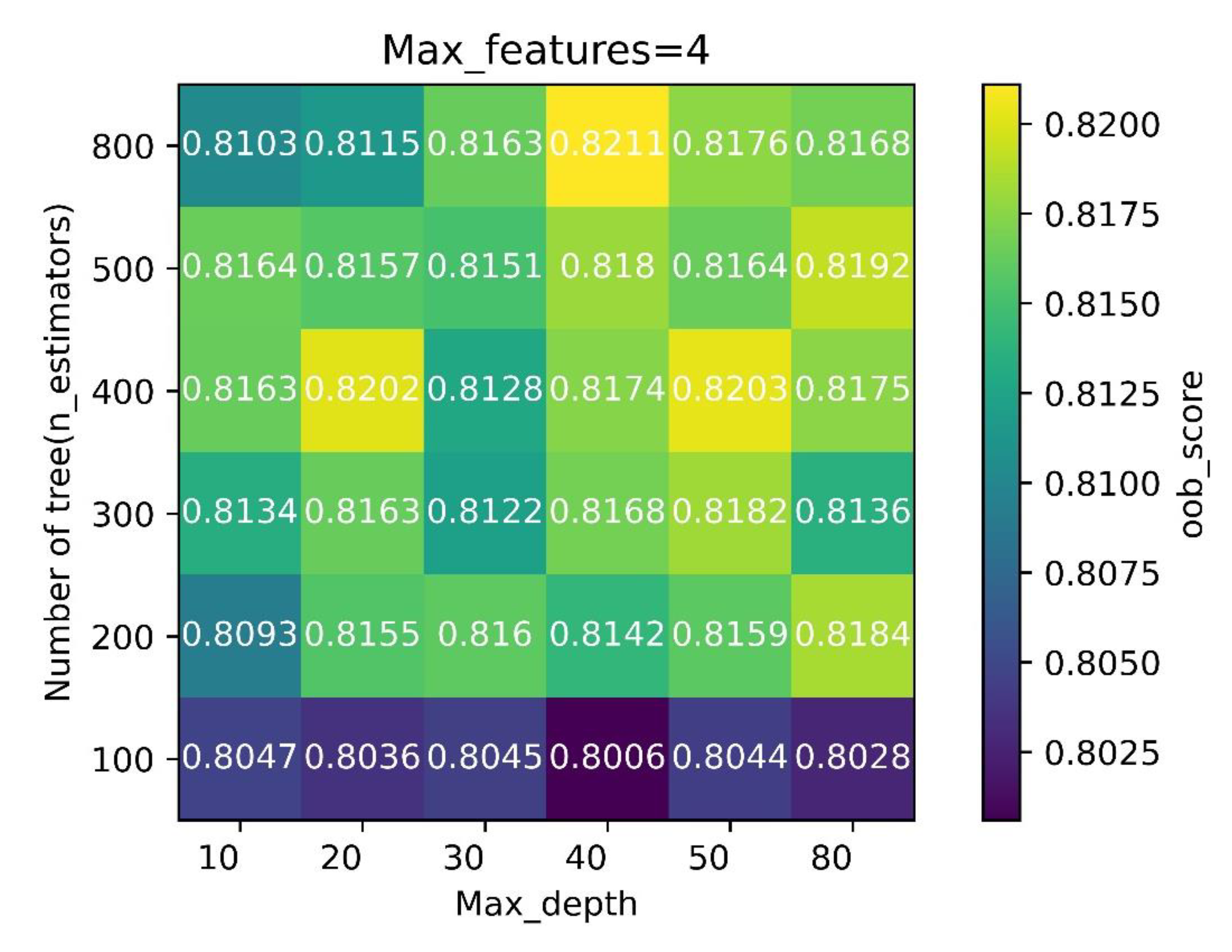
According to RF software package documentation, the empirical default value of random-split predictor variable max_features for the RF classification model is equal to the square root of the total number of predictive variables or features (http://scikit-learn.org/stable/modules/ensemble.html, accessed on 12 April 2021), and this parameter was set on the basis of model input-variable data. Due to the change in the amount of training data, related parameters of the RF model were retrained iteratively. The OOB score represents the fitting result of the unbiased estimation of the RF model; a higher OOB score denotes a better fit of the model. A higher number of trees in the forest (n_estimators) and a greater maximum depth of the trees (max_depth) lead to higher model fitting accuracy and a more complex model. Therefore, it is necessary to find a balance between model accuracy and running time by iterative training.

When n_estimators = 400 and max_depth = 20, the OOB score was higher than other models with similar running times (Figure 2). It had a short running time while maintaining the OOB value. Similarly, the balance of liquid-water and ice phase sample sizes can also significantly affect the accuracy of the final prediction [19,37]. Statistics for the number of liquid-water and ice phase samples during July 2018 to June 2019 indicated a liquid-water-to-ice-phase ratio during the northern mid-latitude summer of 1.56:1, with winter and spring–autumn ratios of 1.02:1 and 1.21:1, respectively. At low and high latitudes, the ratios were 1.35:1 and 0.8:1, respectively. Accordingly, the liquid-water-to-ice-phase ratio was set to the mean of 1.18:1. After iterative training and filtering, the optimal model configuration acquired had the following parameters: n_estimators = 400; max_depth = 20; min_samples_split = 2; min_samples_leaf = 7; max_features = 4; N (number of pixels in training set) = 100,000.

The sensitivity of input variables can be calculated using feature_importances in the RF algorithm, with the sum of importance of all variables being 1. Each input variable has its own physical characteristics and has a close relationship with the cloud phase (

Table 3. The importance scores of predictive variables in the RF model and their corresponding rankings based on the configuration n_estimators= 400, max_depth = 20, min_samples_split = 2, min_samples_leaf = 7, and max_features = 4 for CP classification.

Variable	Importance Score for Variable	Ranking	Physical Characteristics
BTD (8.6–10.8 μm)	0.2015	1	8–10 µm is the weak absorption region of particles.
BTD (10.8–12.0 μm)	0.1080	2	Stronger increases in the absorption of ice particles can be found at 10–11 μm than that at 11–12 μm, while the effect on water particles is the opposite. This allows distinguishing between ice and water particles.
BT (7.2μm)	0.1070	3	The water vapor absorption channel is very sensitive to the amount of water vapor
BTD (3.8–10.8 μm)	0.0891	4	Difference between split–window channel
BTD (4.1–10.8 μm)	0.0800	5	Difference between split–window channel
BT (12.0 μm)	0.0769	6	Total water and sea surface temperature
BTD (7.2–10.8 μm)	0.0618	7	Difference between split–window channel
BT (10.8 μm)	0.0613	8	Split–window channel
BT (8.6 μm)	0.0575	9	Surface temperature, cloud phase, and cirrus cloud detection
BT (3.8 μm)	0.0571	10	Cloud effective particle radius, clouds, and underlying surface temperature
BT (4.1 μm)	0.0508	11	Clouds and underlying surface temperature
Airmass (1/cos(satellite zenith angle))	0.0490	12	Reduces the inversion error caused by the path of light in the atmosphere

). The higher the importance of a variable, the more sensitive it is in the model training. The order of sensitivity of variables and their importance is shown in Table 3.

3. Data

3.1. Reference Pixel Label

The Aqua polar-orbiting satellite was launched on 4 May 2002 at 1:30 p.m. local-time in a sun-synchronous orbit [38], similar to the FY-3D satellite. The MODIS sensor aboard Aqua has 36 spectral bands, covering the spectrum from VIS to IR (0.4–14 μm). The EOS/MODIS Collection-5 CP product and early collections combine 8–11 μm brightness temperature (BT) differences (BTDs) and 11 μm BT to distinguish ice, liquid-water, and mixed-phase clouds through a series of decision trees and thresholds [3]. To further reduce the influence of land surface radiation, the University of Wisconsin-Madison team improved the current CP algorithm from MODIS Collection-6 [3,8,9], providing an additional 1 km resolution CP product for MODIS based on the 7.3, 8.5, 11, and 12 μm bands for constructing the β index and BTD in distinguishing cloud phases through decision trees [9]. The cloud phase is usually classified into three categories: ice, liquid-water, and ‘uncertain’; however, because of the difficulty in distinguishing mixed-phase and uncertain categories in the MODIS Collection-6 CP product, they were merged into one ‘uncertain phase’ category [3]. Here, we conducted training only for certain ice-phase and liquid-water-phase cloud samples (the ‘uncertain’ phase was not considered).

Considering the rapid movement and evolution of clouds, the MODIS Collection-6 CP product (1 km resolution) from July 2018 to June 2019 was carefully geo-located with FY-3D/MERSI-II Level-1B data, within 5 min temporal difference. The Aqua/MODIS Collection-6 CP product was obtained from the US National Aeronautics and Space Administration (NASA) website (https://modis.gsfc.nasa.gov/, accessed on 12 April 2021).

3.2. FY-3D/MERSI-II

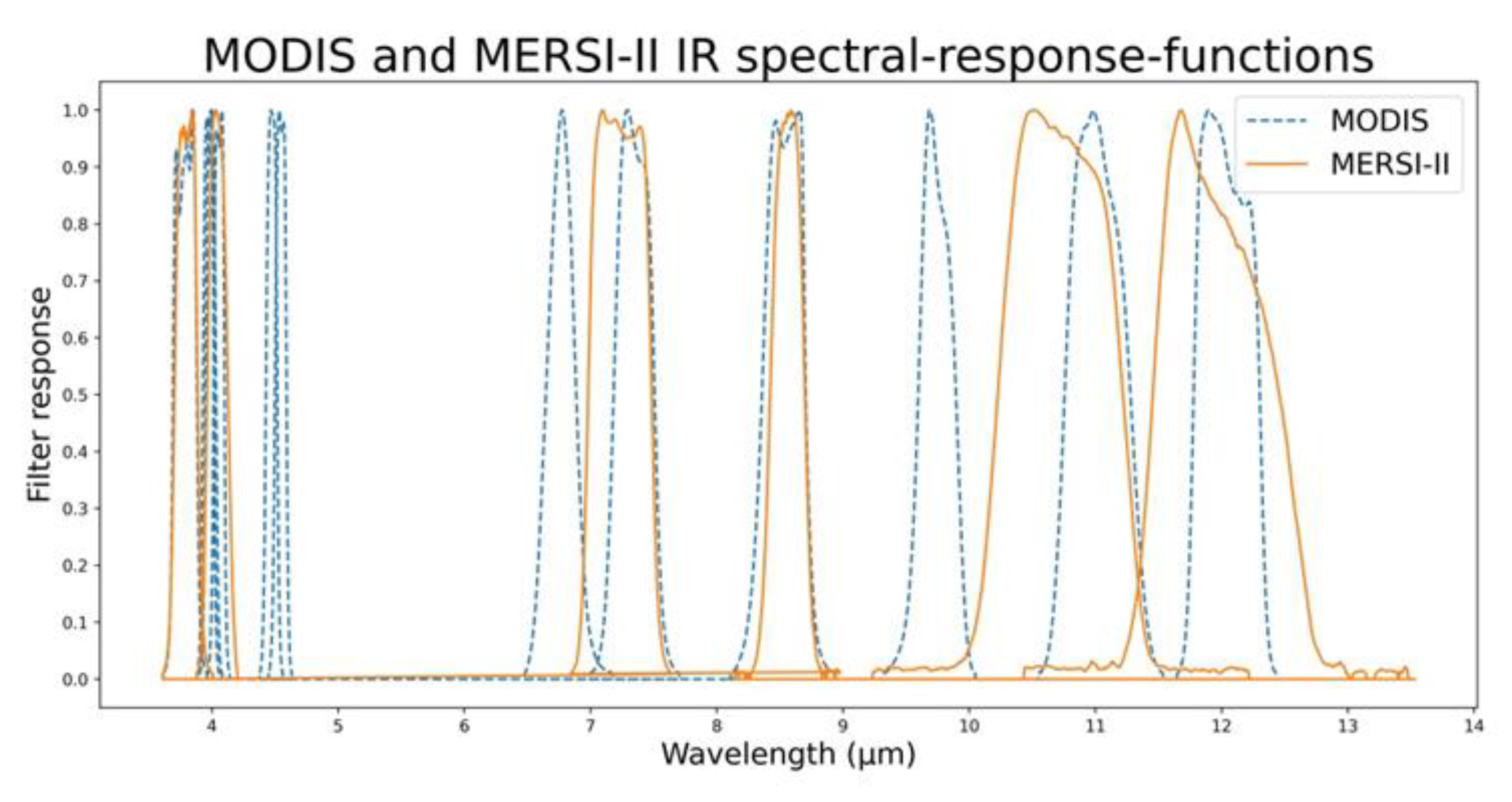
FY-3D/MERSI-II is capable of global observations with two IR split-window bands of 250 m resolution, providing possible high-precision quantitative atmospheric, land, and oceanic products such as cloud, aerosol, water vapor, land surface characteristics, and ocean water color [39]. L1 data were obtained from the Fengyun Satellite Data Service Network (http://satellite.nsmc.org.cn/, accessed on 12 April 2021). Compared with the previous MERSI-I [40], the improved MERSI-II added NIR and IR spectral bands with central wavelengths of 1.38, 3.8, 4.05, 7.2, and 8.55 μm. The original 250 m resolution spectral band of central wavelength 11.25 μm (bandwidth 2.5 μm) was converted to two split-window bands of central wavelengths 10.8 and 12 μm. These IR bands also allow CP determination at night. Moreover, FY-3D/MERSI-II has similar six IR spectral bands of MODIS, which were used for CP training. The bandwidths of some FY-3D/MERSI-II IR bands are slightly wider than those of Aqua/MODIS, along with different central wavelengths (see Figure 3). These differences in sensor spectral features may lead to noticeable deviations in CP retrievals if the MODIS algorithm is directly applied to FY-3D/MERSI-II.

The National Satellite Meteorological Center/China Meteorological Administration (NSMC/CMA) has made an operational CP product based on MERSI-II available since October 2018. This operational CP product is developed using a combination of MERSI-II VIS (0.88–0.68 μm), NIR (1.55–1.64 μm and 3.55–3.93 μm), and two IR (10.3–11.3 μm and 11.5–12.5 μm) spectral bands [18]. Both the spectral and the texture characteristics of VIS, NIR, and IR bands are used to determine CP on a pixel basis with a series of thresholds for classifying liquid-water, ice, or mixed phases. The definition of the mixed phase in the FY-3D/MERSI-II CP product differs from that in the MODIS product, with the former being defined as the mixed-phase state of liquid-water and ice phases. When the reflectivity in the 1.65 and 3.75 μm bands is greater than a given threshold value, the phase is identified as a supercooled water cloud or mixed phase. In spite of both supercooled water and mixed-phase clouds exhibiting a liquid-water phase, they are categorized as ice phase due to their relatively low temperature [41] (<0 °C). For MODIS, water droplets at the top of the cloud layer and fuzzy ice particles that grow within the cloud (and fall through the cloud base) are identified as mixed phase, with mixed-phase and ‘undetermined’ classes being combined to reduce ambiguity [3]. The use of VIS bands in the FY-3D/MERSI-II CP algorithm means it can generate CP product only during daytime. Li et al. (2019) reported that the FY-3D/MERSI-II CP product has biases in ice clouds.

3.3. CALIOP Cloud Products

The CALIPSO satellite was launched in 2006 with CALIOP, a wide-field camera (WFC), and an infrared imaging radiometer (IIR) aboard [42]. CALIOP is the first spaceborne cloud and aerosol lidar with three detection channels (1064 and 532 nm vertical and parallel channels) providing accurate high-resolution vertical profiles of aerosols and clouds globally [43]. The CALIOP cloud classification product includes liquid-water, ice, oriented ice crystals, and ‘unknown’ types. Validation products were derived from the CALIPSO 1-km cloud product (v. 4.20) with CALIOP cloud-top phase information [44]. Since Aqua and CALIPSO are in the ‘Afternoon (A)-train’ constellation, they have the same trajectories and cover the same areas in adjacent time [25]. To reduce the influence of vertically distributed mixed-phase cloud on validation, only single-layer cloud samples detected by CALIOP were used here.

4. Validation and Discussion

4.1. Validation Using Independent MODIS CP Product

Spectral surface emissivity, surface type, and snow and ice coverage are all related to cloud and aerosol retrievals [45,46]; thus, for validation, different surfaces were classified according to latitude and season. Data for July 2019 to June 2020 (Section 3.1) were input into the trained RF model for validation. For subsequent product comparisons, the consistency of product phase states must be ensured. Here liquid water was defined as positive and ice as was defined as negative. Five classical indices were used to evaluate the classification results of liquid and ice phases: POD, FAR, HR, critical success index (CSI, optimal = 1), and Heidke skill score (HSS, optimal = 1). These are defined as follows:

CSI = A/(A + B + C),

(4)

HSS = 2(AD − BC)/[(A + C)(A + D) + (A + B)(B + D)],

(5)

where A is the number of pixels that both MODIS reference CP and the FY-3D/MERSI-II CP retrieved from the ML model (this study) are classified as liquid-water phase, B represents the number of pixels identified as ice phase by MODIS but classified as liquid-water phase by MERSI-II in this study, C is the number of pixels labeled as liquid-water phase by MODIS but classified as ice phase by MERSI-II in this study, and D is the number of pixels that both the MODIS reference CP and the MERSI-II CP of this study classified as ice phase.

A high POD value indicates high accuracy in liquid-water phase identification, while a low FAR value indicates high accuracy in ice-phase identification; the highest CSI index indicates the highest success rate of retrieval model for the liquid-water phase. As can be seen from

Table 4. Statistics of performance metrics of CP classification for different seasons and latitudes.

Classification	POD	FAR	CSI	HR	HSS
Mid-latitude spring and autumn	0.91	0.13	0.76	0.86	0.72
Mid-latitude winter	0.80	0.08	0.74	0.82	0.61
Mid-latitude summer	0.90	0.08	0.84	0.87	0.63
Low latitude all year	0.91	0.13	0.77	0.84	0.68
High latitude all year	0.94	0.11	0.84	0.90	0.8
All year	0.85	0.06	0.80	0.84	0.60

, except for mid-latitude winters, the POD values of all categories were >0.9, FAR values were <0.2, and HR values were >0.8. The four evaluation indices for the mid-latitude summer were all relatively high with the best performance. POD in the mid-latitude winter was only 0.8, but FAR was relatively low. A low liquid-water cloud detection rate led to reduced HR. The influence of snow cover may have contributed to the low detection rate of liquid water in mid-latitude winters when snow cover was not uniform because of the mixed pixel effect, and high snow reflectivity affected accuracy for other surface types near the snow-covered area, which, in turn, influenced the accuracy of classification by the RF model. Wang et al. (2020) found that the MODIS CP product accuracy for snow, ice, and barren surface types is much lower than that of other types, leading to the identification of too many liquid-water phases as ice phases, consistent with the MERSI-II results in this study. The quality of the MODIS CP product resulted in a reduction in liquid-water phase detection capability; performances in mid-latitude spring and autumn and at low latitudes were generally similar, with relatively high POD and high FAR, indicating the classification of too many ice-phase clouds as liquid-water phase. At high latitudes, where there are large areas of ice and snow cover, the total annual POD reached 0.94, and FAR was relatively low, indicating good ML performance, which differs from the results of Wang et al. (2020). This inconsistency may be due to the FY-3D and Aqua satellite orbits generally overlapping at high latitudes, since both training and validation data with small satellite viewing angles at high latitudes are more prevalent than in the mid-latitude winter.

4.2. Comparison of Spatial Distributions

To better understand the reliability of the FY-3D/MERSI-II CP retrieval method based on the ML approach, the trained RF CP product was further compared with the MODIS CP product, as well as the operational FY-3D/MERSI-II CP product. Five images were randomly selected from each region of mid-latitude winter, mid-latitude spring and autumn, mid-latitude summer, low, and high latitudes. In the RF classification process, each pixel was assigned a SCORE: if >0.5, the classification tended toward the liquid-water phase; if <0.5, the classification tended toward the ice phase; if around 0.5, the classification model had no obvious CP classification. Pixels with a score of 0.48–0.52 were defined as being of an ‘uncertain’ phase. For each latitude and season, a total of 15 random images of FY-3D and Aqua with coincident areas were selected for comparison. Overlapping pixels of liquid-water or ice phase in each image were extracted for comparison, and the POD, FAR, CSI, HR, and HSS precision indices were calculated. Results are shown in

Table 5. Statistics for the performance metrics of CP classification when comparing RF CP product and operational FY-3D/MERSI-II CP product, based on images from five time periods representing five categories of season and latitude.

Time	Picture	CP Product	POD	FAR	CSI	HR	HSS
11 October 2020 14:10	Mid-latitude spring and autumn	RF	0.90	0.17	0.76	0.84	0.67
		FY-3D/MERSI-II	0.82	0.17	0.70	0.80	0.60
12 July 2020 12:25	Mid-latitude winter	RF	0.95	0.06	0.95	1.00	0.97
		FY-3D/MERSI-II	0.99	0.06	0.99	1.00	0.99
12 July 2020 9:30	Mid-latitude summer	RF	0.60	0.35	0.45	0.84	0.53
		FY-3D/MERSI-II	1.00	0.60	0.40	0.67	0.38
11 October 2020 15:35	Low latitude	RF	0.90	0.07	0.85	0.90	0.80
		FY-3D/MERSI-II	0.91	0.09	0.79	0.90	0.80
11 October 2020 20:20	High latitude	RF	0.61	0.19	0.54	0.86	0.61
		FY-3D/MERSI-II	0.03	0.11	0.03	0.74	0.04

.

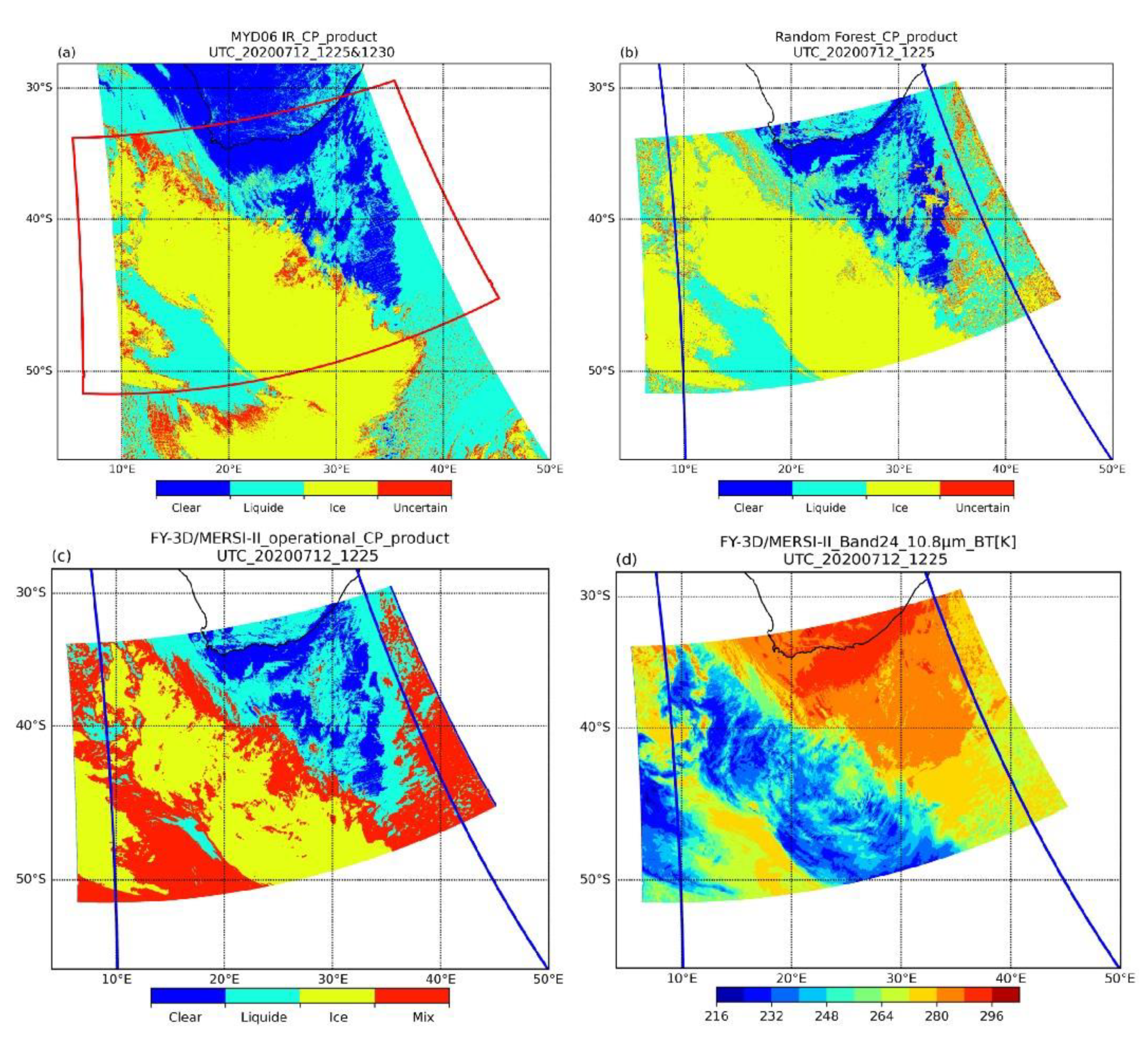
The MODIS, RF FY-3D, and operational FY-3D CP products are compared in Figure 4, Figure 5, Figure 6, Figure 7 and Figure 8 where images highlight the spatial differences in the three products. As the liquid-water phase temperature is higher than that of the ice phase, the FY-3D/MERSI-II band 24 (10.3–11.3 μm) BT could be set as the reference image, whereby bluer colors denote lower temperatures and redder colors denote higher temperatures. Hence, cooler clouds are in blue, while warmer clouds are in red. Figure 4 demonstrates that, in mid-latitude spring and autumn, the RF CP product (Figure 4b) is consistent with the MODIS CP product (Figure 4a). In the area of 60°N 10°W, operational FY-3D/MERSI-II CP product (Figure 4c) identifies most liquid-water phases as ice and mixed phases, as reflected in the BT image (Figure 4d). In the region near 61°N 12°W, the RF CP indicated an ice phase in most liquid-water-phase regions of the MODIS CP product, with the RF product being able to identify fine ice-phase regions. CP retrieval results obtained by the RF algorithm were significantly improved compared with those of the operational FY-3D algorithm (Table 5), with POD increasing from 0.82 to 0.90.

In the mid-latitude winter, RF products and MODIS CP products had strong spatial consistency (Figure 5). In the area 48°S 15°E, many pixels were identified as liquid-water phase by both RF (Figure 5b) and MODIS CP products (Figure 5a). However, for the operational FY-3D/MERSI-II CP product (Figure 5c), these pixels were classified as mixed phase because the definition of mixed phase in the operational FY-3D/MERSI-II CP product differs from the definition of uncertain phase in the MODIS algorithm. Apart from the mixed phase, the mid-latitude winter RF CP product performed comparably with the operational FY-3D CP product (Table 5).

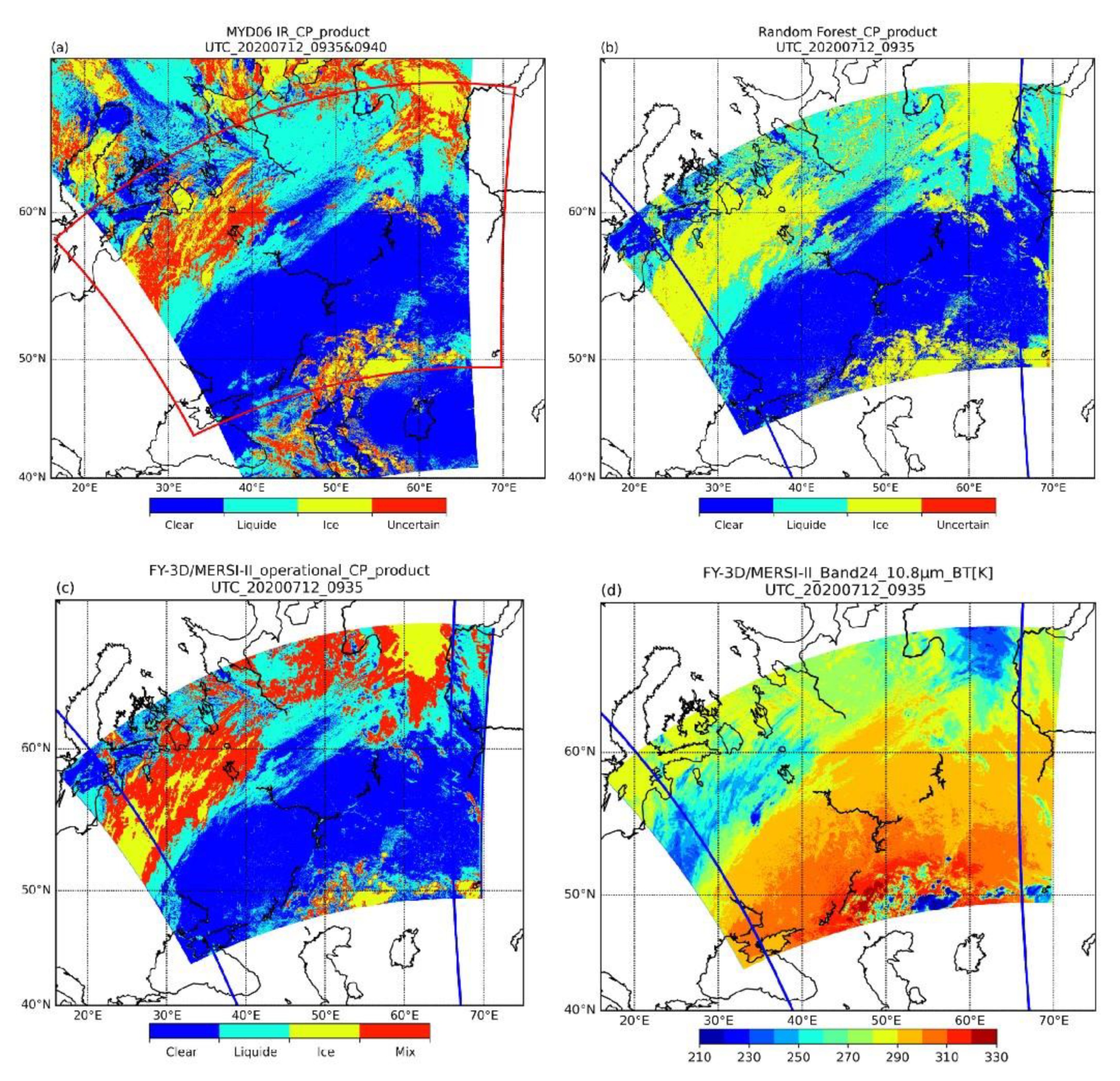
Very few uncertain phases were produced by the RF method in the mid-latitude summer (Figure 6), due mainly to the relatively strict threshold for that phase. More pixels were identified as uncertain or mixed phases for the MODIS (Figure 6a) and operational MERSI-II CP products (Figure 6c). In the area near 65°N 50°E, the operational MERSI-II CP product gave a large number of pixels of mixed phase, whereas, for the MODIS and RF products (Figure 6b), this region was covered mainly by liquid-water and ice phases, respectively. The significant reduction in FAR for the RF CP product represented an improvement in ice-phase detection accuracy (Table 5), and its POD decrease indicated a reduction in liquid-water phase detection capability. The CSI, HR, and HSS of RF CP product all increased significantly while FAR decreased, indicating the improved ice-phase detection capability of the RF CP product associated with an overall increase in detection accuracy.

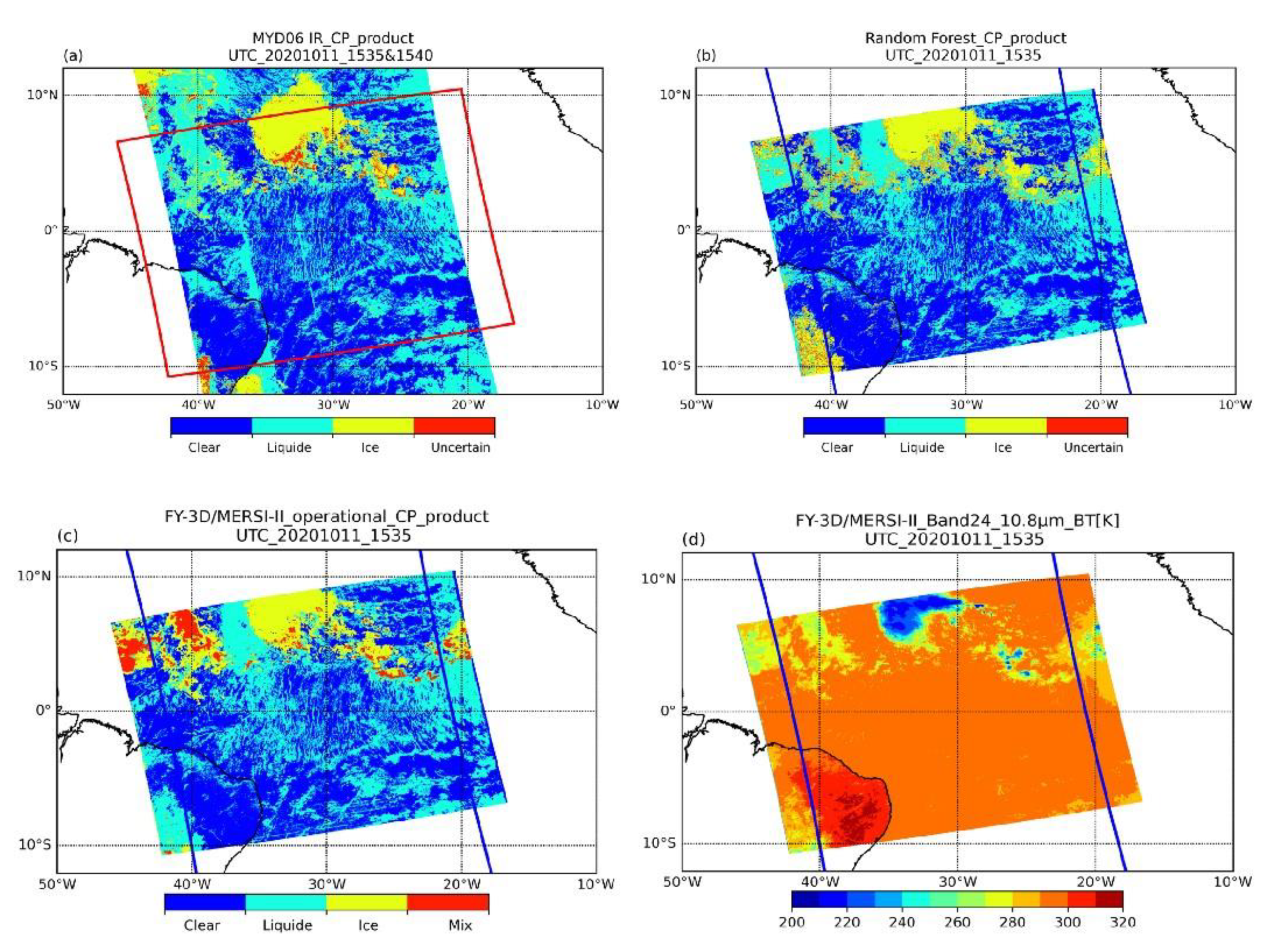
The three products had strong spatial consistency in the low-latitude region (Figure 7), although the cloud detection results of MODIS (Figure 7a) and FY-3D (Figure 7c) were significantly different. In the area near 7°N 40°W, the operational FY-3D/MERSI-II cloud mask product was significantly different from MODIS CP product. Just as in the mid-latitude spring and autumn case (Figure 6), the operational FY-3D/MERSI-II CP product identified ice and mixed phases in areas where the other two products identified a liquid-water phase. With the reduction in FAR, the accuracy of ice-cloud detection for the RF CP product was improved with CSI increasing significantly (Table 5).

The RF CP product obtained from the high latitude was obviously more consistent with MODIS CP product than the FY-3D product (Figure 8). FY-3D CP products (Figure 8c) generally inverted liquid-water phase to ice phase, with almost all liquid-water phases being wrongly identified as ice phases in the operational FY-3D CP product in high-latitude images (Table 5). The RF CP product (Figure 8b) significantly improved liquid-water phase detection capability while ensuring the accuracy of ice phase identification, which also significantly increased CSI, HR, and HSS.

From the above five comparisons, it can be seen that RF-derived CP and MODIS CP were generally consistent. Compared with these two products, too many liquid-water phase pixels were identified as ice phase in the operational FY-3D CP product in almost all cases regardless of season and latitude. The accuracy of the RF CP product in each case was higher than or equal to that of the operational FY-3D CP product, indicating that the consistency between MODIS and RF CP was much better than with the operational FY-3D/MERSI-II product. However, there were two disadvantages with the RF approach: (1) in the process of pixel basis for retrieval, the derived CP image might appear discontinuous, i.e., there are isolated pixels with a cloud phase different from that of neighboring pixels; (2) the determination of the threshold range of the uncertain phase is a problem affecting the size of the uncertain-phase region, with the threshold here being set according to experience, which might have influenced the final results.

4.3. Comparison with Active CALIOP CP Data

When the optical thickness is low, cloud products retrieved from spaceborne active lidar systems (e.g., CALIOP) are often regarded as true values in determining the quality of passively observed cloud products [42]. Here, the MODIS CP, RF, and operational FY-3D/MERSI-II products were further validated using CALIOP cloud-top phase data from the CALIPSO 1 km resolution cloud product. As the liquid-water and ice phases of the MODIS IR CP product were used as reference labels, the quality of the product should be assessed to test the accuracy of the MODIS CP product against ‘true’ liquid-water and ice phase detections. The accuracy of the RF and operational FY-3D CP products should also be assessed relative to the CALIOP CP product. These validations were undertaken as described below.

First MODIS, RF, operational FY-3D/MERSI-II, and CALIPSO/CALIOP cloud products collected within 5 min of each other from July 2019 to June 2020 were collocated, and a dataset of collocated pixels was generated. From this dataset, only pixels identified as liquid-water and ice phase in MODIS CP product were selected and labeled as single-layer clouds in CALIOP (other pixels in the dataset were removed). The numbers of liquid-water and ice phase pixels in MODIS CP, RF, and CALIOP were calculated (

Table 6. CALIOP cloud-top phase cross-validation with MODIS IR, RF, and operational FY-3D/MERSI-II CP products based on season and latitude (the uncertain phase in MODIS and RF products was eliminated, and the mixed and ice phases were merged in the operational FY-3D/MERSI-II product).

CALIOP Phase		MODIS IR Phase		RF Phase		FY-3D Phase
		Liquid	Ice	Liquid	Ice	Liquid	Ice
mid-latitude spring and autumn	Liquid	75.0%	25.0%	88.3%	11.7%	56.1%	43.9%
	Ice	6.6%	93.4%	6.6%	93.4%	5.4%	94.6%
Mid-latitude Winter	Liquid	96.4%	3.6%	87.6%	12.4%	69.8%	30.2%
	Ice	18.7%	81.3%	50.0%	50.0%	7.8%	92.2%
Mid-latitude Summer	Liquid	75.2%	24.9%	77.12%	22.8%	87.6%	12.4%
	Ice	19.4%	80.6%	13.4%	83.6%	18.7%	81.3%
Low latitude	Liquid	65.1%	34.9%	61.9%	38.1%	73.5%	26.5%
	Ice	6.0%	94.0%	12.6%	87.4%	31.0%	69%
High latitude	Liquid	72.1%	27.9%	75.9%	24.1%	16.2%	83.8%
	Ice	5.9%	94.1%	6.3%	93.7%	2.5%	97.5%
	Oriented ice crystal	0	100%	0	100%	0	100.0%
All	Liquid	76.8%	23.2%	78.2%	21.8%	60.6%	39.4%
	Ice	11.3%	88.7%	18.4%	81.6%	13.1%	86.9%
	Oriented ice crystal	0	100%	0	100%	0	100%

Yellow shading represents the correct probability of the CP products.

). For the operational FY-3D/MERSI-II product, the phase corresponding to overlapping pixels included liquid-water, ice, and mixed phases. As the temperature of the mixed phase is below the freezing point (0 °C), it was categorized as ice phase. The accuracies of the MODIS, RF, and operational FY-3D/MERSI-II products were compared and validated against the CALIOP CP benchmark.

The RF and MODIS CP products generally had comparable accuracy (Table 6). In mid-latitude summer and mid-latitude spring and autumn, the RF approach demonstrated slightly better ability in identifying the ice phase. In high latitudes, mid-latitude summer, and mid-latitude spring and autumn, the RF approach detected more liquid-water phases than MODIS. The performance of the RF model in the mid-latitude winter was significantly poorer than that of MODIS, which remains a problem to be addressed. The retrieval accuracy of the operational FY-3D/MERSI-II CP product was inferior to that of the RF product for liquid-water and ice phases (Table 6), and the liquid-water phase accuracy of the RF product was higher than that of the MODIS and operational FY-3D/MERSI-II product. A possible reason is the satellite zenith angle range control during training. The RF CP product, thus, improved liquid-water phase inversion.

5. Summary

This study aimed to establish a global, all-day FY-3D/MERSI-II algorithm for long-term CP CDR Fengyun satellite data. To reduce algorithm dependence on the spectral response properties and the empirical thresholds of physical methods, an ML-based methodology was developed for retrieving CP from China’s polar-orbiting satellite FY-3D/MERSI-II. The MODIS CP product was used as reference data for training, with five ML algorithms being used to train the sample set. The RF module, with relatively high accuracy and the shortest running time, was selected for use in training and retrieval. Using the RF algorithm for verification, we obtained POD values for all other categories >0.9, except for winter at mid-latitudes, and FAR and HR values <0.2 and >0.8, respectively. The RF CP product was, thus, consistent with MODIS CP product. Derived CP images of different representative regions were selected for comparisons, with the HR of each RF CP product image being higher than that of the corresponding operational FY-3D/MERSI-II product. When compared with CALIOP cloud products, the accuracy of liquid-water phase detection by the RF product was higher than that of Operational FY-3D/MERSI-II CP products. The following conclusions were drawn from the validation analyses:

• The RF CP product is spatially consistent with MODIS CP product, and its accuracy is comparable with that of MODIS CP product when compared with CALIPSO cloud products.
• The RF-based CP algorithm has the highest accuracy at high latitudes and the lowest accuracy at mid-latitude winter compared with the MODIS CP product.
• The RF product developed here may supplement the lack of data from existing MERSI-II CP products at night; it also indicates an improvement in accuracy over the operational FY-3D/MERSI-II CP product.

Although the accuracy of the RF CP product is comparable to that of the MODIS CP product, large uncertainties remain concerning the threshold of the uncertain phase. The ML method has potential for use in exploiting image data from FY-3D weather satellites and in providing global CP product with higher spatial resolution (e.g., 250 m).

References

1. Kerr, R.A. Darker clouds promise brighter future for climate models. Science 1995, 267, 454. [Google Scholar] [CrossRef] [PubMed]
2. King, M.D.; Nakajima, T.; Spinhirne, J.D.; Radke, L.F. Cloud microphysical properties from multispectral reflectance measurements. Proc. SPIE 1990, 1299, 139–153. [Google Scholar] [CrossRef]
3. Menzel, W.; Frey, R. Cloud Top Properties and Cloud Phase Algorithm Theoretical Basis Document. 2015. Available online: https://atmosphere-imager.gsfc.nasa.gov/sites/default/files/ModAtmo/MOD06-ATBD_2015_05_01_1.pdf (accessed on 12 April 2021).
4. Pavolonis, M.J. Advances in Extracting Cloud Composition Information from Spaceborne Infrared Radiances—A Robust Alternative to Brightness Temperatures. Part I: Theory. J. Appl. Meteorol. Climatol. 2010, 49, 1992–2012. [Google Scholar] [CrossRef]
5. Toshiro, I. A cloud type classification with NOAA 7 split-window measurements. J. Geophys. Res. 1987. [Google Scholar] [CrossRef]
6. Strabala, K.I.; Ackerman, S.A.; Menzel, W.P. Cloud properties inferred from 8–12 m data. J. Appl. Meteorol. 1994, 33, 212–229. [Google Scholar] [CrossRef] [Green Version]
7. Baum, B.A.; Menzel, W.P.; Frey, R.A.; Tobin, D.C.; Yang, P. MODIS Cloud-Top Property Refinements for Collection 6. J. Appl. Meteorol. Climatol. 2012, 51, 1145–1163. [Google Scholar] [CrossRef]
8. Heidinger, A.K.; Pavolonis, M.J. Gazing at Cirrus Clouds for 25 Years through a Split Window. Part I: Methodology. J. Appl. Meteorol. Climatol. 2009, 48. [Google Scholar] [CrossRef]
9. Heidinger, A.K.; Pavolonis, M.J.; Holz, R.E.; Baum, B.A.; Berthier, S. Using CALIPSO to explore the sensitivity to cirrus height in the infrared observations from NPOESS/VIIRS and GOES-R/ABI. J. Geophys. Res. Atmos. 2010, 115. [Google Scholar] [CrossRef]
10. Arking, A.; Childs, J.D. Retrieval of Cloud Cover Parameters from Multispectral Satellite Images. J. Appl. Meteorol. 2003, 24. [Google Scholar] [CrossRef] [Green Version]
11. Pilewskie, P.; Twomey, S. Cloud Phase Discrimination by Reflectance Measurements near 1.6 and 2.2 μm. J. Atmos. Sci. 1987, 44, 3419–3420. [Google Scholar] [CrossRef] [Green Version]
12. Baum, B.A.; Spinhirne, J.D. Remote sensing of cloud properties using MODIS airborne simulator imagery during SUCCESS: 3. Cloud Overlap. J. Geophys. Res. Atmos. 2000, 105. [Google Scholar] [CrossRef]
13. Kokhanovsky, A.A.; Jourdan, O.; Burrows, J.P. The Cloud Phase Discrimination from a Satellite. IEEE Geosci. Remote. Sens. Lett. 2006, 3, 103–106. [Google Scholar] [CrossRef]
14. Yang, P.; Nasiri, S.L.; Cho, H.-M. Application of CALIOP Measurements to the Evaluation of Cloud Phase Derived from MODIS Infrared Channels. J. Appl. Meteorol. Climatol. 2009, 48, 2169–2180. [Google Scholar] [CrossRef]
15. Yinghui, L.; Ackerman, S.A.; Maddux, B.C.; Key, J. Errors in Cloud Detection over the Arctic Using a Satellite Imager and Implications for Observing Feedback Mechanisms. J. Clim. 2010, 23, 1894–1907. [Google Scholar] [CrossRef] [Green Version]
16. Wang, C.; Platnick, S.; Meyer, K.; Zhang, Z.; Zhou, Y. A machine-learning-based cloud detection and thermodynamic-phase classification algorithm using passive spectral observations. Atmos. Meas. Tech. 2020, 13, 2257–2277. [Google Scholar] [CrossRef]
17. Yang, Z.; Peng, Z.; Songyan, G.; Xiuqin, H.; Shihao, T.; Leiku, Y.; Na, X.; Zhaojun, Z.; Ling, W.; Qiong, W.; et al. Capability of Fengyun-3D Satellite in Earth System Observation. J. Meteorol. Res. 2019, 33, 1113–1130. [Google Scholar] [CrossRef]
18. Bo, L.; Lui, R.; Tang, S. Inversion and Preliminary Validation for Cloud Classification and Cloud Phase Products of Fengyun-3D in CMA-NSMC. In Proceedings of the International Conference on Meteorology Observations (ICMO), Chengdu, China, 28–31 December 2019; pp. 1–3. [Google Scholar] [CrossRef]
19. Min, M.; Bai, C.; Guo, J.; Sun, F.; Liu, C.; Wang, F.; Xu, H.; Tang, S.; Li, B.; Di, D.; et al. Estimating Summertime Precipitation from Himawari-8 and Global Forecast System Based on Machine Learning. IEEE Trans. Geosci. Remote Sens. 2019, 57, 2557–2570. [Google Scholar] [CrossRef]
20. Tan, Z.; Huo, J.; Ma, S.; Han, D.; Wang, X.; Hu, S.; Yan, W. Estimating cloud base height from Himawari-8 based on a random forest algorithm. Int. J. Remote Sens. 2021, 42, 2485–2501. [Google Scholar] [CrossRef]
21. Yan, W.; Ren, J.-Q.; Lu, W.; Wu, X. Cloud phase discrimination technology based on spaceborne millimeter wave radar and lidar data. J. Infrared Millim. Waves 2011, 30, 68–73. [Google Scholar] [CrossRef]
22. Zeng, S.; Omar, A.; Vaughan, M.; Ortiz, M.; Trepte, C.; Tackett, J.; Yagle, J.; Lucker, P.; Hu, Y.; Winker, D.; et al. Identifying Aerosol Subtypes from CALIPSO Lidar Profiles Using Deep Machine Learning. Atmosphere 2021, 12, 10. [Google Scholar] [CrossRef]
23. Zhang, T.; He, W.; Zheng, H.; Cui, Y.; Song, H.; Fu, S. Satellite-based ground PM2.5 estimation using a gradient boosting decision tree. Chemosphere 2021, 268, 128801. [Google Scholar] [CrossRef] [PubMed]
24. Winker, D.M.; Hunt, W.H.; Mcgill, M.J. Initial performance assessment of CALIOP. Geophys. Res. Lett. 2007, 34, 228–262. [Google Scholar] [CrossRef] [Green Version]
25. Stephens, G.L.; Vane, D.G.; Boain, R.J.; Mace, G.G.; Sassen, K.; Wang, Z.; Illingworth, A.J.; O’Connor, E.J.; Rossow, W.B.; Durden, S.L. THE Cloudsat Mission and the A-train. Bull. Am. Meteorol. Soc. 2002, 83, 1771–1790. [Google Scholar] [CrossRef] [Green Version]
26. Seemann, S.W.; Borbas, E.; Knuteson, R.O.; Stephenson, G.R.; Huang, H.L. Development of a Global Infrared Land Surface Emissivity Database for Application to Clear Sky Sounding Retrievals from Multispectral Satellite Radiance Measurements. J. Appl. Meteorol. Climatol. 2008, 47, 108–123. [Google Scholar] [CrossRef]
27. Zhu, W.; Zhu, L.; Li, J.; Sun, H. Retrieving Volcanic Ash Top Height through Combined Polar Orbit Active and Geostationary Passive Remote Sensing Data. Remote Sens. 2020, 12, 953. [Google Scholar] [CrossRef] [Green Version]
28. Coomans, D.; Massart, D.L. Alternative k-nearest neighbour rules in supervised pattern recognition: Part 1. k-Nearest neighbour classification by using alternative voting rules. Analytica Chimica Acta 1982. [Google Scholar] [CrossRef]
29. Altman, N.S. An Introduction to Kernel and Nearest-Neighbor Nonparametric Regression. Am. Stat. 1992, 46, 175–185. [Google Scholar] [CrossRef]
30. Wolpert, D.H. Stacked generalization. Neural Netw. 2017, 5, 241–259. [Google Scholar] [CrossRef]
31. Breiman, L. Random Forests. Mach. Learn. 2001, 45, 5–32. [Google Scholar] [CrossRef] [Green Version]
32. Zhu, J.; Arbor, A.; Hastie, T. Multi-class AdaBoost. Stat. Interface 2006, 2, 349–360. [Google Scholar] [CrossRef] [Green Version]
33. Freund, Y.; Schapire, R.E. A Decision-Theoretic Generalization of On-Line Learning and an Application to Boosting. J. Comput. Syst. Sci. 1997, 55, 119–139. [Google Scholar] [CrossRef] [Green Version]
34. Liu, Z.; Min, M.; Li, J.; Sun, F.; Zhang, X. Local Severe Storm Tracking and Warning in Pre-Convection Stage from the New Generation Geostationary Weather Satellite Measurements. Remote Sens. 2019, 11, 383. [Google Scholar] [CrossRef] [Green Version]
35. Min, M.; Li, J.; Wang, F.; Liu, Z.; Menzel, W.P. Retrieval of cloud top properties from advanced geostationary satellite imager measurements based on machine learning algorithms. Remote Sens. Environ. 2020, 239. [Google Scholar] [CrossRef]
36. Holz, R.E.; Ackerman, S.; Nagle, F.W.; Frey, R.; Dutcher, S.; Kuehn, R.E.V.; Aughan, M.A.; Baum, B. Global Moderate Resolution Imaging Spectroradiometer (MODIS) cloud detection and height evaluation using CALIOP. J. Geophys. Res. Atmos. 2008, 113. [Google Scholar] [CrossRef] [Green Version]
37. Kühnlein, M.; Appelhans, T.; Thies, B.; Nauß, T. Precipitation Estimates from MSG SEVIRI Daytime, Nighttime, and Twilight Data with Random Forests. J. Appl. Meteorol. Climatol. 2014, 53, 2457–2480. [Google Scholar] [CrossRef] [Green Version]
38. Gentemann, C.L.; Minnett, P.J.; Le Borgne, P.; Merchant, C.J. Multi-satellite measurements of large diurnal warming events. Geophys. Res. Lett. 2008, 35. [Google Scholar] [CrossRef] [Green Version]
39. Zhang, P.; Hu, X.; Gu, S.; Yang, L.; Min, M.; Chen, L.; Xu, N.; Sun, L.; Bai, W.; Ma, G.; et al. Latest Progress of the Chinese Meteorological Satellite Program and Core Data Processing Technologies. Adv. Atmos. Sci. 2019, 36, 1027–1045. [Google Scholar] [CrossRef]
40. Hu, X.; Na, X.; Rw, A.; Lin, C. Performance assessment of FY-3C/MERSI on early orbit. Proc. SPIE 2014, 9264, 92640Y. [Google Scholar]
41. Lu, X.-M.; Jiang, Y.-S. Statistical properties of clouds over Beijing derived from CALIPSO lidar measurements. Chin. J. Geophys. Chin. Ed. 2011, 54, 2487–2494. [Google Scholar] [CrossRef]
42. Winker, D.M.; Vaughan, M.A.; Omar, A.; Hu, Y.; Powell, K.A.; Liu, Z.; Hunt, W.H.; Young, S.A. Overview of the CALIPSO Mission and CALIOP Data Processing Algorithms. J. Atmos. Ocean. Technol. 2009, 26, 2310–2323. [Google Scholar] [CrossRef]
43. Liu, Z.; Vaughan, M.; Winker, D.; Kittaka, C.; Getzewich, B.; Kuehn, R.; Omar, A.; Powell, K.; Trepte, C.; Hostetler, C. The CALIPSO Lidar Cloud and Aerosol Discrimination: Version 2 Algorithm and Initial Assessment of Performance. J. Atmos. Ocean. Technol. 2009, 26, 1198–1213. [Google Scholar] [CrossRef]
44. Avery, M.A.; Ryan, R.A.; Getzewich, B.J.; Vaughan, M.A.; Verhappen, C.A. CALIOP V4 Cloud Thermodynamic Phase Assignment and the Impact of Near-Nadir Viewing Angles. Atmos. Meas. Tech. 2020, 13, 4539–4563. [Google Scholar] [CrossRef]
45. Wang, C.; Platnick, S.; Zhang, Z.; Meyer, K.; Wind, G.; Yang, P. Retrieval of ice cloud properties using an optimal estimation algorithm and MODIS infrared observations: 2. Retrieval evaluation. J. Geophys. Res. 2016, 121, 5827–5845. [Google Scholar] [CrossRef]
46. Wang, C.; Platnick, S.; Zhang, Z.; Meyer, K.; Yang, P. Retrieval of ice cloud properties using an optimal estimation algorithm and MODIS infrared observations: 1. Forward model, error analysis, and information content. J. Geophys. Res. 2016, 121. [Google Scholar] [CrossRef] [PubMed] [Green Version]
Figure 1. Process for selecting training and verification data according to season, latitude, time period, and satellite zenith angle, with the July 2018–June 2019 and July 2019–June 2020 periods used for training and verification data, respectively.
Remotesensing 13 02251 g001
Figure 2. Effect of total number of trees in the forest (n_estimators) and maximum depth of the trees (max_depth) on OOB scores in determining RF CP classification models (with random-split predictor variables, max_features, set at 4).
Remotesensing 13 02251 g002
Figure 3. Spectral response functions of six IR bands of Aqua/MODIS and FY-3D/MERSI-II.
Remotesensing 13 02251 g003
Figure 4. Comparisons of CP phase on 11 October 2020, in mid-latitude spring and autumn for (a) the MODIS CP product at 14:10 and 14:15 UTC, (b) the RF CP product at 14:10 UTC, (c) the operational FY-3D/MERSI-II CP product at 14:10 UTC, and (d) the FY-3D/MERSI-II band-24 BT at 14:10 UTC. The red box is the outline of the 14:10 UTC FY-3D image, and the blue box is the contour of the 14:10 and 14:15 UTC Aqua images.
Remotesensing 13 02251 g004
Figure 5. Comparisons of CP in mid-latitude winter (12 July 2020) for (a) the MODIS CP product at 12:25 and 12:30 UTC, (b) the RF CP product at 12:25 UTC, (c) the operational FY-3D/MERSI-II CP product at 12:25 UTC, and (d) the FY-3D/MERSI-II band 24 BT at 12:25 UTC. The red box is the outline of the 12:25 UTC FY-3D image, and the blue box is the contour of the 12:25 and 12:30 UTC Aqua images.
Remotesensing 13 02251 g005
Figure 6. Comparisons of CP in mid-latitude summer, 12 July 2020, for (a) the MODIS CP product at 09:35 and 09:40 UTC, (b) the RF CP product at 09:35 UTC, (c) the operational FY-3D/MERSI-II CP product at 09:35 UTC, and (d) the FY-3D/MERSI-II band 24 BT image at 09:35 UTC. The red box is the outline of the 09:35 UTC FY-3D image, and the blue box is the contour of the 09:35 and 09:40 UTC Aqua images.
Remotesensing 13 02251 g006
Figure 7. Comparisons of CP at low latitudes on 11 October 2020 for (a) the MODIS CP product at 15:35 and 15:40 UTC, (b) the RF CP product at 15:35, (c) the operational FY-3D/MERSI-II CP product at 15:35 UTC, and (d) the FY-3D/MERSI-II band 24 BT image at 15:35 UTC. The red box is the outline of the 15:35 UTC FY-3D image, and the blue box is the contour of the 15:35 and 15:40 UTC Aqua images.
Remotesensing 13 02251 g007
Figure 8. Comparisons of CP products for high latitudes on 11 October 2020 for (a) the MODIS CP product at 20:15 and 20:20 UTC, (b) the RF CP product at 20:15 UTC, (c) the operational FY-3D/MERSI-II CP product at 20:15 UTC, and (d) the FY-3D/MERSI-II band 24 BT image at 20:15 UTC. The red box is the outline of the 20:15 UTC FY-3D image, and the blue box is the contour of the 20:15 and 20:20 UTC Aqua images.
Remotesensing 13 02251 g008