Abstract
In order to investigate the key characteristics of mesoscale convective systems (MCSs) initiated over the Tibetan Plateau (TP) in recent years and the main differences in circulation and environmental factors between different types of MCSs, an automatic MCS identification and tracking method was applied based on the data from China’s Fengyun satellite and precipitation estimates. In total, 8820 MCSs were found to have been initiated over the TP during the summers from 2013 to 2019, and a total of 9.3% of them were able to move eastward out of the TP (EO). The number of MCSs showed a monthly variation, with a maximum in July and a minimum in June, while most EOs occurred in June. Compared with other types of MCSs, EOs usually had a lower cloud-top temperature, a greater rainfall intensity, a longer life duration, more rapid development, larger areas of rainfall and convective clouds, longer tracks and a wider influence range, indicating that EOs are more vigorous than the other types of MCSs. The movement of MCSs is mainly due to the mid- to high-level dynamic conditions, and moisture is an essential factor in their development and maintenance.
1. Introduction
Strong convective weather systems—such as heavy rain, hail storms, tornados, wind gusts and downdraft flows—are mostly associated with mesoscale convective systems (MCSs). MCSs make a significant contribution to the warm-season precipitation in both the tropics and mid-latitude regions [1,2]. Many studies have revealed the variety and complexity of MCSs over long periods of time and across wide domains [3,4,5,6,7]. MCSs show different features in different regions. MCSs near northern Africa generally propagate westward, and their speed increases at long lifetimes [8,9,10,11]. By contrast, eastward-propagating intraseasonal variations are apparent in fractional MCSs near the oceanic warm pool [12,13,14]. In the tropics and mid-latitudes, the MCS occurrence peaks often take place in the afternoon, and they usually develop rapidly with heavy precipitation and strong winds [15,16]. In East China, however, another peak of MCS initiation also exists in the morning [17,18,19]. Knowing the general characteristics of MCSs during their life cycle makes it possible to forecast MCSs’ evolution [4]. Quantifying the characteristics of MCSs would therefore provide a useful validation standard and is essential in determining the statistical life cycle features of MCSs in a certain area.
Due to the high altitude, complicated terrain and the unique dynamic and thermodynamic forcing [20,21,22], the Tibetan Plateau (TP) is an active region for mesoscale convective systems (MCSs) in summer (June–August). These MCSs have a significant influence on extreme weather in the downstream areas of the TP [23,24,25,26,27]. Recent studies have shown that some mesoscale cloud clusters that cause precipitation in the Yangtze River Basin in China can be traced upstream to the TP [28,29,30,31,32]. However, due to the lack of observational data and complex topography of the TP, the study of the weather on the TP has always been difficult.
With recent developments in satellite remote sensing technology, many efforts have been made to study MCSs over the TP. By employing China’s Fengyun-1C and the US National Oceanic and Atmospheric Administration (NOAA)-14 satellite data, Shan et al. [33] conducted a statistical study of TP MCSs in 1998–2000. They found that over 70% MCSs have an irregular shape, and only 30% present a circular or elliptical outline. Based on hourly infrared observations from the Japanese Himawari-series satellites, Jiang et al. [34] investigated MCSs over the TP in 1994. Their results showed that the initiation and development of MCSs were mainly caused by local thermal effects over the TP, and their movement was correlated with the mean flow between 300 and 200 hPa. Jiang and Fan [30] further studied the spatial and temporal features of MCSs over the TP in 1998 and found that there were two convective centers in summer over the southwestern and southeastern TP, and MCSs that affect the Yangtze River Basin mainly occur over the southeastern TP. Mai et al. [35] conducted a statistical study of MCSs over the TP from 2000 to 2016 and studied their relationship with precipitation and southwest vortices. Based on the International Satellite Cloud Climatology Project (ISCCP) data, the initiation, frequency, spatial distribution, life cycle, cloud physics and precipitation of summer MCSs over the TP in 1998–2001 were investigated by Li et al. [36]. Hu et al. [26,37] introduced a new definition for the TP MCSs and conducted a statistical study of MCSs that occurred from 1998 to 2004, comparing the similarities and differences between MCSs over the eastern TP and central TP. Liu et al. [38] used data from China’s Fengyun-2 series geostationary satellites to divide TP MCSs into six categories. They explored the differences in spatial–temporal and shape characteristics among all categories.
As mentioned above, some studies have used satellite data with a temporal resolution of three hours or more [26,36,37], whereas others use an hourly resolution [30,33,34,35]. Most of the studies focused on MCSs before 2010, and the Fengyun satellite data were less used in previous studies. The key characteristics of MCSs over the TP in recent years and the main differences in circulation and environmental factors between different types of MCSs are still unknown. As the zenith angle is less than that of other satellites, the hourly data from Fengyun satellites should be more reliable for studying MCSs over the TP. The single infrared brightness temperature criteria used for identifying MCSs in previous studies may result in misclassification in regions with high mountains, large amounts of cirrus clouds and cold surfaces under clear sky conditions, where the infrared brightness temperature is low. In general, precipitation is used to characterize the convective intensity of MCSs [39,40,41]. It is therefore essential to combine Fengyun infrared brightness temperature data with the rain intensity [40,41,42] to investigate the statistical characteristics of MCSs over the TP.
The objective of this study was to investigate the key characteristics of MCSs over the TP in 2013–2019 by the combination of Fengyun satellite data and rain intensity. MCSs were classified into four types, and their features were examined and compared. The paper is organized as follows: Section 2 presents our data and methods, and Section 3 discusses the key statistical characteristics of MCSs over the TP. Section 4 and Section 5 present the discussion and conclusions, respectively.
2. Materials and Methods
2.1. Data
In this study, the TP is defined as the region within 26–40°N and 75–103°E where the terrain height exceeds 3000 m (Figure 1). MCSs initiated over the TP from June to August in 2013–2019 were analyzed.
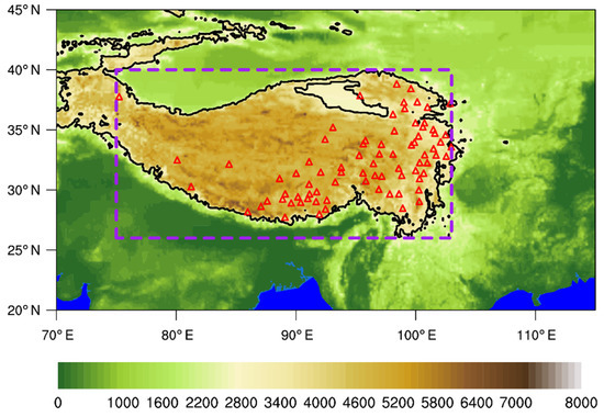
Figure 1.
Terrain height of the TP (shading; units: m). TP is defined as the region within 26–40°N and 75–103°E (purple dashed rectangle) where the terrain height exceeds 3000 m (black line). The red triangles show the location of automatic weather stations on the TP.
We used hourly 0.1° × 0.1° infrared brightness temperature observations from the Fengyun-2E geostationary meteorology satellites for 2013–2014 and from Fengyun-2G for 2015–2019. We also used the China Merged Precipitation Analysis (CMPA) dataset, which combines hourly rain gauge observations with the NOAA/Climate Prediction Center Morphing (CMORPH) precipitation product on a 0.1° × 0.1° grid. In general, more than 50% of the grid boxes with a 0.1° resolution in eastern China contain at least one rain gauge, whereas there is usually no station within a 500 km radius of the grid boxes in western China (west of 90°E). In these regions with sparsely distributed automatic weather stations, some unrealistic rainfall centers are usually depicted. Even so, this dataset in general has a smaller bias and root mean square error than other precipitation datasets, and it captures the major temporally varying features of hourly precipitation during the period of intense rainfall regardless of gauge density [43]. To analyze the atmospheric circulations, the hourly 0.25° × 0.25° European Center for Medium-Range Weather Forecasts Reanalysis 5 (ERA-5) dataset was used.
2.2. MCS Identification and Tracking Methods
Following the methods of Ai et al. [44], the infrared brightness temperature and precipitation data were used to identify and track MCSs via the following steps:
- (1)
- Step 1: cloud identification
Based on the infrared brightness temperature, we classify clouds into two categories: convective shield (CS, brightness temperature <240 K) and convective core (CC, brightness temperature <225 K).
- (2)
- Step 2: matching CS with precipitation
The rain associated with CS is defined as follows (Figure 2): An external rectangle (black dashed line) is drawn around each CS (orange contours), and a circle is drawn centered over the CS with a radius equal to the maximum distance from the centroid (red cross) to the four apexes of the bounding box. The precipitation in the black circle is defined as the rain matched to a CS.
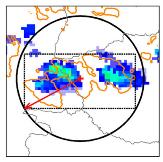
Figure 2.
Matching of precipitation to CS. The orange contour represents the region with an infrared brightness temperature of 240 K, and the red cross marks the centroid of the CS. The red arrow (radius) is the maximum distance from the centroid to the four apexes of the bounding box (black dashed rectangle). A circular search range (bold black circle) can then be drawn to find the associated rain (shading) within a CS (adapted from [44]).
- (3)
- Step 3: identification and tracking methods
An MCS is identified by a combination of satellite and precipitation information. The formation time (FT) of an MCS is defined as when the following four criteria are first met in three successive hours: ① the CC exists, ② the maximum rain intensity exceeds 2 mm·h−1 (this criterion is from the rain intensity range of weak deep convective precipitation over the TP [45]), ③ the area of CS is over 5000 km2 [10,46] and ④ the total area of the precipitation region is above 200 km2.
Starting from FT, the MCSs are tracked backward and forward based on the areal overlap method. A cloud at a later hour corresponds to the cloud at an earlier time if their CS overlapping area is more than 10%. The initiation time (IT) of the MCS is defined as the earliest time that satisfies the backward tracking criterion, and the dissipation time (DT) is defined as when the maximum rain intensity is lower than 2 mm·h−1 (Figure 3). If several clouds in the later hour meet this condition, the one with the largest overlapping area is considered to be the continuous MCS. If two or more MCSs merge together, then the merged MCS is assumed to be a continuation of the largest MCS and the smaller MCSs are terminated. When an MCS splits into several smaller parts, the largest part is assumed to be the continuous MCS and the smaller parts are assumed to be new MCSs if they satisfy the criteria of an MCS.
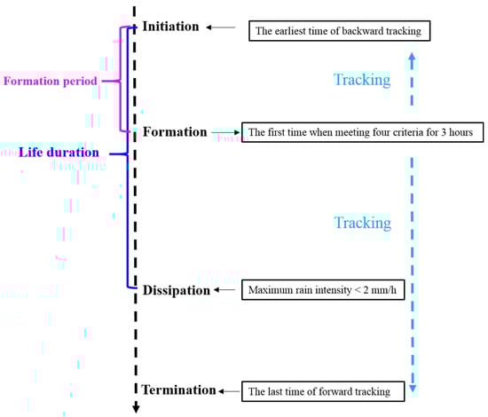
Figure 3.
Flow diagram showing the procedure for the identification and tracking of MCSs.
Previous studies have identified MCSs based on different infrared brightness temperatures. Machado et al. [15] used 245 and 218 K thresholds to define convective systems and the active deep convective cells embedded within the convective systems. Zheng et al. [17] used 221 K as the criterion to identify MCSs in China and its vicinity, and Mathon and Laurent [10] employed 233 and 213 K to analyze deep convection and the most active part of convective systems, respectively. There is no universal brightness temperature threshold for MCS identification, and changes within 5 K do not make a significant difference between the results [44]. The 240 and 225 K thresholds used for identifying MCSs in this study are derived from the distribution range of the infrared brightness temperature of deep weak convective precipitation over the TP [45], and introducing the precipitation criterion helps to reduce the misclassification of high cirrus clouds or stratus clouds with low rain rates as MCSs.
The tracking method used in this study is similar to that in [44], except that the infrared brightness temperature, rain intensity and area criteria are modified for the TP region. Compared with [47], both forward and backward tracking and the rain intensity are introduced in this study to improve the tracking processes. The areal overlap method is based on the assumption that temperature distribution and area of convective systems do not change strongly in a short time. The small overlapping rate used in this study enables the tracking of small convective clouds right after convective initiation. By testing, it was determined that the results were slightly affected when the overlapping rate was set to 20%.
- (4)
- Step 4: physical parameters
In order to characterize the MCSs’ features quantitatively, some life cycle physical parameters are introduced. The life duration that characterizes the time of activities of MCSs is calculated as the time between IT and DT. The formation period ratio (FPR) is the time between IT and FT divided by life duration and multiplied by 100%:
The formation speed of MCSs can be measured by FPR, and a smaller FPR represents a faster formation speed. The life duration and FPR for each MCS, as well as the minimum infrared brightness temperature (BTmin), the maximum rate intensity (Pmax), the maximum associated rain area (PAmax), the maximum CS area (CSAmax) and the maximum CC area (CCAmax) during MCS life cycle are examined.
2.3. Classification of MCSs
At any given hour, the location of the centroid of an MCS is taken as its position, and the direction of movement is determined by the line between its initiation and dissipation points. If the direction of movement lies between the northeast and southeast (45–135° clockwise from the true north), then it is defined as eastward moving. If the direction of movement lies between the southwest and southeast (135–225° clockwise from the true north), then it is defined as southward moving. If the direction of movement lies between southwest and northwest (225–315° clockwise from the true north), then it is defined as westward moving. Here, we define 103° E as the eastern boundary of the TP. If an MCS moves further east than 103° E, then it is considered to have vacated the TP. Based on their direction of movement and tracks, the MCSs initiated over the TP can be classified roughly into four types: (a) eastward moving out of the TP (EO), (b) southward moving (SM), (c) westward moving (WM) and (d) eastward moving but not out of the TP (EN), and SM, WM and EN are all defined as non-EOs.
3. Results
A total of 8820 MCSs were identified over the TP during seven summers, equivalent to about four MCSs per day, which demonstrates that MCSs are very active over the TP in summer. Of all the MCSs, there were 820 (9.3%) EOs, 1739 (19.7%) SMs, 1640 (18.6%) WMs and 4621 (52.4%) ENs. Therefore, the occurrence frequency of EOs is the lowest, while that of ENs is the highest.
3.1. Circulation and Environmental Features
In general, weather systems move along the direction of the mid-level mean flow, which is usually called “steering flow”. The mean zonal wind (U), meridional wind (V) and relative humidity (RH) of all MCS areas were therefore calculated from the ERA-5 reanalysis dataset to study the vertical distribution of circulation and environmental features of different types of MCSs. Figure 4a,b shows that the westerly (northerly) wind is strongest for EOs (SMs), which favors their eastward (southward) movement out of the TP. The differences in U and V among each type of MCS mainly appear in the upper troposphere, indicating that the movement of MCSs is mainly due to the mid- to high-level dynamic conditions. The U and V of ENs are both too small for them to move out from the TP, and the easterly wind in the low to middle troposphere contributes to the westward movement of WMs. The RH levels of EOs and SMs are greater than those of WMs and ENs (Figure 4c), because moisture is an essential factor in the development and maintenance of MCSs.
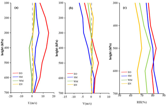
Figure 4.
Circulation and environmental features of each type of MCS. (a) Zonal winds; (b) meridional winds; (c) relative humidity. Gray, red, blue, green and yellow lines represent the zero value, EO, SM, WM and EN, respectively.
3.2. Spatial Distribution of Occurrence and Tracks
Figure 5 shows the spatial distribution of MCSs initiated over the TP. There was much more MCS activity over the southern TP than over the northern TP, with two centers of maximum activity along 30°N over the southern TP. The western center with two peaks was located over the southwestern TP around 85–90°E, and the eastern center was located over the southeastern TP near 100°E (Figure 5a), which is in agreement with previous work [30,35,36]. Most of the EOs were initiated over the southeastern TP east of 95°E (Figure 5b), especially at the eastern boundary of the TP, and the center of maximum activity was located near 30°N and 102°E. Most of the SMs were also initiated in this area, and the southwestern TP had a high frequency of SMs, although at a lower density (Figure 5c). Most WMs occurred in the western center near 90°E (Figure 5d), whereas the highest frequency of ENs occurred in the western center near 85°E, with a slightly weaker center over the southeastern TP (Figure 5e). Therefore, the southeastern center of activity over the TP was mainly due to EOs and SMs, whereas WMs and ENs mainly occurred over the western one.
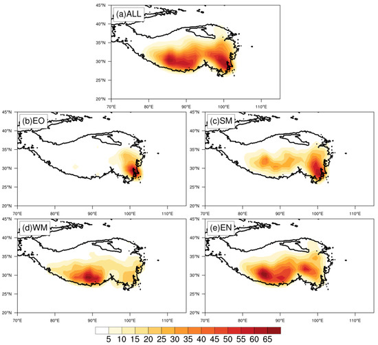
Figure 5.
Spatial distribution of MCS initiation over the TP on 1° × 1° grids. (a) All MCSs; (b) EOs; (c) SMs; (d) WMs; (e) ENs.
The spatial distribution of MCSs initiated in June, July and August is shown in the Supplementary Material. In June, there was much more MCS activity over the southeastern TP than over the southwestern TP. The western centers of SMs, WMs and ENs were greatly weakened. However, much more SMs, WMs and ENs occurred over the southwestern center in July and August than in June. From June to August, EOs always only occurred over the southeastern TP, and there was more SM (WM) activity over the southeastern (southwestern) TP than the other. The southeastern center with more ENs appeared in June, while the southwestern one was enhanced in July and August.
EOs mainly influenced the regions east of 90° E, and most of them affected southwestern China after they had vacated the TP (Figure 6a). Non-EOs affected almost all of the TP with shorter tracks, and they could vacate the TP in other directions. A total of 311 SMs moved southward out of the TP, and they moved mostly to the south of the TP after vacating the TP (Figure 6b). A total of 129 WMs moved westward out of the TP, and some even reached India (Figure 6c). The statistical results indicate that over 85% of MCSs dissipated within the TP.
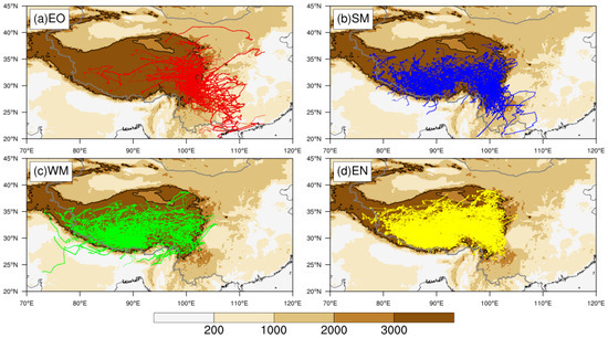
Figure 6.
Initiation location (points in color) and tracks (thin curves in color) of MCSs initiated over the TP. (a) EOs; (b) SMs; (c) WMs; (d) ENs. The shading area and the black line represent the terrain and the 3000 m terrain height, respectively.
3.3. Lifespan
The life duration distributions of SMs, WMs and ENs showed similar features but were different from the life duration distribution of EOs. During the whole summer, the mean life duration of EOs was ~22 h, nearly twice that of non-EOs (~12 h). About 78.9% of the non-EOs lasted less than 15 h, and the number of non-EOs with a life duration of more than 20 h was significantly reduced, whereas 70.1% of the EOs lasted longer than 15 h. In addition, 25% EOs lasted for more than 30 h, and very few non-EOs lasted this long (Figure 7a). In July, 40% EOs lasted longer than 30 h, and the corresponding proportions in June and August were 22% and 17% (Figure 7b–d), indicating that EOs with longer life duration are more likely to occur in July. By virtue of the westerly jet, no WMs lasted longer than 18 h in June. As most EOs were initiated near the east edge of the TP, it was much easier for them to move eastward out of the TP under stronger westerly wind conditions. Once they reached areas east of the TP with lower elevations, increased moisture supplement usually made them intensify and last longer.
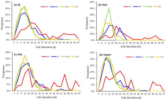
Figure 7.
Life duration distribution of EOs (red), SMs (blue), WMs (green) and ENs (yellow). (a) Whole summer; (b) June; (c) July; (d) August.
3.4. Temporal Variations
3.4.1. Annual Variations
Figure 8 shows the annual variation of MCS occurrence number from 2013 to 2019. The maximum occurrence number of MCSs was 1984 in 2016, and the minimum was 670 in 2019. In each year, nearly half of the MCSs were ENs, and the proportions of SMs and WMs both ranged between 10 and 20%. The proportion of EOs was the smallest and varied considerably, with a maximum of 12.48% in 2015 and a minimum of 8.31% in 2013.
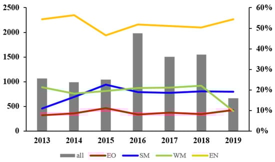
Figure 8.
Annual variation of MCS number (gray columns) and proportion of EOs (red), SMs (blue), WMs (green) and ENs (yellow) from 2013 to 2019.
3.4.2. Monthly Variations
The monthly variation of MCS number over the TP is shown in Figure 9. MCSs initiated in July and August accounted for over 80% of the total MCSs in summer, and most of the SMs and ENs (WMs) appeared in July (August), whereas the EOs showed an opposite trend. The proportion of EOs was much lower in July (7.2%) and August (6.43%) than in June (24.3%), which is consistent with previous results [35]. This remarkable monthly variation was mainly due to the variation in latitude of the westerly jet over the TP [26,48] and the enhancement of the South Asia high in July and August. The westerly jet at 200 hPa jumped from the southern to the northern TP with the onset of the monsoon in June, and the westerly wind over the TP was (not) favorable for EOs (WMs) moving eastward (westward) (Figure 10a). In July (August), the South Asia high was established over the TP and southeastern (southwestern) TP was under the northerly (easterly) winds, which favored the movement of SMs (WMs) (Figure 10b,c) [26]. Convective available potential energy (CAPE) is a crucial factor in the initiation and organization processes of MCSs. Figure 10e shows that, in July, there were two CAPE maximum centers over the southeastern and southwestern TP corresponding to the two initiation centers, and they were slightly larger than the CAPE maximum center in August (Figure 10f) and much larger than the CAPE maximum center in June (Figure 10d). A larger CAPE corresponded to more frequent MCS initiation, which indicated that CAPE is one of the most important factors that result in different numbers of MCSs in each month.
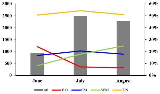
Figure 9.
Monthly variation of MCS number (gray columns) and proportion of EOs (red), SMs (blue), WMs (green) and ENs (yellow) from 2013 to 2019.
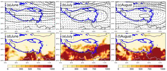
Figure 10.
Mean geopotential height (black lines, units: dagpm), wind fields at 200 hPa (top panel) and CAPE (bottom panel) in (a,d) June, (b,e) July and (c,f) August.
3.4.3. Diurnal Variations
The UTC was converted to local standard time (LST) to investigate the diurnal variation features of MCSs because the Tibetan Plateau spans multiple time zones. The combined non-EO was used because the SMs, WMs and ENs showed similar trends. The IT frequency increased rapidly from 12:00 LST and peaked at 13:00–16:00 LST due to the solar radiation, and then decreased significantly from 18:00 LST to the next day (Figure 11a), which is consistent with previous reports [17,35]. The maximum frequency of EOs occurred at around 15:00 LST, and the corresponding time for non-EOs happened an hour later. About 70.8% of EOs were initiated in the afternoon (12:00–18:00 LST), and the corresponding frequency of non-EOs was 58.1%, indicating that EOs need more solar radiation for initiation than non-EOs.
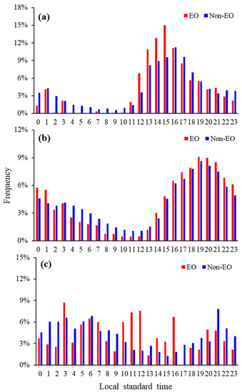
Figure 11.
Diurnal variation of EOs (red) and non-EOs (blue) from 2013 to 2019. (a) Initiation time; (b) formation time; (c) dissipation time.
The FT frequency of EOs and non-EOs (Figure 11b) showed the same trend as IT, but occurring a few hours later. The frequency of EOs (38%) was close to that of non-EOs (36%) at night (22:00–06:00 LST) and was much more than that of IT (12% and 23% for EOs and non-EOs, respectively), which indicates that the MCS formation processes depend on the environmental circulation and other factors besides solar radiation. The DT frequency peak for EOs (non-EOs) occurred around 10:00–12:00 (01:00–06:00) LST (Figure 11c), corresponding to the results calculated from IT and the mean life duration.
3.5. Physical Parameters
There was no obvious difference among the physical parameters of SMs, WMs and ENs, whereas EOs showed some unique characteristics. The distribution of BTmin showed that nearly 50% of EOs reached a BTmin less than the average value of 208 K (Figure 12a), whereas only 20% of non-EOs did so and the average was 214 K (Figure 12g,m,s), which means that non-EOs were less deep than EOs. The mean Pmax of EOs was 41 mm•h−1, and nearly half of them experienced a maximum rain rate over 40 mm•h−1 (Figure 12b). The Pmax of non-EOs was much less, with an average of 20–26 mm•h−1 (Figure 12h,n,t). Note that the Pmax features of MCSs over the TP had not been examined before, because the temporal–spatial resolution of daily rain data and accuracy of satellite precipitation products used in previous studies were too coarse to provide sufficient details. Over 70% of EOs and less than 50% of non-EOs spent two-fifths of their life duration undergoing the formation processes, with averages of 26% and around 40%, respectively, indicating that EOs developed faster (Figure 12c,i,o,u). PAmax and CSAmax mainly ranged between 104 and 106 km2, both with an expected value of over 105 km2 for EOs, which are significantly greater than those of non-EOs (Figure 12d,e,j,k,p,q,v,w). CCAmax mainly ranged between 103 and 105 km2, and 13% (2%) of EOs (non-EOs) exceeded 105 km2 (Figure 12f,l,r,x).
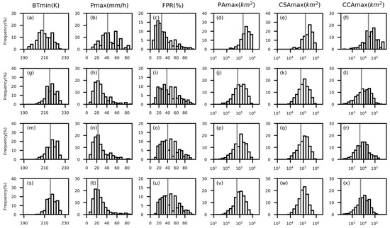
Figure 12.
Distribution of physical parameters of MCSs. (a–f) EOs; (g–l) SMs; (m–r) WMs; (s–x) ENs. The gray vertical lines represent the average value, and BTmin, Pmax, FPR, PAmax, CSAmax and CCAmax represent the lowest infrared brightness temperature, max precipitation intensity, formation percentage, max precipitation area, max CS area and max CC area, respectively.
The spatial distribution of BTmin and Pmax are shown in Figure 13 and Figure 14. For all MCSs, both BTmin and Pmax presented spatial patterns similar to those of MCS occurrences (Figure 13a and Figure 14a). The BTmin maximum center of each type of MCS was located slightly downstream of the moving direction to the initiation area (Figure 13b–e), and the Pmax maximum center further was located slightly downstream of the moving direction to the BTmin maximum center (Figure 14b–e). Due to the more abundant moisture over the lower reaches of the TP, rain intensity often reached its peak when EOs moved eastward out of the TP.
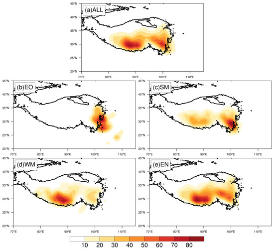
Figure 13.
Spatial distribution of BTmin over the TP on 1° × 1° grids. (a) All MCSs; (b) EOs; (c) SMs; (d) WMs; (e) ENs.
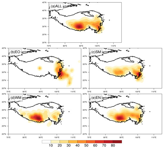
Figure 14.
Spatial distribution of Pmax over the TP on 1° × 1° grids. (a) All MCSs; (b) EOs; (c) SMs; (d) WMs; (e) ENs.
Compared with non-EOs, EOs had a lower cloud-top temperature, greater rainfall intensity, longer life duration, more rapid development, larger areas of rainfall and convective clouds, longer tracks and a wider influence range, indicating that EOs were more vigorous. The BTmin and Pmax maximum centers of each type of MCS were located slightly downstream of the moving direction to the initiation area, and the maximum rain intensity of EOs was located east of the eastern boundary of the TP.
The differences in occurrence time (Δt) between BTmin and Pmax are shown in Figure 15. SMs, WMs and ENs showed similar features in each month. Among most events, the Δt values ranged between –12 and 6 h, and BTmin occurred earlier than Pmax for more than 80% of MCSs. A Δt of between −6 and 3 h was observed for 90% of non-EOs but only 80% of EOs. The proportion of EOs with positive Δt is obviously larger than that of non-EOs. Results indicate that the peak in precipitation was usually followed by a minimum in brightness temperature over the TP. The occurrence of BTmin ahead of Pmax is in agreement with what was obtained from a single cell [49], which can be explained by intense precipitation usually resulting from a rapid vertical updraft. The remaining MCSs for which BTmin was followed by Pmax may be multi-cell convective systems. When some MCSs merge together, the updraft of the whole system may continue to grow after the precipitation reaches its maximum [44]. This may be a possible explanation for long-lasting EOs.
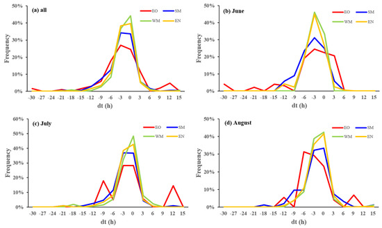
Figure 15.
Difference in occurrence time (Δt) between BTmin and Pmax for EOs (red), SMs (blue), WMs (green) and ENs (yellow). Negative Δt means BTmin occurs earlier than Pmax. (a) Whole summer; (b) June; (c) July; (d) August.
4. Discussions
In this study, we found that no more than 15% of MCSs moved out of the TP, and EOs accounted for 9.3%, which is similar to the 6.6% reported previously [35]. These results are much less than the value of 47% found in [36] and the value of 49% found in [26]. The mean life duration in this study was 12 h, which is much shorter than the 36 h found in [36] but a few hours longer than that found in [26]. EOs in this study mainly influenced the regions east of 90° E, whereas Hu et al. [26] indicated that some EOs may propagate to the east of Japan. These differences may be a result of the use of hourly satellite data and the precipitation criteria in the definition of MCSs in this study rather than the three-hourly data used elsewhere. The usage of coarse-resolution data may misclassify two independent MCSs into one and thus “prolong” the life duration and tracks. Moreover, as the zenith angle of the Fengyun satellite is less than that of other satellites, the hourly data used in this study should be more reliable for studying MCSs over the TP.
We used a strict definition of MCSs in this study based on both the rain intensity and the requirement of meeting four criteria in three successive hours. More physical parameters than in previous studies [35] were introduced to investigate the detailed statistical features of different types of MCSs. As there are fewer automatic weather stations over the western TP, the CMPA is mainly composed of the CMORPH precipitation product, and it may be inaccurate to some extent.
When EOs move out of the TP, they may induce a southwest vortex around the Sichuan Basin and further intensify rainfall downstream. In most cases, with the eastward movement, the southwest vortex impacts not only its genesis area but also the middle and lower reaches of the Yangtze River. The contributions of the dynamic and thermal processes to the formation of a southwest vortex may be complicated and vary in different cases. The relationship and interaction between EOs and southwest vortex will be investigated in future research.
5. Conclusions
Based on the hourly Fengyun satellite infrared brightness temperature data and CMPA precipitation data, MCSs initiated over the TP in summer from 2013 to 2019 were examined statistically in this study. By investigating the occurrence frequency, life duration, temporal and spatial distribution, physical parameters and circulation and environmental features, some new findings were obtained.
During the seven summers, 8820 MCSs formed over the TP. Based on the direction of movement and tracks, MCSs were classified as EOs, SMs, WMs and ENs. The SMs, WMs and ENs showed similar features. Of all the MCSs, EOs, SMs, WMs and ENs accounted for 9.3%, 19.7%, 18.6% and 52.4%, respectively, and the mean life duration of EOs was about 22 h, nearly twice that of the non-EOs (SMs, WMs, ENs; about 12 h). The number of MCSs initiated over the TP varied annually, with the maximum number of 1984 in 2016 and the minimum number of 670 in 2019, while the corresponding years for EOs were 2015 (maximum) and 2013 (minimum). Most MCSs occurred in July and August except for EOs (June), and the maximum frequency for EOs occurred at around 15:00 LST, which is an hour earlier than non-EOs.
There was much more MCS activity over the southern TP than the northern TP, with two maximum frequency centers along 30° N over the southwestern and southeastern TP. MCSs that formed west of 95° E could rarely move eastward out of the TP. EOs and SMs were mainly initiated over the southeastern center, whereas WMs and ENs mainly took place over the western one. EOs mainly influenced the regions east of 90° E, and most of them affected southwestern China after vacating the TP. Moreover, SMs and WMs were also able to move out of the TP. Almost 15% of all MCSs were able to leave this region.
Based on the lifetime physical parameters, some key features of different types of MCSs can be illustrated. EOs usually have a lower cloud-top temperature, greater rainfall intensity, longer life duration, more rapid development, larger areas of rainfall and convective clouds, longer tracks and wider influence range, indicating that EOs are more vigorous. The BTmin and Pmax maximum centers of each type of MCS were located slightly downstream of the moving direction to the initiation area, and the maximum rain intensity of EOs was located east of the eastern boundary of the TP. The environmental circulations associated with different types of MCSs differ remarkably from each other. The movement of MCSs is mainly due to the mid- to high-level dynamic conditions, and moisture is an essential factor in the development and maintenance of MCSs.
Supplementary Materials
The following are available online at https://www.mdpi.com/article/10.3390/rs13091652/s1, Figure S1: Spatial distribution of MCSs initiation over the TP on 1°×1° grids in June. (a) All MCSs; (b) EOs; (c) SMs; (d) WMs; (e) ENs. Figure S2: Spatial distribution of MCSs initiation over the TP on 1°×1° grids in June. (a) All MCSs; (b) EOs; (c) SMs; (d) WMs; (e) ENs. Figure S3: Spatial distribution of MCSs initiation over the TP on 1°×1° grids in August. (a) All MCSs; (b) EOs; (c) SMs; (d) WMs; (e) ENs.
Author Contributions
Conceptualization, X.Z. (Xiaoyong Zhuge), S.Y. and Y.C.; methodology, X.Z. (Xidi Zhang) and W.S.; software, X.Z. (Xidi Zhang) and W.S.; validation, X.Z. (Xiaoyong Zhuge), Y.C., T.C. and S.Z.; formal analysis, X.Z. (Xidi Zhang) and X.Z. (Xiaoyong Zhuge); investigation, X.Z. (Xidi Zhang), S.Y. and Y.C.; resources, X.Z. (Xidi Zhang); data curation, X.Z. (Xidi Zhang); writing—original draft preparation, X.Z. (Xidi Zhang); writing—review and editing, X.Z. (Xidi Zhang), X.Z. (Xiaoyong Zhuge) and Y.C.; visualization, X.Z. (Xidi Zhang) and W.S.; supervision, X.Z. (Xiaoyong Zhuge), Y.C. and Y.W.; project administration, X.Z. (Xiaoyong Zhuge), S.Y., Y.C. and Y.W.; funding acquisition, X.Z. (Xiaoyong Zhuge), S.Y., Y.C. and T.C. All authors have read and agreed to the published version of the manuscript.
Funding
This research was funded by the National Key Research and Development Program of China (2018YFC1505704 and 2018YFC1505705), the National Natural Science Foundation of China (91837207, 91937301, 41930972), the Innovative Development Special Project of China Meteorological Administration (CXFZ2021Z033) and the Special Project of heavy rain forecasting expert innovation team of China Meteorological Administration (CMACXTD002-3).
Institutional Review Board Statement
Not applicable.
Informed Consent Statement
Not applicable.
Data Availability Statement
Not applicable.
Acknowledgments
We appreciate the Fengyun satellite data provided by the National Satellite Meteorological Center of China Meteorological Administration (http://satellite.nsmc.org.cn/PortalSite/Data/Satellite.aspx, accessed on 13 July 2019). We also would like to thank the National Meteorological Information Center of China Meteorological Administration for the CMPA precipitation products (http://data.cma.cn/data/cdcdetail/dataCode/SEVP_CLI_CHN_MERGE_CMP_PRE_HOUR_GRID_0.10.html, accessed on 13 July 2019) and the European Center for Medium-Range Weather Forecasts for the ERA-5 reanalysis data (https://cds.climate.copernicus.eu/cdsapp#!/home, accessed on 13 July 2019). Last but not least, we thank the invaluable comments and suggestions by the anonymous reviewers that helped to greatly improve the quality of our manuscript.
Conflicts of Interest
The authors declare no conflict of interest.
References
- Nesbitt, S.W.; Cifelli, R.; Rutledge, S.A. Storm Morphology and Rainfall Characteristics of TRMM Precipitation Features. Mon. Wea. Rev. 2006, 134, 2702–2721. [Google Scholar] [CrossRef]
- Rasmussen, K.L.; Chaplin, M.M.; Zuluaga, M.D.; Houze, R.A., Jr. Contribution of Extreme Convective Storms to Rainfall in South America. J. Hydrometeorol. 2016, 17, 353–367. [Google Scholar] [CrossRef]
- Carvalho, L.M.V.; Jones, C. A Satellite Method to Identify Structural Properties of Mesoscale Convective Systems Based on Maximum Spatial Correlation Tracking Technique (MASCOTTE). J. Appl. Meteorol. 2001, 40, 1683–1701. [Google Scholar] [CrossRef]
- Vila, D.A.; Machado, L.A.T.; Laurent, H.; Velasco, I. Forecast and Tracking the Evolution of Cloud Clusters (ForTraCC) Using Satellite Infrared Imagery: Methodology and Validation. Wea. Forecast. 2008, 23, 233–245. [Google Scholar] [CrossRef]
- Goyens, C.; Lauwaet, D.; Schröder, M.; Demuzere, M.; Van Lipzig, N.P.M. Tracking mesoscale convective systems in the Sahel: Relation between cloud parameters and precipitation. Int. J. Climatol. 2011, 32, 1921–1934. [Google Scholar] [CrossRef]
- Aspliden, C.I.; Tourre, Y.; Sabine, J.B. Some Climatological Aspects of West African Disturbance Lines During GATE. Mon. Wea. Rev. 1976, 104, 1029–1035. [Google Scholar] [CrossRef][Green Version]
- Desbois, M.; Kayiranga, T.; Gnamien, B.; Guessous, S.; Picon, L. Characterization of Some Elements of the Sahelian Climate and Their Interannual Variations for July 1983, 1984 and 1985 from the Analysis of METEOSAT ISCCP data. J. Climate 1988, 1, 867–904. [Google Scholar] [CrossRef]
- Payne, S.W.; McGarry, M.M. The Relationship of Satellite Inferred Convective Activity to Easterly Waves Over West Africa and the Adjacent Ocean During Phase III of GATE. Mon. Wea. Rev. 1977, 105, 413–420. [Google Scholar] [CrossRef]
- Houze, R.A., Jr. Observed structure of mesoscale convective systems and implications for large scale heating. Quart. J. Roy. Meteorol. Soc. 1989, 115, 425–461. [Google Scholar] [CrossRef]
- Mathon, V.; Laurent, H. Life cycle of Sahelian mesoscale convective cloud systems. Quart. J. Roy. Meteorol. Soc. 2001, 127, 377–406. [Google Scholar] [CrossRef]
- Mathon, V.; Diedhiou, A.; Laurent, H. Relationship between easterly waves and mesoscale convective systems over the Sahel. Geophys. Res. Lett. 2002, 29, 1216. [Google Scholar] [CrossRef]
- Mapes, B.E. Gregarious tropical convection. J. Atmos. Sci. 1993, 50, 2026–2037. [Google Scholar] [CrossRef]
- Mapes, B.E.; Houze, R.A., Jr. Cloud clusters and superclusters over the oceanic warm pool. Mon. Wea. Rev. 1993, 121, 1398–1415. [Google Scholar] [CrossRef]
- Chen, S.S.; Houze, R.A., Jr.; Mapes, B.E. Multiscale Variability of Deep Convection in Relation to Large-Scale Circulation in TOGA COARE. J. Atmos. Sci. 1996, 53, 1380–1409. [Google Scholar] [CrossRef]
- Machado, L.A.T.; Rossow, W.B.; Guedes, R.L.; Walker, A.W. Life cycle variations of mesoscale convective systems over the Americas. Mon. Wea. Rev. 1998, 126, 1630–1654. [Google Scholar] [CrossRef]
- Pope, M.; Jakob, C.; Reeder, M.J. Convective systems of the north Australian monsoon. J. Climate 2008, 21, 5091–5112. [Google Scholar] [CrossRef][Green Version]
- Zheng, Y.G.; Chen, J.; Zhu, P.J. Climatological distribution and diurnal variation of mesoscale convective systems over China and its vicinity during summer. Chin. Sci. Bull. 2008, 53, 1574–1586. [Google Scholar] [CrossRef]
- Zheng, L.L.; Sun, J.H.; Zhang, X.L.; Liu, C.H. Organizational Modes of Mesoscale Convective Systems over Central East China. Wea. Forecast. 2013, 28, 1081–1098. [Google Scholar] [CrossRef]
- Meng, Z.Y.; Yan, D.C.; Zhang, Y.J. General Features of Squall Lines in East China. Mon. Wea. Rev. 2013, 141, 1629–1647. [Google Scholar] [CrossRef]
- Shen, R.; Reiter, E.R.; Bresch, J.F. Numerical Simulation of the Development of Vortices over the Qinghai-Xizang (Tibet) Plateau. Meteorol. Atmos. Phys. 1986, 35, 70–95. [Google Scholar] [CrossRef]
- Wang, W.; Kuo, Y.H.; Warner, T.T. A Diabatically Driven Mesoscale Vortex in the Lee of the Tibetan Plateau. Mon. Wea. Rev. 1993, 121, 2542–2561. [Google Scholar] [CrossRef]
- Zhao, P.; Xu, X.D.; Chen, F.; Guo, X.L.; Zheng, X.D.; Liu, L.P.; Hong, Y.; Li, Y.Q.; La, Z.; Peng, H.; et al. The Third Atmospheric Scientific Experiment for Understanding the Earth-Atmosphere Coupled System over the Tibetan Plateau and Its Effects. Bull. Amer. Meteor. Soc. 2018, 99, 757–776. [Google Scholar] [CrossRef]
- Tao, S.Y.; Ding, Y.H. Observational evidence of the influence of the Qinghai-Xizang (Tibet) Plateau on the occurrence of heavy rain and severe convective storms in China. Bull. Amer. Meteor. Soc. 1981, 62, 23–30. [Google Scholar] [CrossRef]
- Hu, L.; Li, Y.D.; Fu, R.; He, J.H. The relationship between mobile mesoscale convective systems over Tibetan Plateau and the rainfall over eastern China in summer. Plateau Meteor. 2008, 27, 301–309. (In Chinese) [Google Scholar]
- Fu, S.M.; Sun, J.H.; Zhao, S.X.; Li, W.L. The impact of eastward propagation of convective systems over the Tibetan Plateau on southwest vortex formation in summer. Atmos. Oceanic Sci. Lett. 2010, 3, 51–57. [Google Scholar]
- Hu, L.; Deng, D.F.; Gao, S.T.; Xu, X.D. The seasonal variation of Tibetan convective systems: Satellite observation. J. Geophys. Res. Atmos. 2016, 121, 5512–5525. [Google Scholar] [CrossRef]
- Wang, J.Y.; Wang, X.F.; Wang, X.K.; Cui, C.G. Statistical characteristics of eastward propagation of cloud clusters from the Tibetan Plateau and mesoscale convective systems embedded in these cloud clusters. Chin. J. Atmos. Sci. 2019, 43, 1019–1040. (In Chinese) [Google Scholar]
- Zhang, S.L.; Tao, S.Y.; Zhang, Q.Y.; Zhang, X.L. Meteorological and hydrological characteristics of severe flooding in China during the summer of 1998. J. Appl. Meteor. Sci. 2001, 12, 442–457. (In Chinese) [Google Scholar]
- Zhuo, G.; Xu, X.D.; Chen, L.S. Instability of eastward movement and development of convective cloud clusters over Tibetan Plateau. J. Appl. Meteor. Sci. 2002, 13, 447–456. (In Chinese) [Google Scholar]
- Jiang, J.X.; Fan, M.Z. Convective clouds and mesoscale convective systems over the Tibetan Plateau in summer. Chin. J. Atmos. Sci. 2002, 26, 263–270. (In Chinese) [Google Scholar]
- Zhang, S.L.; Tao, S.Y. The influence of Tibetan Plateau on weather anomalies over Changjiang River in 1998. Acta. Meteorol. Sin. 2002, 60, 442–452. (In Chinese) [Google Scholar]
- Xu, X.D.; Chen, L.S. Advances of the study on Tibetan Plateau experiment of atmospheric sciences. J. Appl. Meteor. Sci. 2006, 17, 756–772. (In Chinese) [Google Scholar]
- Shan, Y.; Lin, H.; Fu, W.C.; Jiang, J.X.; Huang, Q. The features of MCS during its initiation over Tibetan Plateau in summer. J. Trop. Meteorol. 2003, 19, 61–66. (In Chinese) [Google Scholar]
- Jiang, J.X.; Xiang, X.K.; Fan, M.Z. The spatial and temporal distributions of severe mesoscale convective systems over Tibetan Plateau in summer. J. Appl. Meteor. Sci. 1996, 7, 473–478. (In Chinese) [Google Scholar]
- Mai, Z.; Fu, S.M.; Sun, J.H.; Hu, L.; Wang, X.M. Key statistical characteristics of the mesoscale convective systems generated over the Tibetan Plateau and their relationship to precipitation and southwest vortices. Int. J. Climatol. 2021, 41, E875–E896. [Google Scholar] [CrossRef]
- Li, Y.D.; Wang, Y.; Song, Y.; Hu, L.; Gao, S.T.; Fu, R. Characteristics of summer convective systems initiated over the Tibetan Plateau. Part I: Origin, track, development, and precipitation. J. Appl. Meteorol. Climatol. 2008, 47, 2769–2965. [Google Scholar]
- Hu, L.; Deng, D.F.; Xu, X.D.; Zhao, P. The regional differences of Tibetan convective systems in boreal summer. J. Geophys. Res. Atmos. 2017, 122, 7289–7299. [Google Scholar] [CrossRef]
- Liu, Y.; Yao, X.P.; Fei, J.F.; Yang, X.R.; Sun, J. Characteristics of mesoscale convective systems during the warm season over the Tibetan Plateau based on FY-2 satellite datasets. Int. J. Climatol. 2021, 41, 2301–2315. [Google Scholar] [CrossRef]
- Xu, W.X.; Zipser, E.J. Diurnal variations of precipitation, deep convection, and lightning over and east of the Eastern Tibetan Plateau. J. Climate 2011, 24, 448–465. [Google Scholar] [CrossRef]
- Feng, Z.; Dong, X.Q.; Xi, B.K.; McFarlane, S.A.; Kennedy, A.; Lin, B.; Minnis, P. Life cycle of midlatitude deep convective systems in a Lagrangian framework. J. Geophys. Res. Atmos. 2012, 117, D23201. [Google Scholar] [CrossRef]
- Xu, W.X. Precipitation and convective characteristics of summer deep convection over East Asia observed by TRMM. Mon. Wea. Rev. 2013, 141, 1577–1592. [Google Scholar] [CrossRef]
- Yuan, J.; Houze, R.A., Jr. Global variability of mesoscale convective system anvil structure from A-Train satellite data. J. Climate 2010, 23, 5864–5888. [Google Scholar] [CrossRef]
- Shen, Y.; Zhao, P.; Pan, Y.; Yu, J.J. A high spatiotemporal gauge-satellite merged precipitation analysis over China. J. Geophys. Res. Atmos. 2014, 119, 3063–3075. [Google Scholar] [CrossRef]
- Ai, Y.F.; Li, W.B.; Meng, Z.Y.; Li, J. Life Cycle Characteristics of MCSs in Middle East China Tracked by Geostationary Satellite and Precipitation Estimates. Mon. Weather Rev. 2016, 144, 2517–2530. [Google Scholar] [CrossRef]
- Pan, X.; Fu, Y.F. Analysis on Climatological Characteristics of Deep and Shallow Precipitation Cloud in Summer over Qinghai-Xizang Plateau. Plateau Meteor. 2015, 34, 1191–1203. (In Chinese) [Google Scholar]
- Yang, R.Y.; Zhang, Y.C.; Sun, J.H.; Fu, S.M.; Li, J. The characteristics and classification of eastward-propagating mesoscale convective systems generated over the second-step terrain in the Yangtze River Valley. Atmos. Sci. Lett. 2019, 20, e874. [Google Scholar] [CrossRef]
- Schröder, M.; König, M.; Schmetz, J. Deep convection observed by the Spinning Enhanced Visible and Infrared Imager on board Meteosat 8: Spatial distribution and temporal evolution over Africa in summer and winter 2006. J. Geophys. Res. Atmos. 2009, 114, D05109. [Google Scholar] [CrossRef]
- Li, C.Y.; Wang, Z.T.; Lin, S.Z.; Cho, H.R. The relationship between East Asia summer monsoon activity and northward jump of the upper westerly jet location. Chin. J. Atmos. Sci. 2004, 28, 641–658. (In Chinese) [Google Scholar]
- Houze, R.A., Jr. Mesoscale convective systems. Rev. Geophys. 2004, 42, RG4003. [Google Scholar] [CrossRef]


Publisher’s Note: MDPI stays neutral with regard to jurisdictional claims in published maps and institutional affiliations. |
© 2021 by the authors. Licensee MDPI, Basel, Switzerland. This article is an open access article distributed under the terms and conditions of the Creative Commons Attribution (CC BY) license (https://creativecommons.org/licenses/by/4.0/).