Article

Assessing Marginal Shallow-Water Bathymetric Information Content of Lidar Sounding Attribute Data and Derived Seafloor Geomorphometry

Centre for Coastal and Ocean Mapping and Joint Hydrographic Centre, University of New Hampshire, Durham, NH 03824, USA
*
Author to whom correspondence should be addressed.
Remote Sens. 2021, 13(9), 1604; https://doi.org/10.3390/rs13091604
Submission received: 16 February 2021 / Revised: 2 April 2021 / Accepted: 15 April 2021 / Published: 21 April 2021
(This article belongs to the Special Issue Monitoring Aquatic Environments Using LiDAR)

Abstract

:
Shallow-water depth estimates from airborne lidar data might be improved by using sounding attribute data (SAD) and ocean geomorphometry derived from lidar soundings. Moreover, an accurate derivation of geomorphometry would be beneficial to other applications. The SAD examined here included routinely collected variables such as sounding intensity and fore/aft scan direction. Ocean-floor geomorphometry was described by slope, orientation, and pulse orthogonality that were derived from the depth estimates of bathymetry soundings using spatial extrapolation and interpolation. Four data case studies (CSs) located near Key West, Florida (United States) were the testbed for this study. To identify bathymetry soundings in lidar point clouds, extreme gradient boosting (XGB) models were fitted for all seven possible combinations of three variable suites—SAD, derived geomorphometry, and sounding depth. R2 values for the best models were between 0.6 and 0.99, and global accuracy values were between 85% and 95%. Lidar depth alone had the strongest relationship to bathymetry for all but the shallowest CS, but the SAD provided demonstrable model improvements for all CSs. The derived geomorphometry variables contained little bathymetric information. Whereas the SAD showed promise for improving the extraction of bathymetry from lidar point clouds, the derived geomorphometry variables do not appear to describe geomorphometry well.

1. Introduction

As airborne lidar (‘light detection and ranging’) data become increasingly used for shallow-water bathymetric mapping (less than about 17 m depth), the need for efficient and accurate methods to separate bathymetric signals from noise in lidar data remains a challenge. A number of conceptual approaches for waveform lidar data were described in [1]: (1) mathematical approximation, (2) heuristic methods, (3) statistical approaches, and (4) deconvolution methods. Furthermore, some research has suggested that MBES (employed abbreviations are defined initially in the text and are also presented in at the end of this article) sonar and bathymetric lidar data can produce comparable average point accuracies under certain conditions (e.g., [2]). The high data volumes of waveform lidar data, however, result in slower processing than is possible with lidar point data. However, well-researched methods of extracting ocean bathymetry operationally from lidar point data have not been established.
The overarching context of the present research is therefore the operational extraction of bathymetry from lidar point clouds for shallow water. This paper specifically focuses on extracting bathymetry from currently unexploited information recorded for, or derivable from, ‘discrete’ or ‘point’ lidar data, i.e., not waveform data. The analytical framework is the improvement of a heuristic algorithm developed for MBES sonar data adapted to lidar pulse returns—or ‘soundings’ in ocean mapping parlance.
The subject algorithm is density-based and known as CHRT (CUBE with hierarchical resolution techniques [3,4]; another density-based algorithm that employs a random consensus filter [5] was described in [6,7]). CHRT establishes a grid of ‘estimation nodes’ (ENs) over an area of interest and, conceptually, uses the distance-defined ‘neighboring’ soundings around each EN to produce a depth frequency histogram that is conceptually equivalent to a waveform for a single lidar pulse. Individual histograms are usually multi-modal with each mode defining a depth ‘hypothesis.’ Figure 1 shows a fictitious example for a single EN for three different depths. In the shallow and mid-depth areas (Figure 1a,b), the hypotheses indicating the ocean floor contain the largest number of soundings, but for the shallow EN, there is considerable overlap between the bathymetry hypothesis and the non-bathymetry hypotheses. The depth of the deep area (Figure 1c) approaches the limit of lidar penetration; this results in the non-bathymetry hypotheses having the greatest number of soundings and being widely separate from the bathymetry hypotheses. Embedded in CHRT are disambiguation rules that determine which of an EN’s hypotheses is the most likely depth.
Density-based algorithms such as CHRT employ only the depth and uncertainty estimate reported for each lidar sounding/pulse return. This is clearly sensible since depth is likely to strongly indicate if a sounding is bathymetry or not, i.e., Bathy or NotBathy. Additionally associated with each sounding, however, are metadata such as the intensity of a sounding. These ‘sounding attribute data’ (SAD) are either collected during acquisition or can be derived post-acquisition. If such SAD relate to the bathymetric information content of soundings, they might be used to improve the disambiguation rules in CHRT, thereby producing more accurate bathymetric charts.
Another type of SAD that, in principle, can be derived is the geomorphometric characteristics of the ocean floor. It has been established that ocean bottom characteristics have important impacts on lidar reflectance [8] and passive optical data [9] for depth detection, as well as a number of other applications (e.g., [10,11]). Hence, there is considerable interest in geomorphometry beyond bathymetric mapping [12], e.g., ocean currents [13], ocean mixing [14], and biotic species distributions [15]. Using lidar data, the authors of [16,17] were able to characterize the rugosity of ocean bottoms in shallow waters using full waveform lidar. And using simulated lidar waveform data, the authors of [18] demonstrated that bottom reflectance and incident scan angle impact the accuracy of depth estimates from full waveform lidar, with bottom characteristics being the more important of the two factors. Exploring whether comparable results could be achieved using the discrete lidar data is the subject of the present research.
A major challenge in using point lidar data to extract ocean geomorphometry is the sparsity of Bathy soundings as one approaches the depth limit of lidar penetration (i.e., about 17 m). This was noted in the introduction to a special issue of Geosciences on geomorphometry [19], which also presented a summary of methods examined to address this with a focus on sonar data. As the number of Bathy soundings decrease and the distance between them increases, the ability to reliably characterize geomorphometry decreases. However, given that airborne lidar is the only current sensing technology that provides high resolution data for shallow water, the need for methods that provide geographically complete geomorphometric coverage from lidar point clouds has been recognized since at least 2012 [20].
The challenge of meaningfully describing geomorphometry in areas nearing the limits of lidar penetration is considerable. Lidar pulse returns with a high certainty of truly representing bathymetry can be sparse or non-existent resulting in large gaps in spatial coverage. Hence to overcome these limits, one must employ both spatial interpolation to fill in gaps between known points of bathymetry and extrapolation to artificially extend the limits of data. Both methods rely on explicit and implicit assumptions about bathymetry between known points and beyond.
The study reported here has a strategic goal of facilitating the production of maps of shallow water ocean floor geomorphometry from lidar point data to produce more accurate bathymetric maps. The developed approach applies extrapolation and spatial interpolation to lidar soundings classified as Bathy (by the data provider NOAA—the United States National Oceanic and Atmospheric Administration).
The signal strength present in various types and combinations of SAD metadata was evaluated by first fitting a classificatory model to the Bathy or NotBathy NOAA classification of each lidar sounding by using depth alone as a predictor. This provided a ‘null model’ against which the standalone and marginal contributions of pulse-return SAD and geomorphometric SAD could be compared using model goodness-of-fit and a variety of classification accuracy statistics. If either type of SAD alone produced a better model than the null model or if either/both improved the null model, classification models could be incorporated into operational workflows that enhance the existing disambiguation rules employed in density-based algorithms such as CHRT. Furthermore, a demonstration that derived geomorphometric SAD contribute to improved depth estimates implies that the developed methods produce ocean bottom descriptors that are able to describe actual geomorphometry. Thus, this article evaluated the absolute and marginal strengths of the bathymetric signal in different types and combinations of SAD metadata, including geomorphometry derived using spatial interpolation and extrapolation.

2. Materials and Methods

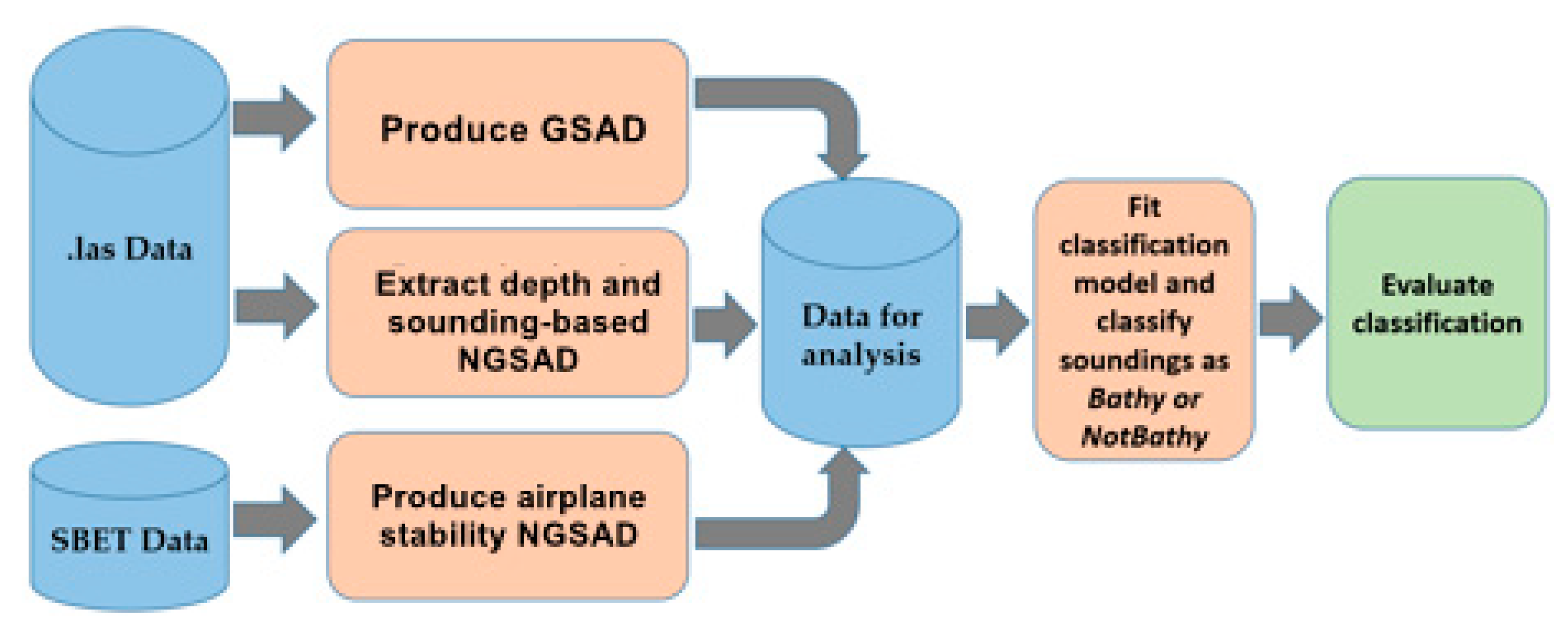
Figure 2 provides a schematic of the data and process flow of this study; details are discussed in subsequent sections. This research design required data extraction for both types of SAD, the fitting of an ML model, and the evaluation of the utility of the different types of SAD to determine the relative contributions of the non-geomorphometric SAD (NGSAD), the geomorphometric SAD (GSAD), and the ocean depth for each lidar point return.

2.1. Study Area and Instrumentation

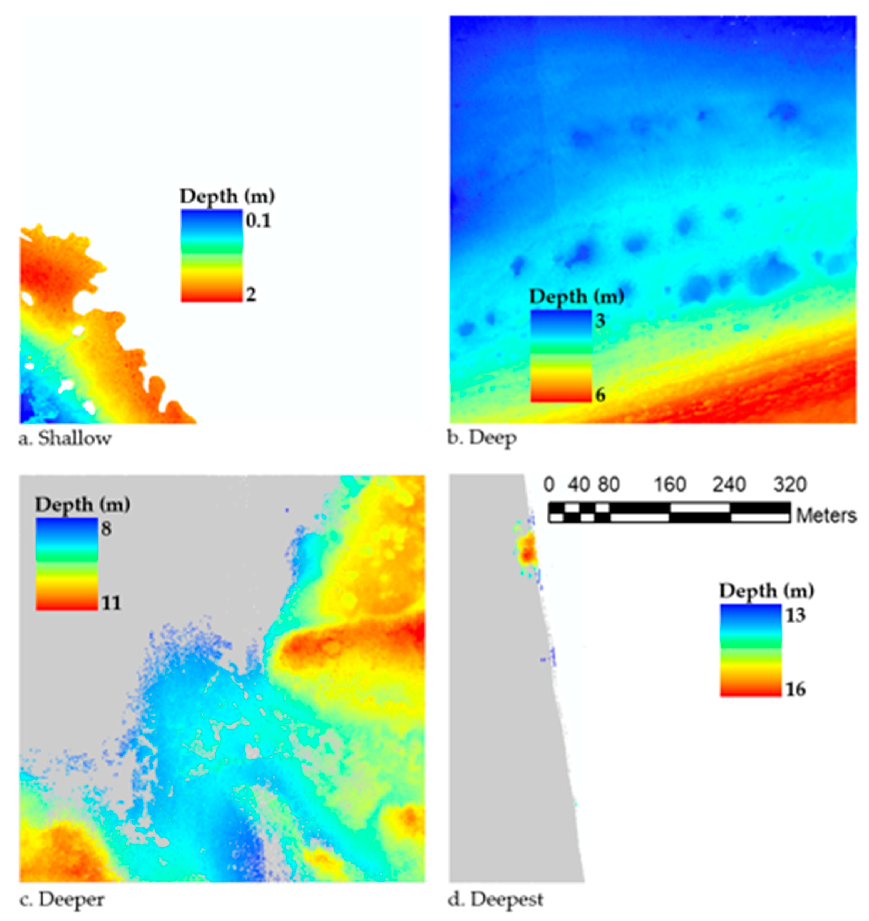
The test bed for this work comprised discrete lidar data for four 500-by-500-m CSs located in the Florida Keys (United States) in an area centered roughly on 24°35′ N latitude and 81°45′ W longitude; these were provided to the authors by NOAA. The CSs described in Table 1 and shown in Figure 3 were selected because their variability in depth, bottom surface characteristics, and data characteristics provided a representative range of conditions typically encountered operationally. For convenience, their relative depths—Shallow, Deep, Deeper, and Deepest—are used as identifiers.
Discrete lidar data for the examined CSs were acquired between 22 April and 25 April 2016, and they were provided to the authors as ‘.las’ files using the LAS data standard Version 1.4-R13 (Point Data Record Format 6) [21]. Data were acquired using a Riegel™ VQ-880-G lidar instrument that has a counter-clockwise circular scan pattern and an incidence angle of 20°. Data were acquired using an overlapping boustrophedonic (‘lawn mower’) flight pattern from an airplane flown at a nominal speed of 220 km per hour and a nominal altitude of 400 m above mean sea level (MSL); a single pass over a CS area required about 15 s.
Lidar soundings did not necessarily cover the entirety of each case study. Specifically, for the Deepest CS (Figure 3d), only two flight paths were available on the western edge. For the Shallow CS (Figure 3a), lidar data were acquired for the entire area. However, much of this CS is covered by mangrove swamps, and approximately 90% was determined by NOAA to be ‘Ground,’ i.e., above sea level. For such CSs, NOAA masks out ‘Ground’ areas and only classifies the remaining area as Bathy/NotBathy. For consistency, only the data for the area not masked out by NOAA were analyzed here.

2.2. Data

2.2.1. Predicted/Dependent Variable: Sounding Classification

The NOAA provided a Bathy/NotBathy classification of each sounding. This was produced using a combination of semi-automated procedures and human intervention. This was considered to be the most authoritative reference classification available and, in this study, was the independent variable on which ML models were fitted.

2.2.2. Predictor/Independent Variables

For analytical and discussion purposes, the predictor data were categorized as being one of three types: depth, NGSAD, or GSAD (Table 2). Each is referred to as a variable ‘suite.’

Depth

For analysis, depth was treated as its own variable ‘suite’—hence the use of ‘depth’ as data type and data nature in Table 2. Depth is expressed in meters, is negative, and is the distance from the ellipsoid height. That is, in the test bed area, MSL was approximately −21.5 m, which is the approximate distance between the ellipsoid and the geoid in the study area.

Non-Geomorphometric Sounding Attribute Data (NGSAD)

For clarity and interpretation, the variables in the NGSAD suite were further categorized by ‘type’ and ‘nature.’ The ‘sounding-specific’ NGSAD addressed the nature of each sounding. Many, e.g., intensity, scan_direct, and azim2plse, were recorded at the moment that each sounding was recorded. Others, e.g., last_of_many, were derived through NOAA post-processing. Still others, e.g., inciangle and plse_frm_hdng, were derived by the authors after a literature review suggested that additional NGSAD might contain bathymetric signal. For example, inciangle (the sensor angle of 20° corrected for yaw, pitch, and roll) was employed in lidar data processing for bathymetry in [22]. The bathymetric content of such variables has subsequently been confirmed in [23].
The ‘airplane stability’ type of NGSAD variables reflects an implicit description of instantaneous flight conditions that might relate to the bathymetric information content of soundings and be a proxy for local weather and thus turbidity conditions affecting the ocean surface and light reflectance, e.g., ocean swell direction, ocean swell height, and lidar scattering. Initially, available local weather records were explored, but it was determined that the available information lacked sufficient temporal and geographical specificity to be of use. SBET (‘Smoothed Best Estimate of Trajectory’) data are produced by the Applanix Corporation using a proprietary method based on a tightly coupled extended Kalman filter. SBET data describe the x, y, and z location of the plane and its yaw, pitch, and roll at 1/200th second intervals. SBET data also include a standard deviation for each SBET variable. These describe the certainty and temporal consistency of each SBET variable and are extracted from the Kalman filter’s post-observation covariance matrix. The standard deviations of the SBET variables were surmised to be surrogate measures of wind or ocean surface conditions (that might also impact shallow water turbidity) at the moment of pulse return acquisition. SBET uncertainties were associated with individual soundings by matching acquisition times.
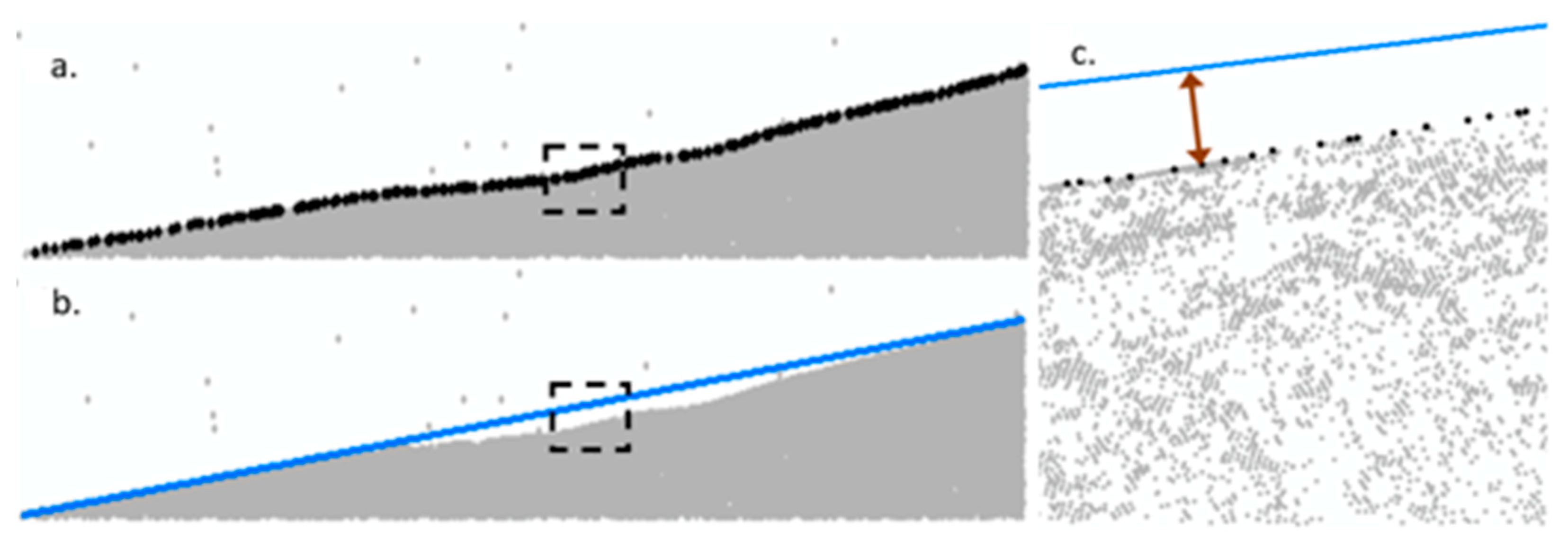
Additionally addressing flight path stability are derived ‘edge-based’ NGSAD. For each flight path on a CS, the ‘edge’ lidar soundings were identified (Figure 4a). The equation of the straight line from the ‘top corner’ to the ‘bottom corner’ of these edge soundings was derived (Figure 4b). The orthogonal deviation of each edge sounding from this straight line was then calculated (Figure 4c). These deviations were associated with individual soundings by matching acquisition times.

Geomorphometric Sounding Attribute Data (GSAD)

Geomorphometry can be derived from airborne lidar data for a range of spatial resolutions [24]. Indeed, airborne lidar is also an established technology for mapping terrestrial landforms (see, e.g., [25,26]). However, in a review article in a special issue devoted to the subject, the authors of [12] observed in 2016 that, despite growing interest, research on marine geomorphometry is less advanced. More recently, the authors [27] noted the difficulties associated with using lidar data alone to produce seamless land–sea digital elevation models (DEMs) for inter-tidal zones.
In this study, the depth (distance below the ellipsoid in m) associated with the soundings identified as Bathy by NOAA was used to derive geomorphometric characteristics over the entirety of each CS. Two types of geomorphometric information were developed: ‘Base Geomorphometry’ and ‘Orthographic Geomorphometry.’

Base Geomorphometry

The base geomorphometry variables were slope in percent and azimuthal orientation expressed in degrees. Their derivation is described by the following steps.
Step 1: Interpolate depth for the NOAA Bathy soundings on a grid within the convex hull defined by the geographic limits of the NOAA Bathy soundings.
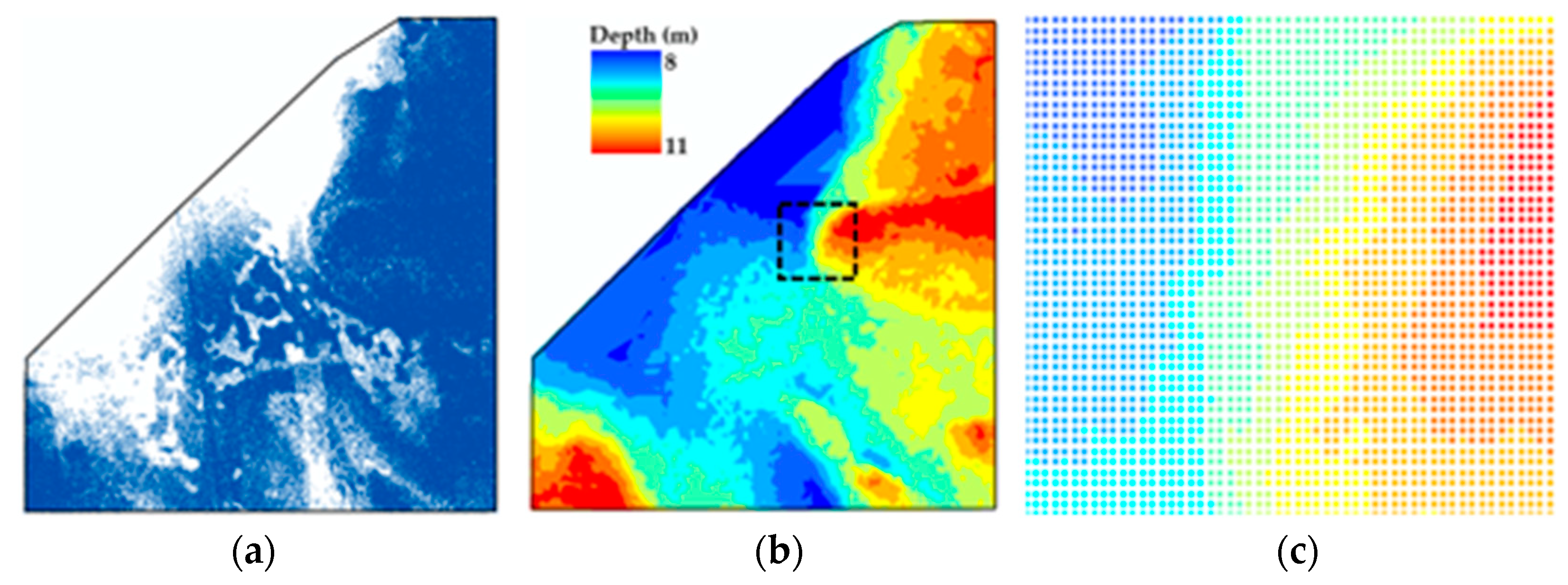
Figure 5a shows the convex hull defined by the geographic limits of the NOAA Bathy soundings for the Deeper CS. The displayed convex hull was in fact 5 m inside the geographic limits of the NOAA Bathy soundings; this 5 m buffer is required for a number of operations such as ensuring that slope maps do not treat data edges as being areas of abrupt depth changes. TIN (triangular irregular network)-based linear interpolation was applied to the depth associated with the NOAA Bathy soundings to interpolate depth to a grid within the convex hull (Figure 5b,c). This interpolation provided a depth estimate for every point within the convex hull. It made the implicit assumption that the slope between any two points was a plane. Though reasonable over short distances, it became less reasonable as the length of sides of individual triangles comprising the TIN increased and triangles became less equilateral. Once produced, the TIN was converted to separate spatially regular 1 and 5 m grids, which were both employed to enable the consideration of fine-scale and coarser-scale geomorphometry.
Step 2: Extrapolate depths to points beyond geographical limits of known Bathy soundings.
A set of ‘exterior points’ was established around the edges of the entire CS at a 15 m spacing (Figure 6a)—a spacing that was subjectively evaluated as being broadly suitable. Conceptually, the bathymetry-bounding grid points developed in Step 1 were used to extrapolate depth along a plane to each of the exterior points; grid points depths considered to be anomalous or highly uncertain were removed. The validity of doing this relied on the implicit assumption that the geomorphometry at the limits of known data was indicative of the geomorphometry beyond, e.g., slope, aspect, and rugosity were all similar on both sides of the convex hull. Operationally, for each of the exterior points, a 4 m-wide polygon (Figure 6b) from the geometric center of the convex hull was established, and the grid points (Figure 5c) within 10 meters of the convex hull that were closest to each of the exterior points were extracted (Figure 6c); 4 and 10 m were subjectively judged to provide a sufficient but not excessive number of points for extrapolation for a range of spatial configurations.
For each exterior point, a linear regression was fitted to the grid points extracted by the 4 m-wide polygon. Its form is:
Z = a + bX + cY
where Z is the depth in meters; X and Y are Universal Transverse Mercator (UTM) coordinates; and a, b, and c are regression coefficients. The X–Y coordinates of the subject exterior point were used in the regression equation to estimate its depth. Exterior points were eliminated from further analysis if their regression line had a root-mean-square-error (RMSE) greater than 1 cm, there were fewer than 15 points available for model fitting, or the R2 of the regression line was less than 0.75. The Deeper CS used for illustration in Figure 5 and Figure 6 was representative of the varying certainty of the extrapolated depth of exterior points related to the spatial distribution of known bathymetry soundings. That is, where NOAA Bathy soundings extended to the edge of the CS (the south and east in Figure 6a), the distance over which depth was extrapolated was small and certainty likely to be higher than for exterior points for which the extrapolation distance was large (e.g., the northwest of Figure 6a).
Step 3: Interpolate depths on a whole-of-CS point grid using the known Bathy soundings and the extrapolated depths of the exterior points. Convert point grid to a raster. Determine slope and orientation.
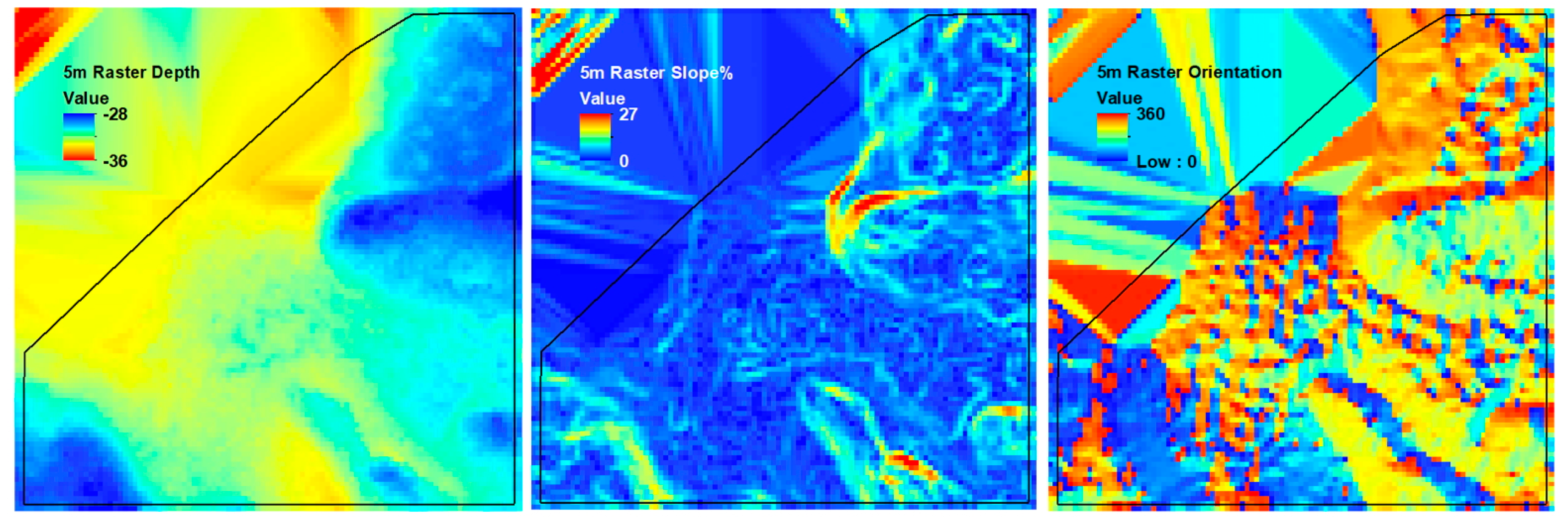
A grid of points of user-specified spacing—1 and 5 m in this study—was established across the CS limits to the exterior extrapolated points. The depth of each grid point was determined via distance-weighted linear interpolation using the depths of the NOAA Bathy soundings and the exterior points whose depths were extrapolated. This depth grid was then converted to a raster of the same resolution as the grid, and the slope in percent and azimuthal orientation were obtained using a 3-by-3 raster window around each raster cell (Figure 7). Slope and orientation rasters were then clipped to the geographic limits of the CS. Note that extrapolated depth was solely employed to produce the slope and orientation surfaces; in the subsequently fitted ML models, it was the depth associated with each sounding that was employed.
The impact of this ‘plane fitting extrapolation method’ for slope and orientation using sparse or absent Bathy data is readily apparent in Figure 7. For the Deeper CS, the slope and orientation maps were understandably more regular in the highly extrapolated northwest than the southeast, where Bathy data were abundant. Though the GSAD in the northwest were cartographically and analytically most uncertain, such data represented the best geomorphometric information that could be produced using the employed method.
After applying this method to all four CSs, the slope and orientation for each lidar sounding were extracted using spatial overlay. Because the developed method was applied using 1 and 5 m grids, base geomorphic variables were subsequently referred to using slopepct_ or orient_ as prefixes denoting interpolated slope or orientation, and 1 or 5 m were added as suffixes to denote grid resolution, e.g., orient_1 m refers to the orientation derived from the use of a 1 m grid.

Orthographic Geomorphometry

Orthographic geomorphometry—a second type of GSAD—relates the orientation and slope to the incident scan angle (inciangle) and azimuthal direction of the pulse (azim2plse) that generated the sounding. The employed approach was conceptually comparable to Lambertian reflectance [28]. Separate orthogonality indices were calculated for orientation and slope. The calculation of each could best be illustrated using an example: a pulse generated due east (i.e., azim2plse of 90°) with an inciangle of 20°.
Orientation orthogonality, Ψ, 0 ≤ Ψ ≤ 100, is calculated:
Ψ = 100 ½(1-cos∣ф − θ∣)
where ф is azim2plse and θ is orientation.
Slope orthogonality, Θ, is dependent on whether slope orientation is towards or away from the origin of the lidar pulse (the airplane). Moreover, maximum reflectance (and orthogonality) results from a pulse that strikes the ocean floor where the slope is equal to the inciangle and has an orientation exactly opposed to the azim2plse. Thus, for soundings whose orientation is towards the plane, i.e., azim2plse is not within 90° of the orientation, Θ is calculated:
Q ^ = 100 cos2(∣Ф + φ∣)
where ф is inciangle and φ is slope. For soundings whose slope φ is oriented away from the airplane, i.e., azim2plse is within 90° of the orientation, slope orthogonality Θ is calculated:
Q ^ = 100 cos2(∣Ф − φ∣)
Though theoretically, 0 ≤ Θ ≤ 100, the observed range was 40 ≤ Θ ≤ 100.
Orthogonal geomorphic variables are subsequently referred to using ori_orthog_ or slp_orthog_ as prefixes denoting orientation or slope orthogonality and 1 or 5 m as a suffix denoting grid resolution, e.g., ori_orthog_1 m.

2.3. Modelling and Analysis

2.3.1. Model Fitting

Models to predict/classify the binary NOAA Bathy/NotBathy classification were fitted using extreme gradient boosting (XGB) [29] with lasso (‘11′) regularization applied. Additionally and initially examined for this binary classificatory modelling were regularized logistic regression and multilayer perceptrons—a form of neural network; XGB outperformed both techniques in accuracy and speed, and it was retained for use. XGB is based on the principles of gradient boosting [30], but XGB is less prone to over-fitting because of its inherently more regularized model structure. XGB is a tree-based machine learning (ML) technique that ‘grows’ a series of shallow classification trees. Each successive tree is produced by focusing classification improvement on the soundings with the largest prediction errors. The final model was produced using a majority-weighted ‘vote.’ Lasso regularization added a penalty to the XGB cost-function that resulted in the impact of ‘unimportant’ variables being driven to zero (0).
For each CS, XGB models were fitted for each of the three variable suites—depth, NGSAD, and GSAD—individually, the three two-way combinations, and the single three-way combination. Models were fitted after normalizing all independent variables between 0 and 100 using CS-specific maximums and minimums. The model containing depth alone was considered the ‘null’ or ‘base’ model because of depth’s clear relationship with bathymetry. Comparing its goodness-of-fit statistics with those of the other six models provided a means to compare the bathymetric signal in depth against the NGSAD of GSAD alone, and to evaluate the marginal contribution or signal strength of NGSAD and GSAD in models containing depth.
The XGB models estimated the probability that each sounding was bathymetry, i.e., p(Bathy). To conventionally evaluate model accuracy, model-based probabilities were classified using a probability decision threshold (PDT) of 0.50. That is, any sounding for which p(Bathy) was 0.50 or greater was classified as Bathy; all others were classified as NotBathy. However, because ML models globally optimize cost functions, cost functions of classification models can maximize global accuracy. This could result in the accuracy of the majority class being improved at the expense of the accuracy of the minority class. This was observed to varying degrees in all CSs in this study: Bathy was a strong majority for the Shallow CS (78% of total soundings) and Deep CS (76%) and strong minority for the Deeper CS (21%) and the Deepest CS (0.4%) (Row 8, Table 1). The impact of not adjusting for globally optimized models was most apparent for the Deepest CS. Applying a PDT of 0.50 to probabilities from a globally optimized model where only 0.4% (3902 of one million observations) were Bathy produced a very high yet meaningless global accuracy of 99.6%. That is, even without a model, classifying 100% of soundings as the heavily dominant NotBathy class produced a classification that was 99.6% globally accurate, but that had little value for bathymetric mapping.
To mitigate the impact of ‘imbalanced’ dependent variables, weighting, re-sampling, and an alternative PDT were examined. Inverse proportional weighting entailed weighting the prediction error on each Bathy sounding by the inverse proportion of Bathy pulse returns in the data. Re-sampling imputed a sufficient number of additional minority class ‘pseudo-soundings’ to overcome the class imbalance prior to model fitting. Two types of re-sampling were evaluated: SMOTE (Synthetic Minority Oversampling Technique) [31] and ADASYN (Adaptive Synthetic Sampling Approach) [32]. The third alternative—the use of a PDT different from 0.50—performed the best and was subsequently employed. Hence, further explanation is provided.

2.3.2. Model Evaluation (Depth, NGSAD, and GSAD Assessment)

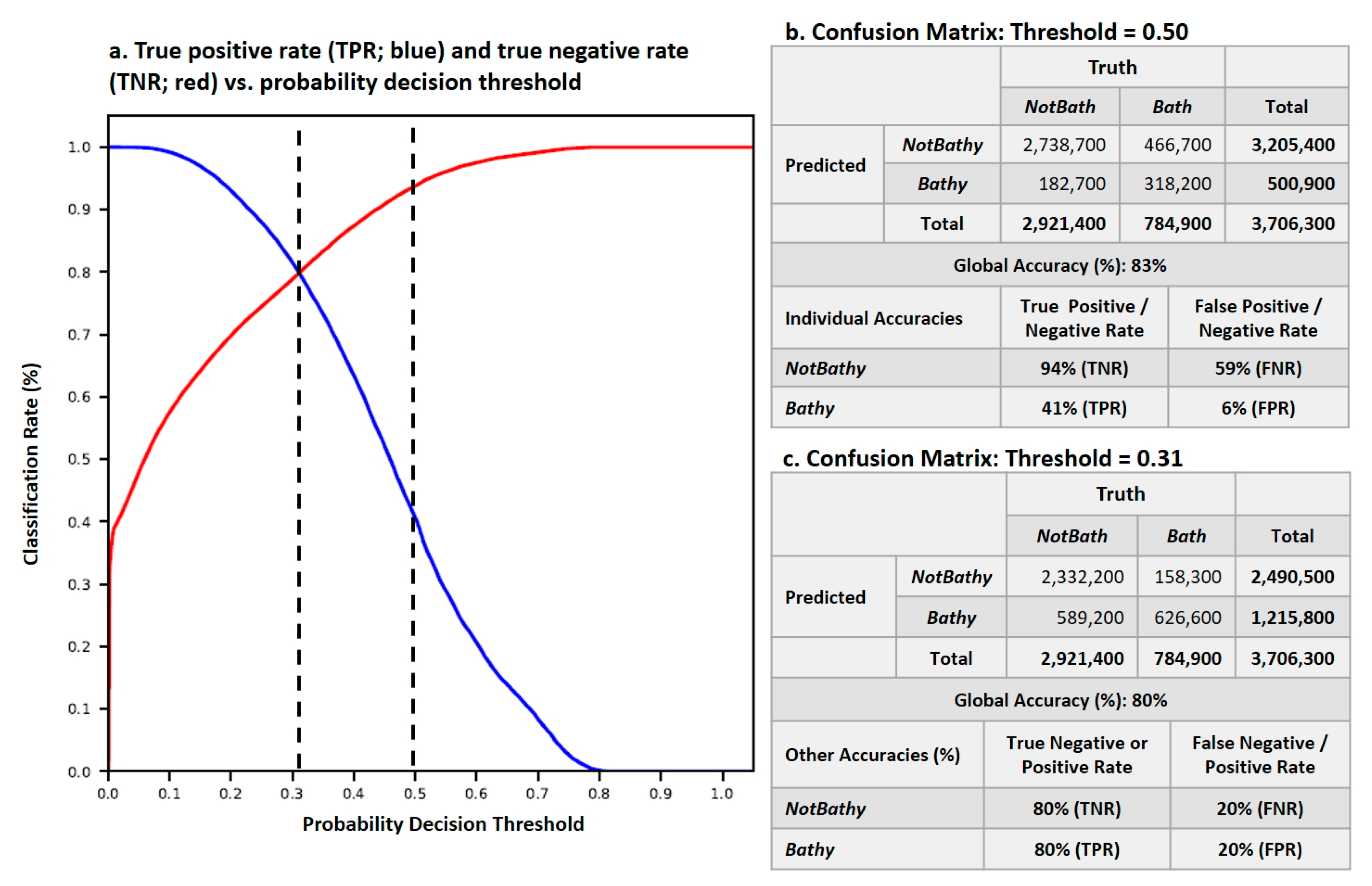
Models fitted on CSs like the Deepest where bathymetry was ‘rare’ resulted in the p(Bathy) of relatively few soundings exceeding 0.50. Thus the use of the conventional PDT of 0.50 caused a relatively low true positive (Bathy) rate (TPR) compared to a much higher true negative (NotBathy) rate (TNR). This is apparent in Figure 8b and also demonstrated in Figure 8a where the TPR (blue line) is much lower than the TNR (red line) when the PDT was 0.50. The point at which the TPR and TNR intersected—0.31 in Figure 8a—is termed the “Optimal Decision Threshold” (ODT) here. Though its application to p(Bathy) decreased global accuracy from 83% to 80% (Figure 8b,c), the ODT increased the TPR from 41% to 80%. Of particular interest was that the use of the ODT caused the number of false negatives (FNs, i.e., undetected Bathy), which are potentially the most serious errors for bathymetric chart users, to decrease by about two-thirds (from 466,700 to 158,300), thus resulting in a decrease in FNR from 59% to 20%.
The ODT was used in all subsequent model evaluations. For each model, soundings were assigned to Bathy or NotBathy based on their p(Bathy) values estimated by an XGB model. The soundings were then cross-tabulated by their NOAA and XGB Bathy/NotBathy classifications, and the following summary statistics were calculated: global accuracy, TNR, FNR, TPR, and FPR. Note that in a practical sense, it is the FN errors that are most critical to marine safety and navigation.

2.3.3. Individual Variable Evaluation

As a final step, the ‘importance’ of individual variables containing depth and the NGSAD variable suite was examined; models that included the GSAD variable suite were not examined because of its weak predictive ability, as will be shown, indicating low bathymetric signal strength. The XGB model-fitting provided a measure of the ‘importance’—but not statistical significance—of each variable. Importance is the percent of the multiple shallow trees/models in which a variable appears, normalized over all variables so that the sum of importance over all variables equals 100. For each CS, the five most important variables for the ‘depth and NGSAD’ model were identified, their cumulative importance was calculated, the number of variables whose importance was greater than 0.0 was noted, and the variables whose importance was zero were identified.

3. Results

3.1. Model Evaluation (Depth, NGSAD, and GSAD Assessment

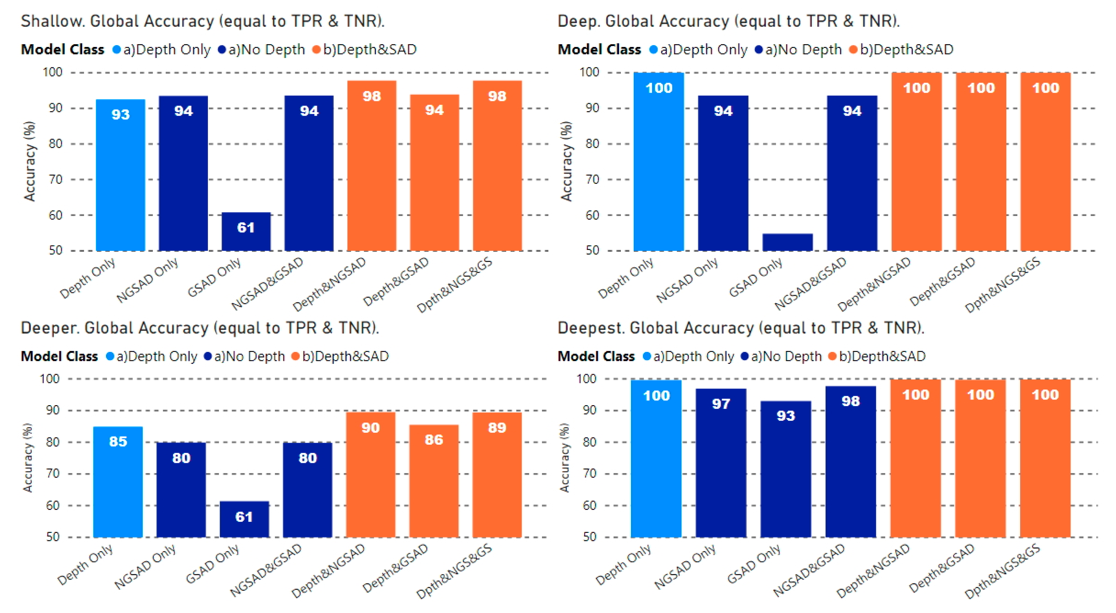
(Pseudo) R2 values (McFadden’s pseudo R2 for classification [33], which cannot be tested for statistical significance) (Figure 9) confirmed that depth was highly related to bathymetry. Less expected was that models fitted on the NGSAD variable suite alone produced comparable R2 values. Even for the Deeper CS, for which models performed the most poorly, R2 values were approximately 0.35 for models containing the NGSAD variable suite alone. Given that a conventional R2 value of 0.35 for >100,000 observations was statistically significant, these results suggested that a strong bathymetric signal was present in the NGSAD variable suite alone.
Except for the Deep CS, the pseudo R2 values indicated that the best models were comprised of depth and the NGSAD variable suite. The Deep CS had a relatively simple geomorphometry and depths that were optimal for airborne lidar; in such conditions, depth alone appeared to be sufficient to accurately classify Bathy/NotBathy soundings. For the Shallow CS, a large percentage (72%) of soundings were classified by NOAA as Bathy, but depth alone did not produce the model with the highest pseudo R2. In shallow areas such as the Shallow CS, the vertical noise in the lidar point cloud could be larger than the ocean depth and depth alone were not sufficient for accurate sounding classification. NGSAD variables enhanced bathymetry extraction in shallow areas, as well as in areas near the limit of lidar penetration (the Deeper and Deepest CSs).
The model classification accuracy/error rates (Figure 10 and Figure 11) reinforced the conclusions of the pseudo R2 values about model strength and the importance of different variable suites:
  • The GSAD variable suite had the lowest predictive ability for bathymetry on its own (‘GSAD only’ models) and provided little or no additional marginal benefit when incorporated into models with depth and/or the NGSAD variable suite.
  • Depth was consistently the strongest stand-alone indicator of bathymetry. However, in shallow areas, the bathymetric signal strength in the NGSAD variable suite alone was comparable to the signal strength in depth alone. Nonetheless, in shallow areas, it was the combination of depth and the NGSAD variable suite that provided the best bathymetry extraction.
  • The models with the greatest bathymetry predictive power and that were most efficient, i.e., fewest variables for a given accuracy, were the models that employed depth and the NGSAD variable suite.

3.2. Individual Variable Evaluation

It was determined that the GSAD variables did not contribute to model improvement as well as depth alone, NGSAD variables alone, or the combination of depth and NGSAD variables. Unsurprisingly, therefore, no GSAD variable of either spatial resolution (1 or 5 m) was among the five most important variables for any model that consistently represented at least 80% of variable importance (Table 3). Because of the very minor contribution of GSAD variables, their individual importance was not further considered.
While depth was consistently the most important variable in each model (Column 4, Table 3), the NGSAD suite enhanced the classification accuracy of XGB models for all CSs:
  • At least 10 variables were important in all models (Column 2, Table 3)
  • NGSAD were—along with depth—consistently among the five most important variables (Column 4, Table 3), which had a combined importance of at least 0.80 (or 80% of the total; Column 5, Table 3).
The following are notable points about the presence of specific variables in a given model are notable (Column 4, Table 3):
  • Last was the second most important variable in the Shallow, Deeper, and Deepest CSs; further analyses indicated that not being the first (sounding) return from a lidar pulse increased p(Bathy).
  • SBET variables (particularly stdXYZ) describing airplane/platform stability—and therefore presumably local wind and surface reflectance characteristics—were among the five most important variables in all models.
  • The presence of azim2pls in models for two CSs (Deep and Deepest) may also have captured a bathymetric signal related to momentary surface or ocean conditions since there was no instrumental or other reason that a particular azimuth would be better or worse for identifying bathymetry.
  • Inciangle (the 20° instrument angle corrected for yaw, pitch, and roll) was important for all CSs except the Deepest CS; this may also relate to how the dynamics of light reflection and/or penetration relate to bathymetry in lidar data.
  • Surprisingly, intensity was only among the five most important variables for two CSs, suggesting that other NGSAD related more to the bathymetric signal of soundings.
Regarding GSAD variables not improving XGB models nor being among the five most important variables for any case study, it was notable that two spatial resolutions—1 and 5 m—were considered. Hence, even the consideration of multiple spatial resolutions did not provide geomorphometric information that is useful for identifying bathymetry.

4. Discussion

It is well-established that the energy return from active sensors is impacted by ocean bottom characteristics in ocean mapping (e.g., [8,9,10,11,34]). Hence, the failure of geomorphometry/GSAD variables to improve XGB models containing depth and NGSAD variables demonstrated that procedures used herein to derive GSAD variables were ineffective at two spatial resolutions—1 and 5 m—for the purposes of improving extraction of bathymetric soundings from lidar point clouds under the studied conditions. This was most understandable for the Deeper and Deepest CSs (Figure 3c,d) that were subject to extensive extrapolation due to lack of lidar penetration and Bathy soundings across the entire CS. However, it was also true of the Shallow and Deep CSs (Figure 3a,b), where interpolation rather than extrapolation was the dominant process due to the availability of Bathy soundings across the entire CS. The further study of the error structure might indicate a minimum density of Bathy soundings required to extract useful GSAD. Nonetheless, the inability to produce useful geomorphometry variables even for the CSs—Shallow and Deep—with spatially complete Bathy coverage suggested that methods other than those employed here would need to be developed.
A potentially important factor to consider in any future work is the directionality of geomorphometry relative to the flightpath direction. In this study, the variables scan_direct (forward or backward scan) and azim2pls (azimuth of a pulse) may have been able to implicitly characterize this relationship. Indeed, azim2pls, being one of the five most important variables for the Deep and Deepest CSs, may reflect this. However, the overlap between adjacent north-to-south and south-to-north flight paths would likely have obscured any such relationship that might have been present. Explicitly examining this relationship may improve the ability to separate Bathy soundings from NotBathy soundings.
Regardless of how future work in this area might be approached, spatial scale is a consideration in two major ways. The first is the footprint of laser pulses when they strike the ocean floor. When a lidar pulse strikes the ocean surface, it increasingly expands in diameter with increasing ocean depth. Thus, it is possible that the scale at which geomorphometry would need to be characterized would change with depth. Further, the reality that a large-footprint lidar pulse would reflect differently than a small-footprint lidar pulse adds considerable complexity to the problem. The second is that the suitability of any geomorphometry-inclusive analysis for identifying bathymetry is highly dependent on the targeted application. In this study, the intended application was the production of highly accurate and precise nautical charts—an output requiring very high-quality information. For other applications, however, data requirements might not be as rigorous. One can imagine that in mapping, e.g., a benthic habitat, kelp beds, or aquatic species that are not threatened or endangered, one would be able to relax data standards. Perhaps useful methods of extracting geomorphometry from lidar point clouds that would be sufficiently accurate for such purposes could be developed. Similarly, application domains that are heavily impacted by shallow water geomorphometry but for which there is currently a near-complete lack of geomorphometry information may find that the described methods provide a characterization of geomorphometry that, though clearly inexact, represents an improvement on existing knowledge that has application-specific utility.
A key underlying assumption of spatial interpolation and extrapolation is that the characteristics of geomorphometry as one approaches spatial data limits continue and are indicative of geomorphometry beyond the spatial data limits. The inability of the methods examined here to describe geomorphometry in a way that is useful for extracting bathymetry from lidar point clouds where data are sparse or non-existent suggests this was not true that in the examined area and ocean conditions. One solution to overcoming this may be a judicious use of optical imagery. For example, the authors of [35] used World View 2 imagery to address gaps in bathymetry obtained using sonar data up to a depth of 35 m, i.e., beyond the limits of lidar penetration. Such a data integration approach might prove useful for lidar-based shallow water bathymetry and geomorphometry.
The successful development of such a “data fusion” approach would be a worthwhile pursuit for the remote sensing research community. In bathymetric mapping, shallow areas are generally of the greatest interest because of their proximity to human activities but also present the greatest challenges. Establishing remote sensing-based methods that merge lidar data covering depths from 0 to approximately 20 m with optical data that address depths to 35 m or so would address a considerable gap in hydrographic mapping.

5. Conclusions

A strong bathymetric signal can be extracted from airborne lidar soundings for shallow water (<17 m) by using a sounding’s depth and non-geomorphometric sounding attribute data. The explanatory power of individual variables is dispersed over factors that describe individual sounding characteristics and factors associated with the stability of the airborne platform at the instant of return acquisition. Geomorphometric data that were derived using spatial extrapolation and interpolation only had a weak relationship with bathymetric signal regardless of water depth. Notably, geomorphometric variables had been considered at two spatial scales (1 and 5 m), but neither improved the identification of soundings that were bathymetry. That the relationship between geomorphometry and light reflectance is well-established was noted in the introduction. Hence the inability to employ this relationship to improve bathymetric extraction demonstrates the difficulty of obtaining meaningful spatially complete geomorphometric descriptors in areas where bathymetric data are locally sparse or non-existent. This may also be related to the size of a lidar pulse footprint when it strikes the ocean floor, which varies with depth. It may also be due to directionality of the geomorphometry relative to the flight path that was not considered in this study.

Author Contributions

Conceptualization: K.L. and B.C.; methodology: K.L.; software: K.L. and B.C.; validation: K.L.; formal analysis: K.L.; writing—original draft preparation: K.L.; writing—review and editing: K.L. and B.C. All authors have read and agreed to the published version of the manuscript.

Funding

This work was supported by the National Oceanic and Atmospheric Administration (NOAA) under Grant NA15NOS400020.

Data Availability Statement

The data that support the findings of this study are available at the link https://figshare.com/s/b72248f6e02f58f299a4 (accessed on 16 February 2021). SBET data in the required format are provided at the figshare link. Though the last data used are available to the public, the authors are not authorized to make them directly available; a small sample of the data for a single data CS are provided at the figshare link to demonstrate format. Effective 15 March 2017 (2017-03-15) complete data sets (2016_420500e_2728500n.laz, 2016_426000e_2708000n.laz, 2016_428000e_2719500n.laz, and 2016_430000e_2707500n.laz) can be downloaded from https://coast.noaa.gov/digitalcoast/data/ (accessed on 16 February 2021) (Data set name: “2016 NGS Topobathy Lidar: Key West FL”) as compressed laz files. These can be decompressed using the LASzip tool which can be downloaded from laszip.org.

Conflicts of Interest

The authors declare no conflict of interest.

Abbreviations

AcronymDefinition
ADASYNAdaptive Synthetic Sampling Approach
CHRTCUBE with Hierarchical Resolution Techniques
CSCase Study
ENEstimation Node
FNR/FPRFalse Negative/Positive Rate
GSADGeomorphometric Sounding Attribute Data
LASNot an acronym; a file containing lidar data
MBESMulti-Beam Echo Sounder
MLMachine Learning
MSLMean Sea Level
NOAANational Oceanic and Atmospheric Administration (United States)
NGSADNon-Geomorphometric Sounding Attribute Data
ODTOptimal Decision Threshold
P(Bathy)Probability of an individual sounding being Bathy
PDTProbability Decision Threshold
RMSERoot mean square error
SADSounding Attribute Data
SMOTESynthetic Minority Oversampling Technique
TINTriangulated Irregular Network
TNR/TPRTrue Negative/Positive Rate
UTMUniversal Transverse Mercator
XGBExtreme Gradient Boosting

References

  1. Allouis, T.; Bailly, J.-S.; Pastol, Y.; Le Roux, C. Comparison of LiDAR waveform processing methods for very shallow water bathymetry using Raman, near-infrared and green signals. Earth Surf. Process. Landf. 2010, 35, 640–650. [Google Scholar] [CrossRef]
  2. Dix, M.; Abd-Elrahman, A.; Dewitt, B.; Nash, L., Jr. Accuracy evaluation of terrestrial LIDAR and multibeam sonar systems mounted on a survey vessel. J. Surv. Eng. 2012, 138, 203–213. [Google Scholar] [CrossRef]
  3. Calder, B.; Mayer, L. Automatic processing of high-rate, high-density multibeam echosounder data. Geochem. Geophys. Geosystems 2003, 4, 22. [Google Scholar] [CrossRef]
  4. Calder, B.; Rice, G. Computationally efficient variable resolution depth estimation. Comput. Geosci. 2017, 106, 49–59. [Google Scholar] [CrossRef]
  5. Fischler, M.; Bolles, J. Random sample consensus—A paradigm for model fitting with applications to image analysis and automated cartography. Commun. ACM 1981, 24, 381–395. [Google Scholar] [CrossRef]
  6. Nayegandhi, A.; Brock, J.; Wright, C. Small-footprint, waveform-resolving lidar estimation of submerged and sub-canopy topography in coastal environments. Int. J. Remote Sens. 2009, 30, 861–878. [Google Scholar] [CrossRef]
  7. Nagle, D.; Wright, C. Algorithms Used in the Airborne Lidar Processing System (ALPS); Dept. of the Interior/U.S. Geological Survey Open File Report 2016–1046; United States Geological Survey: Reston, VA, USA, 2016; p. 45.
  8. Pe’eri, S.; Gardner, J.; Ward, L.; Morrison, J. The seafloor: A key factor in lidar bottom detection. IEEE Trans. Geosci. Remote Sens. 2011, 49, 1150–1157. [Google Scholar] [CrossRef]
  9. Niroumand-Jadidi, M.; Vitti, A.; Lyzenga, D. Multiple optimal depth predictors analysis (MODPA) for river bathymetry: Findings from spectroradiometry, simulations, and satellite imagery. Remote Sens. Environ. 2018, 218, 132–147. [Google Scholar] [CrossRef]
  10. Collin, A.; Archambault, P.; Long, B. Mapping shallow water seabed habitat with the SHOALS. IEEE Trans. Geosci. Remote Sens. 2008, 46, 2947–2955. [Google Scholar] [CrossRef]
  11. Wedding, L.; Friedlander, A.; McGranaghan, M.; Yost, R.; Monaco, M. Using bathymetric lidar to define nearshore benthic habitat complexity: Implications for management of reef fish assemblages in Hawaii. Remote Sens. Environ. 2008, 112, 4159–4165. [Google Scholar] [CrossRef]
  12. Lecours, V.; Dolan, M.; Micallef, A.; Lucieer, V. A review of marine geomorphometry, the quantitative study of the sea floor. Hydrol. Earth Syst. Sci. 2016, 20, 3207–3244. [Google Scholar] [CrossRef] [Green Version]
  13. White, M.; Mohn, C.; Orren, M. Physical processes and seamount productivity. In Seamounts: Ecology, Fisheries and Conservation; Blackwell Publishing: Oxford, UK, 2007; pp. 65–84. [Google Scholar]
  14. Kunze, E.; Llewellyn Smith, S. The role of small-scale topography in turbulent mixing of the global ocean. Oceanography 2004, 17, 55–64. [Google Scholar] [CrossRef]
  15. McArthur, M.; Brooke, B.; Przeslawski, R.; Ryan, D.; Lucieer, V.; Nichol, S.; McCallum, A.; Mellin, C.; Cresswell, I.; Radke, L. On the use of abiotic surrogates to describe marine benthic biodiversity. Estuar. Coast. Shelf Sci. 2010, 88, 21–32. [Google Scholar] [CrossRef]
  16. Eren, F.; Pe’eri, S.; Rzhanov, Y.; Ward, L. Bottom characterization by using airborne lidar bathymetry (ALB) waveform feature obtained from bottom return residual analysis. Remote Sens. Environ. 2018, 206, 260–274. [Google Scholar] [CrossRef]
  17. Wang, C.-K.; Philpot, W. Using airborne bathymetric lidar to detect bottom type variation in shallow waters. Remote Sens. Environ. 2007, 106, 123–135. [Google Scholar] [CrossRef]
  18. Wang, C.; Li, Q.; Liu, Y.; Wu, G.; Liu, P.; Ding, X. A comparison of waveform processing algorithms for single-wavelength LiDAR bathymetry. Isprs J. Photogramm. Remote Sens. 2015, 101, 22–35. [Google Scholar] [CrossRef]
  19. Lucieer, V.; Lecours, V.; Dolan, M. Charting the course for future developments in marine geomorphometry: An introduction to the special issue. Geosciences 2018, 8, 477. [Google Scholar] [CrossRef] [Green Version]
  20. Tulldahl, H.; Wikström, S. Classification of aquatic macrovegetation and substrates with airborne lidar. Remote Sens. Environ. 2012, 121, 347–357. [Google Scholar] [CrossRef]
  21. American Society for Photogrammetry and Remote Sensing. Las Specification Version 1.4-R13; American Society for Photogrammetry and Remote Sensing: Bethesda, MD, USA, 2013; pp. 15–18. [Google Scholar]
  22. Fernandez-Diaz, F.; Glennie, C.; Carter, W.; Shrestha, R.; Sartori, M.; Singhania, A.; Legleiter, C.; Overstreet, B. Early results of simultaneous terrain and shallow water bathymetry mapping using a single-wavelength airborne LiDAR sensor. IEEE J. Sel. Top. Appl. Earth Obs. Remote Sens. 2014, 7, 623–635. [Google Scholar] [CrossRef]
  23. Lowell, K.; Calder, B. Measuring shallow-water bathymetric signal strength in lidar point attribute data using machine learning. Int. J. Geogr. Inf. Sci. 2020, in press. [Google Scholar] [CrossRef]
  24. Pittman, S.; Costa, B.; Battista, T. Using lidar bathymetry and boosted regression trees to predict the diversity and abundance of fish and corals. J. Coast. Res. 2009, 53, 27–38. [Google Scholar] [CrossRef]
  25. Höfle, B.; Rutzinger, M. Topographic airborne LiDAR in geomorphology: A technological perspective. Z. Geomorphol. 2011, 55, 1–29. (In English) [Google Scholar] [CrossRef]
  26. Sarala, P.; Räisänen, J.; Johansson, P.; Eskola, K. Aerial LiDAR analysis in geomorphological mapping and geochronological determination of surficial deposits in the Sodankylä region, northern Finland. GFF 2015, 137, 293–303. [Google Scholar] [CrossRef]
  27. Andersen, M.; Gergely, A.; Al-Hamdani, Z.; Steinbacher, F.; Larsen, L.; Ernstsen, V. Processing and performance of topobathymetric lidar data for geomorphometric and morphological classification in a high-energy tidal environment. Hydrol. Earth Syst. Sci. 2017, 21, 43–63. [Google Scholar] [CrossRef] [Green Version]
  28. Koppal, S. Lambertian reflectance. Encyclopedia of Computer Vision; Katsushi, I., Ed.; Springer: London, UK, 2014; pp. 441–443. [Google Scholar]
  29. Chen, T.; Guestrin, C. XGBoost: A scalable tree boosting system. In Proceedings of the 22nd ACM SIGKDD International Conference on Knowledge Discovery and Data Mining (KDD ’16), San Francisco, CA, USA, 13–17 August 2016; pp. 785–794. [Google Scholar] [CrossRef] [Green Version]
  30. Friedman, J. Greedy function approximation: A gradient boosting machine (1999 Reitz Lecture). Ann. Stat. 2001, 29, 1189–1232. [Google Scholar] [CrossRef]
  31. Chawla, N.; Bowyer, K.; Hall, L.; Kegelmeyer, W. SMOTE: Synthetic minority over-sampling technique. J. Artif. Intell. Res. 2002, 16, 321–357. [Google Scholar] [CrossRef]
  32. He, H.; Bai, Y.; Garcia, E.; Li, S. ADASYN: Adaptive synthetic sampling approach for imbalanced learning. In Proceedings of the IEEE International Joint Conference on Neural Networks (IJCNN 2008), Hong Kong, China, 1–8 June 2008; pp. 1322–1328. [Google Scholar] [CrossRef] [Green Version]
  33. McFadden, D. Conditional logit analysis of qualitative choice behavior. In Frontiers in Econometrics; Zarembka, P., Ed.; Academic Press: Cambridge, UK, 1974; pp. 105–142. [Google Scholar]
  34. Measures, R. Laser Remote Sensing: Fundamentals and Applications; Krieger: Melbourne, FL, USA, 1992; p. 510. [Google Scholar]
  35. Linklater, M.; Hamylton, S.; Brooke, B.; Nichol, S.; Jordan, A.; Woodroffe, C. Development of a Seamless, High-Resolution Bathymetric Model to Compare Reef Morphology around the Subtropical Island Shelves of Lord Howe Island and Balls Pyramid, Southwest Pacific Ocean. Geosciences 2018, 8, 11. [Google Scholar] [CrossRef] [Green Version]
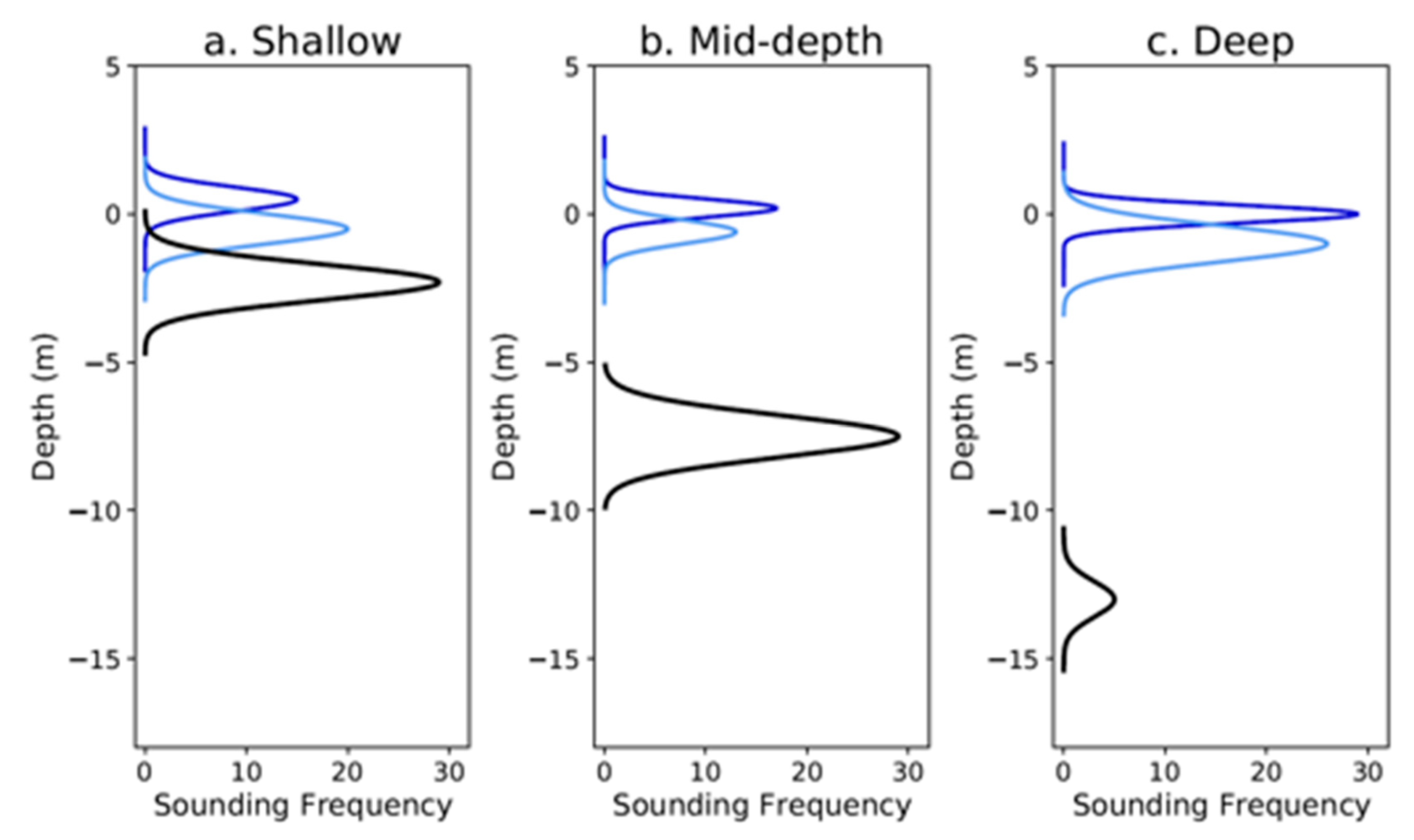
Figure 1. Representative sounding frequency distributions for hypotheses for individual estimation nodes (ENs) representing three depths. (ac) depict representative hypotheses for, respectively, shallow, mid-depth, and deep areas. The blue hypotheses represent the ocean surface, and the black hypotheses are the (correct) ocean floor hypotheses.
Remotesensing 13 01604 g001
Figure 2. Schematic flow of data preparation and model development and evaluation. (GSAD: geomorphometric sounding attribute data; NGSAD: Non-geomorphometric sounding attribute data); SBET: smoothed best estimate trajectory).
Remotesensing 13 01604 g002
Figure 3. Map of ocean depth for the four CS areas; mean depth is presented for 1 m pixels of Bathy soundings. (ad) show CSs used for methodology development ordered from shallowest (a) to deepest (d). Only gray and colored areas have usable data; white areas either have no soundings due to flight path or soundings judged to be above MSL. Gray areas contain only NotBathy soundings.
Remotesensing 13 01604 g003
Figure 4. Extraction of deviations from a straight flight path. (a) Lidar sounding cloud (gray) and derived edge soundings (black). The dashed box is the area of enlargement in (c). (b) Edge corner-to-corner straight flight path (blue line). (c) Orthogonal deviation (brown arrow) of a single edge sounding from the corner-to-corner flight path edge of lidar sounding cloud.
Remotesensing 13 01604 g004
Figure 5. Example of steps in obtaining geomorphometric characteristics for an entire CS (Deeper). ((a) left) The NOAA Bathy soundings in blue and the associated convex hull. ((b) center) The interpolated 5 m grid of points and the area of enlargement in (c).
Remotesensing 13 01604 g005
Figure 6. Extrapolation to points beyond the CS edge. ((a) left) The NOAA Bathy soundings and regularly spaced ‘exterior points’ beyond the CS limits. ((b) center) A 4 m-wide polygon (red) from the sounding-density-weighted center of the convex hull of Bathy points to one of the exterior extrapolation points. ((c) right) The Bathy grid points with an interpolated depth from (c) (green) in a 4 m-wide polygon, interior to the convex hull, and within 10 m of the edge of the convex hull; these grid points were used to extrapolate the depth of the exterior point.
Remotesensing 13 01604 g006
Figure 7. Rasters resulting from interpolation showing depth (left), slope in percent (middle), and orientation in degrees (right). The outline of the convex hull is provided for reference. Depth (left) is the depth below the ellipsoid in metres.
Remotesensing 13 01604 g007
Figure 8. Impact of different probability decision thresholds (PDTs) on accuracy and error rates. In (a), the PDTs associated with the confusion matrices in (b,c) are indicated by the vertical dotted lines.
Remotesensing 13 01604 g008
Figure 9. Pseudo R2 values for extreme gradient boosting (XGB) models fitted for different CSs and various combinations of variable suites.
Remotesensing 13 01604 g009
Figure 10. Global accuracy, which is also equal to true positive rate and true negative rate due to the use of the optimal decision threshold (ODT) (see explanation in text).
Remotesensing 13 01604 g010
Figure 11. False positive rate, which is also equal to the false negative rate due to the use of the optimal decision threshold (see explanation in text).
Remotesensing 13 01604 g011
Table 1. Description of case studies (CSs) employed in this study.
Identifier/Rel. DepthShallowDeepDeeperDeepest
Latitude/Longitude24°35′08″/81°42′31″24°28′39″/81°41′18″24°40′00″/81°47′00″24°40′00″/81°47′00″
DescriptionShallow—only the southwest is below mean sea level (MSL)Gradual slope with a few ‘dimples’ approximately 1 m tall throughout.Gradually sloped and cut by relatively shallow channels with bathymetry sparse in the northwestLong fairly flat trapezoid with small lower depth “mound’ in northeast. Bathymetry extremely sparse and clustered.
Area covered (m2)30,000250,000250,00075,000
Approx. depth range below MSL (m)From −2 to 0From −6 to −3From −11 to −8From −16 to −13
Total Returns (million)0.67.63.71.0
Return density (pts/m2)27.630.414.813.3
% Bathymetry7876210.4
Number of flight paths5772
Table 2. Data type and nature for depth and non-geomorphometric sounding attribute data (NGSAD) employed in this study. Variable names are italicized. (SBET: Smoothed best estiate trajectory.)
TypeNatureVariable (Name)
DepthDepth
  • Depth in m as provided via conventional lidar post-processing (depth). Depth is negative representing distance below the ellipsoid. In the study area, mean sea level (MSL) has an approximate depth of −21.5.
NGSAD: Sounding-basedSounding-specific
  • Intensity of pulse return (intensity; 16-bits, i.e., maximum value is 65,536)
  • Number of returns (numreturns)
  • Return number (return_no)
  • First of many (first_of_many; 0 or 1)
  • Last of many (last_of_many; 0 or 1)
  • Last (last; 0 or 1)
  • Scan direction (scan_direct; −1 (backwards) or +1 (forward))
  • Azimuth from airplane to pulse (azim2plse; 0° to 360° in decimal degrees)
  • Incident scan angle corrected for yaw, pitch, and roll (inciangle; recorded in decimal degrees)
  • Difference between pulse direction and airplane heading (plse_frm_hdng; 0° to 90° decimal degrees)
NGSAD: Airplane stability SBET
  • Aircraft positional—sum of standard deviations of x, y, and z (stdXYZ)
  • Aircraft platform—sum of standard deviations of yaw, pitch, and roll (stdYwPtRl)
Edge-based
  • Absolute value of orthogonal deviations of edge-points from straight flight path (absdevia)
Table 3. Description of importance of variables included in the “depth and NGSAD” models for each CS.
CSNumber of Variables with Importance > 0.00 1Variables with Importance = 0.0Five Most Important Contributing Variables 2Cumulative Importance of 5 Most Important
Shallow12Num_returns, first_of_many (2)Depth, intensity, last, stdXYZ, inciangle0.83
Deep11Return_no, first_of_many, last_of_many (3)Depth, intensity, stdXYZ, inciangle, azim2pls0.97
Deeper11Return_no, first_of_many, scandirect (3)Depth, last, stdYwPtRl, stdXYZ, inciangle0.80
Deepest10Num_returns, first_of_many, last_of_many, inciangle (4)Depth, last, stdXYZ, pls_frm_hdng, azim2pls0.89
1 The total number of variables available for model fitting was 14. 2 Variables are presented in order of decreasing importance.
Publisher’s Note: MDPI stays neutral with regard to jurisdictional claims in published maps and institutional affiliations.