Abstract
Real-time and accurate monitoring of nitrogen content in crops is crucial for precision agriculture. Proximal sensing is the most common technique for monitoring crop traits, but it is often influenced by soil background and shadow effects. However, few studies have investigated the classification of different components of crop canopy, and the performance of spectral and textural indices from different components on estimating leaf nitrogen content (LNC) of wheat remains unexplored. This study aims to investigate a new feature extracted from near-ground hyperspectral imaging data to estimate precisely the LNC of wheat. In field experiments conducted over two years, we collected hyperspectral images at different rates of nitrogen and planting densities for several varieties of wheat throughout the growing season. We used traditional methods of classification (one unsupervised and one supervised method), spectral analysis (SA), textural analysis (TA), and integrated spectral and textural analysis (S-TA) to classify the images obtained as those of soil, panicles, sunlit leaves (SL), and shadowed leaves (SHL). The results show that the S-TA can provide a reasonable compromise between accuracy and efficiency (overall accuracy = 97.8%, Kappa coefficient = 0.971, and run time = 14 min), so the comparative results from S-TA were used to generate four target objects: the whole image (WI), all leaves (AL), SL, and SHL. Then, those objects were used to determine the relationships between the LNC and three types of indices: spectral indices (SIs), textural indices (TIs), and spectral and textural indices (STIs). All AL-derived indices achieved more stable relationships with the LNC than the WI-, SL-, and SHL-derived indices, and the AL-derived STI was the best index for estimating the LNC in terms of both calibration ( = 0.78, relative root mean-squared error (RRMSEc) = 13.5%) and validation ( = 0.83, RRMSEv = 10.9%). It suggests that extracting the spectral and textural features of all leaves from near-ground hyperspectral images can precisely estimate the LNC of wheat throughout the growing season. The workflow is promising for the LNC estimation of other crops and could be helpful for precision agriculture.
1. Introduction
Nitrogen is a crucial nutrient in crop growth that helps optimize fertilization management [1,2]. The reasonable application of nitrogen as fertilizer can not only improve the efficiency of its use as well as the yield and quality of the crop, but it can also reduce resource waste and environmental pollution [3]. Leaf nitrogen content (LNC) is an important indicator of the application of nitrogen as fertilizer in the early stages of crop growth [4,5], and it is intimately related to the quality of the final grain in later stages of growth [6,7]. Therefore, the accurate and timely quantification of LNC is a prerequisite for efficient agricultural management and beneficial for minimizing the environmental impact of farming [4,8].
Proximal sensing has emerged as an efficient technique in assessing precision agricultural. In particular, hyperspectral remote sensing has proved to be a promising approach in diagnosing the nitrogen content of wheat [9,10]. Hyperspectral remote sensing can be grouped into two categories: non-imaging and imaging spectrometry. A large amount of non-imaging spectral data have been used to monitor the nitrogen content of wheat [8,11]. However, the canopy spectra from non-imaging spectrometers inevitably contain a mixture of reflectance signals of crop organs and the soil as background to fields of wheat, especially in the early stages of growth (e.g., the greening and jointing stages) or in low-density wheat fields [10]. In fact, most of the studies based on non-imaging spectrometers focused on estimating nitrogen status in a dense canopy, such as after jointing stage or in high-density fields [8,9,12]. To reduce the impact of the background on the estimation of the nitrogen content of crops, many vegetation indices (VIs) have been developed [3,10], but the effect of the background has proved to be resilient to them [13]. Near-ground imaging spectrometers that combine images and spectra can provide data at very high spatial and spectral resolutions to improve the monitoring of crop growth [14]. Many studies have shown that near-ground imaging spectrometers are promising for assessing the nitrogen content of such crops as wheat [14], sugarcane [15], beet [16], and rice [17,18].
To estimate the nitrogen content of crops based on near-ground hyperspectral systems, previous studies have mainly focused on observations of well-illuminated leaves (i.e., sunlit leaves) in the field [14,16]. The crop canopy is not evenly illuminated by solar radiation [19]. Typically, leaves under direct sunlight constitute sunlit leaves (SL), and the blocking of direct sunlight onto lower leaves results in shaded leaves (SHL) [20]. Moreover, portions of the sunlit leaves (SL) and shaded leaves (SHL) change with the structure of the canopy of crop types, the solar angle, stages of crop growth, and stress-related conditions [21]. Ignoring signals of SHL might lead to the incorrect estimation of the nitrogen content of crops [18]. For example, the lower leaves (usually SHL) first respond to the early stage of nitrogen deficiency, but changes in the upper leaves (usually SL) are not prominent at this time, which leads to a deviation in the monitoring of the nitrogen content of crops [22]. Few studies have focused on determining the sunlit and shaded components of the canopy. Banerjee et al. [21] used thermal and visible cameras to identify the SL, SHL, and sunlit and shaded soils of wheat by using the support vector machine (SVM) before the heading stage, but they did not consider wheat panicles. Panicles gradually emerge from the sheath in canopies at advanced stages of reproduction [23]. Given that the reflectance signals of the canopy become more complex with the coexistence of leaves and panicles in case of wheat, uncertainties in the estimation of nitrogen content from the reflectance spectra of the canopy increase [18]. Zhou et al. [20] used a near-ground imaging spectrometer to separate the SL, SHL, and sunlit and shaded panicles by a decision tree. The results showed the potential of hyperspectral imagery for classifying the components of the canopy [20]. However, the method they used is empirical, and their findings might not be feasible for classifying wheat canopies and monitoring the nitrogen content of wheat owing to substantial differences in the structures of the canopies of rice and wheat.
In addition to spectral information, the spatial information (e.g., the form of texture) in hyperspectral imagery is worth considering for image classification. Image texture gives us information about the spatial arrangement of colors or intensities in an image or a selected region of it [24]. The applications of texture extraction to remote sensing image classifications can be traced back to the 1970s [25,26]. Since then, texture analysis has been widely used in monospectral and multispectral imagery based on data from satellites and unmanned aerial vehicles (UAVs) [27,28]. Although few studies have examined the performance of textural analysis for hyperspectral image classification, it has significant potential for use in the hyperspectral domain. For example, Ashoori et al. [29] evaluated the usefulness of textural measures for classifying crop types by using Earth Observing-1 (EO-1) Hyperion data, and they found that the overall accuracy improved by up to 7%. The results of images from a Visible/Infrared Imaging Spectrometer (AVIRIS) also yielded better classification based on textural analysis [30,31]. Zhang et al. [32] combined textural features with spectral indices from a pushbroom hyperspectral imager (PHI) to significantly improve the accuracy of crop classification and reduce edge effects. However, on the one hand, the spatial resolutions of hyperspectral sensors used in previous studies ranged from 1.2 m (PHI) to 30 m (EO-1 Hyperion); one the other hand, previous studies on crop classification have focused on identifying specific vegetation rather than components of the crop canopy. Therefore, the performance of near-ground hyperspectral images in terms of texture analysis in the context of the classification of the components of the crop canopy (e.g., SL and SHL) is promising but remains unexplored.
Based on image classification, crop growth monitoring can be further improved by selecting optimal spectral or/and textural indices, such as for the estimations of biomass [33,34], leaf area index (LAI) [35], and nitrogen content [28]. Dube and Mutanga [36] found that textural metrics could be used to characterize patterns of the structure of the canopy to enhance the sensitivity of Landsat-8 OLI data, especially under dense canopy coverage. Moreover, textural metrics can capture variations within and between rice canopies during early growth due to the consumption of nitrogen for vegetative development and its top dressing as fertilizer [28,37,38]. The application of the texture analysis was proposed to detect and quantify leaf nitrogen deficiency in maize [39,40]. However, little is known about the performance of texture analysis for near-ground hyperspectral images for estimating the LNC of wheat. Moreover, spectral indices (i.e., VIs) can be affected by the structure of the canopy of vegetation, canopy composition, and background and shadowing [41,42], and they often lose their sensitivity during stages of reproductive growth [43,44]. Therefore, making full use of near-ground hyperspectral data for monitoring the nitrogen content of crops by combining spectral and textural analysis offers considerable promise. However, the potential of spectral and textural indices from different objects (e.g., SL and SHL) for LNC estimation remains unclear.
To address the above-mentioned gaps in research, we investigated a new feature extracted from near-ground hyperspectral imaging data to estimate precisely the LNC of wheat. The objectives of this study are as follows: (1) to classify near-ground hyperspectral images into soil and wheat canopies (i.e., SL, SHL, and panicles); (2) to analyze the spectral variations in whole-image, all-leaves, SL, and SHL pixels under different growth conditions; and (3) to assess the potential of spectral and textural indices for estimating the LNC of wheat.
2. Materials and Methods
2.1. Experimental Design and LNC Measurements
Two field experiments were conducted over two growing seasons of winter wheat (2012–2013 and 2013–2014) in an experimental station of the National Engineering and Technology Center for Information Agriculture (NETCIA) located in Rugao city (120°45′ E, 32°16′ N), Jiangsu province, China. The annual regional precipitation and average annual temperature of this area were around 927.53 mm and 16.59 °C, respectively. The two experiments were designed using two varieties of wheat, two planting densities, and three rates of nitrogen application (Table 1). We arranged the plots randomly with three replications, each with an area of 35 m2. Nitrogen fertilizers at the three different rates were applied, 50% as basal fertilizer on the sowing day and 50% at the jointing stage. The other 50% of the basal fertilizer included 120 kg/ha of P2O5 and 135 kg/ha of K2O. All other agronomic management was undertaken according to local wheat production practices.

Table 1.
The design of the two field trials.
We measured the LNC at critical stages of growth (from greening to heading) of winter wheat (Table 1). Note that an unknown LNC variation within plot was ignored given the same treatment. We collected 6–10 samples of wheat plants from each plot and picked their leaves, and the growth status of the selected samples was similar. All leaves were oven-dried at 105 °C for 30 min and then at 80 °C until they had attained a constant weight. The dried leaf samples were ground to pass through a 1 mm screen and stored in plastic bags for chemical analysis. The LNC was determined based on the micro-Keldjahl method [45] using the SEAL AutoAnalyzer 3 HR (SEAL Analytical, Ltd., German).
2.2. Near-Ground Hyperspectral Imagery
2.2.1. Data Acquisition
The hyperspectral images were acquired by using a near-ground hyperspectral imaging system (Figure 1). The system was featured an electric forklift, a guide rail, a guide rail trolley, a hyperspectral imaging spectrometer, and an external laptop (Figure 1a). The hyperspectral imaging spectrometer (ImSpector V10E-PS, SPECIM, Oulu, Finland) was a pushbroom scanning sensor with a field of view of 42.8°. It contained 520 bands in the visible and near-infrared (NIR) regions (360–1025 nm) at a spectral resolution of 2.8 nm. The sensor was mounted on the guide rail, which could be lifted to a maximum height of 3 m from the ground. We set a constant height of 1 m between the lens and the top of the canopy during the growing season. A barium sulfate (BaSO4) panel was placed on a tripod as a white reference (Figure 1a) for radiometric calibration. Hyperspectral images were collected at noon in clear weather under stable light conditions in each sampling stage (Table 1).
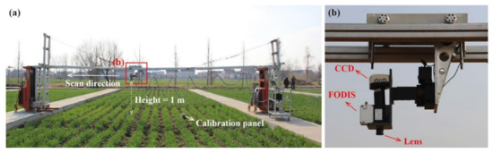
Figure 1.
Near-ground hyperspectral imaging system. (a) Setup of the system in the experimental wheat field, and (b) the onset of the hyperspectral imaging spectrometer (V10E-PS) in the system. FODIS is a fiber optic downwelling irradiance sensor.
2.2.2. Data Preprocessing
The preprocessing of the hyperspectral data consisted of five steps: (1) light intensity correction, (2) dark current correction of the sensor, (3) noise correction, (4) radiometric correction, and (5) selection of sample images. First, the raw images were processed by FODIS (fiber optic downwelling irradiance sensor) correction. FODIS recorded the light intensity of each scan based on the manner of imaging of the spectrometer V10E-PS. The light intensity of raw images was corrected by the software SpecView (SPECIM, Oulu, Finland). Second, dark current correction was used to correct errors in the system. The systematic error is the digital number (DN) value of the hyperspectral image scanned using a covered lens. This error could be directly subtracted in SpecView. Third, the hyperspectral data were smoothed using the minimum noise fraction (MNF) transform in ENVI 5.1 (EXELIS, Boulder, CO, USA). Fourth, the final values of relative reflectance were converted from the DN values, which were converted in turn into radiance:
where Rad, a, and b are the radiance (W·cm−2·sr−1·nm−1), gain, and bias of the sensor, respectively. The values of a and b were automatically acquired by SpecView during hyperspectral imaging. The relative reflectance values were obtained by:
where Radtarget/Reftarget and Radpanel/Refpanel are the radiance/reflectance values of the target images and the calibration panel (Figure 1a), respectively. Fifth, we selected only images in which the wheat was growing evenly and not overexposed. To avoid BRDF (bi-directional reflectance distribution function) effects along the edges, we cropped these images at the central area (i.e., the middle half of the original images).
2.3. Image Classification
We used different methods to classify near-ground hyperspectral images into four classes, i.e., soil, sunlit leaf (SL), shaded leaf (SHL), and panicle. For each class, we selected thousands of the regions of interests (ROIs) during all growth stages of both Exp. 1 and Exp. 2 using ENVI 5.1 (EXELIS, Boulder, CO, USA). The ROIs of Exp. 1 were used as the training set, and the ROIs of Exp. 2 were used as the testing set to calculate the classification accuracy. Accordingly, we could select the best method for image classification (Figure 2a).
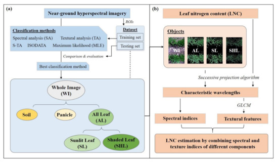
Figure 2.
Flowchart for (a) image classification and (b) leaf nitrogen content (LNC) estimation.
2.3.1. Spectral Analysis (SA)
An advantage of hyperspectral data is the high spectral resolution. Based on the spectral curves of different classes, we could find an optimal spectral combination and corresponding threshold for separating SL, SHL, soil, and panicles [20]. The average reflectance of each class is shown in Figure 3. The four classes had prominent differences in spectral characteristics in the green (540–570 nm), red (670–700 nm), and NIR (760–900 nm) regions. In general, trends of the curves of wheat canopy (SL, SHL, and panicle) were similar. They featured a reflection peak in the green region and a reflection valley in the red region. On the contrary, the soil had no significant reflection peak or valley. In the green region, the reflectance of SL was the highest at 553 nm, while that of SHL and soil were the lowest. In the red region, soil had the highest reflectance and SHL had the lowest reflectance at 680 nm. In the NIR region, the reflectance of SL was much higher than that of the other classes, and these differences were significant. According to these characteristics, the reflectance at 553 nm (R553) was subtracted from that at 680 nm (R680), so that soil with non-positive values could be separated from the wheat canopy with positive values. To increase the differences among different classes, the resulting values were multiplied by the reflectance at 770 nm (R770). Thus, we constructed a spectral classification index (SCI) for image classification:
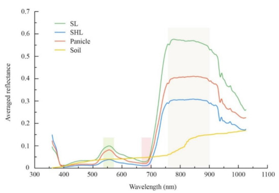
Figure 3.
The average reflectance of sunlit leaf (SL), shaded leaf (SHL), panicle, and soil.
2.3.2. Textural Analysis (TA)
In addition to high spectral resolution, hyperspectral images also have high spatial resolution. We could see the spatial details of the soil, wheat leaves, and panicles in the images acquired. For image classification, we focused on the external structures of these features. Mathematical morphology (MM), a theory and technique for the analysis and processing of geometrical structures, forms the foundation of morphological image processing [46]. It has been widely used in remotely sensed image classification [47,48]. Here, we used MM to extract different image classes. First, edge features were extracted from the processed hyperspectral imagery. Second, morphological filtering was used to remove noise. Third, the basic operators of binary morphology were applied, including dilation, erosion, and opening and closing operators. All processes were performed in MATLAB (V2016a, MathWorks, Natick, MA, USA), and all parameters of morphological operations functions were set as default. The binary images were finally obtained.
2.3.3. Comparison and Evaluation
Based on the intersection of the optimal results from the spectral analysis (SA) and the textural analysis (TA), we combined the two methods as the integrated spectral and textural analysis (S-TA) to separate different classes. In addition, we employed unsupervised (Iterative Self-Organizing Data Analysis Technique Algorithm, ISODATA) and supervised (maximum likelihood, MLE) classification methods as the benchmarks, since both of ISODATA and MLE are classical methods for remotely sensed image classification [49,50,51,52]. The overall accuracy and kappa coefficient were used to evaluate classification accuracy. The overall accuracy (OA) was the ratio of correctly classified samples to the total number of samples [53]:
where N is the total number of samples, r is the number of classification categories, and xii is the number of discriminant samples for samples in the ith category. A confusion matrix is often used to describe virtually the performance of a classification method. All correct predictions are located in the diagonal of the matrix. The kappa coefficient (K) is a more robust measure than simple percent agreement calculation, as it considers the possibility of the agreement occurring by chance. The calculation of K is based on the confusion matrix [53]:
where xi+ and x+i are the sums of the ith row and the ith column of the confusion matrix, respectively, and K ranges from −1 to 1. A larger value of K indicates a better accuracy of image classification. In addition, we used the median run time of different classification methods to evaluate their efficiency by repeating three times for each data set (i.e., Exp. 1 and Exp. 2).
2.4. LNC Estimation
Based on the results of image classification, different classes were extracted from the hyperspectral images. We investigated four target objects for LNC estimation: the whole image (WI), the image of all leaves excluding soil and panicles (AL), the image of sunlit leaf only (SL), and the image of shaded leaf only (SHL) (Figure 2b).
2.4.1. Selection of Characteristic Wavelengths
Owing to the large redundancy in the hyperspectral images, it was necessary to extract the characteristic wavelengths. Note that different feature selection methods would lead to different results of characteristic wavelengths. In this study, we used the successive projections’ algorithm (SPA) to select the characteristic wavelengths for the LNC. The SPA is a forward selection method and a deterministic search technique [54] that uses simple operations in a vector space to minimize variable collinearity. The results of variable selection of the SPA are reproducible, rendering it more robust to the selection of the validation set. It has been widely used for the selection of characteristic wavelengths from hyperspectral data [55]. We applied the SPA in MATLAB (V2016a, MathWorks, Natick, MA, USA) and set the number of characteristics in the range of 5–30. It began with one wavelength and incorporated a new one at each iteration until a specified number N of wavelengths had been reached. The final number of characteristics was determined by root mean-squared error cross-validation (RMSECV). The interested reader can refer to [54] for steps of the SPA, and the given version of the graphical user interface for MATLAB can be downloaded from http://www.ele.ita.br/~kawakami/spa/ (accessed on 5 January 2021).
2.4.2. Calculation of Textural Features
The gray-level co-occurrence matrix (GLCM), the most commonly used texture algorithm, was used to calculate textural features of the four objects (i.e., WI, AL, SL, and SHL). Eight textural features were used: mean (ME), variance (VA), correlation (CC), homogeneity (HO), contrast (CO), dissimilarity (DI), entropy (EN), and second moment (SM). These features reflected the spatial distribution of a textural image (Table 2). To avoid complexity of computation, we calculated the eight textural features of the four objects at the selected characteristic wavelengths for LNC estimation. The features were calculated in ENVI 5.1 (EXELIS, Boulder, CO, USA) with the smallest window size (3 × 3 pixels).
Table 2.
Textural features extracted from gray-level co-occurrence matrix (GLCM) and their representations.
2.4.3. Spectral and Textural Indices
We used three typical forms of two-band combinations for both spectral and textural indices, including the normalized difference index (NDI), ratio index (RI), and difference index (DI):
where x is reflectance at a characteristic wavelength λ for spectral indices, or it is the textural feature (Table 2) at a characteristic wavelength λ for textural indices.
2.4.4. Estimation and Validation
Based on the NDI, RI, and DI, we built linear models of the LNC for the four objects (i.e., WI, AL, SL, and SHL) during all stages of wheat growth. Each of the estimated models were calibrated based on data from Exp. 1 and were validated using data from Exp. 2. The accuracy of the LNC models was evaluated by the coefficient of determination (R2) and the relative root mean-squared error (RRMSE):
where x, y, and n are the estimated LNC value, LNC measurements, and the number of samples, respectively.
3. Results
3.1. Near-Ground Hyperspectral Image Classification
Figure 4 shows the SCI frequency of the four classes (i.e., soil, panicle, SL, and SHL) in different stages. The ranges of the SCI values of soil, SL, and SHL were clearly demarcated in all stages. According to their ranges for the target components (Table 3), the soil, SHL, and SL could be separated as soil < 0.29 < SHL < 2.1 < SL. However, panicles could not be distinguished from the other components by SCI (Figure 4d and Table 3). By contrast, textural analysis based on the MM was able to extract panicles in the heading stage (Figure 5).
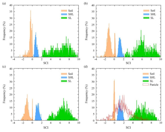
Figure 4.
Histogram-based statistical analysis of target components at the (a) greening, (b) jointing, (c) booting, and (d) heading stages based on the spectral classification index (SCI).
Table 3.
The maximum and minimum SCI values of the target components at different stages. The values in the last column (all stages) are the corresponding minimum or maximum values in a row.
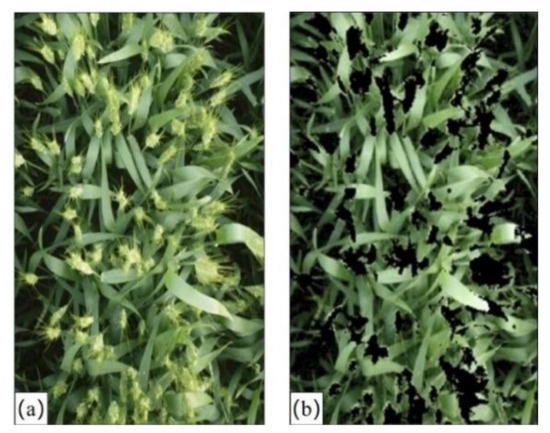
Figure 5.
A comparison between (a) the original image at heading stage and (b) the masked results of the panicles based on textural analysis (TA).
To further analyze the accuracy of different classification methods for each target class, a confusion matrix in the heading stage was shown in Table 4, since only the imagery in the heading stage contained all the four targets (especially panicles). For the target class SL, all methods classified part of it incorrectly as a panicle. The highest percentage of SL being incorrectly classified as panicles was 8.94% using the SA, and the lowest was 0.66% using the S-TA. In addition to being misclassified as panicles, 17.54% of SL was misclassified as SHL by the TA. For the target class SHL, ISODATA delivered the poorest performance, with the highest misclassification of 72.43%, including 37.97% as soil, 34.07% as panicle, and 0.40% as SL. On the contrary, the S-TA delivered the best performance because it recorded the lowest rate of misclassification of the SHL (1.08%). For the panicle as target class, most methods misclassified it as a wheat leaf (SL and SHL), but the S-TA correctly extracted all panicles. For soil as the target class, most methods were able to identify all soil pixels from the hyperspectral images, but the ISODATA and MLE misclassified 0.21% and 0.02% of the soils as panicles, respectively.
Table 4.
The confusion matrix (%) of each class based on different classification methods in the heading stage.
In general, the classification accuracy of the S-TA in all stages was the highest (OA = 97.8%, K = 0.971), which is followed by the MLE (OA = 94.5%, K = 0.942) (Table 5). However, the median run time of the MLE was more than six times longer than that of the S-TA. The unsupervised method ISODATA was the least efficient, with a value of OA of 71.6%, K = 0.632, and run time of 85 min.
Table 5.
The classification accuracy and efficiency of different methods for all stages.
3.2. Changes in Reflectance of Different Objects under Different Conditions
Based on the results of image classification, we compared the averaged changes in the reflectance of the four objects (i.e., WI, AL, SL, and SHL) under different conditions (Figure 6). In general, the reflectance of WI increased, and gaps among the reflectance of AL, SL, and SHL decreased when the nitrogen rate increased from N0 to N1 (Figure 6a–c) and planting density increased from D1 to D2 (Figure 6b,e). This is because the canopy coverage increased and the canopy spectra were less affected by the background of soil. Moreover, the spectra of different varieties of wheat were different (Figure 6b,d), which might have been related to the type of wheat plant. Yangmai 8 (V1) is erect and thus was more affected by the background of soil than the spread type (V2: Shengxuan 6). Regardless of the different conditions, the spectra of AL with the background of soil removed had a blue shift in the red edge region. This indicates that the soil as background would cause a red edge shift of the spectra of the wheat canopy.
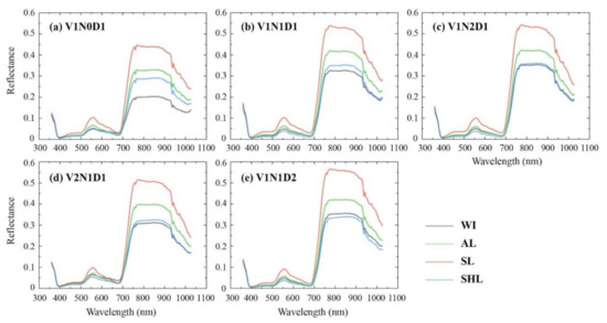
Figure 6.
Changes in the reflectance of different objects under different conditions: (a) V1N0D1, (b) V1N1D1, (c) V1N2D1, (d) V2N1D1, and (e) V1N1D2. The descriptions of different conditions are provided in Table 1.
3.3. LNC Estimation Using Spectral and Texture Indices of Different Objects
The characteristic wavelengths of different objects were extracted by the SPA and sorted by sensitivity to the LNC (Table 6). Based on Equations (6)–(8), we constructed spectral and textural indices of the four objects (i.e., WI, AL, SL, and SHL). By comparing all combinations of the characteristic wavelengths or textural features at these wavelengths, we selected the optimal indices (spectral index (SI), textural index (TI), and spectral and textural indices (STI)) for each object (Table 7). In terms of their optimal composition, most indices were composed of one NIR wavelength and one visible wavelength. The most commonly selected textural feature was the second moment (SM), which was followed by the mean (ME). The optimal STIs of the four objects were the types of combination of the NDSTI with different spectral and textural features. For different objects, the accuracies of LNC calibration of SL and SHL were poor, with lower than 0.54. On the contrary, the LNC calibrations of AL were the best, with higher than 0.70. In terms of spectral and textural indices, the LNC~STI models were generally more accurate than the LNC~SI and LNC~TI models of each object. Although the accuracy of the LNC~SI models was not much lower than that of the LNC~STI models, the LNC~SI models were not robust. Conversely, LNC estimations based on the STI were more stable. For example, the accuracy of validation of the LNC~DSI model of AL decreased to values of of 0.66 and RRMSE of 13.9% (compared with an of 0.75 and RRMSEc of 16.2%), while the of the LNC~NDSTI model was 0.83, and its RRMSEv was 10.9%. Moreover, although the accuracy of the LNC~NDSI model during calibration was the highest for SHL with an of 0.52 and RRMSEc of 15.4%, that in validation decreased to an of 0.27 and RRMSEv of 23.1%. Overall, the best LNC estimations during both calibration and validation were obtained by the LNC~NDSTI (R931.88, T432.38SM) model of AL.
Table 6.
The characteristic wavelengths of different objects using the successive projections algorithm (SPA).
Table 7.
The optimal spectral index (SI), textural index (TI), and spectral and textural index (STI) of the four objects, and the corresponding statistics for LNC estimations and validations.
Based on the overall optimal indices of the NDSTI (R931.88, T432.38SM) of AL, Figure 7 shows the validation of LNC estimations under different conditions and in different stages. In general, the scatters were distributed along the 1:1 line. The LNC was accurately estimated, regardless of different rates of nitrogen (Figure 7a), planting densities (Figure 7b), wheat varieties (Figure 7c), and stages of growth (Figure 7d).
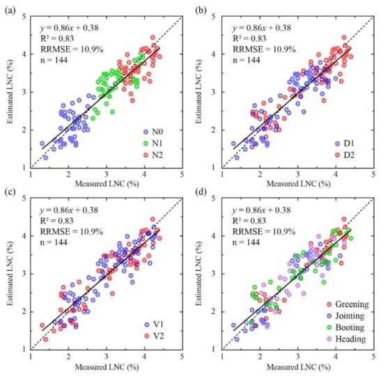
Figure 7.
The validations of LNC estimations based on the optimal indices of NDSTI (R931.88, T432.38SM) of the all leaves (AL) object under (a) different nitrogen rates, (b) different planting densities, (c) different wheat varieties, and (d) in different growth stages. The descriptions of different conditions are given in Table 1.
4. Discussion
4.1. Assessment of Classification Methods
We compared the performance of five classification methods: ISODATA, MLE, SA, TA, and S-TA. ISODATA is an unsupervised method of classification that could not distinguish different target components, and its overall classification accuracy and kappa coefficient were the lowest (Table 5). Compared with ISODATA, the overall accuracy and kappa coefficient of supervised classification (MLE) were 22.9% and 0.31 higher, respectively (Table 5). This shows that selecting appropriate and accurate training samples is crucial to the accuracy of classification. However, different kinds of image data require different training samples, and the use of supervised classification requires sophisticated hardware for data processing. In this study, the median run time of the MLE was the longest (100 min): 1.2 times that of ISODATA. The fastest classification method was the SA. It was constructed as a decision tree of the SCI based on the spectral characteristics of SL, SHL, panicles, and soil (Figure 2). Our results show that the differences in SCI among soil, SL, and SHL were clear (Figure 4), but panicles were easily misclassified as the other components by the SA (Table 4). This suggests that the SCI could not be used to extract wheat panicles, even though it was the optimal index according to our results. We might find a spectral index to distinguish leaves from panicles, but the limitations of the SA can affect the results of classification. A decision tree classification has a boundary effect, such that some pixels with values close to the threshold are misclassified [20].
Given that the spectral classifications (i.e., ISODATA, MLE, SA) are strongly dependent on differences in the spectral values of pixels [21], we investigated the TA based on the structure of spatial information of the images. Compared with the SA, the TA could extract panicles more accurately in the heading stage (Figure 5 and Table 4) because the spectral characteristics of wheat panicles are similar to those of leaves (Figure 2), but their textural characteristics are different. This suggests that the TA can improve classification accuracy by mitigating spectral confusion among spectrally similar classes [33]. However, the classification accuracy of the TA did not improve for all growth stages compared with that of the SA, and its overall accuracy and kappa coefficient were similar to those of the SA (Table 5). When we used only the TA, SL and SHL could not be distinguished (Table 4), owing to similar textural features of the leaves, but SA could help in this case. By combining the SA and TA, the S-TA boasts the complementary advantages of spectral and textural information. Moreover, compared with traditional classification methods, the S-TA was able to classify different components of winter wheat with higher accuracy, better robustness, and in shorter time (Table 5).
4.2. Soil Background and Shadow Effects in LNC Estimation
Soil as background affects the spectra of the crop canopy owing to the combined effects of planting density, canopy structure, and growth stage [56], which in turn affect LNC estimation [10]. The experimental design satisfactorily represented an environment in which the crop and soil coexisted in different conditions of planting density, wheat variety, and nitrogen rate during the greening, jointing, booting, and heading stages. Our results showed that the soil background would affect the spectral response of winter wheat regardless of different conditions (Figure 6). Furthermore, the correlations between LNC and the canopy indices were significantly affected by the soil background (Table 7), which is consistent with previous studies [10]. When excluding the soil background from WI, R2 increased and RRMSE decreased for AL in both LNC calibration and validation (Table 7). Therefore, the soil background should be reduced to improve the LNC estimation of wheat.
In spite of the soil background, shadow effects can influence the accuracy of LNC estimation. However, previous studies have often focused on the sunlit pixels of the canopy for monitoring crops while neglecting shadow effects [57,58,59]. Our results showed low correlations between the indices and the LNC in SL without using SHL pixels (Table 7), which is mainly because the multiple scatterings among SHL would lead to a longer optical length and weaker signal strength [60,61] that would enhance the apparent absorptive characteristics of the leaves [62,63,64]. Zhou et al. [20] also calculated the gain from the SHL pixels, but for the estimation of chlorophyll content in rice, and they obtained higher accuracy when using SHL than when using SL. However, our results showed that the accuracies of LNC estimations in SHL and SL were similar, and the highest was in AL (Table 7). This might have occurred because LNC represents information on the wheat population at the leaf level, but SL pixels represent only parts of wheat leaves. Therefore, we suggest using the features of all leaves (including SL and SHL) to estimate the LNC of wheat.
4.3. Further Improvement of the LNC Estimation
Assessing the predictive performance of different indices showed that STIs provided higher accuracy of estimation of the LNC of wheat. In addition, the LNC estimation was the most stable when applied to the AL object regardless of different conditions (nitrogen rate, planting density, and wheat variety) in different growth stages (Figure 7). The premise is to eliminate the confounding effects of other components on the reflectance spectra of the canopy [18]. The TA could exclude soil background and panicles, thereby improving the LNC estimation. In contrast, the contribution of textural index to the LNC estimation was not significant (Table 7). The mechanistic link between LNC and textural index should be further investigated. The S-TA can provide a good compromise between accuracy and efficiency in extracting the features of all wheat leaves from the canopy image. Therefore, the integration of spectral and textural information offers a promising approach to monitor the nitrogen content of plants to enable precision farming throughout the growing season of winter wheat.
In particular, near-ground hyperspectral imagery with ultra-high spatial and spectral resolutions can provide more details. Thus, we should investigate the effects of STI selection, spatial resolution, and the estimated models on crop monitoring. When selecting optimal texture features, a moving window and image bands of appropriate sizes should be considered [65]. As the window size does not have a significant impact on experimental crop fields, where crops are often planted in rows [33], we used the recommended window size (3 × 3). However, the effect of window size should be investigated in future work, especially for large and heterogeneous fields. Moreover, textural features are computed from the spectral images, and so the corresponding spectral distribution is represented in image space [66]. Since the results of characteristic wavelengths might be different (or sometimes contradictory) from different feature selection methods, the characteristic wavelengths for LNC from the SPA in this study should be further investigated. We should compare the SPA to other methods (e.g., principal component analysis, particle swarm algorithm, maximum noise fraction, etc.) and investigate their impact on LAI estimations in the future work. Previous studies have focused on applications of spectral and textural analyses using satellite data (mostly Landsat TM) [27,67] and images captured by unmanned aerial vehicles (UAVs) (mostly digital and multispectral cameras) [28,33]. As the spatial resolution increases, more spatial details can be observed, but ultra-high spatial imagery often causes noise [68,69]. Therefore, different methods of sensitivity analysis and texture algorithms should be investigated. The impact of spatial resolution on image classification and crop monitoring should also be further assessed, and the efficiency of application can be improved at the optimal spatial resolution [18]. In addition to STI selection and spatial resolution, integrating spectral and textural information can help extend the potential of use of the estimation models. Although the simple statistical regression models of the LNC and STI showed good robustness, the potential for the use of large amounts of data needs to be further explored. In particular, machine learning might benefit LNC estimation as textural features provide a new dimension and enlarge the training data. In this regard, more prediction algorithms will be investigated in our future work.
5. Conclusions
We used near-ground hyperspectral data to estimate the LNC of winter wheat through the entire growing season in two-year field experiments under different nitrogen rates, planting densities, and wheat varieties. To classify the soil, panicles, sunlit leaves (SL), and shadowed leaves (SHL), the combination of spectral and textural analysis (S-TA) provided a good compromise between accuracy and efficiency (overall accuracy = 97.8%, kappa coefficient = 0.971, and run time = 14 min) compared with unsupervised classification (ISODATA), supervised classification (MLE), spectral analysis (SA), and textural analysis (TA). Based on the S-TA, we classified four objects—the whole image (WI), all leaves (AL), SL, and SHL—and extracted three indices (SI, TI, and STI) from them. All AL-derived indices achieved more stable relationships with the LNC than the WI-, SL-, and SHL-derived indices due to the elimination of the soil background and the consideration of shadow effects. Therefore, we suggest using the features of all leaves (including SL and SHL) to estimate LNC. In particular, the AL-derived NDSTI (R931.88, T432.38SM) delivered the best performance in terms of LNC estimations in both calibration ( = 0.78, RRMSEc = 13.5%) and validation ( = 0.83, RRMSEv = 10.9%). It suggests that the integration of spectral and textural information offers a promising approach to both image classification and crop monitoring. In the future work, the effects of STI selection, spatial resolution, and the estimated models need to be further investigated.
Author Contributions
Conceptualization, X.Y.; methodology, J.J. and X.Y.; validation, J.J. and J.Z.; formal analysis, J.J.; writing—original draft preparation, J.J. and X.Y.; writing—review and editing, all authors. All authors have read and agreed to the published version of the manuscript.
Funding
This research was funded by the National Natural Science Foundation of China, grant number 31671582, 31971780; Key Projects (Advanced Technology) of Jiangsu Province, grant number BE 2019383; the Jiangsu Collaborative Innovation Center for Modern Crop Production (JCICMCP); Qinghai Project of Transformation of Scientific and Technological Achievements, grant number 2018-NK-126; and Xinjiang Corps Great Science and Technology Projects, grant number 2018AA00403.
Institutional Review Board Statement
Not applicable.
Informed Consent Statement
Not applicable.
Data Availability Statement
Not applicable.
Conflicts of Interest
The authors declare no conflict of interest.
References
- Benedetti, R.; Rossini, P. On the use of NDVI profiles as a tool for agricultural statistics: The case study of wheat yield estimate and forecast in Emilia Romagna. Remote Sens. Environ. 1993, 45, 311–326. [Google Scholar] [CrossRef]
- Jiang, J.; Cai, W.; Zheng, H.; Cheng, T.; Tian, Y.; Zhu, Y.; Ehsani, R.; Hu, Y.; Niu, Q.; Gui, L. Using Digital Cameras on an Unmanned Aerial Vehicle to Derive Optimum Color Vegetation Indices for Leaf Nitrogen Concentration Monitoring in Winter Wheat. Remote Sens. 2019, 11, 2667. [Google Scholar] [CrossRef]
- Fitzgerald, G.; Rodriguez, D.; Leary, O.G. Measuring and predicting canopy nitrogen nutrition in wheat using a spectral index—The canopy chlorophyll content index (CCCI). Field Crop. Res. 2010, 116, 318–324. [Google Scholar] [CrossRef]
- Hansen, P.; Schjoerring, J. Reflectance measurement of canopy biomass and nitrogen status in wheat crops using normalized difference vegetation indices and partial least squares regression. Remote Sens. Environ. 2003, 86, 542–553. [Google Scholar] [CrossRef]
- Li, D.; Wang, X.; Zheng, H.; Zhou, K.; Yao, X.; Tian, Y.; Zhu, Y.; Cao, W.; Cheng, T. Estimation of area-and mass-based leaf nitrogen contents of wheat and rice crops from water-removed spectra using continuous wavelet analysis. Plant Methods 2018, 14, 76. [Google Scholar] [CrossRef]
- Zheng, H.; Cheng, T.; Li, D.; Zhou, X.; Yao, X.; Tian, Y.; Cao, W.; Zhu, Y. Evaluation of RGB, color-infrared and multispectral images acquired from unmanned aerial systems for the estimation of nitrogen accumulation in rice. Remote Sens. 2018, 10, 824. [Google Scholar] [CrossRef]
- Yao, Y.; Miao, Y.; Cao, Q.; Wang, H.; Gnyp, M.L.; Bareth, G.; Khosla, R.; Yang, W.; Liu, F.; Liu, C. In-season estimation of rice nitrogen status with an active crop canopy sensor. IEEE J. Sel. Top. Appl. Earth Obs. Remote Sens. 2014, 7, 4403–4413. [Google Scholar] [CrossRef]
- Yao, X.; Zhu, Y.; Tian, Y.; Feng, W.; Cao, W. Exploring hyperspectral bands and estimation indices for leaf nitrogen accumulation in wheat. Int. J. Appl. Earth Obs. Geoinf. 2010, 12, 89–100. [Google Scholar] [CrossRef]
- Feng, W.; Yao, X.; Zhu, Y.; Tian, Y.; Cao, W. Monitoring leaf nitrogen status with hyperspectral reflectance in wheat. Eur. J. Agron. 2008, 28, 394–404. [Google Scholar] [CrossRef]
- Yao, X.; Ren, H.; Cao, Z.; Tian, Y.; Cao, W.; Zhu, Y.; Cheng, T. Detecting leaf nitrogen content in wheat with canopy hyperspectrum under different soil backgrounds. Int. J. Appl. Earth Obs. Geoinf. 2014, 32, 114–124. [Google Scholar] [CrossRef]
- Li, F.; Mistele, B.; Hu, Y.; Chen, X.; Schmidhalter, U. Reflectance estimation of canopy nitrogen content in winter wheat using optimised hyperspectral spectral indices and partial least squares regression. Eur. J. Agron. 2014, 52, 198–209. [Google Scholar] [CrossRef]
- Liu, H.; Zhu, H.; Wang, P. Quantitative modelling for leaf nitrogen content of winter wheat using UAV-based hyperspectral data. Int. J. Remote Sens. 2017, 38, 2117–2134. [Google Scholar] [CrossRef]
- Haboudane, D.; Miller, J.R.; Tremblay, N.; Tejada, Z.P.J.; Dextraze, L. Integrated narrow-band vegetation indices for prediction of crop chlorophyll content for application to precision agriculture. Remote Sens. Environ. 2002, 81, 416–426. [Google Scholar] [CrossRef]
- Vigneau, N.; Ecarnot, M.; Rabatel, G.; Roumet, P. Potential of field hyperspectral imaging as a non destructive method to assess leaf nitrogen content in Wheat. Field Crop. Res. 2011, 122, 25–31. [Google Scholar] [CrossRef]
- Onoyama, H.; Ryu, C.; Suguri, M.; Iida, M. Nitrogen prediction model of rice plant at panicle initiation stage using ground-based hyperspectral imaging: Growing degree-days integrated model. Precis. Agric. 2015, 16, 558–570. [Google Scholar] [CrossRef]
- Jay, S.; Hadoux, X.; Gorretta, N.; Rabatel, G. Potential of Hyperspectral Imagery for Nitrogen Content Retrieval in Sugar Beet Leaves; AgEng: Évora, Portugal, 2014. [Google Scholar]
- Miphokasap, P.; Honda, K.; Vaiphasa, C.; Souris, M.; Nagai, M. Estimating canopy nitrogen concentration in sugarcane using field imaging spectroscopy. Remote Sens. 2012, 4, 1651–1670. [Google Scholar] [CrossRef]
- Zhou, K.; Cheng, T.; Zhu, Y.; Cao, W.; Ustin, S.L.; Zheng, H.; Yao, X.; Tian, Y. Assessing the Impact of Spatial Resolution on the Estimation of Leaf Nitrogen Concentration Over the Full Season of Paddy Rice Using Near-Surface Imaging Spectroscopy Data. Front. Plant Sci. 2018, 9, 964. [Google Scholar] [CrossRef] [PubMed]
- Adeline, K.; Chen, M.; Briottet, X.; Pang, S.; Paparoditis, N. Shadow detection in very high spatial resolution aerial images: A comparative study. ISPRS J. Photogramm. Remote Sens. 2013, 80, 21–38. [Google Scholar] [CrossRef]
- Zhou, K.; Deng, X.; Yao, X.; Tian, Y.; Cao, W.; Zhu, Y.; Ustin, S.L.; Cheng, T. Assessing the Spectral Properties of Sunlit and Shaded Components in Rice Canopies with Near-Ground Imaging Spectroscopy Data. Sensors 2017, 17, 578. [Google Scholar] [CrossRef]
- Banerjee, K.; Krishnan, P. Normalized Sunlit Shaded Index (NSSI) for characterizing the moisture stress in wheat crop using classified thermal and visible images. Ecol. Indic. 2020, 110. [Google Scholar] [CrossRef]
- Dongyan, Z. Diagnosis Mechanism and Methods of Crop Chlorophyll Information Based on Hypersepctral Imaging Technology; Zhejiang University: Hangzhou, China, 2012. (in Chinese) [Google Scholar]
- Gnyp, M.L.; Miao, Y.; Yuan, F.; Ustin, S.L.; Yu, K.; Yao, Y.; Huang, S.; Bareth, G. Hyperspectral canopy sensing of paddy rice aboveground biomass at different growth stages. Field Crop. Res. 2014, 155, 42–55. [Google Scholar] [CrossRef]
- Bharati, M.H.; Liu, J.J.; MacGregor, J.F. Image texture analysis: Methods and comparisons. Chemom. Intell. Lab. Syst. 2004, 72, 57–71. [Google Scholar] [CrossRef]
- Haralick, R.M.; Shanmugam, K.; Dinstein, I.H. Textural features for image classification. IEEE Trans. Syst. Man Cybern. 1973, 6, 610–621. [Google Scholar] [CrossRef]
- Haralick, R.M. Statistical and structural approaches to texture. Proc. IEEE 1979, 67, 786–804. [Google Scholar] [CrossRef]
- Lu, D.; Batistella, M. Exploring TM image texture and its relationships with biomass estimation in Rondônia, Brazilian Amazon. Acta Amaz. 2005, 35, 249–257. [Google Scholar] [CrossRef]
- Zheng, H.; Ma, J.; Zhou, M.; Li, D.; Yao, X.; Cao, W.; Zhu, Y.; Cheng, T. Enhancing the Nitrogen Signals of Rice Canopies across Critical Growth Stages through the Integration of Textural and Spectral Information from Unmanned Aerial Vehicle (UAV) Multispectral Imagery. Remote Sens. 2020, 12, 957. [Google Scholar] [CrossRef]
- Ashoori, H.; Fahimnejad, H.; Alimohammadi, A.; Soofbaf, S. Evaluation of the usefulness of texture measures for crop type classification by Hyperion data. Int. Arch. Spat. Inf. Sci. 2008, 37, 999–1006. [Google Scholar]
- Rellier, G.; Descombes, X.; Falzon, F.; Zerubia, J. Texture feature analysis using a Gauss-Markov model in hyperspectral image classification. IEEE Trans. Geosci. Remote Sens. 2004, 42, 1543–1551. [Google Scholar] [CrossRef]
- Qian, Y.; Ye, M.; Zhou, J. Hyperspectral image classification based on structured sparse logistic regression and three-dimensional wavelet texture features. IEEE Trans. Geosci. Remote Sens. 2012, 51, 2276–2291. [Google Scholar] [CrossRef]
- Zhang, X.; Sun, Y.; Shang, K.; Zhang, L.; Wang, S. Crop classification based on feature band set construction and object-oriented approach using hyperspectral images. IEEE J. Sel. Top. Appl. Earth Obs. Remote Sens. 2016, 9, 4117–4128. [Google Scholar] [CrossRef]
- Zheng, H.; Cheng, T.; Zhou, M.; Li, D.; Yao, X.; Tian, Y.; Cao, W.; Zhu, Y. Improved estimation of rice aboveground biomass combining textural and spectral analysis of UAV imagery. Precis. Agric. 2018, 20, 611–629. [Google Scholar] [CrossRef]
- Yue, J.; Yang, G.; Tian, Q.; Feng, H.; Xu, K.; Zhou, C. Estimate of winter-wheat above-ground biomass based on UAV ultrahigh-ground-resolution image textures and vegetation indices. ISPRS J. Photogramm. Remote Sens. 2019, 150, 226–244. [Google Scholar] [CrossRef]
- Li, S.; Yuan, F.; Karim, A.U.S.T.; Zheng, H.; Cheng, T.; Liu, X.; Tian, Y.; Zhu, Y.; Cao, W.; Cao, Q. Combining Color Indices and Textures of UAV-Based Digital Imagery for Rice LAI Estimation. Remote Sens. 2019, 11, 1763. [Google Scholar] [CrossRef]
- Dube, T.; Mutanga, O. Investigating the robustness of the new Landsat-8 Operational Land Imager derived texture metrics in estimating plantation forest aboveground biomass in resource constrained areas. ISPRS J. Photogramm. Remote Sens. 2015, 108, 12–32. [Google Scholar] [CrossRef]
- Yang, W.H.; Peng, S.; Huang, J.; Sanico, A.L.; Buresh, R.J.; Witt, C. Using leaf color charts to estimate leaf nitrogen status of rice. Agron. J. 2003, 95, 212–217. [Google Scholar]
- Singh, B.; Singh, Y.; Ladha, J.K.; Bronson, K.F.; Balasubramanian, V.; Singh, J.; Khind, C.S. Chlorophyll meter–and leaf color chart–based nitrogen management for rice and wheat in Northwestern India. Agron. J. 2002, 94, 821–829. [Google Scholar] [CrossRef]
- Da Silva Oliveira, M.W. Texture Analysis on Leaf Images for Early Nutritional Diagnosis in Maize Culture; University of São Paulo: São Paulo, Brazil, 2016. [Google Scholar]
- Romualdo, L.; Luz, P.; Devechio, F.; Marin, M.; Zúñiga, A.; Bruno, O.; Herling, V. Use of artificial vision techniques for diagnostic of nitrogen nutritional status in maize plants. Comput. Electron. Agric. 2014, 104, 63–70. [Google Scholar] [CrossRef]
- Kimes, D.; Newcomb, W.; Tucker, C.; Zonneveld, I.; Van Wijngaarden, W.; De Leeuw, J.; Epema, G. Directional reflectance factor distributions for cover types of Northern Africa. Remote Sens. Environ. 1985, 18, 1–19. [Google Scholar] [CrossRef]
- Leblanc, S.G.; Chen, J.M.; Cihlar, J. NDVI directionality in boreal forests: A model interpretation of measurements. Canadian J. Remote Sens. 1997, 23, 369–380. [Google Scholar] [CrossRef]
- Sun, H.; Li, M.Z.; Zhao, Y.; Zhang, Y.E.; Wang, X.M.; Li, X.H. The spectral characteristics and chlorophyll content at winter wheat growth stages. Spectrosc. Spectr. Anal. 2010, 30, 192–196. [Google Scholar]
- Yue, J.; Feng, H.; Yang, G.; Li, Z. A comparison of regression techniques for estimation of above-ground winter wheat biomass using near-surface spectroscopy. Remote Sens. 2018, 10, 66. [Google Scholar] [CrossRef]
- Bremner, J.M.; Mulvaney, C. Nitrogen—total. Methods Soil Anal. Part. 2 Chem. Microbiol. Prop. 1983, 9, 595–624. [Google Scholar]
- Haralick, R.M.; Sternberg, S.R.; Zhuang, X. Image analysis using mathematical morphology. IEEE Trans. Pattern Anal. Mach. Intell. 1987, 4, 532–550. [Google Scholar] [CrossRef] [PubMed]
- Chen, T.; Trinder, J.C.; Niu, R. Object-oriented landslide mapping using ZY-3 satellite imagery, random forest and mathematical morphology, for the Three-Gorges Reservoir, China. Remote Sens. 2017, 9, 333. [Google Scholar] [CrossRef]
- Ghamisi, P.; Maggiori, E.; Li, S.; Souza, R.; Tarablaka, Y.; Moser, G.; De Giorgi, A.; Fang, L.; Chen, Y.; Chi, M. New frontiers in spectral-spatial hyperspectral image classification: The latest advances based on mathematical morphology, Markov random fields, segmentation, sparse representation, and deep learning. IEEE Geosci. Remote Sens. Mag. 2018, 6, 10–43. [Google Scholar] [CrossRef]
- Abbas, A.W.; Minallh, N.; Ahmad, N.; Abid, S.A.R.; Khan, M.A.A. K-Means and ISODATA Clustering Algorithms for Landcover Classification Using Remote Sensing. 2016, Volume 48. ISSN 1813-1743. Available online: https://sujo-old.usindh.edu.pk/index.php/SURJ/article/view/2358 (accessed on 5 January 2021).
- Hemalatha, S.; Anouncia, S.M. Unsupervised segmentation of remote sensing images using FD based texture analysis model and ISODATA. Int. J. Ambient Comput. Intell. (IJACI) 2017, 8, 58–75. [Google Scholar] [CrossRef]
- Peng, J.; Li, L.; Tang, Y.Y. Maximum likelihood estimation-based joint sparse representation for the classification of hyperspectral remote sensing images. IEEE Trans. Neural Netw. Learn. Syst. 2018, 30, 1790–1802. [Google Scholar] [CrossRef]
- Strahler, A.H. The use of prior probabilities in maximum likelihood classification of remotely sensed data. Remote Sens. Environ. 1980, 10, 135–163. [Google Scholar] [CrossRef]
- Congalton, R.G.; Green, K. Assessing the Accuracy of Remotely Sensed Data: Principles and Practices; CRC Press: Boca Raton, FL, USA, 2019. [Google Scholar]
- Araújo, M.C.U.; Saldanha, T.C.B.; Galvao, R.K.H.; Yoneyama, T.; Chame, H.C.; Visani, V. The successive projections algorithm for variable selection in spectroscopic multicomponent analysis. Chemom. Intell. Lab. Syst. 2001, 57, 65–73. [Google Scholar] [CrossRef]
- Wang, Y.J.; Li, L.Q.; Shen, S.S.; Liu, Y.; Ning, J.M.; Zhang, Z.Z. Rapid detection of quality index of postharvest fresh tea leaves using hyperspectral imaging. J. Sci. Food Agric. 2020, 100, 3803–3811. [Google Scholar] [CrossRef] [PubMed]
- Rondeaux, G.; Steven, M.; Baret, F. Optimization of soil-adjusted vegetation indices. Remote Sens. Environ. 1996, 55, 95–107. [Google Scholar] [CrossRef]
- Malenovský, Z.; Homolová, L.; Milla, Z.R.; Lukeš, P.; Kaplan, V.; Hanuš, J.; Etchegorry, G.J.P.; Schaepman, M.E. Retrieval of spruce leaf chlorophyll content from airborne image data using continuum removal and radiative transfer. Remote Sens. Environ. 2013, 131, 85–102. [Google Scholar] [CrossRef]
- Zhang, Y.; Chen, J.M.; Miller, J.R.; Noland, T.L. Leaf chlorophyll content retrieval from airborne hyperspectral remote sensing imagery. Remote Sens. Environ. 2008, 112, 3234–3247. [Google Scholar] [CrossRef]
- Tejada, Z.P.J.; Miller, J.R.; Harron, J.; Hu, B.; Noland, T.L.; Goel, N.; Mohammed, G.H.; Sampson, P. Needle chlorophyll content estimation through model inversion using hyperspectral data from boreal conifer forest canopies. Remote Sens. Environ. 2004, 89, 189–199. [Google Scholar] [CrossRef]
- Chen, J.M.; Leblanc, S.G. Multiple-scattering scheme useful for geometric optical modeling. IEEE Trans. Geosci. Remote Sens. 2001, 39, 1061–1071. [Google Scholar] [CrossRef]
- Zhou, K.; Guo, Y.; Geng, Y.; Zhu, Y.; Cao, W.; Tian, Y. Development of a novel bidirectional canopy reflectance model for row-planted rice and wheat. Remote Sens. 2014, 6, 7632–7659. [Google Scholar] [CrossRef]
- Kokaly, R.F.; Despain, D.G.; Clark, R.N.; Livo, K.E. Mapping vegetation in Yellowstone National Park using spectral feature analysis of AVIRIS data. Remote Sens. Environ. 2003, 84, 437–456. [Google Scholar] [CrossRef]
- Salisbury, J.W.; Milton, N.; Walsh, P. Significance of non-isotropic scattering from vegetation for geobotanical remote sensing. Int. J. Remote Sens. 1987, 8, 997–1009. [Google Scholar] [CrossRef]
- Baret, F.; Jacquemoud, S.; Guyot, G.; Leprieur, C. Modeled analysis of the biophysical nature of spectral shifts and comparison with information content of broad bands. Remote Sens. Environ. 1992, 41, 133–142. [Google Scholar] [CrossRef]
- Chen, D.; Stow, D.; Gong, P. Examining the effect of spatial resolution and texture window size on classification accuracy: An urban environment case. Int. J. Remote Sens. 2004, 25, 2177–2192. [Google Scholar] [CrossRef]
- Ning, S. Remote sensing image texture analysis and fractal assessment. J. Wuhan Tech. Univ. Surv. Mapp. 1998, 23, 370–373. [Google Scholar]
- Lu, D. Aboveground biomass estimation using Landsat TM data in the Brazilian Amazon. Int. J. Remote Sens. 2005, 26, 2509–2525. [Google Scholar] [CrossRef]
- Hall, O.; Dahlin, S.; Marstorp, H.; Archila Bustos, M.F.; Öborn, I.; Jirström, M. Classification of maize in complex smallholder farming systems using UAV imagery. Drones 2018, 2, 22. [Google Scholar] [CrossRef]
- Li, M.; Zang, S.; Zhang, B.; Li, S.; Wu, C. A review of remote sensing image classification techniques: The role of spatio-contextual information. Eur. J. Remote Sens. 2014, 47, 389–411. [Google Scholar] [CrossRef]


Publisher’s Note: MDPI stays neutral with regard to jurisdictional claims in published maps and institutional affiliations. |
© 2021 by the authors. Licensee MDPI, Basel, Switzerland. This article is an open access article distributed under the terms and conditions of the Creative Commons Attribution (CC BY) license (http://creativecommons.org/licenses/by/4.0/).