Quantifying Optically Derived Two-Dimensional Wave-Averaged Currents in the Surf Zone

Abstract

Complex two-dimensional nearshore current patterns are generated by feedbacks between sub-aqueous morphology and momentum imparted on the water column by breaking waves, winds, and tides. These non-stationary features, such as rip currents and circulation cells, respond to changing environmental conditions and underlying morphology. However, using fixed instruments to observe nearshore currents is limiting due to the high costs and logistics necessary to achieve adequate spatial sampling resolution. A new technique for processing surf-zone imagery, WAMFlow, quantifies fluid velocities to reveal complex, multi-scale (10 s–1000 s meters) nearshore surface circulation patterns. We apply the concept of a wave-averaged movie (WAM) to measure surf-zone circulation patterns on spatial scales of kilometers in the alongshore and 100 s of meters in the cross-shore. The approach uses a rolling average of 2 Hz optical imagery, removing the dominant optical clutter of incident waves, to leave the residual foam or water turbidity features carried by the flow. These residual features are tracked as quasi-passive tracers in space and time using optical flow, which solves for u and v as a function of image intensity gradients in x, y, and t. Surf zone drifters were deployed over multiple days with varying nearshore circulations to validate the optically derived flow patterns. Root mean square error are reduced to 0.1 m per second after filtering based on image attributes. The optically derived patterns captured longshore currents, rip currents, and gyres within the surf zone. Quantifying nearshore circulation patterns using low-cost image platforms and open-source computer vision algorithms presents the potential to further our understanding of fundamental surf zone dynamics.

1. Introduction

Wave-averaged currents are a fundamental driver of numerous nearshore processes, including rip currents that claim lives [1], alongshore currents impacting ecosystem health and pollutant transport [2], and flow gradients altering nearshore morphology [3]. Flows can be forced by breaking wave momentum [4], pressure gradients, and low-frequency motions [5]. Competition between forcing and dissipation yield varying velocities (decimeters per second) over large spatial scales (10²–10⁴ m). Flows are typically stronger in the alongshore than cross-shore, except at rip currents where locally strong flows can exceed 2 m per second [6,7]. Models based on radiation stress [4] and vortex-force concepts [8] can produce longshore currents and rip currents at appropriate magnitudes, and Boussinesq models can generate surf zone eddies and shear instabilities [9]. However, available field data hinder further development of unified theories aiming to incorporate processes such as the injection of wave-scale vorticity cascading to low-frequency motions [5,10]. In situ measurements from moored instruments or fixed poles jetted into the bed are logistically difficult and costly to deploy, typically limiting coincident observations to only a couple points in space. The ability to remotely sense currents at high resolution in space and time could provide critical contextual data for both theoretical and applied nearshore studies.

Multiple remote sensing techniques have been applied to derive spatially varying surface currents, including optical video-based systems at both visible and infrared frequencies as well as marine radars [11]. Standard (non-Doppler) marine radars do not directly measure currents, but algorithms are actively in development to infer flow patterns by tracking advection of wave-averaged spatially variable sea surface roughness patterns [7,12]. Alternatively, optical methods rely on contrasting surface features to act as targets that are assumed to move from frame to frame with the flow velocity. Foam is the predominant target traced within the surf zone; however, optical images will also sense light reflections from sloped water surfaces and turbidity that alters background water color. The wave-associated foam and light reflection signals are the dominant optical signal that previous coastal remote sensing studies have attempted to resolve using various techniques. Mean longshore currents have been estimated by extracting alongshore pixel timestacks from video [13,14]. Instantaneous velocities have also been calculated using particle image velocimetry (PIV), which tracks movement between two successive images by performing correlations of many small independent image segments [15,16,17,18,19]. Similarly, global formulations known as dense optical flow approaches can solve for the entire flow field simultaneously by minimizing a predefined function between two or more successive frames [20].

Each of these quantitative algorithms typically performs better with high-frequency, high-resolution images as input. Multiple images per second (>2 Hz) at small pixel sizes (<0.5 m) are common in previous efforts [16,17,20]. Two drawbacks arise from such approaches; large data files are created (multiple gigabytes) that negate longterm monitoring, and the currents resolved include short-term foam behavior not coherent with wave-averaged motions. Foam is created during wave breaking by air entrained below the ocean surface [21]. A foam mat is created as bubbles rise to the surface and either pop or are retained by surface cohesion. After passage of the wave front, the mat is morphed into coherent concentrated patterns and holes by turbulent processes such as obliquely descending eddies, self-organization by vertical momentum exchange due to drag induced by the largest rising bubbles, and bottom-generated coherent structures resulting in surface boils [19,22]. Subsequent wave fronts provide more air entrainment while introducing alongshore coherent overturning motions that elongate foam patches to more shore-parallel orientations. Persistent foam mats eventually propagate with the mean wave-averaged flow.

Present methods derived from high frame rates thus attempt to resolve a noisy surface expression of turbulent structures, generating, collecting, and advecting foam superimposed on wave-averaged flow patterns. Although present techniques can filter, average, and smooth velocities to retain realistic alongshore flows [13,17,20], the data file sizes and associated computing power necessary for processing prohibits continuous monitoring, timely assimilation to now-cast hydrodynamic models, and real-time early warning systems of persistent and transient rip currents. The objectives of this work are (1) to define an alternate approach, referred to henceforth as WAMFlow, to remotely derive flow features at spatial and temporal scales larger than turbulent structures associated with individual waves (Section 2), (2) to validate the method with drifter deployments that contextualize the spatial variability in flow (Section 3), and (3) to highlight the potential for the technique to contribute new insights to surf zone hydrodynamics (Section 4).

2. Methods: Remotely Sensed Currents

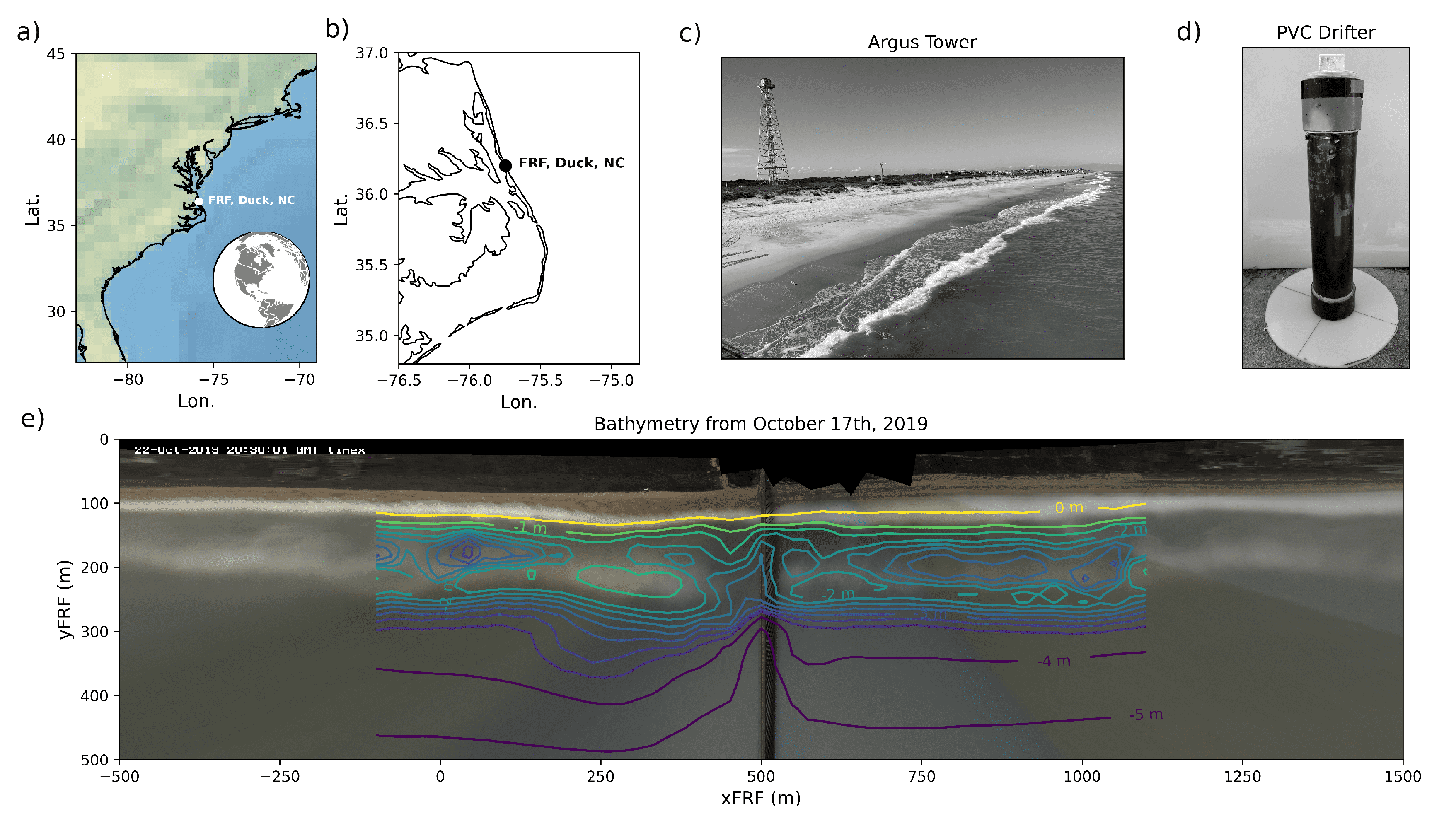
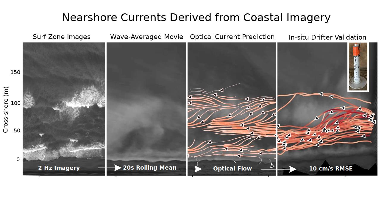
Coastal imagery used in this study was acquired from the U.S. Army Corps of Engineers’ (USACE) Field Research Facility (FRF) in Duck, NC, USA (described in Section 2.1, Figure 1). Section 2.2 presents WAMFlow, a methodology based on a concept previously applied to X-band radar observations [23] and coastal shelf imagery to identify internal waves [24]. A rolling temporal average of movie frames was used to remove the surface waves and associated foam organization not coherent with mean flow patterns. These wave-average movies (WAMs) were then processed with a common, efficient dense optical flow technique to derive flow patterns with components in both the along- and cross-shore directions (details in Section 2.3).

2.1. Field Site

The FRF shoreline is oriented −18.2° north-northwest of true north, composed of ∼0.2 mm mean grain size sand on a foreshore of 1:12.5 with one to two sandbars typically present [25]. The FRF site is an active field observatory where beach topography and nearshore bathymetry data are collected at monthly intervals. In situ hydrodynamic gauges are deployed within or outside the surf zone providing nearly continuous, point-based data streams of wave spectra, currents, and tides. Remote optical observations of the surf zone are also made nearly continuously during daylight hours from a 6-camera array mounted on top of a 43 m high tower (known as the Argus Tower, [26]). Ocean wave characteristics are measured by a directional pressure array in 8 m of water immediately offshore of the Argus Tower [27]. Water levels, including semi-diurnal tides and non-tidal residuals are recorded at the National Ocean and Atmospheric Association’s Station 8651370, located at the end of the FRF pier.

Beyond the operational measurements, additional targeted field measurements were made coinciding with the During Nearshore Event Experiment (DUNEX) pilot study carried out in Fall 2019 at the FRF. Bathymetric surveys were periodically obtained during DUNEX (representative survey from 17 October 2019 immediately offshore of the Argus Tower provided in Figure 1e), identifying a single sandbar in −3 m of water depth and approximately 100 m offshore. The coordinate system presented in Figure 1e is a local reference field particular to the cross-shore and alongshore axes of the FRF shoreline. The origin is located at the southern edge of the property (36.1776°N, 75.7497°S), with the y-axis oriented alongshore such that increasing yFRF corresponds to more northerly portions of the beach while increasing xFRF corresponds to distance from the dunes and thus deeper water.

2.2. Data Acquisition

The Argus station is composed of six separate high-resolution optical cameras [26]. This particular platform has been in operation since 1986 (with the present cameras in operation since 2015) and has been utilized in many studies during the last four decades, including sandbar tracking [25], shoreline variability assessments [28], and the development of bathymetric inversion techniques [29]. Each camera records 2048 × 2448 pixel images at 2 Hz for 17 min beginning every half hour (during daylight), which generates a total of >60 GB of data per half hour recording. Typically, the images are postprocessed to a set of standard products rather than saving the raw images, greatly reducing the necessary data storage and enabling continuous monitoring [30]. For this study, a limited number of complete full-frame raw image recordings were saved during drifter deployments and processed following the steps outlined in Figure 2.

Raw images were converted from 3-bands (RGB) to grayscale and rectified to 1 m by 1 m grid in local FRF coordinates using open-source software (Python interface to OpenCV [31]) and by assuming the vertical location of the water surface to be the observed tide height. Co-incident images from all six cameras were then merged to create single frames with spatial coverage of 2 km in the alongshore and 0.5 km in the cross-shore (same spatial coverage as Figure 1e: xFRF = −500 m to 1500 m and yFRF = 0 m to 500 m). Exposure was not postprocessed to match across all cameras or across all merged images (i.e., varying brightness due to passing cloud cover), and no image processing was performed to enhance image texture. Wave-averaged movies were created by a running average time window of twice the dominant wave period measured at the 8 m array to ensure about two individual wave breakers and passing bore fronts were included in each average. A time-step between frames of 5 s was then used to reduce movie file size and increase perceived motion of residual foam between frames. The effect of these user decisions are discussed further in Section 4. 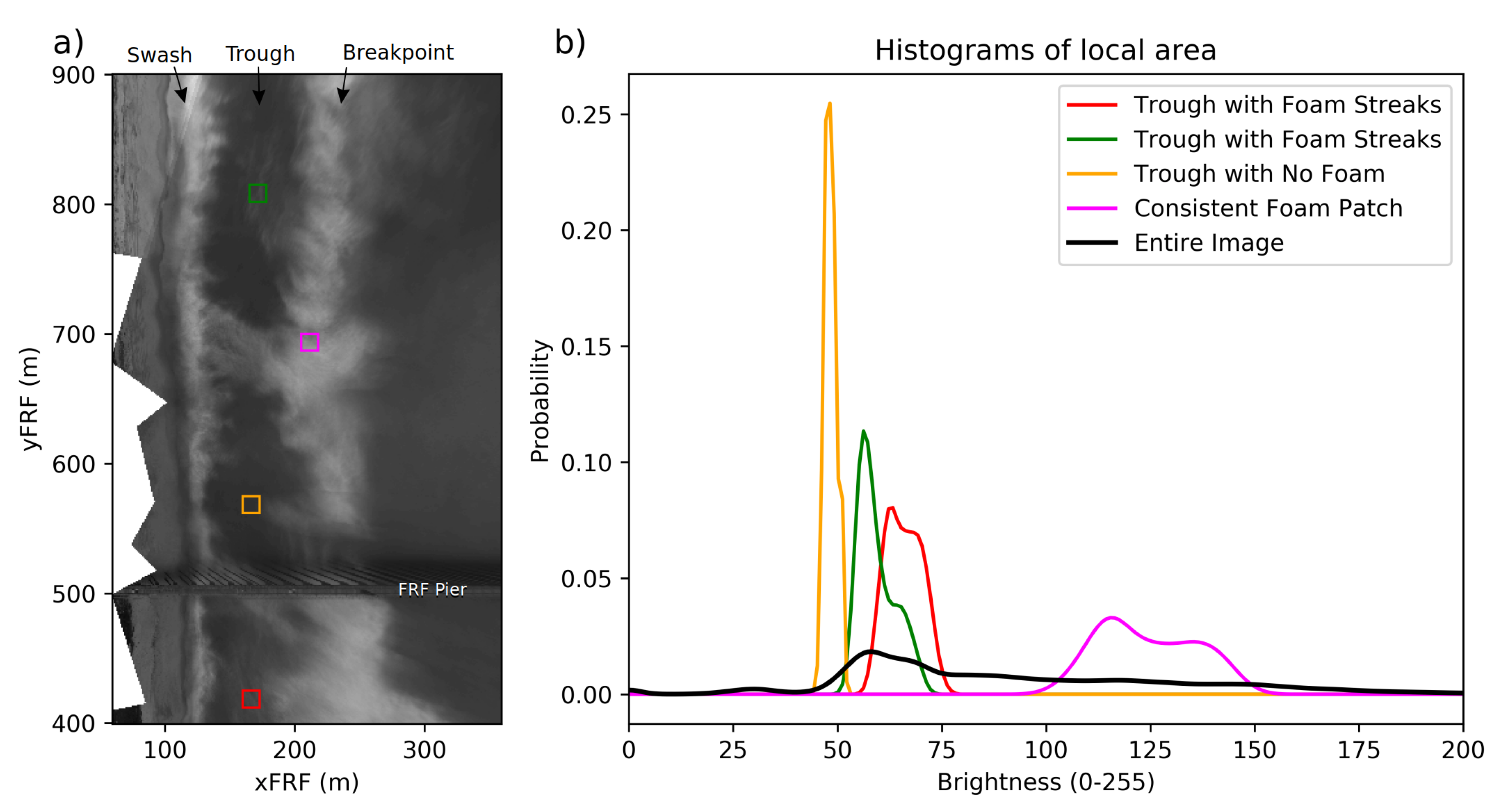An example frame from a WAM computed using this technique is shown in Figure 3a. The image reveals where consistent wave breaking occurs by emphasizing regions of greater reflectance. In this example, higher foam generation occurs at the sandbar breakpoint (xFRF = 180 m) and in the swash zone (xFRF = 125 m). Although the product is comparable to the traditional timex (10 min averages, e.g., [32]), the much shorter temporal window retains more ephemeral residual foam streaks. Foam streaks are observed in Figure 3a in the sandbar trough (region with less breaking between xFRF = 125–180 m) and immediately north of the FRF pier due to flow separation around pilings.

2.3. Optical Flow Estimates

Computer vision technology has rapidly advanced over the last few decades, largely motivated by automation needs unrelated to oceanographic research. However, adaptation and leveraging of these emerging technologies has the potential to greatly enhance surf zone research. In this work, the application of a dense optical flow algorithm is explored to evaluate its ability to track the advecting foam patterns visible in WAMs. Numerous approaches have been developed to close the generic optical flow assumption that brightness is conserved:

$$\frac{\partial I}{\partial x}{U}_x+\frac{\partial I}{\partial y}{U}_y+\frac{\partial I}{\partial t}=0$$

(1)

where I is the image intensity, U is the apparent velocity, x and y are image dimensions, t is time, and subscripts denote vector components. This study uses a polynomial expansion to identify gradients of consecutive images’ intensities [33,34] (code freely available in OpenCV). The selected method closes the number of equations to a number of unknowns by assuming that the displacement field is slowly varying such that information can be integrated over a local neighborhood (user decision). The number of previous frames to consider and an option to provide an initial flow field guess are additional user decisions not explored in this work. Velocities are ultimately derived at every pixel and every time step throughout the entire video.

2.4. Filtering Optical Flow Results

Similar to previous efforts estimating nearshore velocities, the resulting flow fields from this method contain noise in both space and time as a consequence of both natural processes and the wave-averaged image processing technique. Often the most common factor decreasing signal to noise ratios in optical tracking algorithms is the introduction of new targets and/or disappearance of old targets. In this application, “targets” are locally bright pixels relative to the background brightness (i.e., bright white foam against dark water). When targets are not consistently present, the basic assumption that image pixels can be correlated between subsequent frames or that intensities/gradients are congruent between frames is fundamentally broken. This potential error source becomes particularly relevant for WAMs: the spatial and temporal resolution reduction which aims to minimize the presence of wave and turbulence also effectively increases the percentage of frames with new targets present.

This issue has previously been addressed with high frame rates that reduce the ratio of frames with target discontinuties to frames with consistent targets [15,16]. Introduction and decay of tracers has also been accounted for in scenarios where the user systematically introduces targets by defined input functions with decay terms (i.e., periodic inputs of a specific magnitude with a known exponential decay rate of the tracer presence [35]). However wave breaking is a chaotic, quasi-random process and the persistence of foam in the surf zone exhibits dependencies on the kind of wave breaking, water temperature, and biological/chemical content [36], necessitating more research focused on these dynamics before properly constraining such functions in the present problem. Discontinuities in target presence are accounted for in this study by postprocessing with two metrics specifically related to elements of the WAM video prior to applying optical flow; large changes in mean local brightness, and low local brightness standard deviation. The metrics are efficiently obtained over the same size pixel area as the optical gradient calculation by applying 5 × 5 pixel convolution filters to every image in the WAM. When considering the distributions for brightness obtained in each local area, regions with no surface tracers result in narrow, peaked distributions (low standard deviation) and low means (note yellow distribution in Figure 3b), while regions with surface foam exhibit wider distributions (high standard deviation) and high means (Figure 3b).

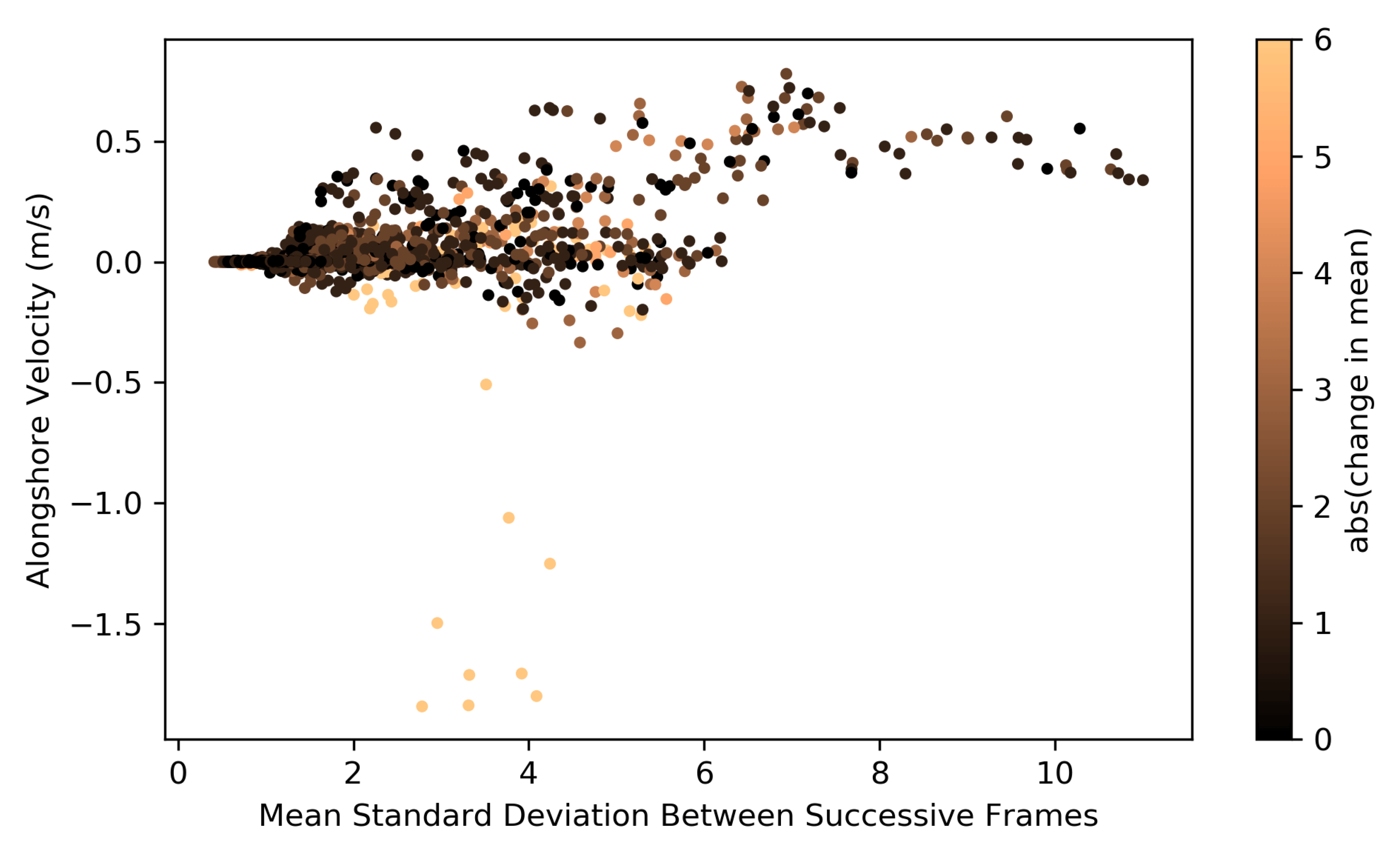
Alongshore velocity estimates from an example region (green box in Figure 3a) in the trough between the shoreline and sandbar are shown in Figure 4 to highlight several trends between local intensity distributions and predicted velocities. Distributions with large changes in the local mean between successive frames can result in anomalous large velocities (note that the relatively rare large positive velocities all occur with large frame-to-frame changes in brightness). Local brightness changes greater than 5 are thus considered as a proxy for the introduction or disappearance of targets, and all such returns are removed in postprocessing. Low local standard deviations also consistently result in optical flow returns of zero velocity, indicating that foam tracers were not present but not necessarily ruling out that water was not flowing at that time. All velocity estimates occurring during instances of standard deviations less than 2 are discarded as potentially poor estimates due to not adhering to the underlying assumptions of the optical flow algorithm.

3. Results: Comparison to In Situ Observations

Drifters were deployed in the nearshore on three different days during DUNEX with varying degrees of wave height, period, and direction relative to shore normal (

Table 1. Environmental conditions for the three drifter deployments and image recordings.

Date	Time Released	Number Deployed	Hs (m)	Tp (s)	Dir (Deg from Normal)	Tide Stage	Water Level Range (m)	Wind Mag. (m/s)	Wind Dir. (N)
10/22/19	13:20	15	0.9	8	−3	Flooding	−0.14 to 0.45	3.3	121
10/30/19	14:05	9	1.6	11	1	Ebbing	0.9 to 0.5	5.2	55
10/31/19	15:15	34	1.4	12	−13	Ebbing	0.82 to −0.12	7.4	178

). Each deployment contains enough tracks to discern flow patterns both within and outside of the breaker zone, capturing longshore currents, rip ejections, and circulation cells within the surf zone. Each drifter was 60 cm in length, 10 cm in width, and composed of PVC piping with water tight fittings, which follows a now common surf zone drifter design used at sites around the world [37,38,39,40] (Figure 1d). GPS and IMU sensors were located at the top of the drifter with a cellular modem communicating its location in real-time back to shore personnel while also saving data to the cloud to prevent data loss if a drifter was damaged and flooded in the shore break. Buoyancy was adjusted to maintain near-consistent satellite signals and cell network reception (5–10 cm of the drifter piercing the surface). Drifters were deployed by dropping them in the water from the FRF pier at varying cross-shore locations and by collecting them after they had freely floated to shore and washed up in the shore break. Deployments lasted from one to three hours, each containing varying temporal and spatial coverage due to variability in drifter path, i.e., some drifters slowly meandered while others rapidly moved kilometers away from the FRF property during deployments with strong longshore currents. Drifters intermittently lost satellite and/or cell service due to submergence onshore of breaking waves; however, lost connections were rarely longer than 1–2 s and previous efforts have found reasonable results using linear interpolation to fill the data gaps [41,42]. Raw GPS returns were processed following the techniques of MacMahan et al. [37].

3.1. Spatial Velocity Patterns

Surf-zone currents derived with WAMFlow from 17 min WAMs are compared side by side with drifter deployments in Figure 5, Figure 6 and Figure 7. Estimated currents are temporally averaged velocities from the entire 17 min image recordings after removing returns identified by the steps discussed in Section 2. Remotely sensed circulation patterns are presented as stream plots to facilitate comparison to in situ observations. Stream plots essentially highlight the expected flow paths that a drifter would follow if it were dropped anywhere within the remotely sensed domain. Note, however, that drifter deployments all occurred over time periods longer than 17 min and, thus, the derived WAM pattern may not have observed the specific conditions drifters experienced.

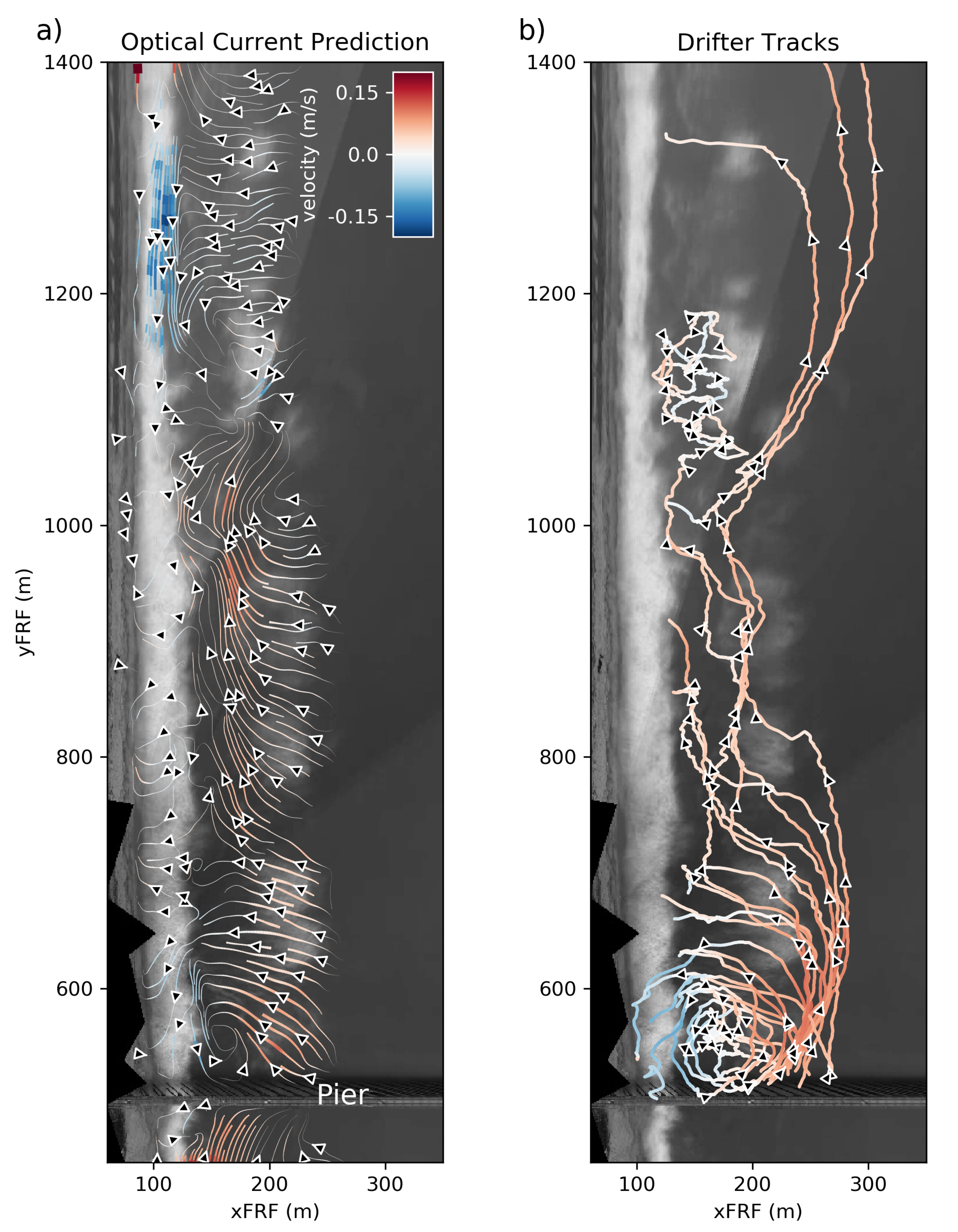
The time-averaged current prediction for 22 October 2019 at 15:30 (UTC) identifies a counter-clockwise gyre adjacent to the pier on similar alongshore length scales to the drifter behavior (Figure 5). Predominantly positive alongshore velocities are also remotely sensed between yFRF = 700 m and 1100 m, where drifters consistently propagated in the alongshore within the trough between the sandbar and the shore break (Figure 5). A convergence point is identified at yFRF = 1100 m and xFRF = 175 m, right in the vicinity of a stagnation point for a drifter, which consistently stayed within a 120 m × 60 m box for over an hour before being retrieved at the end of the deployment. Three drifters where ejected from the surf zone at yFRF = 1050 m, which is the only alongshore location within the optical current estimates where stream flow trajectories are pointed in the offshore direction at the outer edge of the surf zone.

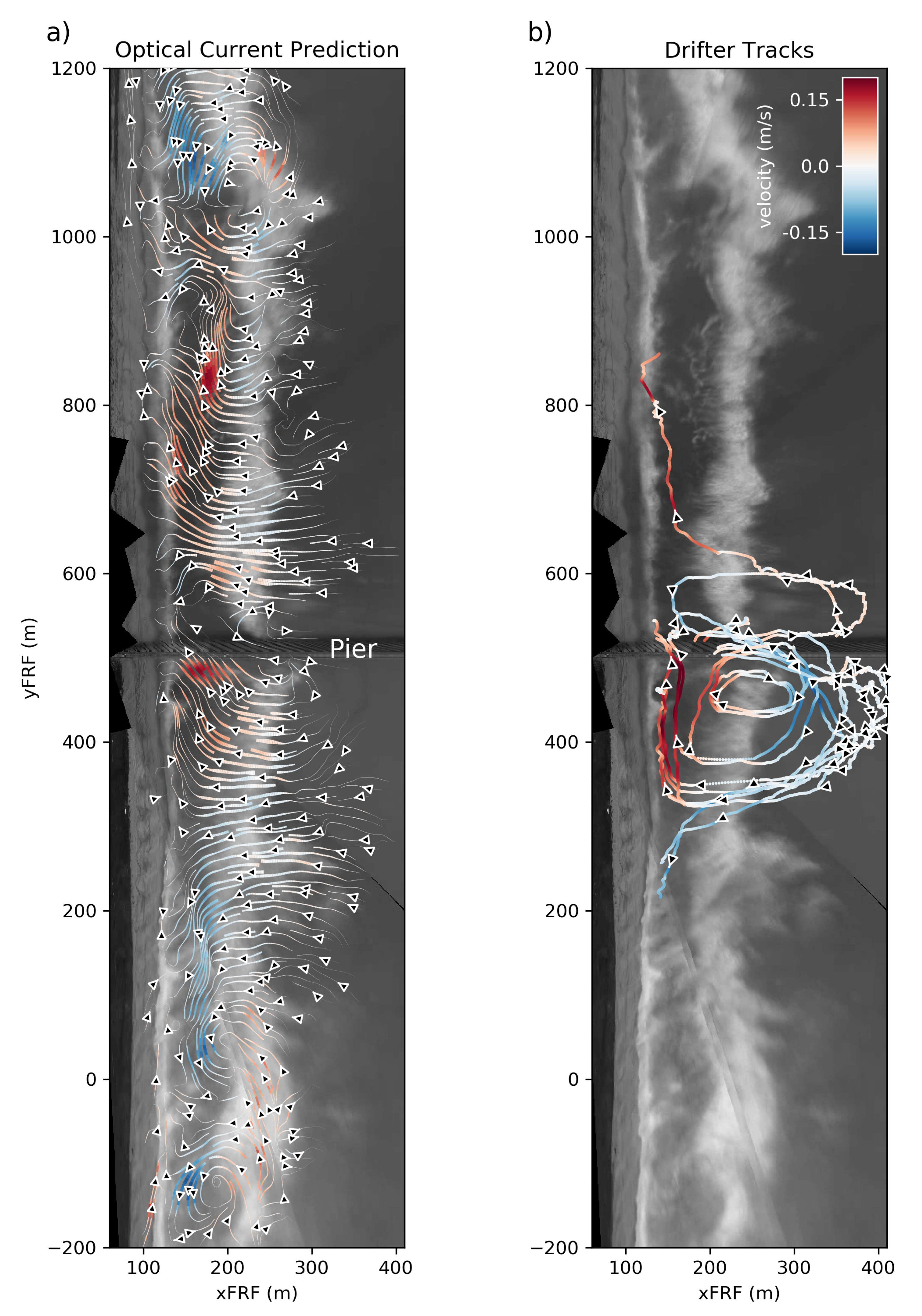
Offshore directed stream trajectories are also resolved in the remotely sensed velocities for 30 October 2019 at 14:00 (Figure 6) at a slight angle from north to south underneath the pier as well as at approximately equal alongshore distances away from the pier at yFRF = −100 m and yFRF = 1050 m. The angled rip under the pier matches the offshore trajectories of all of the drifters dropped into the water from the pier. After the drifters were ejected from the surf zone, they spent as long as 45 min in a region, where the optical estimates did not resolve velocities (outside of xFRF = 350 m between approximately yFRF = 400–500 m) but subsequently drifted back onshore across the sandbar and entered stronger alongshore flows in the trough. Divergences of alongshore flows at yFRF = 300 m and yFRF = 600 m are resolved in both the drifter trajectories and optical velocity estimates. Although the drifters rarely escaped the reciruclation cells north and south of the pier, the broader remotely sensed field highlights that the divergences in the trough are a consequence of feeder currents due to multiple rip currents in the domain.

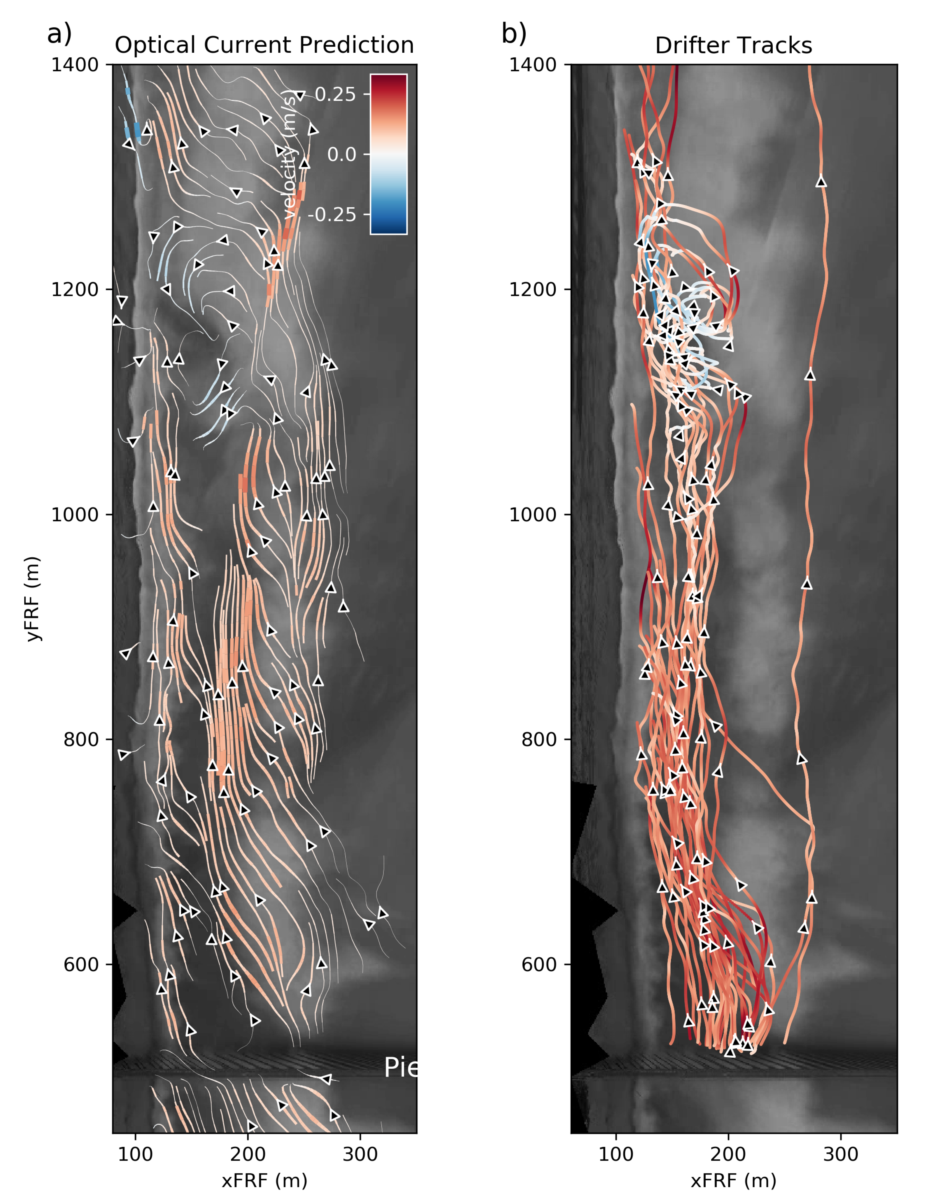
Velocity estimates for 31 October 2019 at 17:00 further highlight that the method is capable of resolving complicated flow patterns inside of the breaker line (Figure 7). Northward-directed longshore flows are resolved between the FRF pier and yFRF = 1100 m. Adjacent counter-rotating gyres are identified between yFRF = 1100–1300 m, in the same location that the drifters experienced a complicated recirculation before continuing in the alongshore. This particular WAM also reveals how the pattern returned is dependent on the assumption that the surf zone is saturated with residual foam. In this example, foam produced by the outer breaker is swept off in a swift longshore current before saturating the entire trough, resulting in few optical current solutions between xFRF = 150–200 m. Note that drifter tracks through this region show strong alongshore flows, highlighting the potential for false negatives from the optical flow measurements. However, in this case, our filtering mechanism correctly removes low confidence optical flow estimates in this region. Similarly, the deeper water under the pier results in less depth-limited breaking and less foam generation such that immediately 50 m north of the pier has less residual foam to track despite drifters in that region consistently being swept north at similar speeds to the rest of the surf zone.

Each of the drifter deployments in Figure 5, Figure 6 and Figure 7 contain unique spatially varying behavior to assess the validity of WAM-derived surface currents. The optical flow algorithm clearly resolves 2D patterns spatially coherent with drifter tracks entrained in longshore currents, rip currents, gyres, and large recirculation cells. The similarities between flow field attributes and drifter behavior are striking. Even in regions devoid of drifter tracks, the remotely sensed product provides context for why drifters did not enter that region. For example, the stagnated drifter at yFRF = 1100 m in Figure 5b is likely due to the southward directed currents resolved by the WAM between yFRF = 1100 and 1300. Similarly, the drifter tracks in Figure 6b that end at yFRF = 200 m and yFRF = 900 m appear to be the due to convergences resolved in the remotely sensed pattern. It is noteworthy that the 1 m × 1 m pixel-sized WAMs capture both localized flow features on the scale of 10 s of meters and large-scale patterns on the scale of 100 of meters without any need for adaptive resolutions.

3.2. Velocity Magnitude Comparison

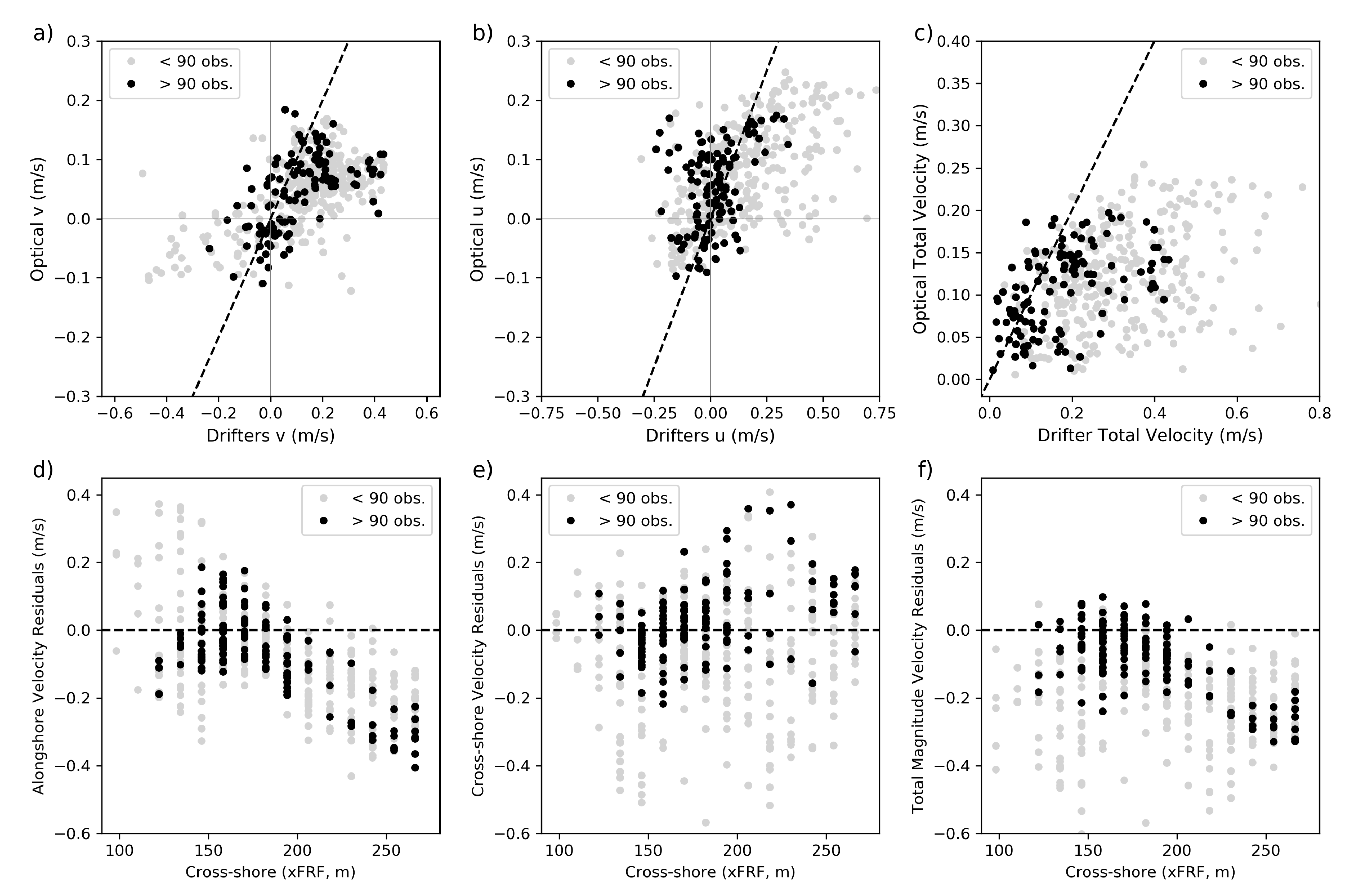
Figure 8 presents a velocity magnitude comparison for 22 October. Of the three days presented in Section 3.1, this deployment included the greatest number of drifter tracks occurring within the shortest amount of time and co-incident with a WAM movie recording. Limiting the time-window of comparison to only while cameras were collecting reduced the drifter dataset by >75%; thus, it is assumed that the mean current patterns was consistent throughout the deployment. All observations during the drifter deployment were binned into a 15 m × 15 m grid regardless of time and averaged to obtain flow vectors. Optical flow current estimates were binned to the same grid to facilitate one-to-one comparisons (Figure 8). Scatter within the one-to-one plots exhibits a correlation with respect to both cross-shore location and the number of drifter observations within each bin, suggesting that extremes are largely to blame for high error metrics (Figure 8a–c). For example, if all alongshore velocities of the optical current are considered, then that results are biased lower relative to drifters by 40% and root mean square error (RMSE) of the total velocity magnitude is 0.22 m/s (Figure 8a). However, longshore optical currents are consistently lower in magnitude relative to drifters outside of the surf zone (points greater than xFRF = 210 m in Figure 8d–f), where trackable features such as residual foam are infrequent and optical flow often predicts zero velocities. Optical predictions also have greater residuals in the inner most portion of the surf zone; however, the large drifter velocities in this region reflect a higher frequency of drifters surfing waves due to the relatively shallower water depths and plunging breakers being the shore. The in situ drifter measurements considered as “truth” in this validation are thus unlikely a reflection of wave-averaged processes outside of the surf zone (points greater than xFRF= 200 m in Figure 8d–f) and in the most inner portion of the surf zone (points less than xFRF = 150 m in Figure 8d–f).

Velocity predictions from the middle of the surf (xFRF = 130–210 m) exhibit an alongshore RMSE of 0.15 m/s and a cross-shore RMSE of 0.13 m/s. Ultimately, the one-to-one comparison of wave-averaged processes is dependent on the degree to which the drifter measurements are truly representative of wave-averaged motions. More observations within a particular 15 m × 15 m grid cell result in a higher likelihood that the average is representative of mean flow, while bins with fewer observations tend to have greater discrepancies (Figure 8d–f). Focusing on only those points with more observations (black dots) notably reduces the spread of the residuals. RMSE of only those total velocity magnitudes in the trough with more than 90 observations within the bin is 0.10 m/s (Figure 8f).

4. Discussion

4.1. Limitations and Future Improvements

The method presented in this work demonstrates that two-dimensional nearshore current patterns can be derived by reducing optical clutter prior to applying a tracking algorithm. However, future work investigating the performance of WAMFlow in a range of conditions with additional in situ observations could further develop the presented filtering techniques, potentially improving results presented in this study. For example, high winds will likely yield some surface wind drift on the surface foam field. As these apparent wind-driven flows will deviate form the near-surface water flows that are of primary interest using this method, the effect of winds can ideally be identified and calibrated for with a longer time window of field observations, similar to the previous methods of Chickadel et al. [13]. Optimizing user decisions for the window of temporal averaging and the time-step between frames would similarly benefit from a field effort with fixed instruments. The chosen parameters in this study were decided on after attempting to generate WAMs at a range of different time scales. Averaging windows shorter than two wave periods contained greater wave-associated noise and often contained a perceptible bore front that downscales to optical flow predictions of predominantly onshore-directed currents. Longer averaging windows resulted in smeared residual foam over a larger area, which can result in zero velocity returns along the middle stretches of particularly long foam streaks. Zero velocity returns can be produced across the entire surf zone if the time window is long enough to encompass both target generation (wave breaking bubble formation) and target loss (bubble dissipation). This suggests that the user decision of window length may be a function of underlying biogeochemical water properties that facilitate longer residual foam lifetimes and thus fewer lost targets creating noise in tracking algorithms [43].

The chosen optical tracking algorithm could also be improved in future developments of WAMFlow. The algorithm used is relatively simple and computationally fast compared to the latest optical flow techniques, which incorporate machine learning methods such as convolutional neural networks and are often tailored to specific applications (i.e., identifying individual high velocity objects [44], and identifying and removing rain streaks [45]). A common critique of the optical flow formulation used in this work is that the underlying assumptions result in a smooth velocity field as opposed to identifying sharp edges of individual objects. This critique is relevant in unprojected videos that retain 3-dimensional depth within each frame, particularly when multiple objects move at different distances relative to the camera, such that the apparent flow field should contain discontinuities at object edges [46]. The WAMs analyzed here are derived from rectified imagery on flat planes (depth-corrected), composed of features with blurred edges such that no object segmentation is required. The application is also intended to resolve a smoothly varying wave-averaged natural process that does not require resolving discontinuities in nearshore flow fields. Thus, the enhanced capabilities of the more complex/cutting-edge algorithms are in fact less desirable in this application.

The error metrics reported in this work assume that drifter observations correctly characterize the surf zone flows. However, direct comparison of drifter velocities to either remotely sensed currents or stationary in situ current meters is a notably difficult problem [20,37,42]. The drifters are immersed in the flow such that they experience individual wave-by-wave motions. Despite the drifters including features to dampen wave-by-wave responses, the momentum generated by wave breaking can still result in drifter movements that are unrepresentative of wave-averaged motions. Transient flow structures on the order of only a few minutes or less, such as eddies resulting from localized wave-breaking induced vorticity or shearing on the edge of longshore currents, can also cause a drifter to experience a flow magnitude and direction that are different from what the global time averaged flow would otherwise be for a particular location. In the case of the field observations presented in this study, further complications arise from the drifter deployments occurring over longer periods of time than the image recordings. The longer a drifter deployment, the greater the likelihood that changes in environment conditions such as tide level and offshore waves could result in different spatial current patterns in the surf zone.

4.2. Comparison to Other Remote Sensing Analyses

Longterm monitoring of remotely sensed alongshore currents is typically performed with timestack approaches [13,14]. The same select line of alongshore-oriented pixels is saved from multiple frames to significantly reduce necessary data storage. The alongshore orientation filters out breaking waves as purely horizontal streaks in the timestack, which is an alternate approach for removing the wave-induced optical clutter in the nearshore. Unfortunately, the assumptions of such methods prevent the derivation of cross-shore flow components. Gyres, recirculating eddies, and rip currents are all undetected. Recent work has suggested that such cross-shore features can still be inferred by assimilating multiple remotely sensed products or assuming continuity to infer cross-shore components [47,48]. Previous attempts to resolve two-dimensional patterns using optical methods have necessitated high resolutions and high frame rates, which prevents longterm, continuous monitoring due to computational effort ([20]). By comparison, the 2 km by 0.5 km domain in this work results in wave-averaged movies of 15 to 60 mb for file sizes ranging from timesteps of 2 to 10 s. The open-source codes utilizing C, C⁺⁺, and Python languages can compute a 30 mb file in about 20 s with serial processing. The 1 × 1 m meter pixel size chosen in this study is also a relatively low resolution, suggesting both that meaningful results could be obtained from low-cost monitoring stations (surf and beach cams) and that larger domains or increased resolutions could be investigated without the WAMFlow becoming computationally excessive.

4.3. Potential for New Insights on Surf Zone Current Patterns

Quantified spatially and temporally varying current fields on the scales presented in this work have the potential for providing new insights on fundamental surf zone dynamics not readily obtainable with previous in situ gauge data or remote sensing products. The unique combination of continuous monitoring during daylight hours at large spatial extents has the potential to illuminate variability on temporal scales ranging from hourly wave and water level changes to feedback-induced flow evolving during morphologic beach state progressions occurring on the order of weeks to seasons.

4.3.1. Relevance of Environmental Conditions Governing Patterns

An illustrative example of the ability to capture short-term temporal variability is provided in Figure 9, where WAMs were obtained for high tide (10:30) and low tide (17:00) on 31 October 2019. Consistent alongshore flows to the north were present in the sandbar trough while mean water levels were elevated at high tide and wave angles approached from 13 degrees south of shore-normal. The surf zone extent was less than 150 m, with intermittent breaking on the sandbar and a swash zone noticeable in the timex (Figure 9a). Flow patterns inside of the breaker line transitioned to include a two-dimensional recirculating gyre near yFRF = 1200 m as the mean water level approached low tide despite offshore wave conditions holding steady (Figure 9b). The intensity of wave breaking on the sandbar became amplified, the swash zone contained less energy, and the surf zone was relatively wider. This suggests that, although general surf zone assumptions would indicate a strong alongshore flow due to the steeply approaching offshore waves, the tidal level and associated morphologic configuration were more important factors controlling the mean current pattern. Such insights are not necessarily new; veloocity observations from sparsely distributed fixed instruments have provided enough context to identify a correlation between diurnal tidal fluctuations and the intensity of nearshore circulation associated with more intense wave breaking, e.g., [49]). Predictive models for rip currents have also identified low tidal levels as statistically significant predictors of more intense flows [50]. However, this example demonstrates that WAMs are capable of providing much greater two-dimensional spatial context compared to the fixed arrays, and if operational for long enough time periods, WAMs could be invaluable for quantifying relative importance and thresholds above or below which each environmental condition or morphologic configuration becomes the dominant factor governing nearshore flow patterns.

4.3.2. Timescales and Frequency of Intermittent or Transient Features

The wave-averaged returns also have considerable potential with respect to shorter-term flow field variability (i.e., motions occurring on the order of minutes within a WAM). Figure 10a–c are example flow maps for shorter two minute averages of optical flow returns occurring within a WAM recorded on 11 September 2019. No drifter tracks are available for ground truth on this day, but the WAM contains a variety of notable behaviors demonstrating intriguing applications to which WAMs could contribute insight. Normally, incident waves with $H_s$ of 0.8 m at 11 s consistently break on the sandbar, forming cresentic shapes in the timex but with occasional “holes” in the alongshore. The underlying morphology at this time contained a number of cresentic sandbars with horns located in relatively shallow water close to the shoreline compared to adjacent tips in deeper waters slightly further from the shoreline.

Figure 10d provides the alongshore variation of averaged cross-shore currents at all points offshore of xFRF = 200 m for each snap shot from the WAM. Onshore-directed velocities dominate the outer surf zone of the 1 km domain; however, localized regions of offshore-directed flows are also apparent. Such regions are interpreted here as indicative of rip currents with varying widths and intensities. Rip currents can be persistent features occurring where feedback generated a channel within the sandbar and can be intermittent or transient features. Considerable research has been devoted to both varieties in support of the societal need for rip warnings, but the responsibility to identify such features still largely falls on human eyes and fundamental questions regarding forcing, persistence, and spatial scales are still active research areas [51]. Figure 6 highlighted the ability to detect a persistent rip current underneath the FRF pier, which is similarly present in Figure 10d. However, the shorter time averages reveal intermittent rip currents on the southern side of the pier between yFRF = 0–100 m and on the northern side of the pier between yFRF = 800–850 m. Both rips occur at holes between crescentic bars; however, the northern rip was only detected for a 5 min duration while the southern rip was present for nearly 14 min. The southern rip also exhibited temporal variability in intensity, width, and detected distance outside of the surf zone, suggesting that an extended dataset of WAMs could identify the variability of such rip attributes and potential correlations with environmental conditions.

Several locations with transient eddies on the order of 10 s of meters can also be identified throughout the frames (orange rectangles). These include instances adjacent to the pier rip current which may be shearing of the offshore directed flows by onshore-directed wave breaking momentum in the adjacent shallow bar regions (Figure 10b). Eddies are also identified within the trough where alongshore flows potentially experience shear instabilities (Figure 10a). Transient eddies are also detected in the trough regions immediately onshore and slightly offset from shallowest sandbar horns, where vorticity is injected by local finite length-scale wave crests experiencing locally varying shoaling and refraction. The relevance of such rotational flows to low-frequency motions, energy dissipation, and mixing in the surf zone is an active research topic [5,9,10].

5. Conclusions

The nearshore current patterns presented in this study suggest that the reduction of visual clutter by wave-averaging images of the surf zone is a viable method for deriving underlying fluid motions. WAMFlow, a global optical flow algorithm coupled with filtering to remove velocity estimates associated with pixels that break underlying object tracking assumptions (target appearance/disappearance), was shown to produce nearshore circulation patterns consistent with in situ drifter deployments. Velocity residuals within the trough exhibited an RMSE of 10 cm/s, but it is noteworthy that the in situ drifter velocities are not a true representation of mean currents. Quantifying true errors with respect to wave-averaged motions will necessitate a larger field program with fixed current meters. Alongshore flows focused within sandbar troughs, persistent circulation cells contained entirely within the surf zone, and large recirculations exciting the surf zone are resolved with the two-dimensional approach presented in this study. Local-scale transient eddies and intermittent rip currents were also identified within processed WAMs, suggesting the presented methodology has the potential to advance both fundamental understandings of surf zone hydrodynamics and practical applications for surf zone observations.

References

1. Radermacher, M.; de Schipper, M.; Reniers, A. Sensitivity of rip current forecasts to errors in remotely-sensed bathymetry. Coast. Eng. 2018, 135, 66–76. [Google Scholar] [CrossRef] [Green Version]
2. Rodriguez, A.; Giddings, S.; Kumar, N. Impacts of Nearshore Wave-Current Interaction on Transport and Mixing of Small-Scale Buoyant Plumes. Geophys. Res. Lett. 2018, 45, 8379–8389. [Google Scholar] [CrossRef] [Green Version]
3. Roelvink, J. Coastal morphodynamic evolution techniques. Coast. Eng. 2006, 52, 277–287. [Google Scholar] [CrossRef]
4. Longuet-Higgins, M.; Stewart, R. Radiation stress and mass transport in gravity waves, with application to ‘surf beats’. J. Fluid Mech. 1962, 13, 481–504. [Google Scholar] [CrossRef]
5. Elgar, S.; Raubenheimer, B. Field Evidence of Inverse Energy Cascades in the Surfzone. J. Phys. Oceanogr. 2020, 50, 2315–2321. [Google Scholar] [CrossRef]
6. Reniers, A.; Thornton, E.B.; Stanton, T.P.; Roelvink, J. Vertical flow structure during Sandy Duck: Observations and modeling. Coast. Eng. 2004, 51, 237–260. [Google Scholar] [CrossRef]
7. Haller, M.C.; Honegger, D.A.; Catalan, P.A. Rip Current Observations via Marine Radar. J. Waterw. Port Coast. Ocean. Eng. 2014, 140. [Google Scholar] [CrossRef] [Green Version]
8. Craik, A.; Leibovich, S. A rational model for Langmuir. J. Fluid Mech. 1976, 73, 401–426. [Google Scholar] [CrossRef] [Green Version]
9. Kirby, J. Recent advances in nearshore wave, circulation, and sediment transport modeling. J. Mar. Res. 2017, 75, 263–300. [Google Scholar] [CrossRef]
10. Feddersen, F. The generation of surfzone eddies in a strong alongshore current. J. Phys. Oceanogr. 2014, 44, 600–617. [Google Scholar] [CrossRef] [Green Version]
11. Holman, R.; Haller, M. Remote sensing of the nearshore. Annu. Rev. Mar. Sci. 2013, 5, 95–113. [Google Scholar] [CrossRef] [Green Version]
12. Shen, C.; Huang, W.; Gill, E.W.; Carrasco, R.; Horstmann, J. An algorithm for surface current retrieval from X-band marine rader images. Remote Sens. 2015, 7, 7753–7767. [Google Scholar] [CrossRef] [Green Version]
13. Chickadel, C.; Holman, R.; Freilich, M. An optical technique for the measurement of longshore currents. J. Geophys. Res. 2003, 118. [Google Scholar] [CrossRef] [Green Version]
14. Almar, R.; Larnier, S.; Castelle, B.; Scott, T.; Floc’h, F. On the use of the Radon transform to estimate longshore currents from video imagery. Coast. Eng. 2016, 114, 301–308. [Google Scholar] [CrossRef] [Green Version]
15. Holland, K.T.; Puleo, J.A.; Kooney, T.N. Quantification of swash flows using video-based particle image velocimetry. Coast. Eng. 2001, 44, 65–77. [Google Scholar] [CrossRef]
16. Puleo, J.A.; Farquharson, G.; Frasier, S.J.; Holland, K.T. Comparison of optical and radar measurements of surf and swash zone velocity fields. J. Geophys. Res. 2003, 108. [Google Scholar] [CrossRef]
17. Perkovic, D.; Lippmann, T.C.; Frasier, S.J. Longshore Surface Currents Measured by Doppler Radar and Video PIV Techniques. IEEE Trans. Geosci. Remote Sens. 2009, 47, 2787–2800. [Google Scholar] [CrossRef]
18. Rivillas-Ospina, G.; Pedrozo-Acuna, A.; Silva, R.; Torres-Freyermuth, A.; Gutierrez, C. Estimation of the velcoity field induced by plunging breakers in the surf and swash zones. Exp. Fluids 2012, 52, 53–68. [Google Scholar] [CrossRef]
19. Chickadel, C.C.; Horner-Devine, A.R.; Talke, S.A.; Jessup, A.T. Vertical boil propagation from a submerged estuarine sill. Geophys. Res. Lett. 2009, 36. [Google Scholar] [CrossRef] [Green Version]
20. Derian, P.; Almar, R. Wavelet-Based Optical Flow Estimation of Instant Surface Currents From Shore-Based and UAV Videos. IEEE Trans. Geosci. Remote Sens. 2017, 55, 5790–5797. [Google Scholar] [CrossRef]
21. Thorpe, S.A.; Smith, W.A.M.N.; Thurnherr, A.M.; Walters, N.J. Patterns in foam. Weather 1999, 54, 327–334. [Google Scholar] [CrossRef]
22. Benbow, C.A.; MacMahan, J.H.; Thornton, E.B. Analysis of Surface Foam Holes Associated with Depth-Limited Breaking. J. Coast. Res. 2017, 33, 1271–1282. [Google Scholar] [CrossRef]
23. Honegger, D.A.; Haller, M.C.; Geyer, W.R.; Farquharson, G. Oblique Internal Hydraulic Jumps at a Stratified Estuary Mouth. J. Phys. Oceanogr. 2017, 47, 85–100. [Google Scholar] [CrossRef]
24. Suanda, S.H.; Barth, J.A.; Holman, R.A.; Stanley, J. Shore-Based Video Observations of Nonlinear Internal Waves across the Inner Shelf. J. Atmos. Ocean. Technol. 2014, 31, 714–728. [Google Scholar] [CrossRef]
25. Plant, N.; Holman, R.; Freilich, M.; Birkemeier, W. A simple model for interannual sandbar behavior. J. Geophys. Res. 1999, 104, 15755–15776. [Google Scholar] [CrossRef]
26. Holman, R.; Stanley, J. The history and technical capabilities of Argus. Coast. Eng. 2007, 54, 477–491. [Google Scholar] [CrossRef]
27. Long, C.E.; Oltman-Shay, J.M. Directional Characteristics of Waves in Shallow Water; Technical Report Coastal Engineering Research Center; 91-1-1; United States Army Corps of Engineers: Vicksburg, MS, USA, 1991; pp. 1–130. [Google Scholar]
28. Pianca, C.; Holman, R.; Siegle, E. Shoreline variability from days to decades: Results of long-term video imaging. J. Geophys. Res. Ocean. 2015, 102, 2159–2178. [Google Scholar] [CrossRef]
29. Holman, R.; Plant, N.; Holland, T. cBathy: A robust algorithm for estimating nearshore bathymetry. J. Geophys. Res. Ocean. 2013, 118, 2595–2609. [Google Scholar] [CrossRef]
30. Holland, K.; Holman, R.; Lippmann, T.; Stanley, J.; Plant, N. Practical use of video imagery in nearshore oceanographic field studies. IEEE J. Ocean. Eng. 1997, 22, 81–92. [Google Scholar] [CrossRef]
31. Bradski, G. The OpenCV Library. Dobb’s J. Softw. Tools 2000, 3, 1–81. [Google Scholar]
32. Lippmann, T.; Holman, R. The spatial and temporal variability of sand bar morphology. J. Geophys. Res. 1990, 95, 11575–11590. [Google Scholar] [CrossRef]
33. Horn, B.K.; Schunck, B.G. Determining optical flow. Tech. Appl. Image Underst. 1981, 281, 319–331. [Google Scholar] [CrossRef] [Green Version]
34. Farneback, G. Two-Frame Motion Estimation Based on Polynomial Expansion. In Scandinavia Conference on Image Analysis; Springer: Berlin/Heidelberg, Germany, 2003; pp. 363–370. [Google Scholar]
35. Cao, V.; Schaffer, M.; Taherdangkoo, R.; Licha, T. Solute Reactive Tracers for Hydrogeological Applications: A Short Review and Future Projects. Water 2020, 12, 653. [Google Scholar] [CrossRef] [Green Version]
36. Jenkinson, I.R.; Seuront, L.; Ding, H.; Elias, F. Biological modification of mechanical properties of the sea surface microlayer, influencing waves, ripples, foam and air-sea fluxes. Elem. Sci. Anthr. 2018, 6, 1–32. [Google Scholar] [CrossRef] [Green Version]
37. MacMahan, J.; Brown, J.; Thornton, E.B. Low-Cost Handheld Global Positioning System for Measuring Surf-Zone Currents. J. Coast. Res. 2009, 25, 744–754. [Google Scholar] [CrossRef]
38. MacMahan, J.; Brown, J.; Brown, J.; Thornton, E.; Reniers, A.; Stanton, T.; Henriquez, M.; Gallagher, E.; Morrison, J.; Austin, M.J.; et al. Mean Lagrangian flow behavior on an open coast rip-channeled beach: A new perspective. Mar. Geol. 2010, 268, 1–15. [Google Scholar] [CrossRef]
39. Winter, G.; van Dongereen, A.R.; de Schipper, M.A.; van Thiel de Vries, J.S.M. Rip current under obliquely incident wind waves and tidal longshore currents. Coast. Eng. 2014, 89, 106–119. [Google Scholar] [CrossRef]
40. McCarroll, R.J.; Brander, R.W.; Turner, I.L.; Power, H.E.; Mortlock, T.R. Lagrangian observations of circulation on an embayed beach with headland rip currents. Mar. Geol. 2014, 355, 173–188. [Google Scholar] [CrossRef]
41. Johnson, D.; Pattiaratchi, C. A GPS-Tracked Surf Zone Drifter. J. Atmos. Ocean. Technol. 2003, 20, 1069–1075. [Google Scholar] [CrossRef]
42. Johnson, D.; Pattiaratchi, C. Application, modelling and validation of surfzone drifters. Coast. Eng. 2004, 51, 455–471. [Google Scholar] [CrossRef]
43. Callaghan, A.; Deane, G.; Stokes, M.; Ward, B. Observed variation in the decay time of oceanic whitecap foam. J. Geophys. Res. 2012, 117, 1–20. [Google Scholar] [CrossRef] [Green Version]
44. Tu, Z.; Xie, W.; Zhang, D.; Poppe, R.; Veltkamp, R.C.; Li, B.; Yuan, J. A survey of variational and CNN-based optical flow techniques. Signal Process. Image Commun. 2019, 72, 9–24. [Google Scholar] [CrossRef]
45. Li, R.; Tan, R.T.; Cheong, L. Robust Optical Flow in Rainy Scenes. In Proceedings of the European Conference on Computer Vision, Munich, Germany, 8–14 September 2018; pp. 288–304. [Google Scholar]
46. Anthwal, S.; Ganotra, D. An overview of optical flow-based approaches for motion segmentation. Imaging Sci. J. 2019, 67, 284–294. [Google Scholar] [CrossRef]
47. Wilson, G.W.; Ozkan-Haller, H.T.; Holman, R.A.; Haller, M.C.; Honneger, D.A.; Chickadel, C.C. Surf zone bathymetry and circulation predictions via data assimilation of remote sensing observations. J. Geophys. Res. Ocean. 2014, 117, 1993–2016. [Google Scholar] [CrossRef] [Green Version]
48. Moulton, M.; Chickadel, C.; Elgar, S.; Raubenheimer, B. Comparison of in-situ and optical current-meter estimates of rip-current circulation. In Proceedings of the American Geophysical Union Fall Meeting, San Francisco, CA, USA, 12–16 December 2016; p. OS23A-1993. [Google Scholar]
49. Sonu, C. Field Observation of Nearshore Circulation and Meadering Currents. J. Geophys. Res. 1972, 77, 3232–3247. [Google Scholar] [CrossRef]
50. Dusek, G.; Seim, H. A Probabilistic Rip Current Forecast Model. J. Coast. Res. 2013, 29, 909–925. [Google Scholar] [CrossRef]
51. MacMahan, J.; Thornton, E.B.; Reniers, A. Rip current review. Coast. Eng. 2006, 53, 191–198. [Google Scholar] [CrossRef] [Green Version]
Figure 1. The field research facility is located (a) on the western side of the Atlantic Ocean on a barrier island (b) in Northern North Carolina with a general shoreline orientation 18 degrees west of north-south. The Argus Tower is located just north of the Field Research Facility (FRF) pier in local reference frame coordinates xFRF = 500 m ((c), picture taken from pier looking north). PVC drifter hulls (d) were thrown into the water from the pier in front of the Argus Tower and allowed to float freely. Images from six cameras were merged to yeild rectified maps of the entire FRF property and extending offshore more than 500 m on 22 October 2019 (e). The most recent bathymetry before drifter deployments is provided as contours on top of a timex image to highlight the alongshore sandbar configuration at ∼xFRF = 200 m.
Remotesensing 13 00690 g001
Figure 2. Flow chart of the processing steps to collect coastal imagery, to generate wave-averaged frames, and to calculate trusted flow velocities.
Remotesensing 13 00690 g002
Figure 3. (a) Four local regions are highlighted in an example wave-averaged movie (WAM) frame composed of foam streaks in the trough and more persistent foam patches were waves break. (b) Distributions of pixel brightness obtained for each local region highlight notably different means values and distribution widths depending on the presence of foam streaks or patches.
Remotesensing 13 00690 g003
Figure 4. All alongshore velocity estimates from the green 5 × 5 m box in Figure 3 during a single 17 min WAM. The majority of returns are positive (northward), but anomalously large negative velocities are all associated with large jumps in the mean local brightness between frames and many zero velocity returns are associated with low local standard deviation of brightness (effectively limited texture on the water surface to track).
Remotesensing 13 00690 g004
Figure 5. Comparison of spatial currents derived from (a) optical flow applied to a wave-averaged movie and (b) a drifter deployment on 22 October 2019 at 15:30. The optical velocity estimates in (a) are provided as a stream plot where line width corresponds to relative total velocity magnitude and color depends on the strength of the alongshore component of velocity to aide in emphasizing the direction of flow. both (a,b) are plotted on the initial frame of the wave-average movie to highlight the spatial variability of foam presence.
Remotesensing 13 00690 g005
Figure 6. Analogous to Figure 5, a comparison of spatial currents derived from (a) optical flow applied to a wave-averaged movie and (b) a drifter deployment on 30 October 2019 at 14:00.
Remotesensing 13 00690 g006
Figure 7. Analogous to Figure 5, a comparison of spatial currents derived from (a) optical flow applied to a wave-averaged movie and (b) a drifter deployment on 31 October 2019 at 17:00.
Remotesensing 13 00690 g007
Figure 8. One-to-one comparison of average velocities from optical estimates and in situ drifters for 15 m by 15 m spatial bins on 22 October for (a) alongshore components, (b) cross-shore components, and (c) total velocity magnitudes. Optical velocities are average from complete 17 min WAM. Drifter velocities are averages of all drifter points in the spatial bin. Spatial bins with more than 90 drifter observations are denoted by black. Residual velocities (optical minus drifters) with respect to cross-shore coordinate for (d) alongshore components, (e) cross-shore components, and (f) total velocity magnitudes. Black dashed lines denote a perfect match in all subplots.
Remotesensing 13 00690 g008
Figure 9. Mean current patterns from 17 min WAMs recorded on 31 October 2019 at (a) high tide (10:30 a.m.) and (b) low tide (5:00 p.m.). Streamplots are colored by the magnitude of the alongshore vector to highlight regions of flowing in opposing directions and/or recirculating.
Remotesensing 13 00690 g009
Figure 10. Two minute averages centered on three different times in the same video on 11 September 2019 are presented in (ac) to highlight various processes that wave-averaged movie could aide in understanding and quantifying processes. The alongshore variation of average cross-shore velocity at points offshore of xFRF = 200 m from each snapshot in (ac) are provided in (d). Cross-shore variation in longshore current are provided immediately beneath each map in (eg). The four separate 250 m stretches of beach were averaged to highlight how the cross-shore profile of longshore current varies in both the alongshore direction and time. Orange boxes in (ac) highlight transient eddies in the WAM.
Remotesensing 13 00690 g010