Article

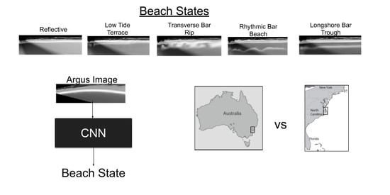
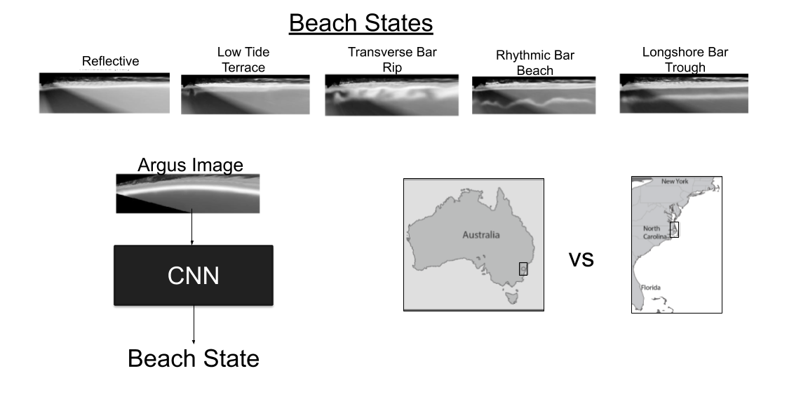
Beach State Recognition Using Argus Imagery and Convolutional Neural Networks

by
Ashley N. Ellenson
1,*,
Joshua A. Simmons
2,
Greg W. Wilson
3,
Tyler J. Hesser
4 and
Kristen D. Splinter
2
1
School of Civil and Construction Engineering, Oregon State University, Corvallis, OR 97330, USA
2
Water Research Laboratory, School of Civil and Environmental Engineering, UNSW Sydney, Sydney, NSW 2093, Australia
3
College of Earth, Ocean and Atmospheric Sciences, Oregon State University, Corvallis, OR 97330, USA
4
United States Army Corps Engineer Research and Development Center, Vicksburg, MS 39180, USA
*
Author to whom correspondence should be addressed.
Remote Sens. 2020, 12(23), 3953; https://doi.org/10.3390/rs12233953
Submission received: 29 October 2020 / Revised: 19 November 2020 / Accepted: 24 November 2020 / Published: 3 December 2020
(This article belongs to the Special Issue Advances in Remote Sensing in Coastal and Hydraulic Engineering)

Abstract

:
Nearshore morphology is a key driver in wave breaking and the resulting nearshore circulation, recreational safety, and nutrient dispersion. Morphology persists within the nearshore in specific shapes that can be classified into equilibrium states. Equilibrium states convey qualitative information about bathymetry and relevant physical processes. While nearshore bathymetry is a challenge to collect, much information about the underlying bathymetry can be gained from remote sensing of the surfzone. This study presents a new method to automatically classify beach state from Argus daytimexposure imagery using a machine learning technique called convolutional neural networks (CNNs). The CNN processed imagery from two locations: Narrabeen, New South Wales, Australia and Duck, North Carolina, USA. Three different CNN models are examined, one trained at Narrabeen, one at Duck, and one trained at both locations. Each model was tested at the location where it was trained in a self-test, and the single-beach models were tested at the location where it was not trained in a transfer-test. For the self-tests, skill (as measured by the F-score) was comparable to expert agreement (CNN F-values at Duck = 0.80 and Narrabeen = 0.59). For the transfer-tests, the CNN model skill was reduced by 24–48%, suggesting the algorithm requires additional local data to improve transferability performance. Transferability tests showed that comparable F-scores (within 10%) to the self-trained cases can be achieved at both locations when at least 25% of the training data is from each site. This suggests that if applied to additional locations, a CNN model trained at one location may be skillful at new sites with limited new imagery data needed. Finally, a CNN visualization technique (Guided-Grad-CAM) confirmed that the CNN determined classifications using image regions (e.g., incised rip channels, terraces) that were consistent with beach state labelling rules.

Graphical Abstract

1. Introduction

The temporal evolution of nearshore morphology is a key area of active research within the coastal community. Nearshore morphology dictates wave breaking patterns and nearshore circulation, which is important in understanding nutrient transport and determining recreational safety and erosion risk [1,2,3]. For example, urban beaches may experience high levels of pollutants entering the surfzone during storms from run-off and pose a health risk to swimmers as well as the local ecosystem. The nearshore morphology affects the generation of bores and nearshore currents that ultimately influence the time and length scales of pollutant mixing, dispersal and advection [4,5]. Similarly, rip currents are the leading cause of death at beaches globally and pose a significant risk to swimmer safety [6]. Bathymetric rip currents are more likely to develop when undulating morphological features are present and are common in the Rhythmic Bar Beach (RBB) and Transverse Bar Rip (TBR) beach states [6,7,8]. Lastly, coastal erosion impacts coastal communities via loss of usable beach amenity and property [9,10]. Nearshore morphology preceding a storm has been shown to influence the levels of shoreline and dune erosion [11,12].
Nearshore morphology can be detected in the surf zone remotely using video cameras. Time-averaged images of the nearshore surf zone, for example from Argus cameras, can be used to detect the shape of sandbars because of the tendency of waves to preferentially break over these higher topographic features [13]. Nearshore morphology is generally considered to exist in consistently-occurring patterns known as beach states [8,14], and the occurrence of these states has been found to correlate with incident wave conditions and sediment grain size [15]. Time series of beach state observations have been used to qualitatively validate modelling studies of sandbar evolution [16,17,18,19,20,21], to gain a general understanding of the behavior of a specific beach system [14,22,23,24,25,26,27], and to determine the level of recreational hazard that exists within the nearshore system [28]. A widely-used beach state classification scheme is that of Wright and Short [8], who defined five distinct sandbar morphology states illustrated in Figure 1. The modal beach state at a given beach depends on the dominant incident wave energy, tidal range, and local sediment size [29,30]. The reflective (Ref) state is the lowest energy state, characterized primarily by waves breaking at the shoreline and an absence of offshore sandbar features. The Low Tide Terrace (LTT) state represents intermediate to low wave energy, with bar welding to the shoreline and the potential for weak rips to be present. The Transverse Bar Rip (TBR) state represents intermediate wave energy with rip circulations. The Rhythmic Bar Beach (RBB) state represents intermediate-high energy, and has a contiguous trough separating the bar from the shoreline, and a bar exhibiting rhythmic crescentic patterns due to offshore-directed rip currents. Lastly, the Longshore Bar Trough (LBT) state represents intermediate to high wave energy, with a contiguous trough; however, rip currents are not as strong as in the RBB state, so the sandbar lacks rhythmicity and extends linearly alongshore.
In Argus time exposure (timex) products, sustained breaking over topographic features (sandbars) appears as bright white bands, and the resulting spatial pattern can be categorized into a beach state [16,24,31,32]. Specific morphological features, such as the position of the sandbar, shoreline or rip locations have been previously derived from Argus timex imagery [18,20,26,33]. While these previous methods are successful in identifying specific morphological features of interest, they require a number of pre-processing steps to extract features (e.g., quasi-linear features such as sandbar crests or shoreline position). Also, the methods are calibrated for specific sites, and may not transfer successfully to other locations [34]. Nearshore optical remote sensing data should be exploited in a scalable and generic way, thereby advancing our understanding of coastal processes at different sites [35,36,37]. Our current mathematical formulations cannot extract meaningful physical information (such as depth limited wave breaking) from remotely sensed imagery. Machine learning techniques may offer a potential path forward, however, because their underlying extremely flexible mathematical formulations can be adapted to detect physically relevant patterns in imagery.
Machine learning techniques have been previously used in a variety of coastal applications [38,39,40]. In contrast with previous studies, the input to the machine learning alogrithm in this study is imagery. Other machine learning/coastal imaging studies have used machine learning as a measurement technique for hydrodynamic quantities such as significant wave height in laboratory settings [41] and in the field [42], and for morphological properties such as grain size [43] and laboratory bed level [44]. Machine learning has also been used for segmenting and classifying coastal images [45], improving shoreline detection [46], classifying wave breaking type [47], and predicting wave run-up [48].
This study uses a convolution neural network (CNN) to automate the classification of beach state from images with limited pre-processing steps. The paper is organized as follows. Section 2 describes the dataset in this study that is derived from two different sites: Narrabeen, New South Wales, Australia; and Duck, North Carolina, United States. Section 3 describes the methods, including the general CNN model and the specific implementation used for the present study. The suitability of a CNN to classify beach state at each location is explored in Section 4, followed by a discussion of the results in Section 5 and conclusions in Section 6.

2. Field Sites and Data

2.1. Field Sites

Figure 2 shows the location of the two study sites. The first site is a sandy barrier beach located at the U.S. Army Engineer Research and Development Center Field Research Facility (FRF) in Duck, North Carolina. The wave climate at Duck is seasonal, with higher incident wave energy in the winter, and lower incident wave energy in the summer [49]. The annual average significant wave height is 1.1 m, with waves tending to come from the south during spring and summer, and from the north during winter. Winter storms consist of both extra-tropical (north-easters) and tropical (hurricanes) cyclones. The mean spring tide range is microtidal at 1.2 m. The beach slope averages 0.108 at the foreshore, and decreases with distance offshore to 0.006 at 8 m depth [50]. The sediment is comprised primarily of medium to fine grain quartz with finer sands further offshore [51]. The median grain size between the bar and the shoreline is approximately 0.5 mm, with 20% carbonate material, while offshore of the bar the median grain size becomes 0.2 mm [49]. This beach generally is classified as an intermediate beach [14] and can frequently have at least one or two sandbars present [52].
The second study site, Narrabeen-Collaroy (herein refered to as Narrabeen) is an embayed beach located in Sydney, Australia (Figure 2, right panel). The average annual wave climate is of moderate to high energy (average significant wave height of 1.6 m) [53]. There is generally a background SSE swell generated by mid-latitude cyclones crossing the Tasman sea, south of Australia. Similar to Duck, Narrabeen sees higher wave energy in winter, and lower wave energy in summer. The summer waves have shorter periods than in winter, and are a combination of both SE swell and local north-easterly sea breeze waves. The winter waves have longer periods, and are generated by storms that consist of mid-latitude cyclones from the south, east-coast lows generated near the NSW coast, and tropical cyclones from the northeast. The mean spring tide range is microtidal at 1.3 m [53]. The sediment is comprised of fine to medium quartz sand with a median grain size of 0.3 mm, and 30% carbonate fragments. Due to the embayed nature of this beach and the predominant SSE swell, there is an alongshore gradient in wave energy and in beach state caused by wave refraction and headland-induced diffraction effects. As a result the more exposed sections of the beach in the north of the embayment are commonly dissipative-intermediate beach states, whereas the more sheltered southern end of the embayment (the location of the present study) is typically classified as reflective-intermediate beach states [54].

2.2. Dataset

The dataset in this study is comprised of orthorectified time exposure (timex) grayscale imagery collected hourly from Argus stations [13], over a period 1987–2014 for Duck, and 2004–2018 for Narrabeen. At Duck the images were combined from one to three different camera views (depending on the year and how many cameras were installed at the time) spanning the area of the beach north of the FRF pier, while at Narrabeen the images were from a single camera view looking north towards the stretch of beach in the center of the embayment (see Figure 2). Effects of poor lighting (due to sun angle or cloud cover), or a lack of wave-breaking signal (due to low waves or a high tide), were reduced by averaging all hourly timex images taken throughout the day into a single daytimex image for each day. The oblique daytimex images were then orthorectified onto a domain of 900 m alongshore by 300 m cross-shore, with a ground resolution of 2.5 × 2.5 m grid (same for both sites). In the case of Duck, multiple camera views were merged following [55]. The orthorectified daytimex images were then bilinearily interpolated to 512 × 512 pixels, following standard machine learning practices where images are reshaped to be square before being input to convolutional neural networks [56].
Figure 1 shows example imagery from Duck and Narrabeen, which highlight several notable differences between the two sites. At Narrabeen, areas outside of the camera field of view are marked in black, resulting in two black triangular spaces in the left side (south side) of the image at this site. At Duck, artifacts of the camera merging result in a diagonal seam separating the images from the three cameras. Additionally, the three cameras at Duck do not always share the same intensity histogram, which can result in non-uniform shading throughout the merged image. Finally, the Narabeen beach exhibits a noticeable curvature in its shape, which is in contrast to the straight coastline at Duck.

3. Methods

Machine learning is based on learning patterns within data by learning correlations between input and a specified output (also called a ‘target’). The branch of machine learning applied in this study is called classification, whereby the targets are discrete classes rather than continuous variables. The Convolutional Neural Network (CNN) technique used here (see Section 3.2 for technique details) is a specific deep learning classification technique that uses supervised learning, meaning the outputs are known a-priori for a set of pre-defined training cases (see Section 3.1 for the explanation of the targets). Once the relationships between input and output are learned from the training data, the CNN is then tested on data from outside the training set to determine its out of sample accuracy. The code for this project can be found in Supplementary Materials.

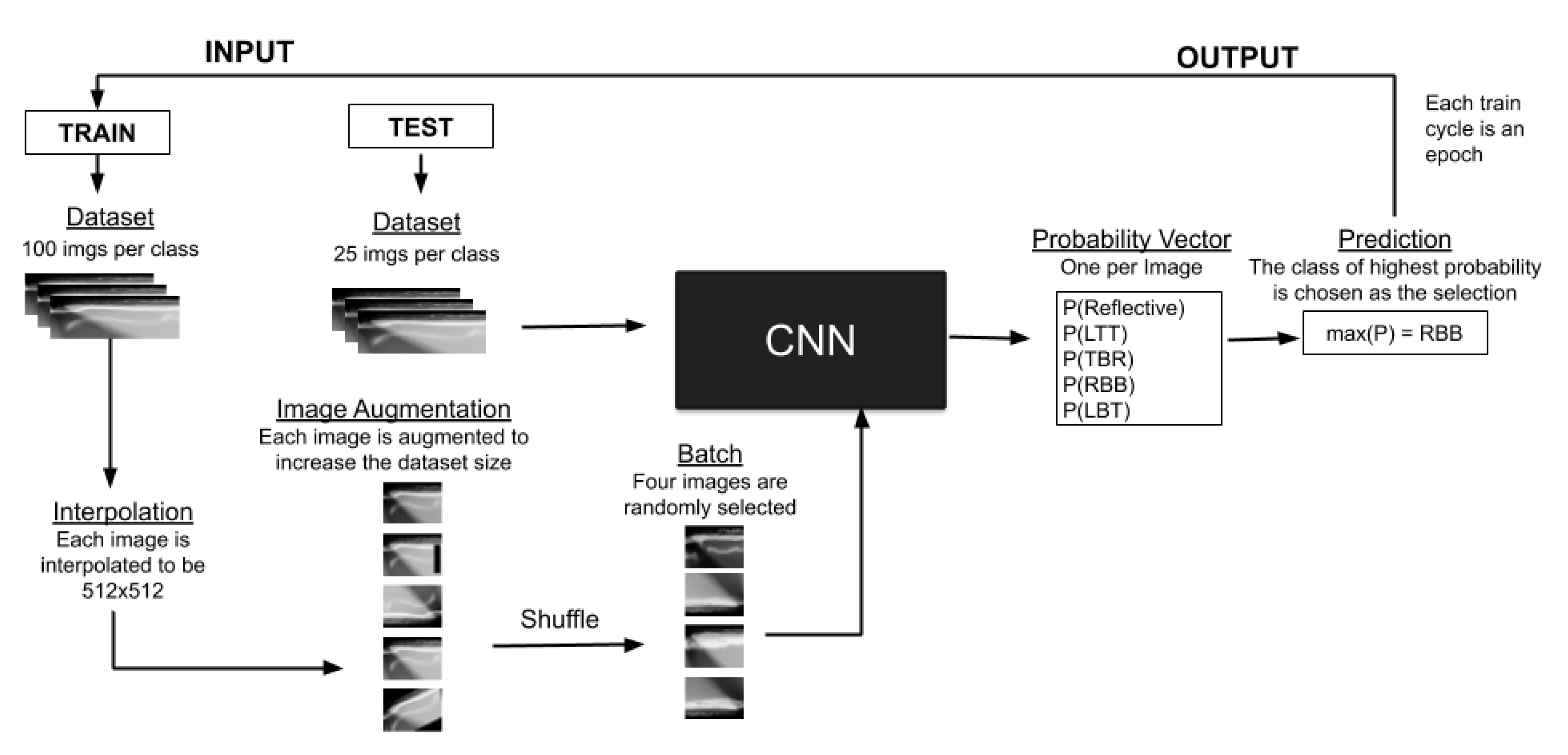
3.1. Dataset Preparation: Manual Labelling and Augmentation

Supervised learning requires a set of manually-classified images used for training and testing. In this study, the target is one of five beach state classes described in Section 1 and the input is an Argus time exposure image. From the 10+ years of daytimex images available from the two sites, 125 images per class (per beach state) per site were selected that were consistent with the description from [8]. Of these, 100 were reserved for training (per class per site, so 1000 total), and 25 for testing (per class per site, so 250 total). The images were labelled by a single person (the first author) in order to minimize labelling inconsistencies that might occur among different labellers. The labelling considered the visible wave breaking patterns, with each image considered independently from the others and in a randomized order. The labeller selected the images wherein only one beach state was visible (no longshore variability of beach states or shape ambiguity, see Section 5.1 for further discussion on beach state labelling challenges). The test dataset was also labelled by the four co-authors independently, for the purposes of benchmarking the CNN model skill in comparison to inter-labeller agreement (see Section 4.1 for further explanation and results).
Deep learning requires large (on the order of thousands of images) amounts of input data for training, and performance can usually be improved by the addition of more training data [57]. In this study, the amount of data was limited by the number of times each state occurred over the time period spanned by the dataset, and the number of images which clearly exhibited only one beach state (see Section 5.1). CNN performance typically benefits from larger dataset sizes than available for this study. As such, image augmentation [58] was used to increase the number of images in the dataset. Five total augmentations were applied, increasing the number of images to 3000 images per site, or 6000 images total. The augmentations included: (1) simultaneous horizontal and vertical flip, (2) random rotation up to 15 degrees, (3) random erasing of 2–8% of the image, (4) random horizontal and vertical translations to a maximum of 15% in the horizontal and 20% in the vertical, and (5) image darkening by gamma correction (power law transform) with a gain of 1 and gamma of 1.5.

3.2. Convolutional Neural Network

This study uses the CNN architecture Resnet-50 [59]; see Appendix A for detailed information about the architecture. The CNN predicts a beach state label (y) based on an input Argus image (x). The algorithm learns this relationship in the form of parameters of a function (f) that maps the input image to the beach state label; y = f ( x ) . Figure A1 shows the details of this function, which has here been represented as an operator, f. In the case of the CNN, the function f comprises two key steps: (1) feature extraction, in which important spatial structures from the input are extracted (e.g., linear or rhythmic features); and (2) class prediction, in which a neural network is used to map the extracted features from step 1 into a predicted beach state based on learned relationships between the spatial features found in step 1 and the associated targets [57]. Historically, when machine learning techniques are applied to imagery, Steps (1) and (2) are performed separately, and so each are separately optimized. In contrast, the deep learning CNN algorithm combines steps (1) and (2) into the same optimization. For each input image, the model outputs a vector of ( k × 1 ) probabilities, where k is equal to the total number of beach states (5). The entry with highest probability is chosen as the CNN label prediction.
During the supervised training, the performance of the model is optimized by minimization of a cross-entropy cost function with respect to the CNN free parameters. Figure 3 shows a schematic of the iterative training procedure. For many CNN studies, a pre-trained CNN is used, meaning that the parameters (the convolutional filter weights) of the CNN have already been optimized to identify objects (e.g., animals, faces, buildings), in a different dataset, such as ImageNet [60]. Pre-trained models were considered in this study, where the final neural network (classification step) was retrained. However, the pre-trained models failed to focus on the bathymetric regions relevant to beach state classification. Therefore, the entire Resnet-50 CNN was trained ‘end-to-end’, meaning that all of the parameters of the entire base model were altered, similar to [42].
During one training epoch, the CNN was fed the entire augmented data set (3000 images) in batches of four randomly-selected images at a time; batch sizes of eight, 12 and 36 images were also tested, but four was found to be the optimal batch size, where training loss was lowest. The training of the CNN is stochastic due to the random seeding of the original parameters, the optimization routine used during training, and the random batches of data selected as input in an epoch. The effects of this randomness on the reported accuracy of each model was assessed by training an ensemble of 10 CNNs for each experiment.

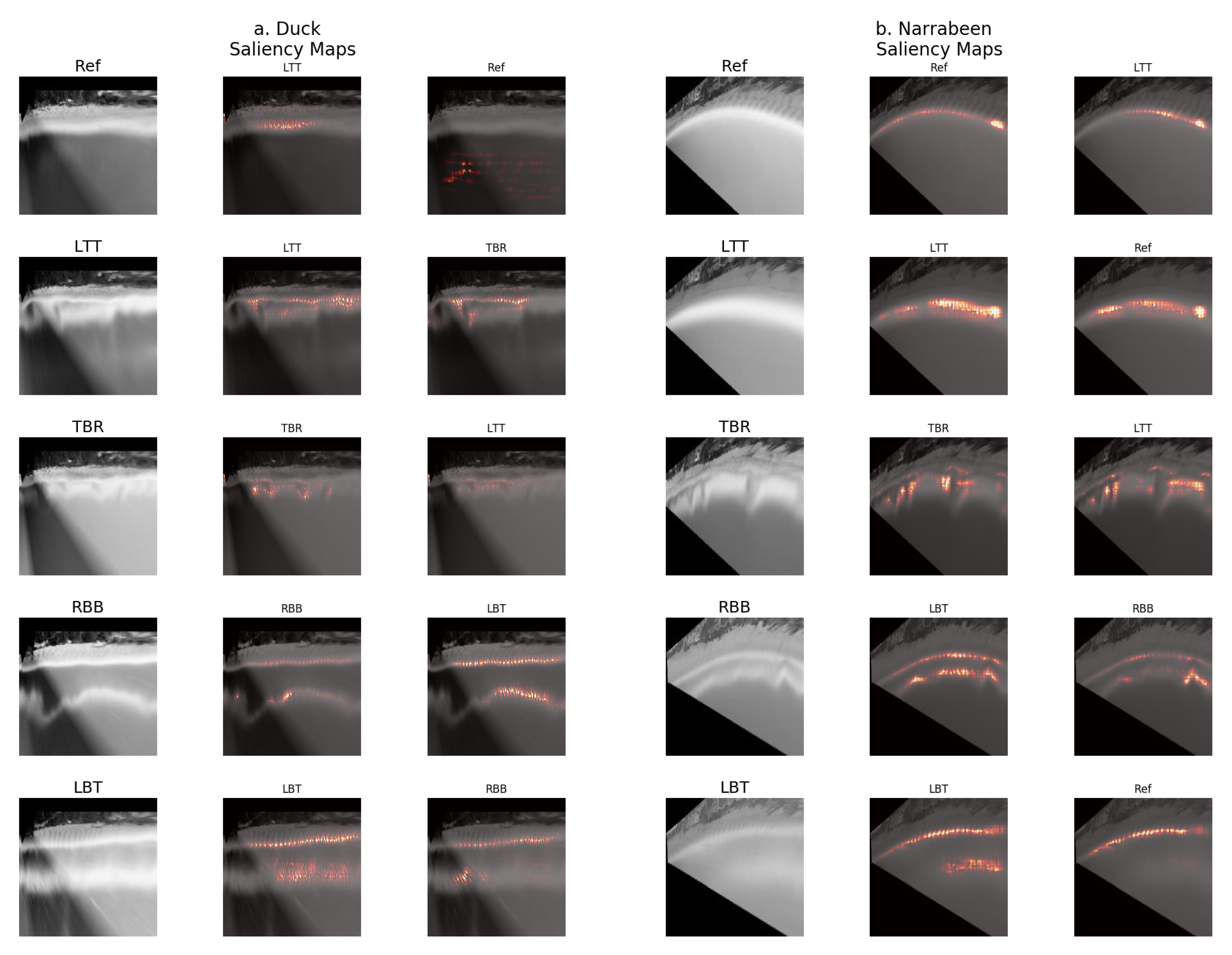
3.3. Visualization: Saliency Maps

Model visualization refers to techniques for inspecting a trained CNN model to determine how its predictions are made. Visualization can be used to confirm that a model’s classifications are based on appropriate qualitative features of beach states, as opposed to other non-relevant features contained in the training data. The model visualization technique used in this study, Guided Grad-CAM, highlights which pixels are most important in the CNN’s final prediction by incorporating information from the two steps of the deep learning process: (1) feature extraction and (2) classification [61]. Guided Grad-CAM is a combination of two visualization techniques that extract information from images: (1) Guided back propagation (GBP) extracts information from the feature extraction step; and (2) class activation maps (CAMs) extract information from the classification step. GBP identifies specific pixels associated with relevant spatial structures [62,63], which in the present study might include linear or curved sandbar shapes or shorelines. The pixels identified by GBP are those that provided the strongest signals to the optimization routine during cost function minimization [62]. On the other hand, CAMs identify the pixels which have the largest contribution to classifying an image as a specific class [64]. Guided Grad-CAMs combine both GBP and CAM techniques by multiplying their outputs together, resulting in visualizations called “saliency maps” that are both spatially detailed and class-specific. Specific to this study, if the CNN has been trained successfully, the pixels highlighted by the Guided Grad-CAM should correspond to the regions showing patterns of wave breaking associated with each beach state class.
Example saliency maps for Duck and Narrabeen for each state are shown in Figure 7 (discussed further in Section 5.1). Visual inspection of the saliency maps showed that approximately 70% had highlighted areas of specific relevance to beach states (e.g., incised rip channels for TBR, swash and off-shore bar for LBT), as in the examples shown.

3.4. Experiments

Three 10-member ensembles of CNNs were trained. The first two ensembles were single-location ensembles, meaning that the training data came from one location (Duck or Narrabeen). The CNN ensemble trained at Duck is hereafter referred to as Duck-CNN, and the CNN ensemble trained at Narrabeen is hereafter referred to as Nbn-CNN. The third ensemble was a combined-location ensemble, meaning that training data came equally from both Narrabeen and Duck, hereafter referred to as combined-CNN. Each CNN was fed 3000 training images (including augmented images), with the combined-CNN using 1500 images from each location, where the images were chosen randomly.
Each single-location ensemble was tested at both locations in self and transfer tests. As the combined-location ensemble was trained with data from both locations, it did not have a transfer test. Overall performance metrics F1, normalized mutual information, and Matthews correlation coefficient were evaluated following [65]. However, the conclusions drawn from the three metrics were similar, so only the F-score is reported herein. The F-score (See Appendix B for a definition) ranges between 0 and 1 with a higher F-score value indicating better performance. Per-state accuracy is also reported to assess state-specific performance of the CNN, and similarly confusion matrices were calculated to determine if biases were present where two or more states were consistently confused with each other. The F-scores and accuracies presented are the average of the 10 CNNs for each ensemble.
Finally, experiments were performed to assess transfer skill as a function of training data composition, and is presented in Section 5.3. Specifically, the goal was to determine the percentage of data required from each site to reach skill comparable to the single-location tests. In these experiments, data was incrementally added from the transfer site as percentages of the total. For example, if the CNN was originally trained at Duck, then data from Narrabeen were added. Eight total experiments were performed, with ratios of Duck to Narabeen training data ranging from 0:100 to 100:0 in 5% increments keeping the total number of training data constant (3000 images). The F-score was assessed at each increment to determine the percentage of data required from each location in order to reach skillful performance.

4. Results

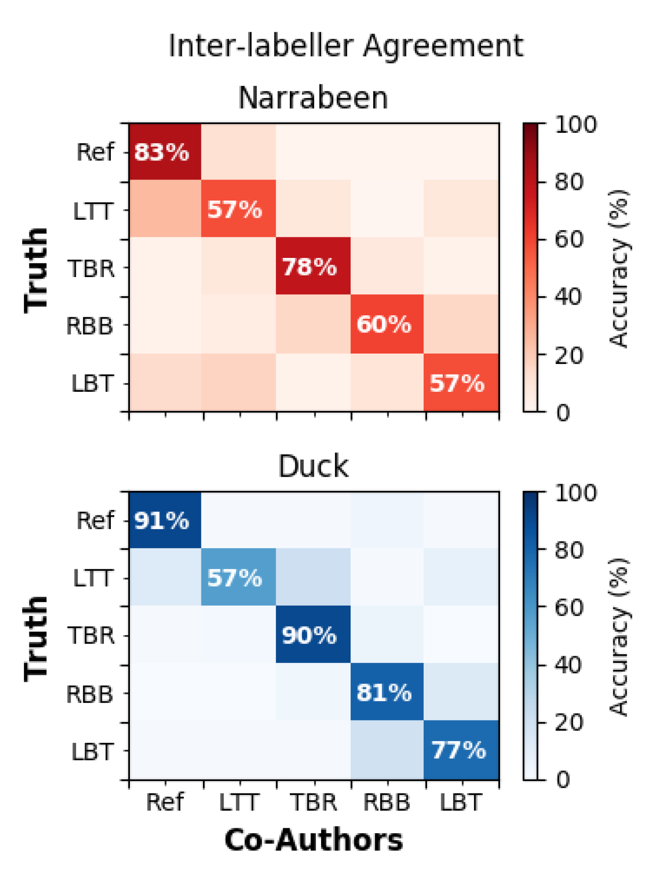
4.1. Inter-Labeller Agreement
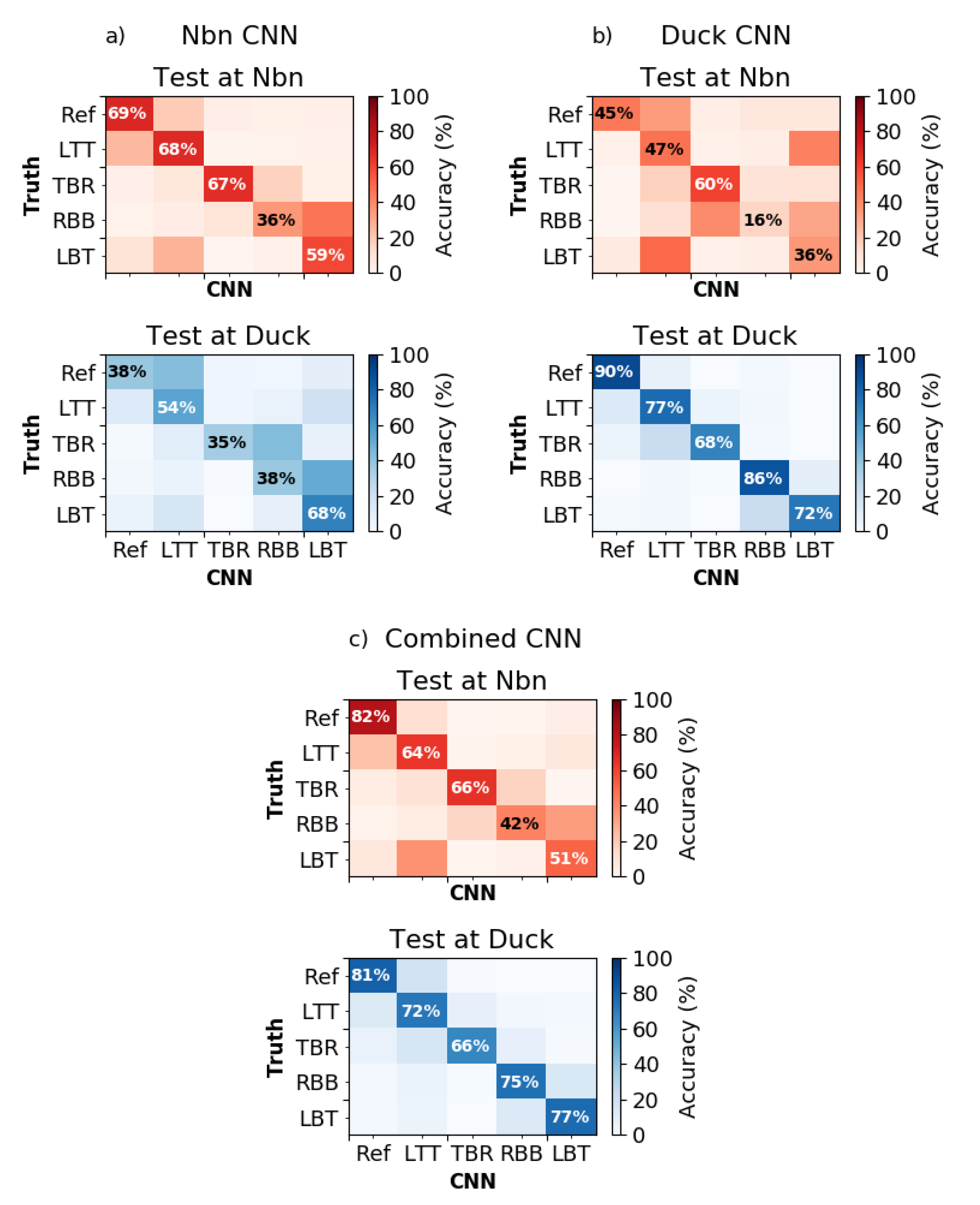
Human performance is commonly used as a benchmark for machine learning skill quantification [66]. In this study, the ”true” label is defined as the label chosen by the primary labeller (the first author). However, it is acknowledged that the same label may not be chosen by another labeller, even among domain experts, owing to the inherently “fuzzy” nature of beach state classification (discussed further in Section 5.1). A human-performance skill benchmark was therefore defined by comparing the true labels to ones chosen by alternative labellers (the co-authors). Figure 4 shows the results of the confusion table and per-state accuracy for the labeller agreement on the validation set.
Specific recurring errors were noted in the inter-labeller comparisons when considering individual beach states. For both locations tested here, the lowest per-state agreement was the LTT state (57%); for Narrabeen, 24% of LTT images were mislabelled as the lower-energy adjacent Reflective state, while for Duck, 21% of LTT images were mislabelled as the adjacent, but higher energy, TBR state. These two cases illustrate the most common reason for misclassification: confusion between adjacent states that belong to a similar energy regime and therefore have similar morphology. Confusion also existed between non-adjacent states, however, that had similar morphological characteristics. For example, at Narrabeen, LBT was confused with either LTT (17% of LBT images) or Reflective (13% of LBT images). LBT and LTT states are similar in that both are linear sandbars, however LBT is found further offshore and is always associated with a trough. LTT is a lower energy sandbar configuration with bar welding to the shoreline, and can have a trough during high tide when the terrace is flooded. The confusion at Narrabeen may be due to the relatively narrow surfzone width, and so the distance between the shoreline and the sandbar was small in many images. This confusion was also reported in another study [16] at nearby Palm Beach, NSW, a site that displays similar nearshore morphology to Narrabeen.

4.2. CNN Skill

Figure 5 summarizes the F-scores obtained by the CNN. In general, the skill was highest when the training and testing data were from the same location, in which case, CNN F-scores were comparable to inter-labeller agreement as reported in Section 4.1. Duck-CNN F-score was 0.80 compared with 0.79 for manual agreement, and Nbn-CNN F-score was 0.59 compared with 0.57 for manual agreement. The CNN trained on the combined training dataset (combined-CNN) predicted beach state more accurately on the combined test dataset (test data from both locations, black boxes Figure 5) than either of the single-site CNNs. Specifically on the combined dataset, the combined-CNN reached an F-score of 0.68, compared with Duck-CNN F-score of 0.61 and Nbn-CNN F-score of 0.53. Interestingly, the combined-CNN also slightly outperformed the Nbn-CNN at Narrabeen (F-Score = 0.61), although the two were equally skillful to within the variability of their respective CNN ensembles.
The transfer skill of the CNN, defined as the skill when trained at one location and then tested at another location, varied depending on the training data set. The Nbn-CNN skill was reduced by 24% when transferred to Duck, which was less than the 48% reduction in skill for the Duck-CNN when transferred to Narrabeen. This suggests that the correlations between sandbar characteristics and beach state learned at Narrabeen were more informative when predicting beach state at Duck than vice versa. It is speculated this could be due to the relatively smaller length scales at Narrabeen, and therefore the requirement that the CNN learn relatively finer sandbar features at Narrabeen compared to Duck. That is, the finer features learned by Nbn-CNN may have remained applicable when predicting beach states at Duck, while larger features learned by Duck-CNN were less applicable when predicting beach states at Narrabeen. See Section 5.2 for further discussion and quantification of length scales at the two sites.
Figure 6 shows the confusion tables from each of the six tests. Overall, for all self-tests, the CNN outperformed random choice (accuracy > 20%) and the accuracy was comparable to inter-labeller agreement (Figure 4). The self tests (i.e., trained and tested at the same locations) resulted in slightly higher per-state accuracy at Duck (68–90%) than at Narrabeen (36–69%). For both sites, the highest accuracy was in the classification of the low-energy Ref state, while the lowest accuracy of the CNN was in classifying the rhythmic states of RBB (Nbn) and TBR (Duck). The Nbn-CNN confused the RBB state most often with LBT, with 47% of the RBB images misclassified as LBT. Note that the RBB and LBT states both correspond to an offshore sand bar with a distinct trough, with the differentiating factor being the degree of bar curvature. Also at Narrabeen, 27% of LBT images were confused for LTT, an error that also occurred in the manual classification experiment (17% of LBT images confused for LTT). The Duck-CNN confused the TBR state most often with LTT, with 28% of the TBR images classified as LTT. The TBR and LTT states both correspond with bar welding, and both may include rip currents, with the differentiating factor being a larger number and size of rip currents present in TBR.
For the transfer tests, the per-state accuracy decreased for the majority of states compared to the self tests. Per-state accuracy ranged between 35–68% (Nbn-CNN at Duck) and 16–60% (Duck-CNN at Nbn). Similar to the overall skill trends (see Figure 5), Nbn-CNN transferred better than the Duck-CNN when assessed with per-state accuracy. The per-state transfer accuracy for Nbn-CNN was highest for LBT (68%), and lowest for the Ref, TBR and RBB states (accuracies of 38%, 35% and 38%, respectively) when tested at Duck. The confusion for these states was primarily adjacent and up-state (Ref confused as LTT, TBR confused as RBB, and RBB confused as LBT). Additionally, the LTT images were confused as LBT 48% of the time. For the Duck-CNN transfer test, the bar states characterized by rhythmic features (TBR and RBB) were mainly labelled as TBR (44% percent of RBB images were classified as TBR), and the linear states (Ref, LTT, LBT) were labelled as LTT. Overall, the Nbn-CNN had higher per-state accuracy at Duck than the Duck-CNN had at Narrabeen. The main confusion for Nbn-CNN at Duck was up-state, adjacent-state confusion, whereas the Duck-CNN at Nbn had an LTT bias. Possible explanations for state confusions are detailed in Section 5.2.
The combined-CNN that was trained equally with data from Narrabeen and Duck showed overall good skill and per-state accuracy at both beaches (42–82% at Nbn and 66–81% at Duck). Compared to the Nbn-CNN at Narrabeen, it exhibited less confusion for the Ref class, and similar confusion for RBB (34% for combined-CNN versus 47% for Nbn-CNN of RBB images were confused for LBT) and LBT (38% for combined-CNN versus 27% for Nbn-CNN of LBT images were confused for LTT). Compared to the Duck-CNN at Duck, it exhibited similar confusion for TBR (16% for combined-CNN versus 28% for Duck-CNN of images were confused for LTT). The combined-CNN also resulted in slightly lower per-state accuracy for Ref, LTT and RBB states (accuracy reductions of 9%, 5%, and 11% for each state, respectively) at Duck.

5. Discussion

5.1. Beach State Classification

It is notable that many of the misclassifications made by the CNN (Figure 6) and the disagreement between labellers (Figure 4) can mostly be attributed to states that are adjacent to one another in the ordered list defined by Wright & Short [8]. This implies that, as expected, adjacent states have similar morphology and may be easily mistaken for one another. The use of the classification system of Wright and Short [8] in this study implicitly assumes that instantaneous beach morphologies, as observed by Argus imagery, can be categorized into discrete states. This is an approximation, however, as sandbars exhibit a continuum of shapes as they evolve between configurations [15,24,26], and may never reach a true equilibrium state. This is especially true during the slower, down-state evolution of sandbar configuration (i.e., RBB to TBR to LTT) as described by [14]. During the labelling process, the most dominant state was used as the classification, but in practice ‘pure’ beach states are not present in all images. Therefore, achieving 100% accuracy for an ambiguous beach state is impossible. Three predominant issues were identified by the authors as challenges in determining beach state: (1) labeller perception, (2) alongshore variability of bar state and (3) sandbar state ambiguity due to the nearshore evolving between states.
Since there are no rigorous, quantifiable rules which delineate each beach state, a state identification for a specific image could vary due to labeller perception. Differences in labeller perception can occur either because the labeller is different (a different person), or the labeller might have a different perception on a different day. While the labels used to train and test the CNN in this study were made solely by the first author to limit labeller perception bias within the model training, the co-author labelling experiments (see Figure 4) highlight the challenges with labeller perception and the overall complexity in classifying unique beach states. Specifically, the co-authors did not achieve 100% agreement on any one state. Most notably, there was more confusion among the different labellers for Narrabeen than Duck, suggesting this beach may exhibit more complex or ambiguous beach states (discussed further in Section 5.2).
Alongshore gradients and irregularities in hydrodynamic forcing might impose alongshore variability of sediment transport and resultant sandbar patterns in one image. Therefore, one image might clearly exhibit more than one beach state in the alongshore (for examples, see Figure 7). For the two test sites presented here, the pier at Duck can affect sediment transport at a distance of up to 500 m [67] and at Narrabeen strong alongshore gradient of breaking wave height due to wave sheltering from the adjacent headland results in alongshore variability in the dominant beach states [54]. Additionally, as the morphology evolves between states, the sandbar shape can exhibit characteristics of adjacent classes in one image and therefore have an ambiguous classification. In either of these cases (i.e., alongshore variability or shape ambiguity), a more accurate classification would be a mixture of classes. However, since the CNN in this study is a single-label classification tool, only a single discrete target class can be given for training, potentially causing model and labeller disagreement.
Saliency maps can be used to troubleshoot model/labeller disagreement (see Section 3.3 for a discussion on saliency maps). The representative saliency maps in Figure 7 illuminate which regions of the image were chosen by the CNN to be important for classification. Specifically, they show that the CNN can differentiate between states due to physical characteristics such as sandbar welding or rhythmicity. For images labelled as Ref, salient (warm color) areas are focused on the breakers at the shoreline or dark areas just offshore that indicate a conspicuous absence of breaking. Salient areas for images labelled as LTT are also focused on shorebreak, which can be associated with few rips and bar welding that characterize the LTT state. The curved wave breaking patterns connected to the shoreline that can be associated with rip currents and intermittent welded sandbars which characterize the TBR state are the salient areas for the TBR state. For images labelled RBB salient areas are focused on rhythmic features. Salient areas are focused on an offshore bar and the shoreline, which indicates the existence of a trough for images labelled LBT.
Despite the CNN being a discrete classification tool, the saliency maps suggest it can also detect the presence of multiple beach states within one image, and/or beach state ambiguity. For example, the LTT image at Duck (Figure 7a, second row) could plausibly be labelled as either LTT or TBR, depending on which side of the image the labeller focuses. Incised rip channels, characteristic of the TBR state, exist in the left side of the image, while a terrace, characteristic of the LTT state, exists on the right side of the image. The resulting first and second choice saliency maps for this image highlight the LTT and TBR features, respectively. Both of these choices have validity, but as currently implemented the CNN only reports the first choice as its output. The use of saliency maps to develop a multi-output classification or a non-discrete labelling system [26] are possible improvements to the present model. For example, object localization, a deep learning technique developed by [68], is a technique wherein the CNN identifies the location of objects within a picture using class activation maps. Object localization could potentially be adapted as a way to identify and quantify alongshore variable bar states.

5.2. Site Imagery Differences Affecting State Identification

The lower skill at beach state identification at Narrabeen by both the CNN and by the co-authors suggests that classifying beach state at Narrabeen is a more ambiguous problem than at Duck. Similarly, the probabilistic output of the CNN (the step before the final maximum-likelihood selection step) showed that the average probability assigned to its classification was 85% and 76% at Duck and Narrabeen, respectively. The different choice probabilities imply that the CNN had slightly less confidence in its predictions at Narrabeen, which is consistent with the relatively lower skill that was obtained. The ambiguity of beach state at Narrabeen was possibly due to two reasons: (1) difficulty in consistently identifying the shoreline; and (2) smaller length scales at Narrabeen.
As shown in the saliency maps (Figure 7), the CNN typically identifies the shoreline and offshore features when classifying the states. However, the optical signature of the shoreline at these sites can be quite different. The shoreline at Narrabeen can be identified in time exposure imagery in two ways: by the higher image intensities associated with swash motions or, more frequently, by lower intensities associated with wet, dark sand. In contrast, the shoreline at Duck is consistently identifiable by higher image intensities due to swash motions [67,69,70]. The lack of consistency of shoreline intensity at Narrabeen results in greater difficulty in identifying the shoreline, thus making beach state labelling more difficult. Specifically, the key difference between LTT/Ref classes and LBT is the distance between the shoreline and the sandbar. At Narrabeen, however, the separation between shoreline and sandbar is less obvious than at Duck, due to the former’s lack of a consistent optical signature of the shoreline.
As described in Section 2.1, the modal bar states at Narrabeen and Duck differ, with Duck existing in a slightly higher (intermediate) energy state more consistently than Narrabeen (intermediate-reflective). Narabeen generally has a morphology that is contained closer to the shoreline, consistent with it being a generally more reflective beach than Duck due to a larger grain size and lower-energy wave climate. A variogram analysis [71,72,73] was performed in the cross-shore and the mean length scales were quantified as the average range of the variograms for the test dataset. The mean length scales of sandbar features at Narrabeen were smaller than at Duck by 5%, 22%, 24%, 13%, and 16% for states Ref, LTT, TBR, RBB and LBT, respectively. This suggests that the cross-shore position of the sandbar is generally further offshore at Duck than at Narrabeen, and so the physical sandbar features, such as rhythmicity or welding, can be more exaggerated at Duck than at Narrabeen. Furthermore, individual beach states at Narrabeen have length scales (as defined by the average range of the variograms) that are more similar to one another (range between 607–627 m), compared to at Duck (range between 664–805 m). Overall, the differences in inter-state length scale variability and overall length scales magnitudes could contribute to the relative clarity of beach state at Duck compared with Narrabeen, leading to higher CNN performance and inter-labeller agreement.

5.3. Data Requirements for Skillful Transfer of the CNN to New Sites

Section 4 presents results from experiments where the composition of training data from each beach was even or completely from one beach. A third set of experiments were performed wherein the percentage of data from each beach in the training set differed. The intention of the experiments was to determine how much data from a different (or new) location was necessary to obtain adequate test skill. This is important when considering the use of such a CNN on new sites where limited training data may be available. Figure 8 shows the F-scores for different ratios of data added to the training set and then tested on each of the three single-location test data sets (Nbn, Duck, Combined).
For the training set ratios which consisted of at least 5% of data from either location, when the CNN was tested on the combined data set the F-score remained within 15% of the max skill (F-score = 0.69) suggesting the model was relatively insensitive to training data composition when presented with a range of diverse images from both sites. In contrast, when the CNN was tested on the individual sites (Duck or Nbn) F-scores decreased if the percentage of images from one location dropped under a certain threshold. At Duck and Narrabeen (blue line in Figure 8), skill became lower than 10% of its maximum value (maximum values of ∼0.8 and ∼0.64 at Narrabeen, respectively) if fewer than 25% of than training data was from Duck. Overall, this suggests for reasonable transferability of the model, a minimum of 25% of the data should come from any new sites proposed.

6. Conclusions

This study applied a convolutional neural network (CNN) to recognize beach states from daytime exposure (daytimex) Argus imagery at two contrasting beaches, Duck, NC, USA and Narrabeen, NSW, Australia. Three CNNs were considered: two trained with data from each of the sites individually, and one trained with data from both sites. The trained models were then tested on images from each site that were not included in the training data. The model results were compared with each other and to the agreement between four domain experts who manually labelled the dataset. The results showed that CNN ensembles that were trained and tested at the same site had skill that was comparable to inter-labeller agreement of the same test data set, and that the overall skill was higher at Duck (F-score = 0.80) than at Narrabeen (F-score = 0.61). CNN per-state accuracy was comparable to inter-labeller per-state agreement for Duck and slightly lower for Narrabeen. For both sites, the highest accuracy was in the classification of the low-energy Ref and LTT states, while the lowest skill of the CNN was in classifying the rhythmic states of RBB (Nbn) and TBR (Duck). The combined-CNN had the highest skill on the combined test dataset (F-score = 0.68, versus F-score = 0.59 and 0.53 for Duck-CNN and Nbn-CNN, respectively). Compared with the self-trained CNNs, it similarly confused RBB with LBT at Narrabeen, and TBR with LTT at Duck, with slightly lower per-state accuracy for Ref, LTT and RBB states at Duck.
When the single-site trained CNN was transferred to the other site, the F-scores dropped by 20% (Nbn-CNN tested at Duck), and 58% (Duck-CNN tested at Narrabeen). In additional transferability tests, the composition of the training dataset was altered to contain different proportions of training images from each of the two locations. Overall, comparable skill (10% of the maximum skill) to the self-trained CNN tests was achieved when at least 25% of the data came from the transfer site. Further, Saliency maps were used to identify the specific image regions that were used for CNN decision making. They showed that relevant regions were highlighted for determining beach state classification (e.g., the swash region for the Reflective state, or the offshore bar and shoreline for Longshore Bar Trough), suggesting that the CNN had accurately identified key features that distinguish beach states at these two contrasting sites.
Additionally, the alongshore variability of beach state should be considered in beach state detection in order to extract the most information available from the image. Ultimately, a globally applicable CNN that would be able to detect beach state for all locations could be developed by using labelled data from sites around the world.

Supplementary Materials

Code for this project is available online at https://github.com/anellenson/DeepBeachState. The data is available upon request.

Author Contributions

Conceptualization, A.N.E., G.W.W.; methodology, A.N.E.; software, A.N.E.; formal analysis, A.N.E.; data curation, A.N.E., J.A.S.; writing—original draft preparation, A.N.E.; writing—review and editing, J.A.S., G.W.W., T.J.H., K.D.S.; supervision, J.A.S., G.W.W., T.J.H., K.D.S.; funding acquisition, T.J.H., K.D.S. All authors have read and agreed to the published version of the manuscript.

Funding

Funding for the routine monitoring and Argus camera system at Narrabeen is generously provided by Northern Beaches Council (formerly Warringah Council), the NSW Adaptation Research Hub—Coastal Processes Node (Office of Environment and Heritage), and the Australian Research Council (LP0455157, LP100200348, DP150101339, LP170100161). The work presented by the authors was supported by the US Army Engineer Research and Development Center (ERDC) under PE 6.3 0603734A, Military Engineering Advanced Polymer Development and Littoral Research. KDS and JS are also supported by the NSW Environmental Trust (RD2015/128).

Acknowledgments

The authors would like to thank David Reinert for his preparation of the study site maps. The authors would also like to acknowledge Tom Lippmann for providing validation data from a previous study. The authors wish to thank Prof. Rob Holman (OSU) for the initiation and upkeep of the long-standing Duck Argus Coastal Imaging station with funding from Office of Naval Research, the US Army Corps of Engineers, and the United States Geological Survey.

Conflicts of Interest

The authors declare no conflict of interest.

Appendix A. Convolutional Neural Network Theory

This study uses a pre-defined CNN called Resnet-50 [59], shown schematically in Figure A1. The CNN begins with a feature extraction step, consisting of a convolutional layer followed by convolutional blocks. The convolutional layer includes kernel of weights (treated as free parameters) that are convolved over the image intensity values, resulting in a representation of the image into a new feature space called a feature map. For example, a kernel might act to find edges within the image, resulting in a feature map that contains only the edges of high contrast from the original image. The first convolutional layer in Resnet-50 has 64 kernels that span 7 × 7 pixels, and are applied sequentially to the image with a stride (or lag) of two pixels. The output from the convolutional layer is then fed into a batch normalization layer. The batch normalization step acts to redistribute the values of the feature maps to a Gaussian distribution, which aids in optimization [74]. Next, an activation function (here a R e L U function, R e L U ( x ) = m a x { 0 , x } ) is applied to the batch-normalized values to filter only the positive values output from the convolution step. This allows for the convolutional neural network to calculate non-linear relationships between the input and output. The R e L U output is then fed into an max pooling layer, which reduces the dimensions of the feature map by providing summary statistics of the salient portions of the feature maps. Specifically, the max pooling layer consists of convolving a filter over the image. The filter outputs the maximum value of a feature map within a neighborhood of 3 × 3 pixels and with a stride of two pixels.
Figure A1. ResNet architecture (adapted from Table 1 and Figure 3 of [59]). The modules with learnable parameters are boldface.
Remotesensing 12 03953 g0a1
The output of the first convolutional layer is then passed to a series of “bottleneck” convolutional blocks, Figure A1. As the information passes through the CNN, the original 3 × 512 × 512 block of data (the image) increases in the first dimension due to the number of kernels used, and decreases in the two spatial dimensions due to the use of the 3 × 3 kernels with a stride of two in the convolutional steps. In addition to the sequential connections between each block, the blocks are also connected via skip, or “residual” connections (hence the name ResNet). These residual connections occur through an identity mapping ( y = F ( x ) + x ) , 0 ); meaning that the information from an earlier block ( x ) is directly passed to a later block, skipping the transformations made within the blocks along the way ( F ( x ) ). The residual connections help the algorithm to reduce training error quicker, since they enable information to flow more efficiently and directly through the network to allow better adjustment of the kernel weights in the first layers. The output from the final convolutional block is fed to a global average pooling layer. Similar to the max pooling layer, it serves to reduce the dimensions of the feature maps by providing summary statistics about the feature maps. It outputs the average of each feature map, resulting in a ( k × 1 × 1 ) vector, where k is the number of feature maps (2048 in ResNet50).
After the feature extraction step comes the classification step. This is performed with a traditional machine learning (i.e., not deep learning) technique: a neural network. The output of the global average pooling layer, the flattened vector, is fed into a fully connected neural network that has one layer of neurons. The output of the neural network is in turn passed to a softmax function ( s o f t m a x = e x p ( z c ) c ( z c ) ), which outputs a probability mass vector corresponding to the predicted probability for each class, y ^ . The entry with the highest probability is taken as the class prediction.
Maximum likelihood estimation of the CNN parameters is performed during training by minimization of a cost function calculated over the training data set. For one training example (image, n) with a total of five classes, the cost function is the cross entropy function:
J n ( Θ ) = c = 1 5 y c l o g ( y ^ c )
In this function, the CNN prediction (defined as the entry with the maximum value of the softmax output) is y ^ c , and the true value is y c . The softmax output can be thought of as a modelled probability distribution, where the model is defined by the free parameters of the CNN. The target can be thought of as a Dirac delta function with a ‘1’ entered in the position of the true class. Maximum likelihood estimation is used to determine the free parameters of the CNN that are most likely to predict the true distribution [57]. The maximum likelihood estimation is made by minimizing the cost function with an iterative scheme called stochastic gradient descent (SGD) with momentum. At each iteration step of SGD, the parameters are adjusted according to the value of the gradient of the cost function with respect to those parameters. In this study, mini-batch gradient descent is used, so the parameters are updated with a gradient value that is averaged from four training examples: 1 4 n = 1 4 Θ J n ( Θ ) . Momentum is used to achieve minimization more efficiently, by adding a weighted estimate of the gradient from the previous batch to the adjustment. The specific SGD parameters used in this study were a learning rate of 0.01, and a momentum weight of 0.9. The learning rate was reduced by a factor of 10 if the training loss did not improve (decrease) after 8 epochs. The training was run for 120 epochs, and generally converged after approximately 40 epochs.

Appendix B. Skill Metrics

For a multi-class classification problem, a confusion matrix provides information about which classes were categorized correctly and incorrectly. A confusion matrix Z , is a K × K matrix where K is the number of classes considered in the multi-class problem. The entry in the confusion table z i j represents how many images of class i were classified as class j . The total number of images belonging to a certain class i is defined as x i = i z i j , while the total number of images classified (by the CNN) as a certain class i is defined as y i = j z j i . The specificity, or precision (P), is defined as the number of images that were labelled correctly divided by the number of images labelled as that category:
P = z i i y i
The per-class accuracy, or recall (R), is defined as the number of images that were labelled correctly divided by the total number of images with that label in the dataset:
R = z i i x i
The F-score is defined as the harmonic mean between precision and recall:
F = 2 P R P + R
See References [65,75] for further information on accuracy measures for multi-class classification problems.

References

  1. Holman, R.A.; Symonds, G.; Thornton, E.B.; Ranasinghe, R. Rip spacing and persistence on an embayed beach. J. Geophys. Res. Ocean. 2006, 111. [Google Scholar] [CrossRef] [Green Version]
  2. Turner, I.L.; Whyte, D.; Ruessink, B.G.; Ranasinghe, R. Observations of rip spacing, persistence and mobility at a long, straight coastline. Mar. Geol. 2007, 236, 209–221. [Google Scholar] [CrossRef]
  3. Wilson, G.W.; Özkan-Haller, H.T.; Holman, R.A. Data assimilation and bathymetric inversion in a two-dimensional horizontal surf zone model. J. Geophys. Res. Ocean. 2010, 115. [Google Scholar] [CrossRef]
  4. Inman, D.L.; Brush, B.M. The coastal challenge. Science 1973, 181, 20–32. [Google Scholar] [CrossRef] [PubMed]
  5. Grant, S.B.; Kim, J.H.; Jones, B.H.; Jenkins, S.A.; Wasyl, J.; Cudaback, C. Surf zone entrainment, along-shore transport, and human health implications of pollution from tidal outlets. J. Geophys. Res. Ocean. 2005, 110. [Google Scholar] [CrossRef]
  6. Austin, M.J.; Scott, T.M.; Russell, P.E.; Masselink, G. Rip Current Prediction: Development, Validation, and Evaluation of an Operational Tool. J. Coast. Res. 2013, 29, 283–300. [Google Scholar] [CrossRef] [Green Version]
  7. Castelle, B.; Scott, T.; Brander, R.W.; McCarroll, R.J. Rip current types, circulation and hazard. Earth-Sci. Rev. 2016, 163, 1–21. [Google Scholar] [CrossRef]
  8. Wright, L.D.; Short, A.D. Morphodynamic variability of surf zones and beaches: A synthesis. Mar. Geol. 1984, 56, 93–118. [Google Scholar] [CrossRef]
  9. Leatherman, S.P. Coastal erosion and the United States national flood insurance program. Ocean Coast. Manag. 2018, 156, 35–42. [Google Scholar] [CrossRef]
  10. Helderop, E.; Grubesic, T.H. Social, geomorphic, and climatic factors driving US coastal city vulnerability to storm surge flooding. Ocean Coast. Manag. 2019, 181, 104902. [Google Scholar] [CrossRef]
  11. Thornton, E.B.; MacMahan, J.; Sallenger, A.H. Rip currents, mega-cusps, and eroding dunes. Mar. Geol. 2007, 240, 151–167. [Google Scholar] [CrossRef]
  12. Castelle, B.; Marieu, V.; Bujan, S.; Splinter, K.D.; Robinet, A.; Sénéchal, N.; Ferreira, S. Impact of the winter 2013–2014 series of severe Western Europe storms on a double-barred sandy coast: Beach and dune erosion and megacusp embayments. Geomorphology 2015, 238, 135–148. [Google Scholar] [CrossRef]
  13. Holman, R.A.; Stanley, J. The history and technical capabilities of Argus. Coast. Eng. 2007, 54, 477–491. [Google Scholar] [CrossRef]
  14. Lippmann, T.C.; Holman, R.A. The spatial and temporal variability of sand bar morphology. J. Geophys. Res. Ocean. 1990, 95, 11575–11590. [Google Scholar] [CrossRef]
  15. Wright, L.; Short, A.; Green, M. Short-term changes in the morphodynamic states of beaches and surf zones: An empirical predictive model. Mar. Geol. 1985, 62, 339–364. [Google Scholar] [CrossRef]
  16. Ranasinghe, R.; Symonds, G.; Black, K.; Holman, R. Morphodynamics of intermediate beaches: A video imaging and numerical modelling study. Coast. Eng. 2004, 51, 629–655. [Google Scholar] [CrossRef]
  17. Strauss, D.; Tomlinson, R.; Hughes, L. Numerical modelling and video analysis of intermediate beach state transitions. In Proceedings of the 7th International Conference on Hydroscience and Engineering, Philadelphia, PA, USA, 10–13 September 2006. [Google Scholar]
  18. Plant, N.G.; Holland, K.T.; Holman, R.A. A dynamical attractor governs beach response to storms. Geophys. Res. Lett. 2006, 33. [Google Scholar] [CrossRef] [Green Version]
  19. Siegle, E.; Huntley, D.A.; Davidson, M.A. Coupling video imaging and numerical modelling for the study of inlet morphodynamics. Mar. Geol. 2007, 236, 143–163. [Google Scholar] [CrossRef]
  20. Splinter, K.D.; Holman, R.A.; Plant, N.G. A behavior-oriented dynamic model for sandbar migration and 2DH evolution. J. Geophys. Res. Ocean. 2011, 116. [Google Scholar] [CrossRef] [Green Version]
  21. Dubarbier, B.; Castelle, B.; Ruessink, G.; Marieu, V. Mechanisms controlling the complete accretionary beach state sequence. Geophys. Res. Lett. 2017, 44, 5645–5654. [Google Scholar] [CrossRef]
  22. van Enckevort, I.M.J.; Ruessink, B.G. Video observations of nearshore bar behaviour. Part 2: Alongshore non-uniform variability. Cont. Shelf Res. 2003, 23, 513–532. [Google Scholar] [CrossRef]
  23. Castelle, B.; Bonneton, P.; Dupuis, H.; Sénéchal, N. Double bar beach dynamics on the high-energy meso-macrotidal French Aquitanian Coast: A review. Mar. Geol. 2007, 245, 141–159. [Google Scholar] [CrossRef]
  24. Price, T.; Ruessink, B. State dynamics of a double sandbar system. Cont. Shelf Res. 2011, 31, 659–674. [Google Scholar] [CrossRef]
  25. Ojeda, E.; Guillén, J.; Ribas, F. Dynamics of single-barred embayed beaches. Mar. Geol. 2011, 280, 76–90. [Google Scholar] [CrossRef] [Green Version]
  26. Armaroli, C.; Ciavola, P. Dynamics of a nearshore bar system in the northern Adriatic: A video-based morphological classification. Geomorphology 2011, 126, 201–216. [Google Scholar] [CrossRef]
  27. De Santiago, I.; Morichon, D.; Abadie, S.; Castelle, B.; Liria, P.; Epelde, I. Video monitoring nearshore sandbar morphodynamics on a partially engineered embayed beach. J. Coast. Res. 2013, 65, 458–463. [Google Scholar] [CrossRef]
  28. Short, A.; Hogan, C. Rip currents and beach hazards: Their impact on public safety and implications for coastal management. J. Coast. Res. 1994, 12, 197–209. [Google Scholar]
  29. Masselink, G.; Short, A.D. The Effect of Tide Range on Beach Morphodynamics and Morphology: A Conceptual Beach Model. J. Coast. Res. 1993, 9, 785–800. [Google Scholar]
  30. Loureiro, C.; Ferreira, S.; Cooper, J.A.G. Applicability of parametric beach morphodynamic state classification on embayed beaches. Mar. Geol. 2013, 346, 153–164. [Google Scholar] [CrossRef]
  31. Lippmann, T.C.; Holman, R.A. Quantification of sand bar morphology: A video technique based on wave dissipation. J. Geophys. Res. Ocean. 1989, 94, 995–1011. [Google Scholar] [CrossRef]
  32. Browne, M.; Strauss, D.; Tomlinson, R.; Blumenstein, M. Objective Beach-State Classification From Optical Sensing of Cross-Shore Dissipation Profiles. IEEE Trans. Geosci. Remote Sens. 2006, 44, 3418–3426. [Google Scholar] [CrossRef]
  33. van Enckevort, I.M.J.; Ruessink, B.G. Effect of hydrodynamics and bathymetry on video estimates of nearshore sandbar position. J. Geophys. Res. Ocean. 2001, 106, 16969–16979. [Google Scholar] [CrossRef] [Green Version]
  34. Contardo, S.; Symonds, G. Sandbar straightening under wind-sea and swell forcing. Mar. Geol. 2015, 368, 25–41. [Google Scholar] [CrossRef]
  35. Splinter, K.D.; Harley, M.D.; Turner, I.L. Remote sensing is changing our view of the coast: Insights from 40 years of monitoring at Narrabeen-Collaroy, Australia. Remote Sens. 2018, 10, 1744. [Google Scholar] [CrossRef] [Green Version]
  36. Smit, M.W.J.; Aarninkhof, S.G.J.; Wijnberg, K.M.; González, M.; Kingston, K.S.; Southgate, H.N.; Ruessink, B.G.; Holman, R.A.; Siegle, E.; Davidson, M.; et al. The role of video imagery in predicting daily to monthly coastal evolution. Coast. Eng. 2007, 54, 539–553. [Google Scholar] [CrossRef]
  37. Holman, R.; Haller, M.C. Remote Sensing of the Nearshore. Annu. Rev. Mar. Sci. 2013, 5, 95–113. [Google Scholar] [CrossRef] [Green Version]
  38. Peres, D.; Iuppa, C.; Cavallaro, L.; Cancelliere, A.; Foti, E. Significant wave height record extension by neural networks and reanalysis wind data. Ocean Model. 2015, 94, 128–140. [Google Scholar] [CrossRef]
  39. Molines, J.; Herrera, M.P.; Gómez-Martín, M.E.; Medina, J.R. Distribution of individual wave overtopping volumes on mound breakwaters. Coast. Eng. 2019, 149, 15–27. [Google Scholar] [CrossRef]
  40. Ellenson, A.; Pei, Y.; Wilson, G.; Özkan-Haller, H.T.; Fern, X. An application of a machine learning algorithm to determine and describe error patterns within wave model output. Coast. Eng. 2020, 157, 103595. [Google Scholar] [CrossRef]
  41. Den Bieman, J.P.; de Ridder, M.P.; van Gent, M.R.A. Deep learning video analysis as measurement technique in physical models. Coast. Eng. 2020, 158, 103689. [Google Scholar] [CrossRef]
  42. Buscombe, D.; Carini, R.J.; Harrison, S.R.; Chickadel, C.C.; Warrick, J.A. Optical wave gauging using deep neural networks. Coast. Eng. 2020, 155, 103593. [Google Scholar] [CrossRef]
  43. Buscombe, D. SediNet: A configurable deep learning model for mixed qualitative and quantitative optical granulometry. Earth Surf. Process. Landf. 2020, 45, 638–651. [Google Scholar] [CrossRef]
  44. Den Bieman, J.P.; van Gent, M.R.A.; Hoonhout, B.M. Physical model of scour at the toe of rock armoured structures. Coast. Eng. 2019, 154, 103572. [Google Scholar] [CrossRef]
  45. Hoonhout, B.M.; Radermacher, M.; Baart, F.; van der Maaten, L.J.P. An automated method for semantic classification of regions in coastal images. Coast. Eng. 2015, 105, 1–12. [Google Scholar] [CrossRef] [Green Version]
  46. Vos, K.; Splinter, K.D.; Harley, M.D.; Simmons, J.A.; Turner, I.L. CoastSat: A Google Earth Engine-enabled Python toolkit to extract shorelines from publicly available satellite imagery. Environ. Model. Softw. 2019, 122, 104528. [Google Scholar] [CrossRef]
  47. Buscombe, D.; Carini, R.J. A Data-Driven Approach to Classifying Wave Breaking in Infrared Imagery. Remote Sens. 2019, 11, 859. [Google Scholar] [CrossRef] [Green Version]
  48. Beuzen, T.; Goldstein, E.B.; Splinter, K.D. Ensemble models from machine learning: An example of wave runup and coastal dune erosion. Nat. Hazards Earth Syst. Sci. 2019, 19, 2295–2309. [Google Scholar] [CrossRef] [Green Version]
  49. Birkemeier, W.A.; DeWall, A.E.; Gorbics, C.S.; Miller, H.C. A User’s Guide to CERC’s Field Research Facility; Technical Report; Coastal Engineering Research Center: For Belvoir, VA, USA, 1981. [Google Scholar]
  50. Horrillo-Caraballo, J.; Reeve, D. An investigation of the link between beach morphology and wave climate at Duck, NC, USA. J. Flood Risk Manag. 2008, 1, 110–122. [Google Scholar] [CrossRef]
  51. Stauble, D.K. Long-Term Profile and Sediment Morphodynamics: Field Research Facility Case History; Technical Report 92–97; Coastal Engineering Research Center: Vicksburg, MS, USA, 1992. [Google Scholar]
  52. Alexander, P.S.; Holman, R.A. Quantification of nearshore morphology based on video imaging. Mar. Geol. 2004, 208, 101–111. [Google Scholar] [CrossRef]
  53. Turner, I.L.; Harley, M.D.; Short, A.D.; Simmons, J.A.; Bracs, M.A.; Phillips, M.S.; Splinter, K.D. A multi-decade dataset of monthly beach profile surveys and inshore wave forcing at Narrabeen, Australia. Sci. Data 2016, 3, 160024. [Google Scholar] [CrossRef] [Green Version]
  54. Harley, M.D.; Turner, I.L.; Short, A.D.; Ranasinghe, R. A reevaluation of coastal embayment rotation: The dominance of cross-shore versus alongshore sediment transport processes, Collaroy-Narrabeen Beach, southeast Australia. J. Geophys. Res. Earth Surf. 2011, 116. [Google Scholar] [CrossRef]
  55. Holland, K.; Holman, R.; Lippmann, T.; Stanley, J.; Plant, N. Practical use of video imagery in nearshore oceanographic field studies. IEEE J. Ocean. Eng. 1997, 22, 81–92. [Google Scholar] [CrossRef]
  56. Ghosh, S.; Das, N.; Nasipuri, M. Reshaping inputs for convolutional neural network: Some common and uncommon methods. Pattern Recognit. 2019, 93, 79–94. [Google Scholar] [CrossRef]
  57. Goodfellow, I.; Bengio, Y.; Courville, A. Deep Learning; MIT Press: Cambridge, MA, USA, 2016. [Google Scholar]
  58. Perez, L.; Wang, J. The effectiveness of data augmentation in image classification using deep learning. arXiv 2017, arXiv:1712.04621. [Google Scholar]
  59. He, K.; Zhang, X.; Ren, S.; Sun, J. Deep Residual Learning for Image Recognition. arXiv 2015, arXiv:1512.03385. [Google Scholar]
  60. Simon, M.; Rodner, E.; Denzler, J. ImageNet pre-trained models with batch normalization. arXiv 2016, arXiv:1612.01452. [Google Scholar]
  61. Selvaraju, R.R.; Cogswell, M.; Das, A.; Vedantam, R.; Parikh, D.; Batra, D. Grad-cam: Visual explanations from deep networks via gradient-based localization. In Proceedings of the IEEE International Conference on Computer Vision, Venice, Italy, 22–29 October 2017; pp. 618–626. [Google Scholar]
  62. Springenberg, J.T.; Dosovitskiy, A.; Brox, T.; Riedmiller, M. Striving for simplicity: The all convolutional net. arXiv 2015, arXiv:1412.6806. [Google Scholar]
  63. Zeiler, M.D.; Fergus, R. Visualizing and Understanding Convolutional Networks. Computer Vision—ECCV 2014; Fleet, D., Pajdla, T., Schiele, B., Tuytelaars, T., Eds.; Springer International Publishing: Cham, Switzerland, 2014; pp. 818–833. [Google Scholar]
  64. Zhou, B.; Khosla, A.; Lapedriza, A.; Oliva, A.; Torralba, A. Learning deep features for discriminative localization. In Proceedings of the IEEE Conference on Computer Vision and Pattern Recognition, Las Vegas, NV, USA, 27–30 June 2016; pp. 2921–2929. [Google Scholar]
  65. Baldi, P.; Brunak, S.; Chauvin, Y.; Andersen, C.A.; Nielsen, H. Assessing the accuracy of prediction algorithms for classification: An overview. Bioinformatics 2000, 16, 412–424. [Google Scholar] [CrossRef] [Green Version]
  66. Chen, L.; Wang, S.; Fan, W.; Sun, J.; Naoi, S. Beyond human recognition: A CNN-based framework for handwritten character recognition. In Proceedings of the 2015 3rd IAPR Asian Conference on Pattern Recognition (ACPR), Kuala Lumpur, Malaysia, 3–6 November 2015; pp. 695–699. [Google Scholar]
  67. Pianca, C.; Holman, R.; Siegle, E. Shoreline variability from days to decades: Results of long-term video imaging. J. Geophys. Res. Ocean. 2015, 120, 2159–2178. [Google Scholar] [CrossRef]
  68. Zhou, B.; Khosla, A.; Lapedriza, A.; Oliva, A.; Torralba, A. Object Detectors Emerge in Deep Scene CNNs. arXiv 2015, arXiv:1412.6856. [Google Scholar]
  69. Madsen, A.J.; Plant, N.G. Intertidal beach slope predictions compared to field data. Mar. Geol. 2001, 173, 121–139. [Google Scholar] [CrossRef]
  70. Plant, N.G.; Holman, R.A. Intertidal beach profile estimation using video images. Mar. Geol. 1997, 140, 1–24. [Google Scholar] [CrossRef]
  71. Balaguer, A.; Ruiz, L.; Hermosilla, T.; Recio, J. Definition of a comprehensive set of texture semivariogram features and their evaluation for object-oriented image classification. Comput. Geosci. 2010, 36, 231–240. [Google Scholar] [CrossRef]
  72. Bohling, G. Introduction to geostatistics and variogram analysis. Kans. Geol. Surv. 2005, 1, 1–20. [Google Scholar]
  73. Wu, X.; Peng, J.; Shan, J.; Cui, W. Evaluation of semivariogram features for object-based image classification. Geo-Spat. Inf. Sci. 2015, 18, 159–170. [Google Scholar] [CrossRef] [Green Version]
  74. Ioffe, S.; Szegedy, C. Batch Normalization: Accelerating Deep Network Training by Reducing Internal Covariate Shift. arXiv 2015, arXiv:1502.03167. [Google Scholar]
  75. Sokolova, M.; Lapalme, G. A systematic analysis of performance measures for classification tasks. Inf. Process. Manag. 2009, 45, 427–437. [Google Scholar] [CrossRef]
Figure 1. Examples of rectified Argus imagery from Duck (left) and Narrabeen (right), illustrating the Wright and Short classification scheme used for labelling. Note that the Duck imagery (left) is merged from multiple cameras.
Remotesensing 12 03953 g001
Figure 2. Maps illustrating the location of the two study sites, Duck (left panel), and Narrabeen (right panel). Dots show the camera locations and dashed boxes denote imagery location.
Remotesensing 12 03953 g002
Figure 3. The work flow for one training epoch and testing cycle. Each epoch of the training process results in an update of the CNN parameters.
Remotesensing 12 03953 g003
Figure 4. Confusion table plotted as truth vs. other labellers, where “Truth” is defined as the labels chosen by the primary labeller.
Remotesensing 12 03953 g004
Figure 5. F-score performance values from tests at individual and combined datasets. The x-axis shows the location of training data. The boxes show the quartiles of the F-scores from the ensembles and the whiskers the rest of the distribution within 1.5× the interquartile range. The horizontal dashed lines correspond to the inter-labeller agreement F-scores.
Remotesensing 12 03953 g005
Figure 6. Confusion table results from the Nbn-CNN, Duck-CNN and combined-CNN (panels (ac), respectively). Top panel (red) shows results for tests at Nbn, and bottom panel (blue) shows results from tests at Duck. For each matrix, the label provided by the CNN is counted in the columns, and the true label is counted in the rows. Per-state accuracies are within the diagonal.
Remotesensing 12 03953 g006
Figure 7. Saliency maps showing the pixels most relevant for classification decisions for Duck in subfigure (a), and Narrabeen in subfigure (b). The original image fed into the CNN, the first classification choice, and the second classification choice are in the first, second and third columns, respectively. The saliency maps are generated by the single-location CNNs.
Remotesensing 12 03953 g007
Figure 8. F-scores for CNN ensembles trained with varying ratios of training data and tested at Narrabeen (red), Duck (blue) and the combined data set (black). The shading represents the 95% confidence interval for the ensembles for each test. The x-axis shows the number of training images per class per location.
Remotesensing 12 03953 g008
Publisher’s Note: MDPI stays neutral with regard to jurisdictional claims in published maps and institutional affiliations.

