Remote Sensing of Aerated Flows at Large Dams: Proof of Concept

Abstract

Dams are important for flood mitigation, water supply, and hydroelectricity. Every dam has a water conveyance structure, such as a spillway, to safely release extreme floods when needed. The flows down spillways are often self-aerated and spillway design has typically been investigated in laboratory experiments, which is due to limitations in suitable full scale flow measurement instrumentation and safety considerations. Prototype measurements of aerated flows are urgently needed to quantify potential scale effects and to provide missing validation data for design guidelines and numerical simulations. Herein, an image-based analysis of free-surface flows on a stepped spillway was conducted from a top-view perspective at laboratory scale (fixed camera installation) and prototype scale (drone footage). The drone videos were obtained from citizen science data. Analyses allowed to remotely estimate the location of the inception point of free-surface aeration, air–water surface velocities, and their fluctuations, as well as the residual energy at the downstream end of the chute. The laboratory results were successfully validated against intrusive phase-detection probe data, while the prototype observations provided proof of concept at full scale. This study highlights the feasibility of image-based measurements at prototype spillways. It demonstrates how citizen science data can be used to advance our understanding of real world air–water flow processes and lays the foundations for the remote collection of long-missing prototype data.

1. Introduction

Reservoir dams represent a key part of water infrastructure and any failure or collapse would be catastrophic, causing rapid and unexpected flooding, which may result in destruction of property and loss of life [1]. Every dam is, therefore, equipped with a flood release structure, often a spillway, which is designed to enable safe conveyance of flood waters (Figure 1a,b). A spillway must be soundly designed for the full range of potential flow conditions, additionally accounting for flow aeration [2,3]. Flow aeration is often described as “white waters” and entrained air leads to flow bulking and drag reduction, which is associated with reduced energy dissipation [4,5], hence having a significant influence on design and operation of hydraulic structures.

Intense research has been carried out to understand the process of aeration and how it affects the hydraulics of spillway chutes. The region just downstream of the weir-crest is non-aerated, while the flows become aerated at the so-called inception point of free-surface aeration (Figure 1b). The inception point is determined by the intersection of the turbulent boundary layer with the free-surface [6,7], combined with the breakup of free-surface perturbations [8]. The aerated region is characterized by a range of air concentrations c within the air–water column, representing bubbly flow ($\overline{c}$ < 0.3), intermediate flow (0.3 < $\overline{c}$ < 0.7), and spray or droplet flow ($\overline{c}$ > 0.7) [9], where the operator $\overline{\phantom{c}}$ denotes time-averaging. Air–water flow properties have predominantly been investigated at laboratory-scale using intrusive phase-detection probes [9,10,11,12,13]. Despite their importance for validation of laboratory-based design guidelines and numerical simulations, prototype observations of flows across conveyance infrastructure have been scarce and the measurements at the Aviemore Dam spillway in New Zealand [14] remain a milestone reference, while recent air–water flow measurements were conducted inside the tunnel chute of Luzzone Dam (Switzerland) [15]. Today, technical advancements offer a unique opportunity to collect long-missing validation data remotely.

Remote sensing is a well-established tool in monitoring river systems, including image-based surface velocimetry [16,17], discharge estimation [18,19] and LIDAR-based evaluation of water levels [20]. When compared to single-phase flows, the application of remote sensing techniques to aerated flows is more complex and has, up until now, mostly been conducted at laboratory scale. For example, air–water surface elevations of flows down laboratory chutes have been measured with acoustic displacement meters [21,22] and recently with LIDAR technology [23]. Camera installations from a side-view perspective provided new insights into 2-dimensional velocity and vorticity fields [24,25], while additional filtering was shown to improve the measurement accuracy [26]. Overall, remote sensing technology has started to step-change the characterization of aerated flows, but the full potential of remote sensing for dam hydraulics is still to be disclosed.

Herein, a novel application of image-based air–water surface analysis at laboratory and full scale is presented. Air–water flows were filmed from a top-view perspective, allowing to remotely evaluate the inception point of free-surface aeration, air–water surface velocities and the residual energy. The proposed methodology was validated against phase-detection intrusive probe measurements at laboratory scale, showing that remotely measured air–water surface velocities are a good approximation for interfacial velocities in the upper flow region. The prototype data were obtained via a citizen science approach, making use of drone footage of the Hinze Dam spill in March 2017. To the best knowledge of the authors, this dataset represents the world’s first remote measurements of prototype air–water surface velocities and the proposed method is anticipated to be of high relevance for future data collection.

2. Materials and Methods

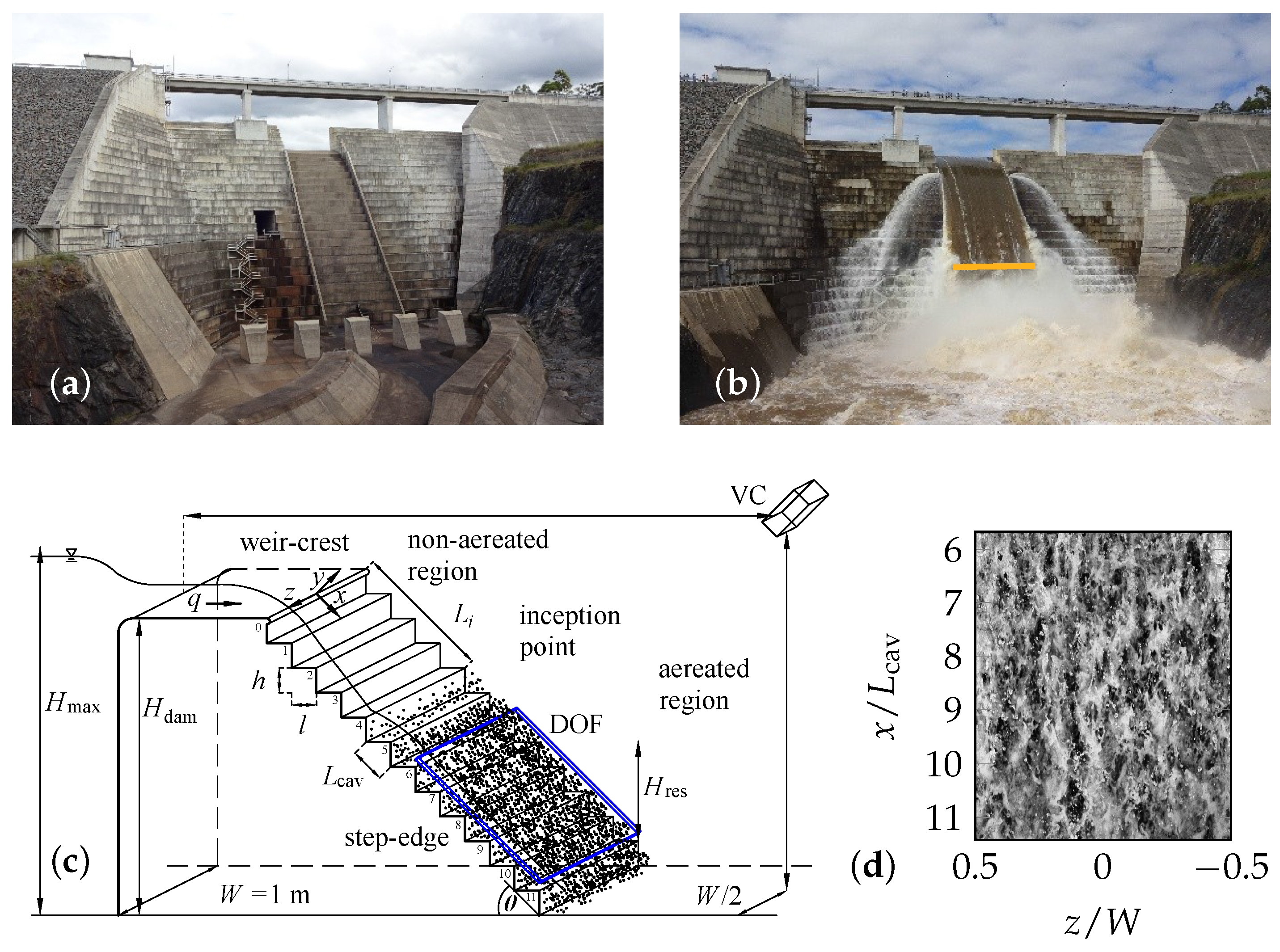
2.1. Prototype (Hinze Dam) and Laboratory (UQ) Stepped Spillway

Figure 1a,b show the Hinze Dam, which is a rock- and earth-fill dam located in the hinterland of the Gold Coast, Australia. The dam was constructed in 1976 and expanded in 1989 and in 2011, featuring an ungated ogee-crested stepped spillway with step height of h = 1.2 m, step width $W\approx$ 10 m, slope $\theta$ = 51.3${}^{\circ }$ and discharge capacity of >2500 m${}^3$/s. The dam’s stilling basin is equipped with large concrete baffle blocks and guide vanes to facilitate energy dissipation and to direct the released flows. In March 2017, a major spill with a specific water discharge of $q_w$ ≈ 27 m${}^2$/s and an annual exceedance probability of AEP ≈ 1% occurred (Figure 1b). Drone videos of this event were obtained from a citizen scientist [27], who authorized their usage for research purposes.

Laboratory experiments were performed in a physical model of a stepped spillway (Figure 1c,d) at the University of Queensland (UQ). The test section consisted of a broad-crested weir, followed by a stepped section with 12 plywood steps of 1 m width (W), 0.1 m height (h) and 0.1 m length (l), yielding a symmetrical cavity shape and a slope of $\theta$ = 45${}^{\circ }$ (Figure 1a), see also Zhang and Chanson [28]. The cavity length was $L_{\mathrm{cav}}=0.1\times \sqrt{2}$ m and the step numbering and configurations are shown in Figure 1c, together with the definition of relevant parameters. Pointer gauges in centerline were used to locally measure flow depths upstream of the broad-crested weir and above the crest with an accuracy of ±1 mm. A high-speed video camera was mounted on top of the stepped chute (Figure 1c,d), remotely measuring the surface of the air–water flows (Section 2.2). For validation purposes, air–water flow properties throughout the air–water column were measured intrusively with a dual-tip phase-detection conductivity probe in channel centerline (Section 2.3).

The laboratory experiments were conducted for transition ($d_c/h$ = 0.5 and 0.8) and skimming flows ($d_c/h$ = 1.1), where $d_c$ is the critical flow depth $d_c={(q^2/g)}^{1/3}$. The transition flow regime occurred at intermediate discharges and was characterized by falling nappes and recirculating water pools within the step cavities [29], while the skimming flow regime was more stable, characterized by recirculation motions in the step cavities [30]. The prototype flow conditions on the stepped spillway of Hinze Dam corresponded to the skimming flow regime ($d_c/h$ ≈ 2.6), with a clearly visible inception point of free-surface aeration (Figure 1b).

Table 1. Present flow conditions; note that intrusive phase-detection probe measurements for $d_c/h=$ 0.5 and 0.8 were presented in Kramer and Chanson [29]; TRA = transition flow; SK = skimming flow.

${\mathit{d}}_{\mathit{c}}/\mathit{h}$	${\mathit{q}}_{\mathit{w}}$	${\mathit{U}}_{\mathit{c}}$	${\mathit{F}}_{*}$	$\mathit{\theta }$	Regime	${\mathit{L}}_{\mathit{i}}$/${\mathit{L}}_{\mathbf{cav}}$	${\mathit{L}}_{\mathit{i}}$/k	$\mathit{Re}$	Comment
(−)	(m${}^{\mathbf{2}}$/s)	(m/s)	(−)	(${}^{\circ }$)	(−)	(−)	(−)	(−)
0.5	0.032	0.68	0.65	45	TRA	2	4	$3.2\times {10}^4$	Laboratory scale
0.8	0.067	0.87	1.35	45	TRA	2	4	$6.7\times {10}^4$	broad-crested weir
1.1	0.110	1.02	2.22	45	SK	4	8	$1.1\times {10}^5$	clear water
2.6	≈17.21		7.18	51.3	SK	12	24.6	$1.7\times {10}^7$	Prototype scale
									ogee-crested weir
									turbid water

summarizes flow conditions for both laboratory and prototype scale measurements, including the Reynolds number ($Re=q/\nu$; with $\nu$ being the kinematic viscosity of water), the flow regime, the roughness height ($k=hcos\theta$) and the dimensionless Froude number, defined in terms of the step roughness [7,31,32]:

$$F_{\star }=q_w/\sqrt{g{k}^{3}sin\theta }$$

(1)

where g is the gravitational acceleration. The Reynolds numbers of the laboratory and prototype stepped chutes differed by two to three orders of magnitude.

2.2. Cameras and Signal Processing

For the laboratory experiments, a Phantom v2011 high-speed video camera was used to film image sequences (1200 × 800 pixels resolution) of the aerated flow region from a top-view perspective. The camera was mounted above the stepped test section and aligned perpendicular to the chute’s pseudo-bottom, formed by the outer step edges (Figure 1a). All sampling sequences were recorded with a frame rate f = 2000 Hz for a sampling duration T = 15 s, fulfilling recommended sampling parameters for optical flow (OF) estimations in air–water flows [26]. The camera was equipped with an AF Nikkor 50 mm lens, allowing the recording of images with a small degree of distortion (Figure 1d). The focus of the camera was set to the upper flow region and the depth of field (DOF) was approximately stretching from y = 40 mm to 60 mm, measured vertically from the pseudo-bottom. The DOF corresponded to $y/d_c$ = 0.8 to 1.2 for $d_c/h$ = 0.5, to $y/d_c$ = 0.5 to 0.75 for $d_c/h$ = 0.8 and to $y/d_c$ = 0.36 to 0.54 for $d_c/h$ = 1.1. Additional videos were taken with a Casio EX-10 camera, which were used to determine the location of the inception point of free-surface aeration. The sampling rate and the sampling duration of these sequences were f = 120 Hz and $T=$ 30 s, respectively.

In March 2017, a citizen scientist filmed the Hinze Dam prototype spill (Figure 1b) with a DJI phantom drone (1200 × 512 pixels resolution) and the video footage (f = 30 Hz) was made available for the present research [27]. Herein, the recordings were post-processed and the video was cut into individual sequences ($T\approx 6$ s) with a stable top-view perspective, where the camera was perpendicular to the pseudo-bottom of the stepped spillway.

The video signals (laboratory and prototype) were analyzed with the Farnebaeck method (Appendix A), which has recently attracted interest in the study of air–water flows due to its robustness [24]. This optical flow (OF) velocimetry technique provided instantaneous air–water surface velocities in streamwise ($u_{\mathrm{surf}}$) and transverse directions ($w_{\mathrm{surf}}$). As those estimates may still contain erroneous values, some additional filtering is required. Following Kramer et al. [33], two filtering routines were applied to the obtained velocity data, including (i) an image-gradient filter that discarded background movement [26] and (ii) a robust outlier cut-off (ROC) [34], aiming at the rejection of spikes. The ROC represents a simplification of the method of Goring and Nikora [35] and was applied to the velocity time series at each pixel. Combining the above criteria, an indicator function ($\gamma$) was defined for the ith realization as follows:

$${\gamma }_i(x,z)=\{\begin{array}{ll}1& \mathrm{if}{I}_{i,m}(x,z)>g_t\mathrm{or}\mathrm{if}\frac{|u_{i,\mathrm{surf}}-\mathrm{MED}\left(u_{\mathrm{surf}}\right)|}{1.483\times \mathrm{MAD}\left(u_{\mathrm{surf}}\right)}\le \sqrt{2lnn}\\ 0& \mathrm{otherwise}\end{array}$$

(2)

where $g_t$ is a gradient threshold (herein $g_t=10$ px${}^{-1}$), MED is the median operator, MAD is the median absolute deviation, $n=f\times T$ is the total number of realizations/video frames and $I_m$ is the image gradient magnitude, which was evaluated using the classic Sobel operator [36]. The ensemble-averaged optical flow surface velocities and their root mean square fluctuations ($rms$) were subsequently calculated as:

$${\overline{u}}_{\mathrm{surf}}=\frac{{\sum }_{i=1}^N{\gamma }_i{u}_{\mathrm{surf}}}{{\sum }_{i=1}^N{\gamma }_i};{\overline{w}}_{\mathrm{surf}}=\frac{{\sum }_{i=1}^N{\gamma }_i{w}_{\mathrm{surf}}}{{\sum }_{i=1}^N{\gamma }_i}$$

(3)

$$u_{\mathrm{surf},rms}^{\prime }=\sqrt{\frac{{\sum }_{i=1}^N{\left(u_{\mathrm{surf},i}-{\overline{u}}_{\mathrm{surf}}\right)}^2{\gamma }_i}{{\sum }_{i=1}^N{\gamma }_i}};w_{\mathrm{surf},rms}^{\prime }=\sqrt{\frac{{\sum }_{i=1}^N{\left(w_{\mathrm{surf},i}-{\overline{w}}_{\mathrm{surf}}\right)}^2{\gamma }_i}{{\sum }_{i=1}^N{\gamma }_i}}$$

(4)

2.3. Phase-Detection Probe and Signal Processing

Air–water flow properties (e.g., air concentrations c and interfacial velocities $u_{\mathrm{aw}}$) were measured intrusively using a phase-detection conductivity probe, consisting of two needle tips with inner electrodes with 0.25 mm diameter and outer casings of 0.8 mm diameter. The longitudinal separation of the probe tips was 4.7 mm and the probe had typical measurement uncertainties as presented in Kramer et al. [13] (Table 1). Signals were processed with the adaptive window cross-correlation (AWCC) technique [11,13,37], allowing a robust estimation of mean interfacial velocities and turbulence parameters. Note that the term interfacial refers to velocities of air–water interfaces; the interfacial velocity is representative for both phases if phase drift velocities are negligible, for further details see discussion in Kramer et al. [37]. To compensate previously overestimated turbulence levels due to inappropriate assumptions in signal processing (as discussed in Kramer et al. [37]) and to validate image-based air–water surface velocimetry, turbulence levels of measurements from Kramer and Chanson [29] were re-calculated following the approach of Kramer et al. [11,13].

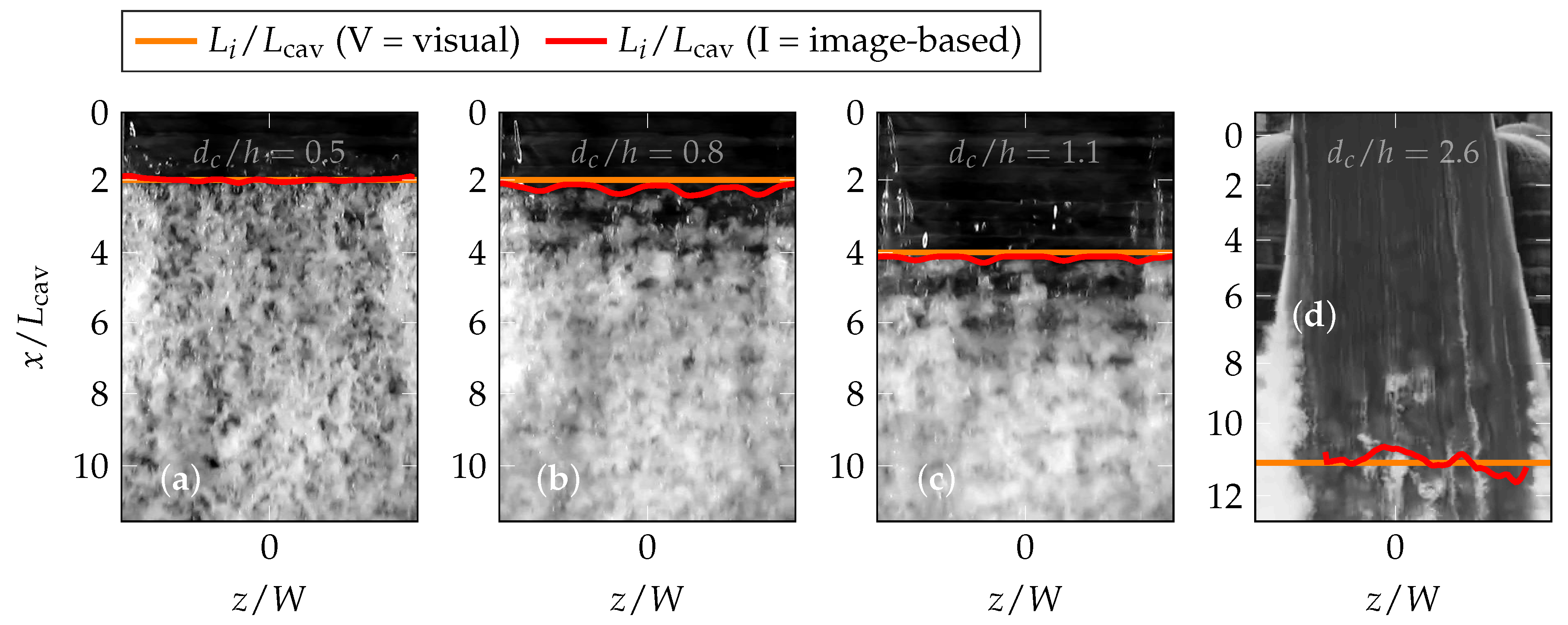
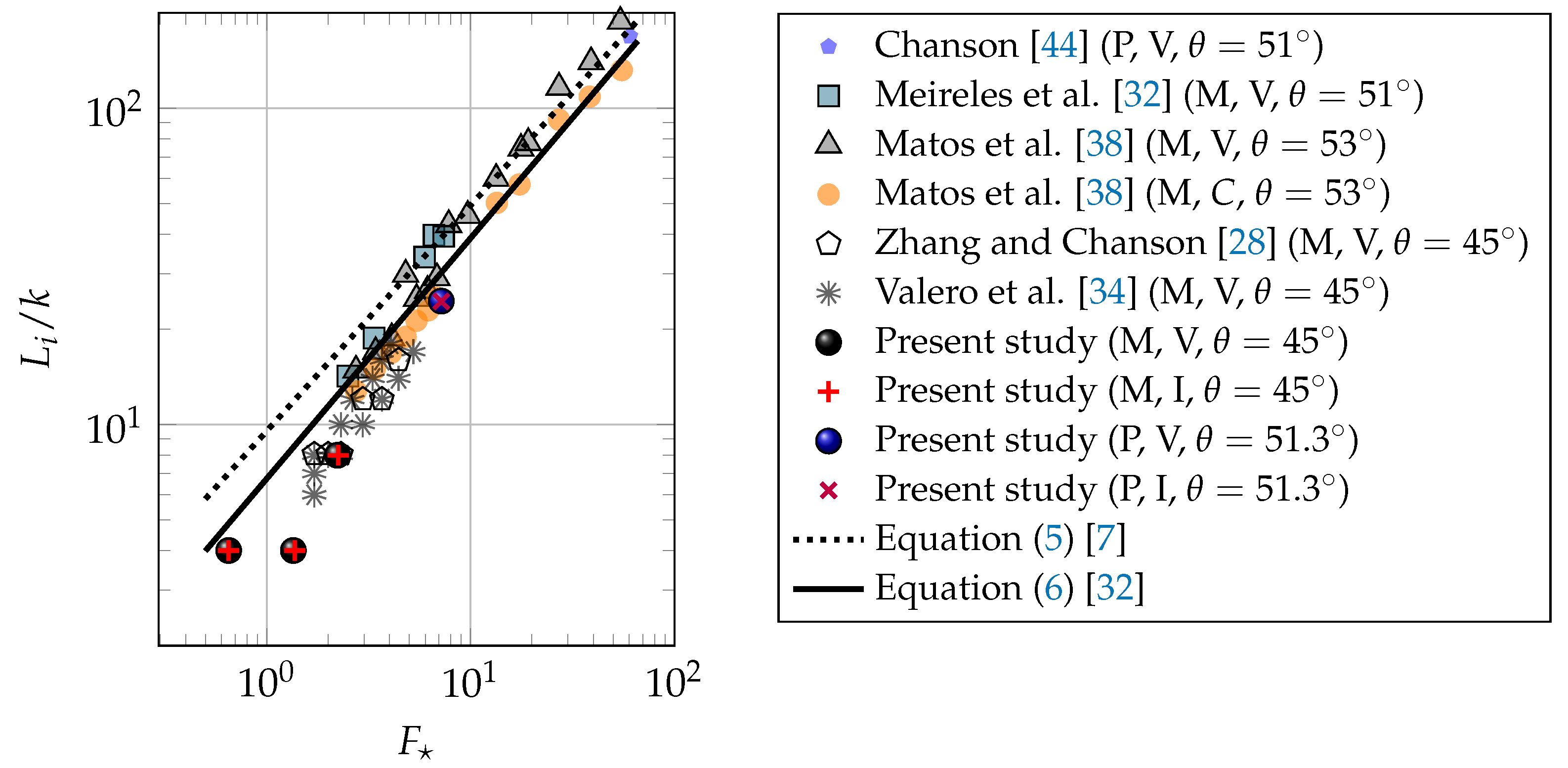
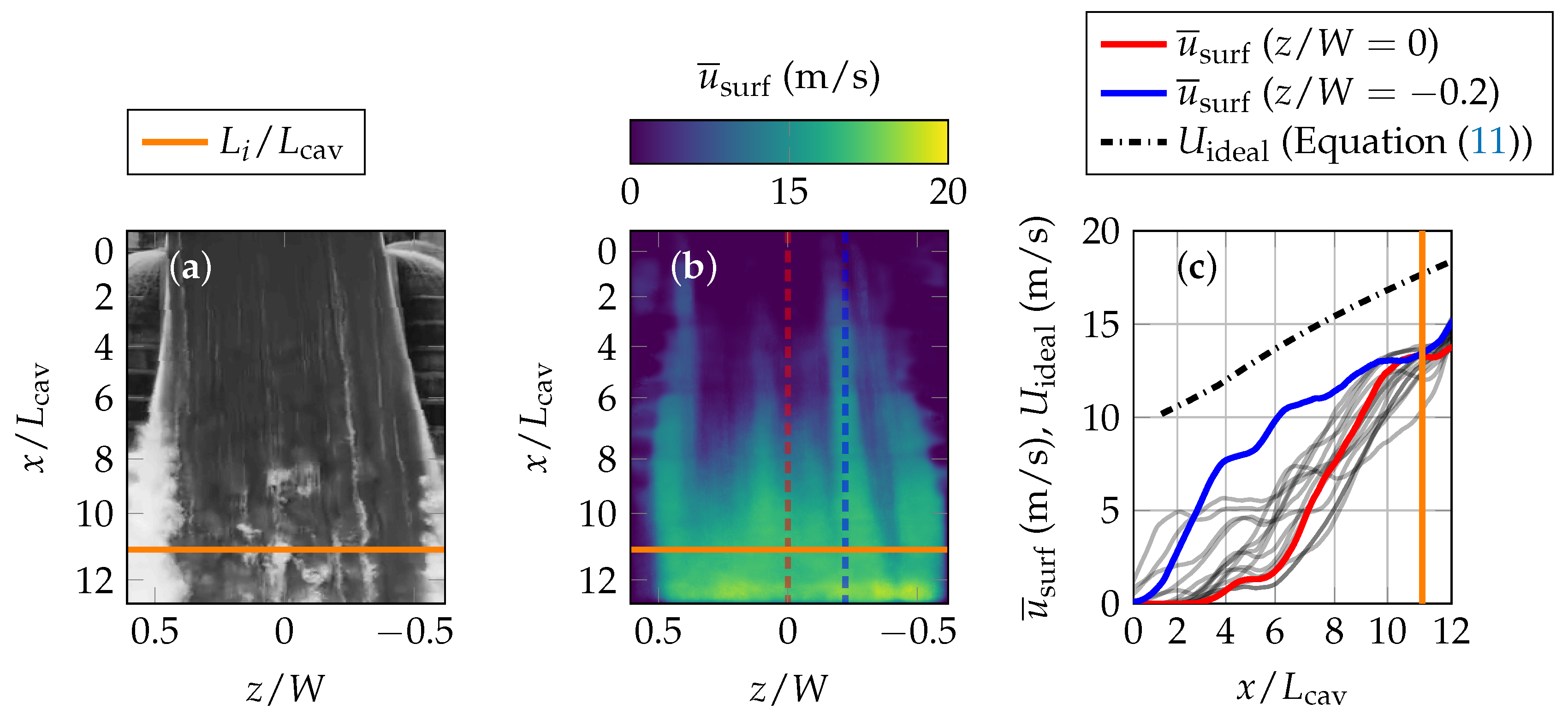
3. Results (1): Inception Point of Free-Surface Aeration

A key parameter for the characterization of high-velocity free-surface flows on chute spillways is the inception point of free-surface aeration. Researchers have used different methods to characterize this location, including visual observations through side-walls and from above as well as threshold levels in terms of depth-averaged air concentrations or air concentrations next to the pseudo-bottom [32,38]. Note that the inception point location is typically assessed as an average location, although its position fluctuates instantaneously. This process is linked with free-surface perturbations upstream of the inception point [39], as well as large-scale three-dimensional turbulent structures, which form within the step-cavities, leading to irregular burst and troughs of the free-surface [38,40].

Image-based analysis provides an alternative method to estimate the inception point of free-surface aeration from top-view perspective, similar to processing approaches for roller toe identification in hydraulic jumps [41] and breaking bores [42]. Herein, the inception point location was detected using a gradient-based algorithm, which consisted of the following steps: (i) extract raw image from the recorded image sequence, (ii) perform erosion and dilatation operations to reduce reflections and glares, (iii) evaluate the image gradient magnitude, (iv) perform time-averaging of the image gradient magnitude and detect the time-averaged inception point location based on a defined threshold. Figure 2 shows snapshots of the laboratory and prototype experiments, together with time-averaged inception point locations, determined visually (see also Figure 1b for the prototype flow) and via image-based analysis. Both methods demonstrated good agreement, thereby endorsing the application of the gradient-based algorithm. It is also seen that the image-based analysis provided more details and revealed the presence of 4–5 vortices across the width of the first aerated step cavities of the laboratory flume (Figure 2b,c). The video analysis of the Hinze Dam confirmed free-surface scars and large three-dimensional longitudinal vortical structures upstream of the inception point of free-surface aeration (Figure 1b and Figure 2d). Note that the image-based analysis of the prototype did not provide meaningful data next to the sidewalls, which was due to overtopping effects. Compared to the laboratory experiments, the waters at prototype scale were turbid, which may have caused minor differences in the estimated inception point locations. For example, the determination of aeration deeper in the water column at prototype scale was limited, while entrained air next to the free-surface was clearly distinguishable.

The present observations of the inception point locations are shown in Figure 3 together with selected previous inception point data on similar steep slopes, as well as empirical equations of Chanson [7] and Meireles et al. [32]:

$$L_i/k=9.719sin{\left(\theta \right)}^{0.0796}{\left(F_{\star }\right)}^{0.713}$$

(5)

$$L_i/k=6.74{\left(F_{\star }\right)}^{0.76}$$

(6)

The Hinze Dam data were in agreement with previous observations on selected prototype stepped spillways, while the laboratory data were in close agreement with inception point data of Zhang and Chanson [28] and Valero et al. [34], which were collected on the same stepped spillway using visual observations through the side wall. The data on the laboratory stepped chute appeared to indicate an earlier inception point when compared to several other laboratory studies with similar steep slopes. This difference may be linked to the particular inflow conditions, i.e., a steeply sloped chute downstream of a broad-crested weir with a downstream rounded edge [28] compared to ogee-crested weirs in previous studies of laboratory stepped spillways. Overall, the determined inception points demonstrated a reasonable agreement with previous studies irrespective of the scale of the observations, as previously reported in Meireles et al. [32] and Chanson et al. [43].

4. Results (2): Laboratory Stepped Spillway

This section presents the results of the laboratory experiments, including air concentrations, interfacial velocities, surface mean velocities, and velocity fluctuations, as well as a validation of optical surface flow velocimetry in high-velocity air–water flows.

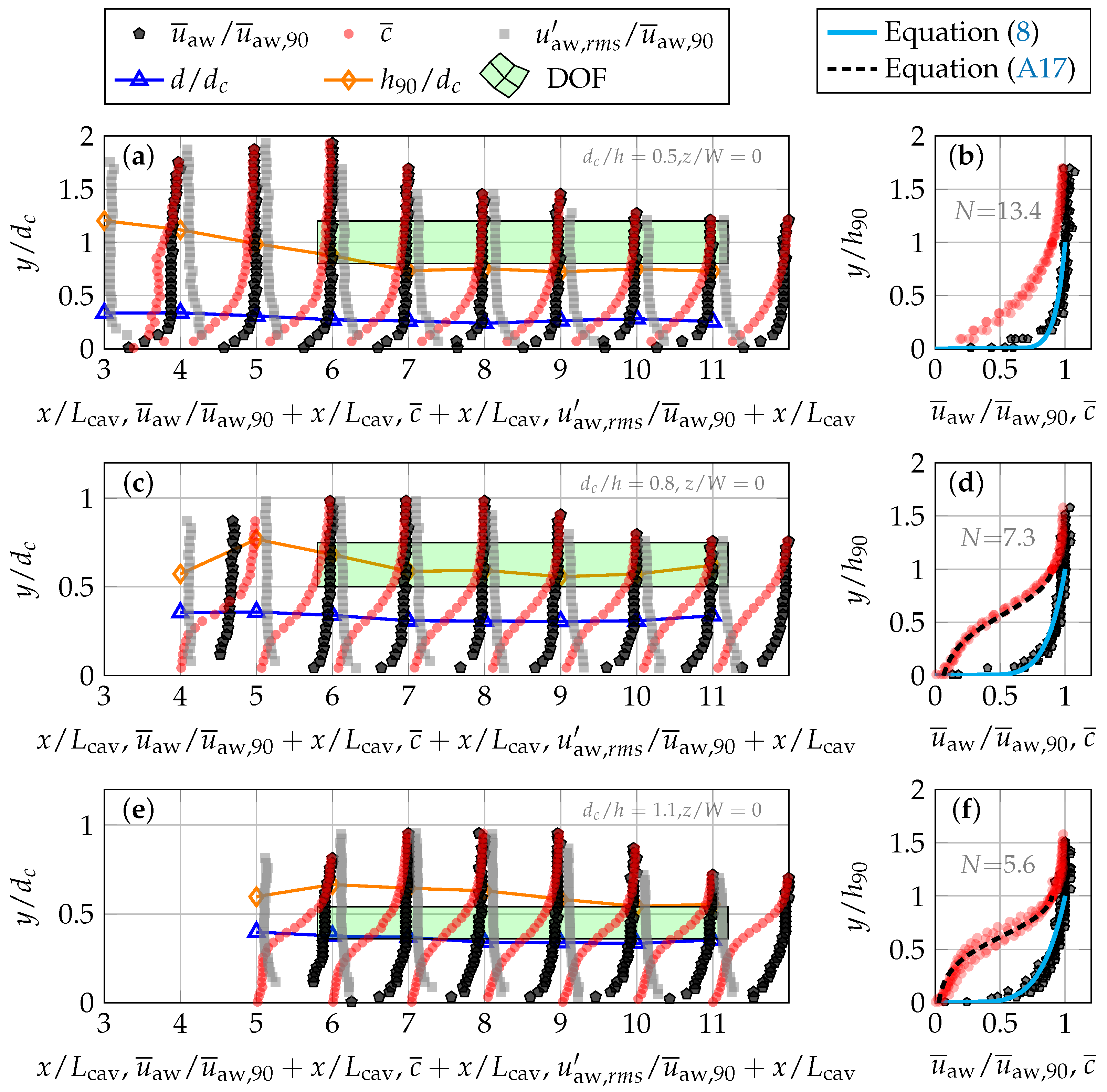
4.1. Air–Water Flow Properties

Air–water flow properties were measured intrusively with the conductivity probe in spillway centerline ($z/W=0$), providing local volumetric air concentrations, interfacial mean velocities (${\overline{u}}_{\mathrm{aw}}$), velocity fluctuations ($u_{\mathrm{aw},rms}^{\prime }$) and the equivalent clear water flow depth (d), defined as:

$$d={\int }_{y=0}^{h_{90}}(1-\overline{c})\mathrm{d}y$$

(7)

where the mixture flow depth $h_{90}$ corresponds to the elevation where $\overline{c}=0.9$, i.e., $h_{90}=h(\overline{c}=0.9)$.

Figure 4a,c,e show the evolution of air–water flow properties along the stepped chute for the three flow rates. Downstream of the inception point, the flows were rapidly varied and aeration occurred over a short distance, associated with flow bulking and strong splashing. Towards the downstream end of the chute, i.e., $x/L_{\mathrm{cav}}\approx$ 8 to 11, streamwise gradients of d and $h_{90}$ were small and the flows were gradually varied. The distribution of $\overline{c}$ followed typical S-shaped profiles, which were well described by semi-empirical solutions of the diffusion equation for air in water [45] (Table III-1), see Equation (A17) in Appendix C. Note that Equation (A17) was developed for skimming flows and its solution is, therefore, not shown in Figure 4b.

Interfacial velocities (${\overline{u}}_{\mathrm{aw}}$) increased with distance to the pseudo-bottom of the chute and were almost constant within the upper flow region, e.g., above $\overline{c}>$ 0.7 to 0.9 (Figure 4a,c,e). Turbulent fluctuations showed similarities to single-phase flows [46], implying that fluctuations were highest next to the chute invert and decreased exponentially with increasing mixture flow depth [11,13,37]. The DOFs (depth of field, DOF, shaded areas) of the camera are shown in Figure 4a,c,e. Because gradients of mean velocities and velocity fluctuations were small within the DOFs, it is hypothesized that the measured air–water surface velocities and fluctuations are representative for nearly uniform interfacial velocities and fluctuations in the upper flow region, for example at $h_{90}$. This implies that ${\overline{u}}_{\mathrm{surf}}\approx {\overline{u}}_{\mathrm{aw},90}$ and $u_{\mathrm{surf},rms}^{\prime }\approx u_{\mathrm{aw},90,rms}^{\prime }$, enabling a direct comparison between conductivity probe measurements and image-based surface velocimetry (Section 4.3).

The interfacial velocity distribution on spillways can be described with a power law [7,47,48]:

$$\frac{{\overline{u}}_{\mathrm{aw}}}{{\overline{u}}_{\mathrm{aw},90}}={\left(\frac{y}{h_{90}}\right)}^{\frac{1}{N}}$$

(8)

where ${\overline{u}}_{\mathrm{aw},90}$ is the interfacial velocity at $h_{90}$ and N is the power law exponent. The application of Equation (8) to aerated flows on smooth chutes was introduced by Cain and Wood [47] and later expanded to stepped chutes (e.g., [7,48]). Similar to single-phase flows (see [49]), a large range of power law exponents between $N\approx 4$ to 15 has been found applicable to aerated chute flows [50] (Figure 8), hinting that N depends on Reynolds number, relative roughness, chute slope and on the air concentration next to the chute invert. Takahashi and Ohtsu [50] proposed an empirical relationship for the power law exponent in skimming flows:

$$N=14{\theta }^{-0.65}h/d_c\left(\frac{100}{\theta }\frac{h}{d_c}-1\right)-0.041\theta +6.27\mathrm{for}{19}^{\circ }\le \theta \le {55}^{\circ }$$

(9)

where $\theta$ is in degrees. Equation (9) was evaluated for the present flow conditions, resulting in $N=13.4,7.3$ and 5.6 for $d_c/h$ = 0.5, 0.8, and 1.1. Figure 4b,d,f show a comparison of normalized interfacial velocity profiles in the gradually varied flow region ($x/L_{\mathrm{cav}}$ = 8 to 11), demonstrating that the exponent was reasonably estimated with Equation (9).

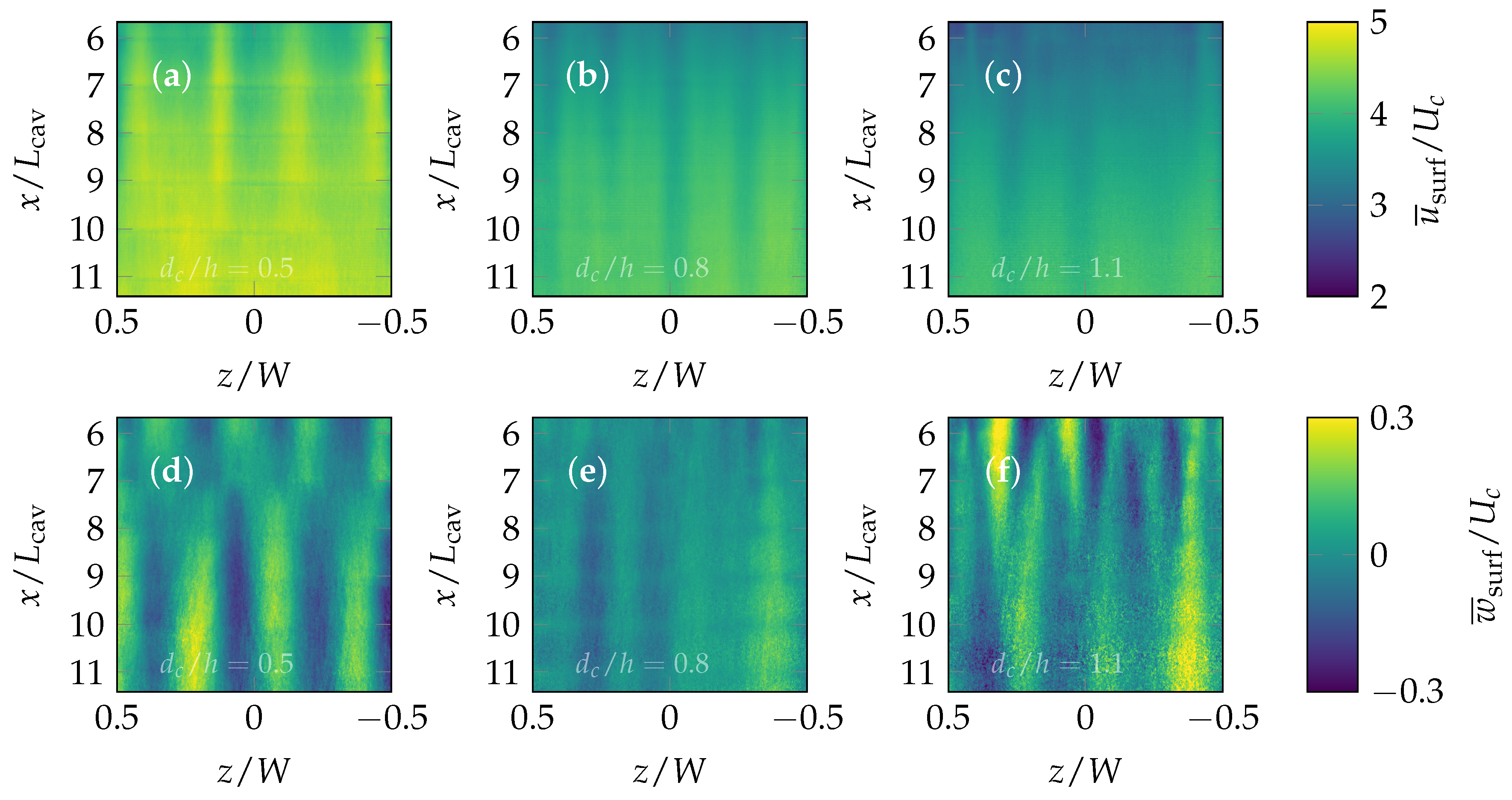
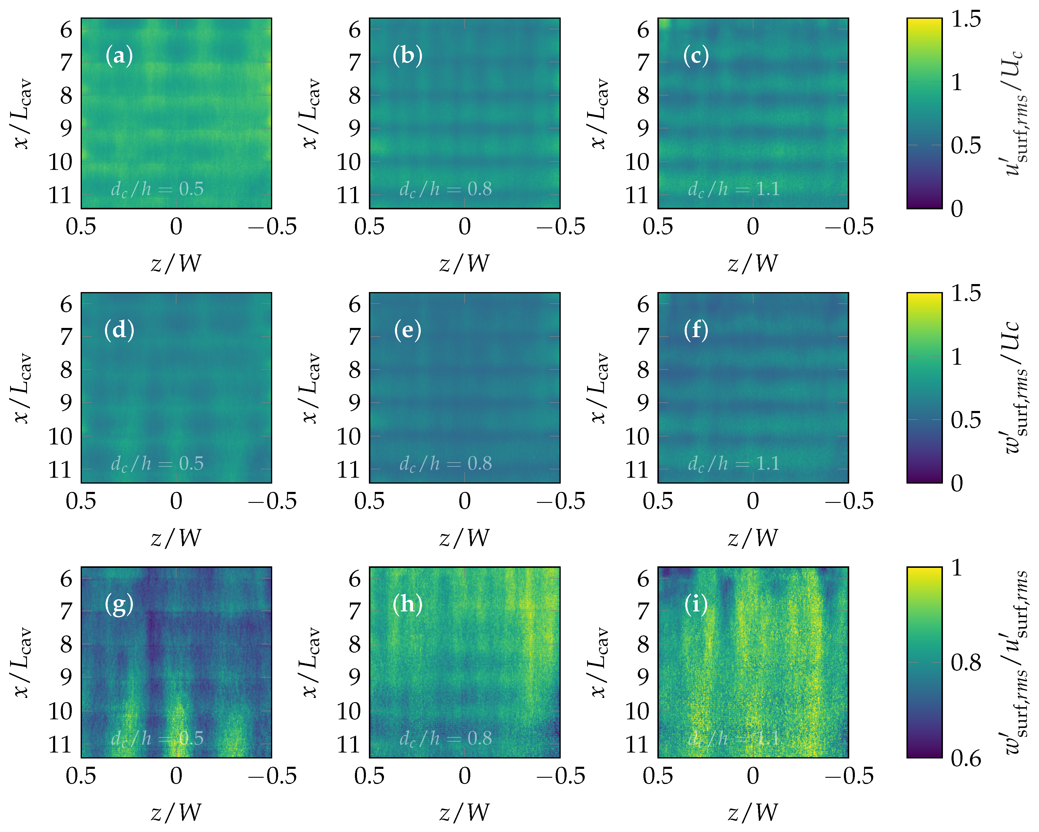
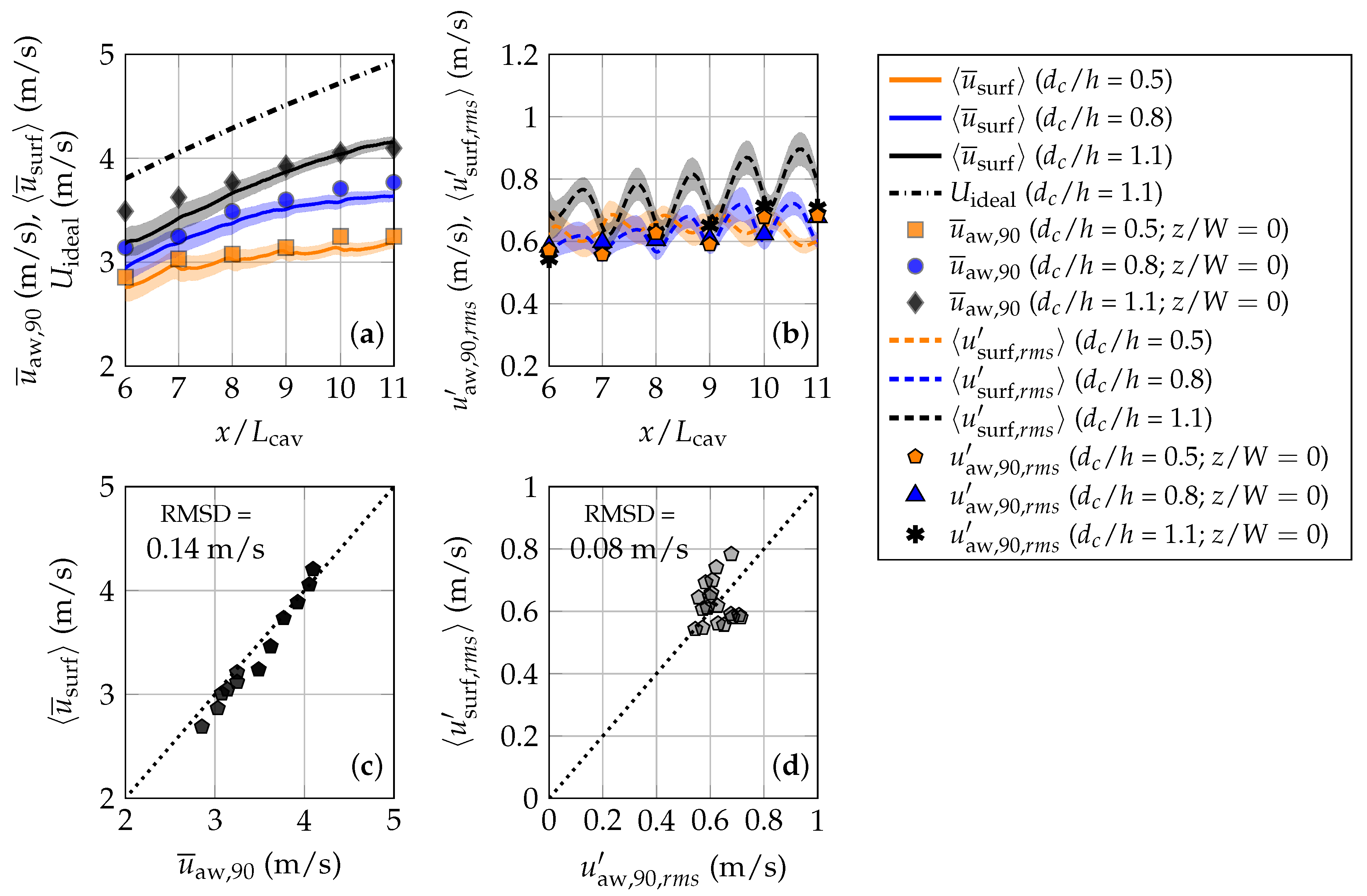
4.2. Surface Mean Velocities and Turbulence

Surface velocities of the aerated flow were estimated with the Farnebaeck method (Appendix A) and filtering using Equation (3). Mean velocities showed an accelerating flow along the chute (Figure 5a–c), implying that uniform flow conditions may not have been reached at its downstream end. Longitudinal streaks of slightly higher streamwise velocities were consistently observed. Stepped spillway flows are characterized by vortices within the step cavities and ejections of fluid lumps from the cavities into the overlying flows may explain the formation of the observed free-surface streaks. This was confirmed by visual observations, which revealed the presence of 4 to 5 vortices across one step-cavity for $d_c/h=$ 0.8 and 1.1. Note that these observations are also consistent with earlier numerical simulations [51].

Although transverse time-averaged velocities were much smaller than streamwise velocities, i.e., ${\overline{w}}_{\mathrm{surf}}<0.05\times {\overline{u}}_{\mathrm{surf}}$, they also showed distinct free-surface streaks (Figure 5d–f). The present observations of streamwise and transverse free-surface velocities with high-spatial resolution highlighted the strength of the remote sensing method to provide novel insights into the spatial heterogeneity of air–water flows, inferring their complex underlying flow structure. Currently, 3-dimensional velocity measurements of stepped spillway flows are missing in both, non-aerated and aerated flow regions, and the formation of vortical structures within step cavities, as well as their interaction with the flow above the pseudo-bottom remain poorly understood.

Turbulent stresses of the air-water surface were evaluated based upon instantaneous velocity measurements and filtering with Equation (4). Both streamwise and transverse velocity fluctuations increased in magnitude along the stepped chute for $d_c/h=0.5$, while the increase was smaller for the larger flow rates $d_c/h=0.8$ and 1.1. The streamwise velocity fluctuations $u_{rms,\mathrm{surf}}^{\prime }$ (Figure 6a–c) were consistently larger than the transverse fluctuations $w_{rms,\mathrm{surf}}^{\prime }$ (Figure 6d–f) for all experiments. Figure 6g–i show the relation of transverse and longitudinal air–water surface velocity fluctuations. For $d_c/h=0.5$, it is seen that the free-surface streaks had relatively large transverse velocity fluctuations, while the relation was between $w_{\mathrm{surf},rms}^{\prime }/u_{\mathrm{surf},rms}^{\prime }\approx 0.7$ to 0.9 for the two larger flow rates.

Nezu and Nakagawa [52] proposed models for the bed-normal distribution of turbulent fluctuations in single-phase open channel flows, indicating that the relation of transverse and streamwise turbulent fluctuations is approximately [52] (Equation (4.7)):

$$w_{rms}^{\prime }/u_{rms}^{\prime }=0.71$$

(10)

The similarity of the present relationship in surface velocities with those of Nezu and Nakagawa [52] indicates that established correlations for single-phase flows may be applicable to multiphase air–water flows, while additional observations are required for confirmation. For all properties and flow conditions shown in Figure 6, the step edges were visible in the result figures as horizontal lines. This was caused by less brightness variance of the flow directly above the step edges. It is anticipated that such effects may not be visible at prototype scale due to (i) the underestimation of air entrainment at laboratory scale, (ii) larger flow depths at prototype scale, and (iii) high turbidity leading to a decrease in the water’s transparency under real-world conditions (see Figure 1b).

4.3. Validation of Surface Velocimetry in Air–Water Flows

To validate the surface velocimetry in air–water flows, present results were compared with corresponding conductivity probe data in channel centerline ($z/W=0$) at $h_{90}$. Figure 7a shows the comparison of the longitudinal evolution of streamwise air–water free-surface velocities $\langle {\overline{u}}_{\mathrm{surf}}\rangle$, spatially averaged over the width of the chute (z), with interfacial velocities (${\overline{u}}_{\mathrm{aw},90}$) for all flow conditions. The spatial variability of velocities ${\overline{u}}_{\mathrm{surf}}$ across the chute width is visualized as shaded area and represents the velocity standard deviation. This transverse variability decreased towards the downstream end of the stepped chute (Figure 7a).

Mean streamwise surface velocities and corresponding interfacial velocities at $h_{90}$ were in close agreement $\langle {\overline{u}}_{\mathrm{surf}}\rangle$≈${\overline{u}}_{\mathrm{aw},90}$ and the root mean square deviation (RMSD) between these two velocities was 0.14 m/s (Figure 7c). Velocities just downstream of the inception point of free-surface aeration, e.g., at $x/L_{\mathrm{cav}}\approx 6$ to 7, were less accurately predicted with the optical flow velocimetry, which is believed to be linked to smaller flow aeration in this part of the flow (see Figure 2a–c). In Figure 7a, the measured velocities were also compared with frictionless velocities above the pseudo-bottom:

$$U_{\mathrm{ideal}}=\sqrt{2g\left(H_{\max }-y-dcos\theta \right)}$$

(11)

The comparison of $U_{\mathrm{ideal}}$ with the interfacial velocities at $h_{90}$ showed that ${\overline{u}}_{\mathrm{aw},90}/U_{\mathrm{ideal}}\approx$ 0.7 to 0.9, providing an indirect estimate of the friction loss along the stepped chute. Lastly, streamwise air–water surface velocity fluctuations, averaged over the width of the flume (shaded areas represent their standard deviation across the flume’s width), were in good agreement with the corresponding streamwise interfacial velocity fluctuations in centerline at $h_{90}$ (Figure 7b), indicating that $u_{\mathrm{surf},rms}^{\prime }\approx u_{\mathrm{aw},90,rms}^{\prime }$. The comparison of the two velocity approaches revealed a deviation RMSD = 0.08 m/s (Figure 7d).

To summarize, the comparative analysis of image-based air–water surface velocimetry with interfacial velocities revealed a close agreement between the two techniques. The measured air–water surface velocities approximated the interfacial velocities and their fluctuations at the mixture flow depth $h_{90}$ accurately, validating air–water velocimetry as a new method for the recording of air-water surface velocities in fully-aerated high-velocity flows.

5. Results (3): Surface Velocities at Prototype Scale

Optical flow velocimetry was applied to drone video footage of an overtopping event of Hinze Dam in March 2017. Figure 8a presents an exemplary single frame of the drone video, showing that the upper part of the spillway flow ($x/L_{\mathbf{cav}}\approx 0$ to 6) was non-aerated and characterized by free-surface scars and longitudinal streaks, which have previously been reported in similar high-velocity flows on prototype stepped spillways [53,54].

Further downstream, approximately at $x/L_{\mathrm{cav}}>8$, the flows became intermittently aerated, while the inception point of free-surface aeration was located at $L_i\approx 11L_{\mathrm{cav}}$ (Figure 2d and Figure 8). Note that the flows were also aerated at the edges of the spillway and along free-surface streaks in the non-aerated region (Figure 8a). Using optical flow velocimetry, velocity estimations were obtained in regions with intermittent surface aeration as shown in Figure 8b. The time-averaged streamwise air–water surface velocities ${\overline{u}}_{\mathrm{surf}}$ provided an estimate of the overall velocity magnitude, which reached up to 15 m/s, highlighting the substantially larger scale of the prototype flow observations compared to typical laboratory measurements.

Figure 8c shows the development of streamwise velocities along the chute for 15 different equally-spaced transverse locations ranging between $z/W$ = −0.5 to 0.5. Two velocity profiles are highlighted in blue and red, representing the centerline ($z/W=0$) and the location of a prominent streak along the non-aerated region ($z/W=-0.2$). For clarity, these two sections are shown as dashed lines in Figure 8b. The profiles of the mean streamwise velocities along the chute showed some data scatter in locations with no flow aeration ($x/L_{\mathrm{cav}}\lesssim 6$), while all profiles converged in the aerated region for $x/L_{\mathrm{cav}}\gtrsim 11$. The streamwise velocity profile in centerline represented a typical velocity profile, which appeared to suggest an underestimation of ${\overline{u}}_{\mathrm{surf}}$ in the non-aerated region due to missing brightness information and surface tracers, while the data in the aerated flow region appeared to be meaningful. In contrast, the velocity profile along the aerated streak ($z/W=-0.2$) was of better quality and allowed a more realistic estimation of free-surface velocities in the non-aerated flow region.

To check the validity of the velocity estimations, the idealized frictionless velocity $U_{\mathrm{ideal}}$ was calculated using Equation (11), where the water flow depth in the developing flow region was approximated with a solution of the backwater equation for stepped spillways [55] (Equations (5) and (9)). Although the streamwise free-surface velocities were substantially lower in the non-aerated flow region (apart from the streak along $z/W=-0.2$), the ratio of surface velocities to ideal velocities was ${\overline{u}}_{\mathrm{surf}}/U_{\mathrm{ideal}}\approx$ 0.8 for $x/L_{\mathrm{cav}}>10$, which was similar to the ratio of ${\overline{u}}_{\mathrm{surf}}$ and $U_{\mathrm{ideal}}$ in the laboratory experiments (see Section 4.3). These present findings must be further evaluated in prototype measurements with recordings of a larger area of aerated flows.

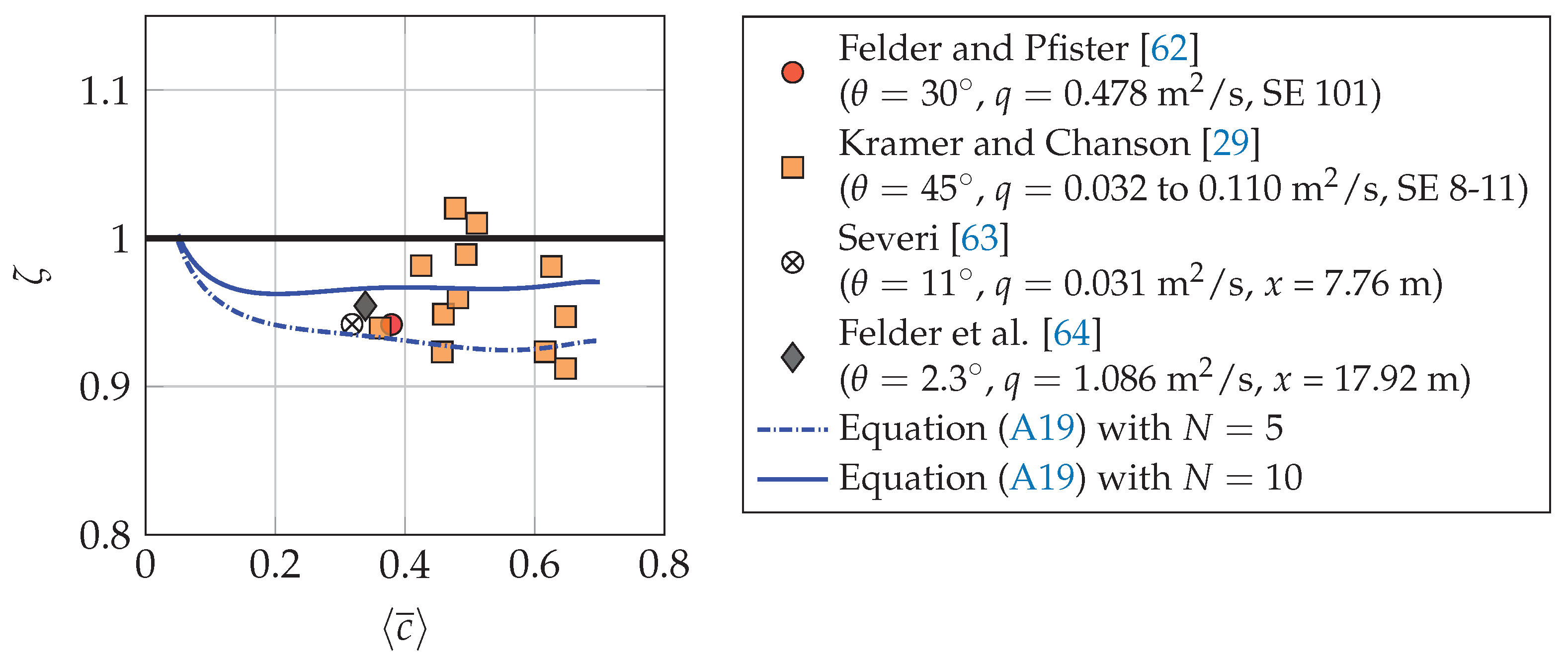
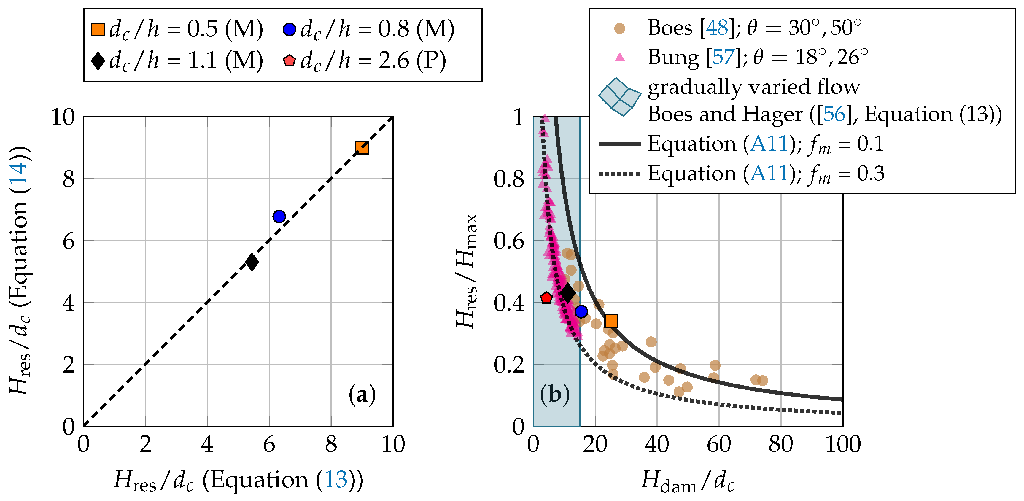
6. Discussion: Remote Estimation of Residual Energy

The residual energy at the downstream end of a spillway (Figure 1c) is a key parameter for the design of energy dissipators, such as stilling basins, and is commonly calculated in terms of the equivalent clear water flow depth and the mean water velocity $\langle {\overline{u}}_w\rangle$:

$$\begin{array}{ccc}\hfill H_{\mathrm{res}}& =& dcos\theta +\alpha \frac{{\langle {\overline{u}}_w\rangle }^2}{2g}\hfill \end{array}$$

(12)

$$\begin{array}{ccc}& =& dcos\theta +\alpha \frac{{\left(\frac{1}{d}{\int }_{y=0}^{h_{90}}{\overline{u}}_{\mathrm{aw}}\left(1-\overline{c}\right)\mathrm{d}y\right)}^2}{2g}\hfill \end{array}$$

(13)

where $\alpha$ is the kinetic energy correction factor and the right-hand side of Equation (13) may be evaluated solely based on intrusively measured air–water flow properties. A remote sensing expression for the residual energy can be written as (Appendix B):

$$H_{\mathrm{res}}=\frac{q_w(N+1)}{\zeta \langle {\overline{u}}_{\mathrm{surf}}\rangle N}cos\theta +\frac{\alpha }{2g}{\left(\zeta \frac{\langle {\overline{u}}_{\mathrm{surf}}\rangle N}{N+1}\right)}^2$$

(14)

where it was assumed that $\langle {\overline{u}}_{\mathrm{surf}}\rangle \approx {\overline{u}}_{\mathrm{aw},90}$ (Figure 7a) and $\zeta$ is a correction factor (Appendix C), accounting for differences between mean interfacial and mean water velocities.

For the laboratory experiments, the residual energy at the last step edge ($x/L_{\mathrm{cav}}=11$; Figure 1c) was computed for the three flow conditions using both, intrusive air–water flow measurements (Equation (13) and the remote sensing methodology (Equation (14)). Equation (14) was evaluated using correction factors $\alpha =1.1$ [56], $\zeta$ calculated with Equation (A19), power law coefficients after Equation (9) and measured water discharges (Table 1). Figure 9a shows the comparison of residual energies evaluated with the two methods, demonstrating an excellent agreement between intrusive air-water flow measurements and the proposed remote sensing approach.

Subsequently, the remote sensing methodology was applied to the prototype flow and the residual energy at $x/L_{\mathrm{cav}}=12$ was estimated using Equation (14) with $\langle {\overline{u}}_{\mathrm{surf}}\rangle$ = 13.9 m/s (Figure 8c), $\alpha =1.1$, $\zeta =0.95$, $N=4.06$ (Equation (9)) and $q_w$ = 17.21 m${}^2$/s (Table 1), leading to $H_{\mathrm{res}}$ = 7.39 m. Figure 9b shows a comparison of the present results with previous literature data, where an analytical solution of the residual energy (Equation (A11)) was added for completeness, with $H_{\max }$ being the total head at the weir crest. It is seen that the laboratory measurements compared well with the previous study of Boes [48] ($\theta ={30}^{\circ }$ to ${50}^{\circ }$), while the estimated residual energy of the prototype spill was smaller than anticipated. This was most likely caused by the fact that the measurement location ($x/L_{\mathrm{cav}}=12$) was upstream of the uniform flow region, confirmed through an empirical equation for attainment of flow uniformity by Boes and Hager [56] (Equation (13)). Other reasons may include the applicability of Equation (9) to prototype flows, which requires further verification.

Overall, Equation (14) offers novel opportunities to remotely estimate the energy dissipation in aerated flows on prototype structures, thereby providing the basis for a real-time monitoring framework and for future design and safety improvements (“the field becomes the laboratory”) of water conveyance infrastructure.

7. Conclusions

This study presents a proof of concept to remotely estimate air–water surface velocities and associated parameters in aerated flows down laboratory and prototype chutes. Detailed laboratory investigations comprised top-view video observations and intrusive air–water flow measurements. The comparative analysis of mean air–water surface velocities and velocity fluctuations with corresponding interfacial velocities showed a close agreement in the upper flow region (e.g., $h_{90}$), validating surface velocimetry as a novel method to remotely measure velocity statistics. Based upon these observations, an expression for the remote estimation of the residual energy was developed and successfully validated against traditional approaches using phase-detection intrusive measurements. These advances allow to remotely assess important design parameters of hydraulic infrastructure.

Image-based velocimetry was also applied to drone video footage of the spilling Hinze Dam (Australia), a major dam with a stepped chute as conveyance structure. The analysis of the remote video recordings highlighted the method’s suitability and provided proof of concept for image-based velocimetry in high-velocity air–water flows at prototype scale. Due to missing brightness information upstream of the inception point of free-surface aeration, velocities were underestimated in the non-aerated region of the chute flows, while the data in the aerated flow region were of good quality.

Overall, this study provided an important first step towards real-world, real-time monitoring of aerated flows in hydraulic structures, making use of a crowdsourced drone footage. It is anticipated that the present methodology will contribute towards (i) resolving long-standing research questions on scale effects in air–water flows, (ii) an improved design of water conveyance infrastructure, including spillways and other energy dissipation structures, and (iii) future developments in remote sensing of real-world aerated flows.

References

1. Ho, M.; Lall, U.; Allaire, M.; Devineni, N.; Kwon, H.H.; Pal, I.; Raff, D.; Wegner, D. The future role of dams in the United States of America. Water Resour. Res. 2017, 53, 982–997. [Google Scholar] [CrossRef]
2. Frizell, K.W.; Frizell, K.H.; Einhellig, R.F.; Fielder, W.R.; Matos, J. Guidelines for Hydraulic Design of Stepped Spillways; Hydraulic Laboratory Report HL-2015-05; U.S. Department of the Interior, Bureau of Reclamation: Denver, CO, USA, 2015.
3. Machado, B.P. Technical Advancements in Spillway Design—Progress and Innovations from 1985 to 2015, ICOLD Bulletin 172. 2016.
4. Chanson, H. Stepped Spillway Flows and Air Entrainment. Can. J. Civ. Eng. 1993, 20, 422–435. [Google Scholar] [CrossRef] [Green Version]
5. Kramer, M.; Felder, S.; Hohermuth, B.; Valero, D. Drag reduction in aerated chute flow: Role of bottom air concentration. J. Hydraul. Eng. 2021. [Google Scholar] [CrossRef]
6. Wood, I. Air Entrainment in Free-Surface Flows; IAHR Hydraulic Structures Manual No. 4; Hydraulic Design Considerations, Balkema Publ.: Rotterdam, The Netherlands, 1991. [Google Scholar]
7. Chanson, H. Air Bubble Entrainment in Free-Surface Turbulent Shear Flows; Academic Press: San Diego, CA, USA, 1996. [Google Scholar]
8. Valero, D.; Bung, D.B. Reformulating self-aeration in hydraulic structures: Turbulent growth of free surface perturbations leading to air entrainment. Int. J. Multiphase Flow 2017, 100, 127–142. [Google Scholar] [CrossRef]
9. Chanson, H.; Toombes, L. Air-water flows down stepped chutes: Turbulence and flow structure observations. Int. J. Multiphase Flow 2002, 28, 1737–1761. [Google Scholar] [CrossRef] [Green Version]
10. Felder, S.; Chanson, H. Phase-detection probe measurements in high-velocity free-surface flows including a discussion of key sampling parameters. Exp. Ther. Fluid Sci. 2015, 61, 66–78. [Google Scholar] [CrossRef]
11. Kramer, M.; Valero, D.; Chanson, H.; Bung, D.B. Towards reliable turbulence estimations with phase-detection probes: An adaptive window cross-correlation technique. Exp. Fluids 2019, 60, 2. [Google Scholar] [CrossRef]
12. Scheres, B.; Schuettrumpf, H.; Felder, S. Flow Resistance and Energy Dissipation in Supercritical Air-Water Flows Down Vegetated Chutes. Water Resour. Res. 2020, 56. [Google Scholar] [CrossRef] [Green Version]
13. Kramer, M.; Hohermuth, B.; Valero, D.; Felder, S. Best practices for velocity estimations in highly aerated flows with dual-tip phase-detection probes. Int. J. Multiphase Flow 2020, 126, 103228. [Google Scholar] [CrossRef] [Green Version]
14. Cain, P. Measurements within Self-Aerated Flow on a Large Spillway. Ph.D. Thesis, University of Canterbury, Christchurch, New Zealand, 1978. [Google Scholar]
15. Hohermuth, B.; Boes, R.; Felder, S. High-velocity air-water flow measurements in a prototype tunnel chute—Scaling of void fraction and interfacial velocity. J. Hydraul. Eng. 2021. [Google Scholar] [CrossRef]
16. Muste, M.; Fujita, I.; Hauet, A. Large-scale particle image velocimetry for measurements in riverine environments. Water Resour. Res. 2008, 44, W00D19. [Google Scholar] [CrossRef] [Green Version]
17. Tauro, F.; Piscopia, R.; Grimaldi, S. Streamflow Observations From Cameras: Large-Scale Particle Image Velocimetry or Particle Tracking Velocimetry? Water Resour. Res. 2017, 53, 374–394. [Google Scholar] [CrossRef] [Green Version]
18. Costa, J.E.; Spicer, K.R.; Cheng, R.T.; Haeni, F.P.; Melcher, N.B.; Thurman, M.T. Measuring stream discharge by non-contact methods: A proof-of-concept experiment. Geophys. Res. Lett. 2000, 27, 553–556. [Google Scholar] [CrossRef]
19. Johnson, E.D.; Cowen, E.A. Remote monitoring of volumetric discharge employing bathymetry determined from surface turbulence metrics. Water Resour. Res. 2016, 52, 2178–2193. [Google Scholar] [CrossRef] [Green Version]
20. Paul, J.D.; Buytaert, W.; Sah, N. A Technical Evaluation of Lidar-Based Measurement of River Water Levels. Water Resour. Res. 2020, 56. [Google Scholar] [CrossRef] [Green Version]
21. Bung, D. Non-intrusive detection of air-water surface roughness in self-aerated chute flows. J. Hydraul. Res. 2013, 51, 322–329. [Google Scholar] [CrossRef]
22. Zhang, G.; Valero, D.; Bung, D.; Chanson, H. On the estimation of free-surface turbulence using ultrasonic sensors. Flow Meas. Instru. 2018, 60, 171–184. [Google Scholar] [CrossRef] [Green Version]
23. Kramer, M.; Chanson, H.; Felder, S. Can we improve the non-intrusive characterisation of high-velocity air-water flows? Application of LIDAR technology to stepped spillways. J. Hydraul. Res. 2019, 171–184. [Google Scholar]
24. Bung, D.; Valero, D. Optical flow estimation in aerated flows. J. Hydraul. Res. 2016, 54, 575–580. [Google Scholar] [CrossRef]
25. Zhang, G.; Chanson, H. Application of local optical flow methods to high-velocity free-surface flows: Validation and application to stepped chutes. Exp. Ther. Fluid Sci. 2018, 90, 186–199. [Google Scholar] [CrossRef] [Green Version]
26. Kramer, M.; Chanson, H. Optical flow estimations in aerated spillway flows: Filtering discussion on sampling parameters. Exp. Ther. Fluid Sci. 2019, 103, 318–328. [Google Scholar] [CrossRef] [Green Version]
27. Pressy007. Hinze Dam over the Spillway. [Video]. YouTube. 2017. Available online: https://www.youtube.com/watch?v=zHbC7hC1SRI&t=1s (accessed on 15 May 2017).
28. Zhang, G.; Chanson, H. Hydraulics of the developing flow region of stepped spillways. I: Physical modeling and boundary layer development. J. Hydraul. Eng. 2016, 142, 04016015. [Google Scholar] [CrossRef] [Green Version]
29. Kramer, M.; Chanson, H. Transition flow regime on stepped spillways: Air–water flow characteristics and step-cavity fluctuations. Environ. Fluid Mech. 2018, 18, 947–965. [Google Scholar] [CrossRef] [Green Version]
30. Chamani, M.R.; Rajaratnam, N. Characteristics of Skimming Flow over Stepped Spillways. J. Hydraul. Eng. 1999, 125, 361–368. [Google Scholar] [CrossRef]
31. Wood, I.; Ackers, P.; Loveless, J. General method for critical point on spillways. J. Hydraul. Eng. 1983, 109, 308–312. [Google Scholar] [CrossRef]
32. Meireles, I.; Renna, F.; Matos, J.; Bombardelli, F. Skimming, nonaerated flow on stepped spillways over roller compacted concrete dams. J. Hydraul. Eng. 2012, 138, 870–877. [Google Scholar] [CrossRef]
33. Kramer, M.; Valero, D. Turbulence and self-similarity in highly-aerated shear flows: The stable hydraulic jump. Int. J. Multiphase Flow 2020, 129, 103316. [Google Scholar] [CrossRef]
34. Valero, D.; Chanson, H.; Bung, D.B. Robust estimators for free surface turbulence characterization: A stepped spillway application. Flow Meas. Instrum. 2020, 76, 101809. [Google Scholar] [CrossRef]
35. Goring, D.G.; Nikora, V.I. Despiking Acoustic Doppler Velocimeter Data. J. Hydraul. Eng. 2002, 128, 117–126. [Google Scholar] [CrossRef] [Green Version]
36. Zhang, J.Y.; Chen, Y.; Huang, X.X. Edge Detection of Images Based on Improved Sobel Operator and Genetic Algorithms. In Proceedings of the International Conference on Image Analysis and Signal Processing ISAP09, Kuala Lumpur, Malaysia, 18–19 November 2009; pp. 31–35. [Google Scholar]
37. Kramer, M.; Hohermuth, B.; Valero, D.; Felder, S. On velocity estimations in highly aerated flows with dual-tip phase-detection probes-closure. Int. J. Multiphase Flow 2021, 134, 103475. [Google Scholar] [CrossRef]
38. Matos, J.; Mereiles, I. Hydraulics of stepped weirs and dam spillways: Engineering challenges, labyrinths of research. In Proceedings of the 11th National Conference on Hydraulics in Civil Engineering & 5th International Symposium on Hydraulic Structures: Hydraulic Structures and Society-Engineering Challenges and Extremes Engineers, Brisbane, Australia, 25–27 June 2014; p. 330. [Google Scholar]
39. Valero, D.; Bung, D. Development of the interfacial air layer in the non-aerated region of high-velocity spillway flows. Instabilities growth, entrapped air and influence on the self-aeration onset. Int. J. Multiphase Flow 2016, 84, 66–74. [Google Scholar] [CrossRef]
40. Pfister, M.; Hager, W. Self-entrainment of air on stepped spillways. Int. J. Multiphase Flow 2011, 37, 99–107. [Google Scholar] [CrossRef]
41. Zhang, G.; Wang, H.; Chanson, H. Turbulence and aeration in hydraulic jumps: Free-surface fluctuation and integral turbulent scale measurements. Environ. Fluid Mech. 2013, 13, 189–204. [Google Scholar] [CrossRef]
42. Wuthrich, D.; Shi, R.; Chanson, H. Physical study of the 3-dimensional characteristics and free-surface properties of a breaking roller in bores and surges. Exp. Ther. Fluid Sci. 2020, 112, 109980. [Google Scholar] [CrossRef]
43. Chanson, H.; Bung, D.; Matos, J. Stepped Spillways and Cascades; Energy Dissipation in Hydraulic Structures, IAHR Monograph; CRC Press, Taylor & Francis: Leiden, The Netherlands, 2015; pp. 45–64. [Google Scholar]
44. Chanson, H. Hydraulics of skimming flows on stepped chutes: The effects of inflow conditions? J. Hydraul. Res. 2006, 44, 51–60. [Google Scholar] [CrossRef] [Green Version]
45. Chanson, H.; Toombes, L. Experimental Investigations of Air Entrainment in Transition and Skimming Flows down a Stepped Chute; Research Report No. CE158; Department of Civil Engineering, The University of Queensland: Brisbane, Australia, 2001; p. 74. [Google Scholar]
46. Amador, A.; Sanchez-Juny, M.; Dolz, J. Characterization of the nonaerated flow region in a stepped spillway by PIV. J. Fluids Eng. 2006, 128, 1266–1273. [Google Scholar] [CrossRef] [Green Version]
47. Cain, P.; Wood, I. Measurements of Self-Aerated Flow on a Spillway. J. Hydraul. Div. 1981, 107, 1425–1444. [Google Scholar] [CrossRef]
48. Boes, R. Two-Phase Flow and Energy Disspation at Large Cascades. Ph.D. Thesis, ETH, Zurich, Switzerland, 2000. (In German). [Google Scholar]
49. Chen, C.L. Unified theory on power laws for flow resistance. J. Hydraul. Eng. 1991, 117, 371–389. [Google Scholar] [CrossRef]
50. Takahashi, M.; Ohtsu, I. Aerated flow characteristics of skimming flow over stepped chutes. J. Hydraul. Res. 2012, 50, 427–434. [Google Scholar] [CrossRef]
51. Lopes, P.; Leandro, J.; Carvahlo, R.F.; Bung, D.B. Alternating skimming flow over a stepped spillway. Environ. Fluid Mech. 2017, 17, 303–322. [Google Scholar] [CrossRef]
52. Nezu, I.; Nakagawa, H. Turbulence in Open-Channel Flows; IAHR Monograph; Balkema: Rotterdam, The Netherlands, 1993. [Google Scholar]
53. Levi, E. Longitudinal Streakings In Liquid Currents. J. Hydraul. Res. 1965, 3, 25–39. [Google Scholar] [CrossRef]
54. Chanson, H. Interactions between a Developing Boundary Layer and the Free-Surface on a Stepped Spillway: Hinze Dam Spillway Operation in January 2013. In Proceedings of the 8th International Conference on Multiphase Flow ICMF 2013, Jeju, Korea, 26–31 May 2013. Gallery Session ICMF2013-005 (2:15). [Google Scholar]
55. Hager, W.; Boes, R.M. Backwater and drawdown curves in stepped spillway flow. In Hydraulics of Stepped Spillways; Minor & Hager, Ed.; Balkema: Rotterdam, The Netherlands, 2000; pp. 129–136. ISBN 9781003078609. [Google Scholar]
56. Boes, R.; Hager, W.H. Hydraulic Design of Stepped Spillways. J. Hydraul. Eng. 2003, 129, 671–679. [Google Scholar] [CrossRef] [Green Version]
57. Bung, D. Zur selbstbeluefteten Gerinnestroemung auf Kaskaden mit gemaessigter Neigung. Ph.D. Thesis, Bergische Universitaet, Wuppertal, Germany, 2009. [Google Scholar]
58. Farnebaeck, G. Polynomial Expansion for Orientation and Motion Estimation. Ph.D. Thesis, University of Linkoeping, Linkoeping, Sweden, 2002. [Google Scholar]
59. Farnebaeck, G. Two-frame motion estimation based on polynomial expansion. In Proceedings of the 13th Scandinavian Conference on Image Analysis, Halmstad, Sweden, 29 June–2 July 2003. [Google Scholar]
60. Stephenson, D. Energy dissipation down stepped spillways. Int. Water Power Dam Construct. 1991, 48, 27–30. [Google Scholar]
61. Hager, W.H. Uniform aerated chute flow. J. Hydraul. Eng. 1991, 117, 528–533. [Google Scholar] [CrossRef]
62. Felder, S.; Pfister, M. Comparative analyses of phase-detective intrusive probes in high-velocity air–water flows. Int. J. Multiphase Flow 2017, 90, 88–101. [Google Scholar] [CrossRef] [Green Version]
63. Severi, A. Aeration Performance and Flow Resistance in High-Velocity Flows over Moderately Sloped Spillways with Micro-Rough Bed. Ph.D. Thesis, School of Civil and Environmental Engineering, USNW, Sydney, Australia, 2018. [Google Scholar]
64. Felder, S.; Hohermuth, B.; Boes, R.M. High-velocity air-water flows downstream of sluice gates including selection of optimum phase-detection probe. Int. J. Multiphase Flow 2019, 116, 203–220. [Google Scholar] [CrossRef]
Figure 1. Investigated spillway chutes (a) Hinze Dam, Gold Coast, Australia: frontal view of the stepped spillway (third stage) as completed in 2011, (b) spill event in March 2017; q w ≈ 17.21 m 2 /s, d c / h = 2.6, R e ≈ 1.72 × 10 7 ; note the visually determined location (orange line) of the inception point of free-surface aeration ( L i ), (c) laboratory chute at the University of Queensland: definition sketch of the stepped spillway; H max : total upstream head; H dam : dam height; H res : residual energy; q w : specific water discharge; h: vertical step height; l: step length; W: channel width; θ : spillway slope; x: streamwise direction; y: normal direction; z: transverse direction; L i : inception point location; L cav : cavity length; VC: video camera; note the indicated measurement location of the video camera (blue window) with DOF = depth of field, (d) top view high-speed image of the air–water flow down the laboratory stepped spillway; d c / h = 0.5; R e = 1.3 × 10 5 ; step edges 6–11.
Remotesensing 13 02836 g001
Figure 2. Inception point locations determined visually and via image-based analysis (ac) instantaneous raw images (CASIO EX-10) of the laboratory flows for d c / h = 0.5, 0.8 and 1.1 (d) inception point location of the prototype spill with d c / h = 2.6.
Remotesensing 13 02836 g002
Figure 3. Inception point of free-surface aeration—comparison of inception point locations (present study) with literature data with similar slopes; P = prototype, M = model, V = inception point visually determined, C = inception point determined based on air concentration measurements, I = inception point determined via image-based analysis (present study) [7,28,32,34,38,44].
Remotesensing 13 02836 g003
Figure 4. Air–water flow properties in centerline; (a,c,e) development of interfacial velocity ( u ¯ aw ), volumetric air concentration ( c ¯ ), turbulence level ( u aw , r m s ), clear water flow depth (d), and mixture flow depth ( h 90 ) along the aerated flow region; (b,d,f) normalized velocity and air concentration distributions for x / L cav = 8 to 11—comparison with Equations (8) and (A17).
Remotesensing 13 02836 g004
Figure 5. Streamwise ( u ¯ surf ) and transverse ( w ¯ surf ) free-surface velocities estimated from a top-view perspective for d c / h = 0.5, 0.8, and 1.1, normalized with the critical velocity U c = g d c ; (ac) streamwise velocities; (df) transverse velocities.
Remotesensing 13 02836 g005
Figure 6. Streamwise and transverse free-surface velocity fluctuations for d c / h = 0.5, 0.8 and 1.1; (ac) streamwise velocity fluctuations ( u surf , r m s ) (df) transverse velocity fluctuations ( w surf , r m s ) (gi) relation of turbulent fluctuations w surf , r m s / u surf , r m s .
Remotesensing 13 02836 g006
Figure 7. Comparison of transverse averaged free-surface velocities with interfacial velocities in spillway centerline at h 90 for all present flow conditions; shaded areas represent the standard deviation of streamwise velocities over the chute width: (a) comparison of streamwise air-water free-surface velocities and interfacial velocities; (b) comparison of streamwise air–water surface velocity fluctuations and interfacial velocity fluctuations (c) comparison of mean velocities (d) comparison of velocity fluctuations.
Remotesensing 13 02836 g007
Figure 8. Streamwise air-water surface velocities on the prototype stepped spillway of Hinze Dam for d c / h = 2.6: (a) instantaneous raw-image recorded with a DJI phantom drone; (b) streamwise ( u ¯ surf ) air–water free-surface velocities; (c) development of streamwise velocities along the chute—comparison with idealized velocities calculated with Equation (11).
Remotesensing 13 02836 g008
Figure 9. Residual energy ( H res ) at the downstream end of the stepped spillway chutes (a) laboratory experiments: H res computed using air–water flow properties (Equation (13)) versus the remote sensing methodology (Equation (14)) (b) residual energy of the present study (laboratory + prototype) compared with literature data [48,56,57].
Remotesensing 13 02836 g009