Abstract
Remote sensing (RS) of biophysical variables plays a vital role in providing the information necessary for understanding spatio-temporal dynamics in ecosystems. The hybrid approach to retrieve biophysical variables from RS by combining Machine Learning (ML) algorithms with surrogate data generated by Radiative Transfer Models (RTM). The susceptibility of the ill-posed solutions to noise currently constrains further application of hybrid approaches. Here, we explored how noise affects the performance of ML algorithms for biophysical trait retrieval. We focused on synthetic Sentinel-2 (S2) data generated using the PROSAIL RTM and four commonly applied ML algorithms: Gaussian Processes (GPR), Random Forests (RFR), and Artificial Neural Networks (ANN) and Multi-task Neural Networks (MTN). After identifying which biophysical variables can be retrieved from S2 using a Global Sensitivity Analysis, we evaluated the performance loss of each algorithm using the Mean Absolute Percentage Error (MAPE) with increasing noise levels. We found that, for S2 data, Carotenoid concentrations are uniquely dependent on band 2, Chlorophyll is almost exclusively dependent on the visible ranges, and Leaf Area Index, water, and dry matter contents are mostly dependent on infrared bands. Without added noise, GPR was the best algorithm (<0.05%), followed by the MTN (<3%) and ANN (<5%), with the RFR performing very poorly (<50%). The addition of noise critically affected the performance of all algorithms (>20%) even at low levels of added noise (≈5%). Overall, both neural networks performed significantly better than GPR and RFR when noise was added with the MTN being slightly better when compared to the ANN. Our results imply that the performance of the commonly used algorithms in hybrid-RTM inversion are pervasively sensitive to noise. The implication is that more advanced models or approaches are necessary to minimize the impact of noise to improve near real-time and accurate RS monitoring of biophysical trait retrieval.
1. Introduction
The increasing availability of Earth Observation (EO) solutions to monitor ecosystems provides a unique opportunity for near real-time monitoring of biodiversity and an increased understanding of spatio-temporal dynamics in ecosystems [1,2,3,4]. This opportunity benefits from a growing body of research exploring the use of remote sensing to retrieve the so-called biophysical variables of vegetation [5], alongside advances in satellite sensor technology, availability, and integration [6].
While a precise definition is somewhat contentious, functional traits of vegetation are defined as the characteristics of vegetation that contribute to its fitness and performance [7]. Often, in remote sensing, biophysical variables or parameters of vegetation are used instead to define the physical (e.g., height, leaf mass area) and biochemical (e.g., leaf nitrogen, leaf chlorophyll) characteristics of vegetation [8,9,10]. The transition from species identification to monitoring of actual biophysical aspects of vegetation aims to offer additional insights into ecosystems’ functions, processes and properties [4,5] and functional diversity [11]. Naturally, while different sensors are useful to quantify different biophysical variables at different scales (e.g., LiDAR for tree canopy structure [12], and optical sensors for leaf chemistry [13]), while global estimates of most biophysical variables are commonly dependent on multispectral sensors on-board MODIS, Landsat and increasingly on the European Space Agency (ESA) Sentinel-2 (S2) twin satellites owing to their short four day global revisit time and high spatial resolution.
Given the increasing demand for monitoring a changing environment [1,2,3], the search for a standard, global approach for monitoring biophysical variables is of particular importance. Verrelst et al. [14,15] summarized current approaches for retrieving biophysical variable into four categories: Parametric regressions, Non-parametric regressions, Physically-based inversion, and Hybrid methods.
Parametric regressions explore known relationships between vegetation indices or specific bands (or band ratios) and variables of interest, such as height [16] or Chlorophyll [13]. In contrast, Non-parametric regressions do not assume any specific relationship between spectral features and biophysical variables, but instead retrieve the best features through function-fitting procedures (e.g., [17]). While these approaches benefit from being data-driven and locally accurate, they have larger data requirements and limited generalization [14,15]. Physically-based inversion methods use models based on well-known physics laws to simulate the interaction of electromagnetic radiation with vegetation, known as Radiative Transfer Models (RTM) (e.g., [18]). The main challenge of Physically-based inversion methods is that they are computationally expensive to generalize to a global scale [14,15]. Hybrid methods combine the use of physical laws with non-parametric regressions and other Machine Learning (ML) algorithms to develop flexible and computationally efficient retrievals of canopy/leaf properties (e.g., [19]). Due to their transferability and computational speed, there has been an increasing interest in Hybrid approaches using ML algorithms such as Gaussian Process [20,21], Random Forests [19], Support Vector Machines [22], and Artificial Neural Networks [23]. Hybrid approaches are computationally more efficient than physically-based inversion inversion which constitutes an important advantage for generating global estimates of biophysical traits [15].
The main challenge for both the Hybrid and Physically-based approaches arises from the inversion of RTMs being an ill-posed problem, i.e., multiple configurations of leaves and/or canopy parameters can produce identical or similar spectral responses [10]. This problem is further amplified when the number of bands is limited or by the presence of noise [24,25]. Furthermore, the presence of noise in satellite data caused by factors such as the atmosphere makes the challenge increasingly complex [25,26,27]. Active learning methods which integrate new samples based on uncertainty or diversity criteria to improve the accuracy of the model in the context of Earth observation regression problems [28], have been shown to enhance retrieval accuracy, which may be due to mitigation of the ill-posedness within hybrid approaches [10], in particular when field data is available [29]. These limitations pose significant challenges even to advanced ML algorithms, and likely contribute to a lack of consensus regarding which algorithm generally performs better. Commonly, ill-posedness is minimized through a reasonable pre-selection of expected biophysical trait range of values, but this has an obvious implication on the generality and scalability of the trained models [14,15].
Thus, there is a need to identify which algorithm generally performs better irrespective of sensor and location. While various explorations exist [26,27,30], this question has so far not been addressed. Therefore, the aim of this study is to identify the best Hybrid approach for estimating biophysical parameters of vegetation, irrespective of geographic location or time, and with a reasonable robustness in treating the effects of noise. To address this aim, we explore the capabilities and limitations of S2 data to monitor biophysical variables by (1) identifying which biophysical variables can be measured by S2; (2) identifying the best ML algorithms to invert simulated S2-like data and (3) explore the effect of noise in the models. While validation against field data is ultimately needed, it is first essential to explore the best possible inversion of RTMs, which is the focus of our study. This may serve as an initial step towards global applications for biophysical trait retrieval independent of sensor, time, and location.
2. Methods
2.1. General Methodology
Our approach consisted of four main steps, and a clear overview is given in Figure 1. The first step consists of identifying which biophysical variables can potentially be detected by S2 based on a GSA and band correlation. To perform the GSA, we used an Enhanced Fourier Amplitude Sensitivity Analysis (EFAST) [31] on the simulated S2-like data to identify which traits can be detected. The second step was finding the best hyperparameters of each model to ensure the best possible version of each ML modelling approach. This was performed using the Tree-structured Parzen Estimator (TPE), which uses Bayesian inference to search for the best combination of parameters within a pre-set search space [32,33].
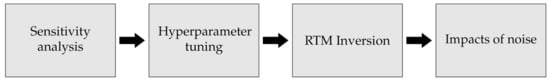
Figure 1.
The first step consists of identifying which biophysical variables can be detected by S2 while the second step uses Bayesian optimization to find the best parameters for the various models. Lastly, the third and fourth steps test the performance of the various algorithms for inverting simulated S2-like data using Radiative Transfer Models in pure and noisy conditions.
The third part consists of testing the ability of the most commonly used algorithms for RTM inversion: Random Forests [34], Artificial Neural Networks [35], and Gaussian Processes [36]. Each of is representative of the different families of algorithms commonly used for RTM inversion [26]. The final step consists of evaluating the resilience of the above models to increasing levels of noise. Before describing each of the steps in more detail, we first describe the selected RTM, i.e., PROSAIL, [37], and the selected algorithms for RTM inversion.
2.2. PROSAIL
PROSAIL is the most common RTM used for biophysical trait retrievals, and the most used in Hybrid approaches. PROSAIL is actually the coupling of two core models: PROSPECT [38,39,40] and SAIL [37]. PROSPECT uses well-established physical principles of light-matter interaction to simulate how light interacts with a single leaf. SAIL stands for Scattering by Arbitrarily Inclined Leaves and is based on the plate model initially proposed by Suits [41]. The basic principle of SAIL is that vegetation canopy can be represented by a “plate” that interacts with directional incoming radiation. PROSAIL integrates both models by characterizing the vegetation canopy using SAIL and the leaves by using PROSPECT [42]. The result of the model is a description of the reflectance of the vegetation layer as dependent on the relative positions of the sun, sensor, canopy and soil characteristics. The ranges of parameters used for this research are described in Table 1 and were intentionally broader than what is commonly found in other publications (e.g., [42]) to ensure the full range of possible values of these parameters [43].

Table 1.
Overview of PROSAIL input parameters used. Trait combinations were sampled representatively using a Latin hypercube sampling approach across the range identified. For the ML sections, was fixed at 10.
2.3. Machine Learning Algorithms
2.3.1. Random Forest
The Random Forest regression (RFR) [34] is a type of ensemble classifier that combines multiple Classification and regression Trees (CART) through bagging and boosting. In each iteration, RFR bins the data to different sets and maximizes the “purity” of each through a given purity index (e.g., Gini index). To formalize the procedure, let s be a candidate split value at a given node t, then the decrease in impurity is given by:
where and are the proportion of data for each node, is the node impurity before splitting and and are the measures of impurity after splitting. While in CART, a single decision tree () is used, in RFR multiple (K) are trained and fitted to a set of data x, and the final prediction results from either a majority (classification) or the mean (regression). Formalizing, RFR is an ensemble of K decision trees , fitted to a set of data x:
Furthermore, RFR uses the bootstrap aggregating technique to reduce the correlation between trees and increases the accuracy and stability of the final model [34]. An advantage of RFR is its ability to provide an estimate of prediction error without the need for external data since, in each iteration, data non-contributing for model construction is used for internal testing (out-of-bag error, obb) and to control model overfitting [34].
2.3.2. Artificial Neural Networks
Artificial Neural Networks (ANN) were initially proposed as a computational model for learning inspired by the biological brain [35]. ANN have since been extensively used in numerous applications due to their particular ability to model non-linear and complex relationships, and to provide accurate predictions even on unseen data [44]. Two other important characteristics of neural networks are that they allow the user to adapt the architecture to the task itself, and that they are fully data-driven approaches that impose no limitations on the distribution of input data [44,45]. ANN are often represented as graphs where each node is a neuron and is interconnected with other neurons appearing similar to a biological brain. Each neuron in an ANN consists of a mapping function:
where w, b represent the weight and bias of each ith neuron, and x, y represent the input and output of the hidden layer. Furthermore, the output y of each neuron can also be plugged into a function, known as activation functions, which can be used to enforce a specific behavior to each neuron/layer. Each set of interconnected layers of neurons, except for the input and output sets, are known as hidden layers. The procedure for training a supervised ANN consists of minimizing the difference of the current model prediction against the desired outcome by propagating small changes in w and b of all neurons on all layers in each iteration (epoch).
For this research, we used two different neural networks: a densely connected and feed-forward ANN with back-propagation training. This is one of the most used architectures and is used also by the ESA SNAP toolbox [46]. The second architecture is a feed-forward, Multi-task Neural Network (MTN) with back-propagation training. This second type of architecture is increasingly more common thanks to the possibility of partitioning the learning tasks [45].
2.3.3. Gaussian Processes
Gaussian Process Regression (GPR) [36], also known as kriging, is a type of non-parametric regression modeling. GPR relies on the Bayes method for inference and a pre-set covariance kernel function that is optimized to fit the given data. A Gaussian Process is defined as , is a set of random variables with a Gaussian distribution that is normally distributed in the multivariate space. Under these conditions, there exists a mean () of the multivariate distribution, a covariance function (k) that represents the covariance between each point and an expected level of Gaussian noise with standard deviation :
where x represents sets of observed points, and k a prior covariance function enforced for designing the covariance matrix. represents noise being added along the diagonal of the covariance function. This formulation implies that is a linear combination of underlying sets of Gaussian Processes and predictions on any given location are interpolations of the observed data. The covariance functions are known as kernels and provide the expected correlation between different observations. The kernel functions tested in this research were: radial basis function (RBF), rational Quadratic, matérn, and the dot product.
The main benefits of GPR lie in its versatility [47] and the ability to produce good results even with a limited number of training data [20]. Furthermore, GPR can provide an empirical estimate of the uncertainty of the prediction given the evidence x and the joint distribution defined by the covariance matrix k. The caveat is that they are computationally expensive when using a large data set [15], and that the model requires storing the entire covariance matrix information which increases the memory load as the covariance matrix grows quadratically () as a function of n data points.
2.4. Step 1: Sensitivity Analysis
We explored which biophysical variables can be estimated by S2. We considered only the most significant leaf and canopy traits of , , , and and analysed them through two different approaches: the first explores the correlations between any S2 band and a given trait using Spearman’s rank correlation coefficient (). For this, 100 uniformly distributed random samples of traits were generated, and its canopy spectral response was obtained using PROSAIL and convoluted into S2 bands. Then, the Spearman’s correlation between each trait and band was calculated. This analysis quantifies the association between pairs of bands and biophysical variables and is indicative of the overlap in correlations between different variables. However, it does not provide any further inference relative to combined effects, or a breakdown in direct and indirect interactions, that variations in biophysical variables can have on the various S2 bands.
The second approach explores the sensitivity of S2 data to variation in biophysical variables using a GSA index. The GSA was used to quantify the actual sensitivity of each band to each trait as well as the interactions between bands. This analysis was performed by using EFAST [31] which is a variance-based global sensitivity analysis that combines Fourier transformations with Sobol’s method to decompose the various effects [48]. These effects are decomposed into first-order, interaction and total-order sensitivity indices that represent the variability associated with single features, interactions between features, and the sum of all interactions, respectively. This allowed us to explore which S2 bands are associated with which biophysical trait and if there are significant confounding factors between them, and is an analysis comparable to what was performed by Gu et al. [49] and Brede et al. [27]. Since the EFAST provides an estimate of the sensitivity, a conservative number of samples necessary to provide an accurate estimate must be identified first by calculating the index with increasing number of samples until the estimate stabilizes.
2.5. Step 2: Hyperparameter Tuning
A critical first step in any ML is hyperparameter tuning. This step thus consists of identifying the best combination of the ML model hyperparameters for the task of RTM inversion. As mentioned in Section 2.3, each of the aforementioned algorithms have different sets of parameters that should be tuned. Therefore, hyperparameter tuning is particularly important when comparing such different ML algorithms to ensure fairness. Thus, and in contrast to [50], Bayesian optimization was applied for hyperparameter optimization instead of on the RTM inversion itself (Step 3). Table 2 shows the range of hyperparameters used for this procedure.
Table 2.
Overview of the hyperparameters tested during the optimization. The final set of parameters used are given in Tables 4 and 5.
The hyperparameter tuning task was performed using the TPE approach with the hyperopt package in Python [32]. This method consists of a sequential optimization procedure that uses Bayesian inferences to explore the potential solution space and identify the best combination of hyperparameters. This procedure was performed using 1800 samples with a 10-k fold cross-validation evaluation of the training error and 200 sequential evaluations of the parameters. Once the hyperparameters for the models were selected, we identified the number of training epochs for the ANN. We tested this by analysing the effect of the number of epochs on the prediction error and concluded that 500 epochs was reasonable number between the over-fitting risk and training time (see Figure A1).
2.6. Step 3: RTM Inversion
The inversion of RTM data followed a hybrid approach, as proposed by Verrelst et al. [26]. Trait data was generated using a Latin hypercube sampling approach based on the trait space and parameters as shown in Table 1. The data generated with PROSAIL represents the canopy reflectance from 400 to 2500 nm with a resolution of 1 nm. However, the S2 data only measure reflectance in specific bands. Therefore, to convert the PROSAIL data to S2 resolution, we used a weighted sum spectral convolution approach:
where for each independent band, the weights (w) were obtained from the spectral responses provided by ESA for S2A [51], and the represents the reflectance values obtained from PROSAIL for each band at wavelength i. Finally, only the band products provided at 10–20 m in the final level 2A product were used: i.e., bands 2, 3, 4, 5, 6, 7, 8A, 11 and 12.
To evaluate the performance of the models, we opted to use the Mean Absolute Percentage Error (MAPE) because it provides an intuitive interpretation and is easily comparable between all traits. This is important for this case since the different biophysical variables have very different ranges of values (see Table 1), and this way we ensure a proper and intuitive interpretation of the results across the board. MAPE is calculated by:
where and are the reference and predicted data, respectively, and n the number of data points used for validation. In the absence of noise, the next step was to partition the data into the three sets needed for cross-validation: of the total data was left out for estimating the validation error; the remaining of the total data was used for both the algorithm training and to estimate the training error through a 10 k-fold leave-one-out approach. All tested algorithms were trained under identical conditions and using the same training data in each run. To identify how many samples are needed for inverting PROSAIL RTM, we incremented from a minimum of 50 samples to 4000 samples by steps of 250. This experiment allowed us to identify both the best algorithm for PROSAIL RTM inversion as well as their data needs.
2.7. Impacts of Noise
To assess the impact of noise on the accuracy of each model, we explored how increasing levels of correlated Gaussian noise affected the accuracy of the models as shown in Figure 2. Two noise models were tested, as defined by Locherer et al [25]:
where , represent the noisy signal and pure simulated spectra, and the wavelength. While both models add noise as a function of wavelength, the Inverted model will affect more bands on the visible and SWIR regions of the spectra, while the Combined model will affect more the IR region. Using both types of Gaussian models, we tested the effect of the following increasing levels of noise added to the training data: 1%, 3%, 5%, 10%, 15%, 20%, 25%, 30%, 40%, and 50%. This experiment aims to explore the pervasiveness of noisy data in the performance of the ML RTM inversion.
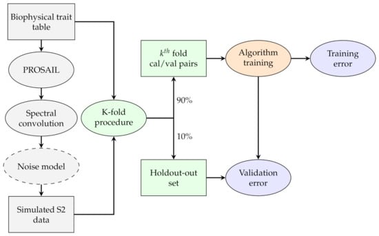
Figure 2.
Flowchart representing the training and validating procedure of the experiments. All algorithms were trained with the same data to exclude any random effect. The noise is only added in the second part of the experiment when testing its effect on the error.
3. Results
3.1. Sensitivity Analysis
The Spearman rank correlation coefficients are shown in Table 3, while the scatterplots are shown in Figure 3. Many significant were found between multiple pairs of bands and traits. These relationships are, however, not linear as seen in Figure 3. was shown to have a negative correlation with all visible bands and had a negligible correlation with the remaining biophysical parameters (Table 3). Somewhat inversely, is strongly negatively correlated with the two bands in the longest wavelengths (B11 and B12). and are both strongly correlated with the NIR and SWIR bands, while has a positive correlation (Table 3). It is also seen that has a negative correlation, indicating a high potential for interaction in these bands (Table 3). Finally, is only significantly correlated with the blue band. was found to be almost exclusively associated with B11 and B12, which indicates that there might be also some degree of correlation between and (Figure 3 and Table 3).
Table 3.
Summary of Spearman’s correlation coefficients for different biophysical variables and S2 bands. The significance levels are represented as: (***); (**); (*); (.); : no symbol.
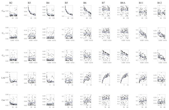
Figure 3.
Scatterplot between each trait and band. To improve visualization, only a fraction of 100 samples were used in this plot.
We found that for around 2000 samples the variation on the estimate of GSA stabilized; therefore, we used this number of samples to analyse the sensitivity (Figure 4). The final GSA estimates (Figure 5) show that was most associated with the three bands on the red-edge region B6, B7 and B8A, and most of the sensitivity on each band was of first-order. was strongly dependent on bands B11 and B12, with some interaction effects occurring on B12. was shown to be sensitive to variations in multiple bands from the infrared region (B06, B07 and B8A) to the short-wave infrared region (B11 and B12). Some interaction between and can be observed in B12. was found to be exclusively dependent on the blue band (B2), which is of concern due to the high degree of interaction with . This, combined with the lack of variation in reflectance (see Figure A2), indicates that cannot be detected by S2 data simulated by PROSAIL; therefore, we excluded it from the remainder of the analysis.
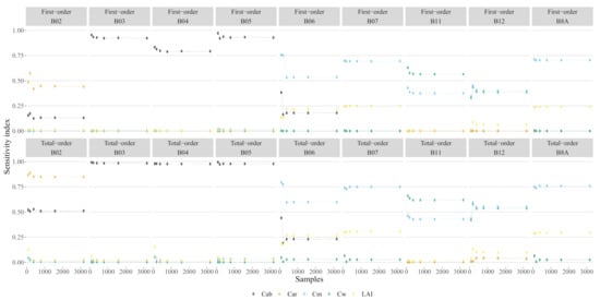
Figure 4.
Global sensitivity index EFAST as function of the number of samples.
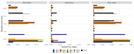
Figure 5.
The sensitivity index as a function of each trait. The first-order sensitivity is the sensitivity associated with each trait while the total order is the sum of the first order with the interactions.
3.2. Hyperparameter Tuning
The final hyperparameter obtained for each model are shown in Table 4 and Table 5. While the first shows the overall parameters for the RFR, GPR, and both ANN, the second shows the task-specific parameters for the MTN. For the RFR, 850 trees were selected with a negligible minimum number of sample being used for node or leaf splitting. For GPR, it was found that 80 optimization procedures were necessary, using a rational quadratic kernel.
Table 4.
Summary of selected hyperparameters. * on the multi-task network are related to the shared layers; task-specific parameters are given in Table 5.
Table 5.
Summary of selected hyperparameters for the trait-specific layers
In the case of the neural networks, for all cases, the maximum number of hidden layers was selected and with a high number of neurons (Table 4 and Table 5). Non-linear activation functions were selected with different functions for the ANN and MTN (shared layers). For the MTN, less complexity was found on the layers associated with and , while more complexity was needed for , and especially for , as shown by the need for more neurons in each hidden layer (Table 4 and Table 5). This is of particular interest since it is well established that reflectance often saturates at higher levels of (Table 4 and Table 5).
3.3. RTM Inversion
When inverting PROSAIL spectra without any added noise (Figure 6 and Figure 7, see Table 4 and Table 5 for details), the RFR was overall the worst performing model by converging on and at approximately 45% and 50% MAPE. Only for did RFR approximate the performance of the other models. The worst performance of ANN was in estimation where MAPE converged at 5%, while on all other variables it achieved a MAPE of approximately 2%. The MTN converged faster and showed a significant improvement in accuracy in all biophysical variables by achieving approximately 2% error in all target traits. GPR was by far the best performing model with a negligible MAPE in all biophysical variables, even with fewer than 1000 samples.
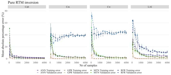
Figure 6.
Model performance on pure PROSAIL RTM simulation. While each model has its own color, the darker colors represent the training error. The data used for these plots is accessible in the Github repository provided at the end of this manuscript.
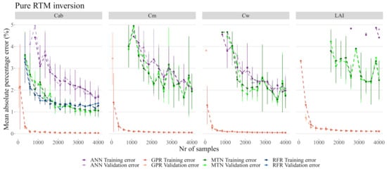
Figure 7.
Detail of Figure 6 between 0 and 5%.
While most models produced errors below 2.5% on , the RFR was the worst overall model by being unable to properly predict or , and not being able to predict with less than 10% error (Figure 7). The GSA analysis showed that these three biophysical variables are likely correlated and interacting (see Table 3 and Figure 5) and thus RFR was not able to address this effect. MTN outperformed ANN both in terms of the MAPE error as well as in terms of the number of samples necessary for accurate predictions. Although the actual MAPE error is small for both ANN and MTN, it was also several orders of magnitude larger than the MAPE error of GPR. For the remainder of the analysis, 2000 samples were used given that the error margins did not improve significantly with a larger sample size (Figure 7).
3.4. Impacts of Noise
Adding noise to the models had a noticeable impact on the model performance, with all of them showing quick and significant degradation of performance. In particular, GPR was no longer the best performing model for the entire range of noise levels tested, and instead, MTN showed slightly better results (Figure 8). Increasing noise levels resulted in saturation of the prediction error for all traits, with getting the highest MAPE error. Interestingly, for and , the RFR error rate did not change significantly and all models eventually converged to the same error level.
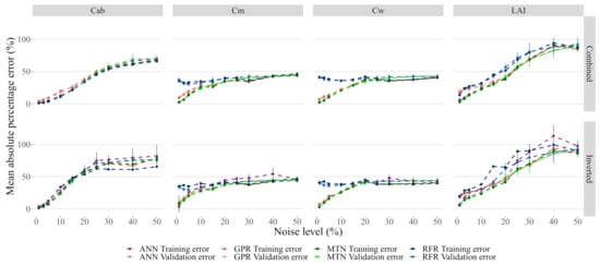
Figure 8.
Effect of noise on model performance. While each model has its own color, the darker colors represent the training error. The data used for these plots is accessible in the Github repository provided at the end of this manuscript.
Inverted noise affected the prediction accuracy more than Combined noise. This effect is particularly evident for , and , even at low levels of noise (Figure 9). For low values of added noise, the neural networks were the best performing model for most traits/noise models, even if the absolute error increased significantly. Furthermore, MTN performed better than ANN and showed more resilience to noise.
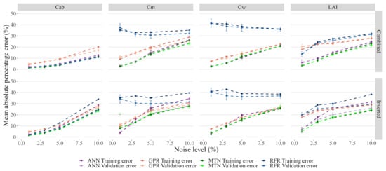
Figure 9.
Detail of Figure 8 between 0 and 10% added noise.
4. Discussion
The results of our sensitivity analysis provided clear insights into which biophysical variables can be measured using S2 data (see Figure 5 and Table 3), and furthermore, provided insights into the effects of their interaction with spectral responses. Our results on the band correlation (Table 3) and sensitivity analysis (Figure 5) are in line with previous results [52], and in particular, when compared with recent results by Brede et al. [27] also on S2 data, and Gu et al. [49] on Landsat TM data. Similarly, both studies found that was associated with the visible range in Landsat TM bands, and that , and was associated with NIR and SWIR bands (see Figure 5). The GSA analysis also shows that , and have a degree of interaction between, them which has also been experienced in previous research [15,52,53]. These interactions can have serious implications for the accuracy of the retrievals, as specific traits can be more easily inverted due to a higher number of dedicated bands (e.g., ), while others are more vulnerable to interactions (e.g., and ). On top of that, from a biological perspective, it is also likely that some traits vary together (e.g., and ). The main difference for S2 is on which bands are sensitive to which biophysical variables: in our case, the red-edge (5 and 6) and NIR (8A) were most strongly associated with , which can be indicative of this sensor being more suited for estimates but also possessing a higher potential for correlations and interactions. A significant output of this analysis is that is hardly measurable by S2 because only band B2 showed sensitivity with a high degree of interaction with (Figure 5), and almost no variation is detectable (see Figure A2).
The use of the Tree-structured Parzen Estimator showed that deeper and more complex architectures yield better results. This is notable when comparing the ANN with MTN and observing that a different number of neurons and activation functions were selected as a function of the objective trait (see Table 4 and Table 5). In the case of MTN, and consistent with sensitivity analysis (Figure 5), more complex architectures were selected by the optimization procedure for the traits with higher degrees of interactions (see Figure 5 and Table 5). This is also in line with other results in other fields of ML where it has been shown that automatic procedures can greatly improve the model performance and infer specific domain knowledge [49]. Together, these results can have significant implications for the commonly used architectures, which are often simpler (e.g., ESA SNAP) and suggest that more complex architectures can improve the retrieval of biophysical variables. Furthermore, encoding hyperparameter tuning approaches into retrieval procedures can increase the model versatility by adapting it to specific location or trait-spaces. In addition, although these adaptations would be hindered by the high computational cost of hyperparameter tuning [54], recent developments in the field of AutoML are addressing this through the concept of meta-learning [55] and multi-layer stacking [56] which minimize the computational costs for finding suitable models.
Not all ML algorithms were found to be equally capable of hybrid inversion of pure S2 data (Figure 6 and Figure 7). As with most recent research, [10,20,57] found the Gaussian Processes produced the best results for pure signals by significant levels of magnitude. This is of particular importance when considering that the use of Gaussian Processes for this task is less common than the use of other methods such as ANN [15] or RFR [17]. While in our case, we found that RFR is unfit for hybrid inversion of S2 data, Campos-Taberner et al. [19] successfully mapped biophysical variables using this algorithm on MODIS data, implying that these results are dependent also on the sensors used - and intersecting with the concept of meta-learning [55], model pipelines trained on sensors with different bands can potentially provide pre-set model hyperparameters that are transferable between sensors.
Model performance was severely affected even at low levels of noise (Figure 8 and Figure 9). This is of particular concern given that every data has noise, and previous research has shown that the Sen2Cor atmospheric correction algorithm produces between 5% and 10% noise [27,52]. Moreover, and in contrast to results obtained on pure data, both neural networks generally performed better than GPR when noise was added, which indicates that further developments with GPR are needed to be able to deal effectively with noisy observations. Recently, Svendsen et al. [58] showed how GPR can be extended to more complex, structures similar deep learning neural networks and is worth exploring in future research.
As expected, noise did not affect all bands equally [52], which is consistent with the different band selection and interactions according to the sensitivity analysis (see Figure 5). In line with this, estimates were shown to be more resilient to noise, which can be explained by the high number of bands associated with this trait as well as their lack of interaction. The opposite was observed for , and , which share many of the same band sensitivities and behaved similarly when noise was added. Nevertheless, the error dependence on each trait implies that specific care to each trait should be given when using a hybrid approach for RTM inversion in S2. Two potential approaches to minimize the trait specific error are (1) to encode more hyperparameter optimization effort towards inverting the more vulnerable traits (2) to when using neural networks, enforce task-sharing and task specific layers on these known interactions.
For practical purposes, in the case of global predictions of biophysical variables, both GPR and the two neural networks (ANN and MTN) have specific advantages and disadvantages. For example, ANN are models that can be continuously updated without significant increases in terms memory requirements as new training implies only changing the weights and biases of the neurons and hidden layers. This implies that it is trivial to share pre-trained neural networks for the entire globe which can be used as meta-learning models for warm-starting the hyperparameter tuning optimization procedures tailored for each location/sensor. On the other hand, GPR requires a very low number of samples to stabilize its prediction and offers Active Learning opportunities that combine field measurements with hybrid inversion within the model itself [20,59]. The caveats regarding GPR are its tendency to overfit if given too much data, its training time scaling cubically in function of the number samples [47,60], thus increasing its computational load and cost. Another important aspect regarding GPR is that optimizing this model for tasks implies either prior knowledge to impose a specific behaviour to the model or complex methods for structure discovery due to the additive and multiplicative properties of the kernels [47]. A possible solution to address these challenges which has not yet been fully explored could be to combine Decision Trees or Random Forests with Gaussian Processes [60], by clustering the data into similar groups and applying GPR on the leaf nodes.
A final concern is that most approaches for hybrid inversion work on the assumption that there are no known correlations between the biophysical variables. In nature, it is virtually impossible to observe random combinations of traits as were used for model training, e.g., a leaf with of 10 but no . The lack of real-world correlations between biophysical variables likely aggravates the ill-posedness problem and future research on exploring approaches that can include known correlations between biophysical variables or exclude unrealistic combinations will likely contribute to improvements without necessarily losing generalization [61].
Further potential avenues for improving the retrieval of biophysical parameters using RTM inversion include the ingestion of a priori knowledge of the ecosystem and trait-space understudy. Such ancillary information can help reduce the range of input parameters used which in turn limits the solution space and related degree of ill-posedness [62]. In dealing with ill-posedness, Rivera et al., 2013 [63] has suggested the use of an ensemble approach which could prove helpful in reducing uncertainties in real-world applications. Band selection methods and the use of spectral indices (ratio) in addition to spectral bands to train inversion models can be also be explored as earlier results have shown [10,64].
In many cases, RTMs are used as surrogate information given the lack of field data due to these campaigns being particularly labour intensive and costly. If more data were available, more data-driven approaches could be implemented, and the requirement of RTM-based inversions can be minimized. While plant trait database conglomerates such as TRY [43] or continental-scale observatory networks such as NEON [65] are a vital step in the right direction, further steps are needed to make use of the unprecedented availability of EO data and cloud computing solutions that are increasingly available for researchers.
5. Conclusions
This study shows that biophysical variables can be obtained successfully from S2 data using a hybrid inversion of PROSAIL RTM. Within such inversion, Gaussian Processes outperform all other models when using pure data. However, with added noise, this is no longer true, and ANN, MTN, and GPR have similar results, with the neural networks being slightly better. Moreover, while GPR can be trained quicker and with less data, neural network architectures offer a lot of opportunities for improvement and less computational load. Therefore, more complex neural network architectures should be explored to improve the accuracy and generality of biophysical trait retrieval on global scale. Such future explorations may also benefit from the integration of ecological knowledge into the training procedure, e.g., by imposing these relationships on the training data itself and from automatic hyperparameter tuning based on sensor, location, and objects. Other future opportunities can arise with the increasing number of publicly available trait databases and sensors which can allow the development of meta-learning approaches that could improve both the model performance as well as reduce the computational cost. In combination, this study provides a major encouragement for using hybrid RTM inversion to retrieve biophysical variables from satellite data, e.g., for monitoring global change impacts.
Author Contributions
N.C.d.S. was responsible for the conceptualization, implementation, execution and preparation of this manuscript. M.B. was responsible for the conceptualization, assisted in the implementation and contributed for the preparation of this manuscript. L.T.H. contributed for the conceptualization and preparation of the manuscript. P.v.B. contributed for the conceptualization and preparation of the manuscript. All authors have read and agreed to the published version of the manuscript.
Funding
This research was partly funded through the Leiden University Data Science Research Program.
Code Availability
https://github.com/nunocesarsa/RTM_Inversion (accessed on 2 December 2020).
Acknowledgments
The authors would like to acknowledge the three reviewers for their valuable comments and suggestions that greatly improved the manuscript. The authors would also like to acknowledge Andrew Sorensen for his review of the English quality of this manuscript.
Conflicts of Interest
The authors declare no conflict of interest.
Appendix A
Appendix A.1. Spectral Variability in Response to Trait Variability

Figure A1.
Neural networks training and validation error in function of epochs. Error bars represent the standard deviation of a 5-fold cross-validation procedure.
Figure A1.
Neural networks training and validation error in function of epochs. Error bars represent the standard deviation of a 5-fold cross-validation procedure.

Appendix A.2. Artificial Neural Networks Mean Absolute Percentage Error in Function of Training Epochs

Figure A2.
With this figure it is possible to visualize the variation in PROSAIL simulated S2-like data reflectance spectra when stabilizing all traits except for one. This shows that variations in Car are likely not measurable by Sentinel-2.
Figure A2.
With this figure it is possible to visualize the variation in PROSAIL simulated S2-like data reflectance spectra when stabilizing all traits except for one. This shows that variations in Car are likely not measurable by Sentinel-2.

References
- Pereira, H.M.; Ferrier, S.; Walters, M.; Geller, G.N.; Jongman, R.H.G.; Scholes, R.J.; Bruford, M.W.; Brummitt, N.; Butchart, S.H.M.; Cardoso, A.C.; et al. Essential Biodiversity Variables. Science 2013, 339, 277–278. [Google Scholar] [CrossRef] [PubMed]
- Jetz, W.; McGeoch, M.A.; Guralnick, R.; Ferrier, S.; Beck, J.; Costello, M.J.; Fernandez, M.; Geller, G.N.; Keil, P.; Merow, C.; et al. Essential biodiversity variables for mapping and monitoring species populations. Nat. Ecol. Evol. 2019, 3, 539–551. [Google Scholar] [CrossRef] [PubMed]
- Vihervaara, P.; Auvinen, A.P.; Mononen, L.; Törmä, M.; Ahlroth, P.; Anttila, S.; Böttcher, K.; Forsius, M.; Heino, J.; Heliölä, J.; et al. How Essential Biodiversity Variables and remote sensing can help national biodiversity monitoring. Glob. Ecol. Conserv. 2017, 10, 43–59. [Google Scholar] [CrossRef]
- Pettorelli, N.; Schulte to Bühne, H.; Tulloch, A.; Dubois, G.; Macinnis-Ng, C.; Queirós, A.M.; Keith, D.A.; Wegmann, M.; Schrodt, F.; Stellmes, M.; et al. Satellite remote sensing of ecosystem functions: Opportunities, challenges and way forward. Remote Sens. Ecol. Conserv. 2017, 4, 71–93. [Google Scholar] [CrossRef]
- Cavender-Bares, J.; Gamon, J.A.; Townsend, P.A. (Eds.) Remote Sensing of Plant Biodiversity; Springer: Berlin/Heidelberg, Germany, 2020. [Google Scholar] [CrossRef]
- Ghamisi, P.; Gloaguen, R.; Atkinson, P.M.; Benediktsson, J.A.; Rasti, B.; Yokoya, N.; Wang, Q.; Hofle, B.; Bruzzone, L.; Bovolo, F.; et al. Multisource and Multitemporal Data Fusion in Remote Sensing: A Comprehensive Review of the State of the Art. IEEE Geosci. Remote Sens. Mag. 2019, 7, 6–39. [Google Scholar] [CrossRef]
- Nock, C.A.; Vogt, R.J.; Beisner, B.E. Functional Traits. eLS 2016. [Google Scholar] [CrossRef]
- Asner, G.P. Biophysical and Biochemical Sources of Variability in Canopy Reflectance. Remote Sens. Environ. 1998, 64, 234–253. [Google Scholar] [CrossRef]
- Weiss, M.; Baret, F.; Myneni, R.B.; Pragnère, A.; Knyazikhin, Y. Investigation of a model inversion technique to estimate canopy biophysical variables from spectral and directional reflectance data. Agronomie 2000, 20, 3–22. [Google Scholar] [CrossRef]
- Verrelst, J.; Dethier, S.; Rivera, J.P.; Munoz-Mari, J.; Camps-Valls, G.; Moreno, J. Active Learning Methods for Efficient Hybrid Biophysical Variable Retrieval. IEEE Geosci. Remote Sens. Lett. 2016, 13, 1012–1016. [Google Scholar] [CrossRef]
- Durán, S.M.; Martin, R.E.; Díaz, S.; Maitner, B.S.; Malhi, Y.; Salinas, N.; Shenkin, A.; Silman, M.R.; Wieczynski, D.J.; Asner, G.P.; et al. Informing trait-based ecology by assessing remotely sensed functional diversity across a broad tropical temperature gradient. Sci. Adv. 2019, 5, eaaw8114. [Google Scholar] [CrossRef]
- Schneider, F.D.; Morsdorf, F.; Schmid, B.; Petchey, O.L.; Hueni, A.; Schimel, D.S.; Schaepman, M.E. Mapping functional diversity from remotely sensed morphological and physiological forest traits. Nat. Commun. 2017, 8. [Google Scholar] [CrossRef] [PubMed]
- Zarco-Tejada, P.; Hornero, A.; Beck, P.; Kattenborn, T.; Kempeneers, P.; Hernández-Clemente, R. Chlorophyll content estimation in an open-canopy conifer forest with Sentinel-2A and hyperspectral imagery in the context of forest decline. Remote Sens. Environ. 2019, 223, 320–335. [Google Scholar] [CrossRef] [PubMed]
- Verrelst, J.; Camps-Valls, G.; Muñoz-Marí, J.; Rivera, J.P.; Veroustraete, F.; Clevers, J.G.; Moreno, J. Optical remote sensing and the retrieval of terrestrial vegetation bio-geophysical properties—A review. ISPRS J. Photogramm. Remote Sens. 2015, 108, 273–290. [Google Scholar] [CrossRef]
- Verrelst, J.; Malenovský, Z.; der Tol, C.V.; Camps-Valls, G.; Gastellu-Etchegorry, J.P.; Lewis, P.; North, P.; Moreno, J. Quantifying Vegetation Biophysical Variables from Imaging Spectroscopy Data: A Review on Retrieval Methods. Surv. Geophys. 2018, 40, 589–629. [Google Scholar] [CrossRef]
- Staben, G.; Lucieer, A.; Scarth, P. Modelling LiDAR derived tree canopy height from Landsat TM, ETM+ and OLI satellite imagery—A machine learning approach. Int. J. Appl. Earth Obs. Geoinf. 2018, 73, 666–681. [Google Scholar] [CrossRef]
- Moreno-Martínez, Á.; Camps-Valls, G.; Kattge, J.; Robinson, N.; Reichstein, M.; van Bodegom, P.; Kramer, K.; Cornelissen, J.H.C.; Reich, P.; Bahn, M.; et al. A methodology to derive global maps of leaf traits using remote sensing and climate data. Remote Sens. Environ. 2018, 218, 69–88. [Google Scholar] [CrossRef]
- Darvishzadeh, R.; Wang, T.; Skidmore, A.; Vrieling, A.; O’Connor, B.; Gara, T.; Ens, B.; Paganini, M. Analysis of Sentinel-2 and RapidEye for Retrieval of Leaf Area Index in a Saltmarsh Using a Radiative Transfer Model. Remote Sens. 2019, 11, 671. [Google Scholar] [CrossRef]
- Campos-Taberner, M.; Moreno-Martínez, Á.; García-Haro, F.; Camps-Valls, G.; Robinson, N.; Kattge, J.; Running, S. Global Estimation of Biophysical Variables from Google Earth Engine Platform. Remote Sens. 2018, 10, 1167. [Google Scholar] [CrossRef]
- Svendsen, D.H.; Martino, L.; Campos-Taberner, M.; Camps-Valls, G. Joint Gaussian processes for inverse modeling. In Proceedings of the 2017 IEEE International Geoscience and Remote Sensing Symposium (IGARSS), Fort Worth, TX, USA, 4 December 2017. [Google Scholar] [CrossRef]
- Camps-Valls, G.; Martino, L.; Svendsen, D.H.; Campos-Taberner, M.; Muñoz-Marí, J.; Laparra, V.; Luengo, D.; García-Haro, F.J. Physics-aware Gaussian processes in remote sensing. Appl. Soft Comput. 2018, 68, 69–82. [Google Scholar] [CrossRef]
- Tuia, D.; Verrelst, J.; Alonso, L.; Perez-Cruz, F.; Camps-Valls, G. Multioutput Support Vector Regression for Remote Sensing Biophysical Parameter Estimation. IEEE Geosci. Remote Sens. Lett. 2011, 8, 804–808. [Google Scholar] [CrossRef]
- Annala, L.; Honkavaara, E.; Tuominen, S.; Pölönen, I. Chlorophyll Concentration Retrieval by Training Convolutional Neural Network for Stochastic Model of Leaf Optical Properties (SLOP) Inversion. Remote Sens. 2020, 12, 283. [Google Scholar] [CrossRef]
- Zurita-Milla, R.; Laurent, V.; van Gijsel, J. Visualizing the ill-posedness of the inversion of a canopy radiative transfer model: A case study for Sentinel-2. Int. J. Appl. Earth Obs. Geoinf. 2015, 43, 7–18. [Google Scholar] [CrossRef]
- Locherer, M.; Hank, T.; Danner, M.; Mauser, W. Retrieval of Seasonal Leaf Area Index from Simulated EnMAP Data through Optimized LUT-Based Inversion of the PROSAIL Model. Remote Sens. 2015, 7, 10321–10346. [Google Scholar] [CrossRef]
- Verrelst, J.; Rivera, J.P.; Veroustraete, F.; Muñoz-Marí, J.; Clevers, J.G.; Camps-Valls, G.; Moreno, J. Experimental Sentinel-2 LAI estimation using parametric, non-parametric and physical retrieval methods—A comparison. ISPRS J. Photogramm. Remote Sens. 2015, 108, 260–272. [Google Scholar] [CrossRef]
- Brede, B.; Verrelst, J.; Gastellu-Etchegorry, J.P.; Clevers, J.G.P.W.; Goudzwaard, L.; den Ouden, J.; Verbesselt, J.; Herold, M. Assessment of Workflow Feature Selection on Forest LAI Prediction with Sentinel-2A MSI, Landsat 7 ETM+ and Landsat 8 OLI. Remote Sens. 2020, 12, 915. [Google Scholar] [CrossRef]
- Berger, K.; Caicedo, J.P.R.; Martino, L.; Wocher, M.; Hank, T.; Verrelst, J. A Survey of Active Learning for Quantifying Vegetation Traits from Terrestrial Earth Observation Data. Remote Sens. 2021, 13, 287. [Google Scholar] [CrossRef]
- Upreti, D.; Huang, W.; Kong, W.; Pascucci, S.; Pignatti, S.; Zhou, X.; Ye, H.; Casa, R. A Comparison of Hybrid Machine Learning Algorithms for the Retrieval of Wheat Biophysical Variables from Sentinel-2. Remote Sens. 2019, 11, 481. [Google Scholar] [CrossRef]
- Xie, Q.; Dash, J.; Huete, A.; Jiang, A.; Yin, G.; Ding, Y.; Peng, D.; Hall, C.C.; Brown, L.; Shi, Y.; et al. Retrieval of crop biophysical parameters from Sentinel-2 remote sensing imagery. Int. J. Appl. Earth Obs. Geoinf. 2019, 80, 187–195. [Google Scholar] [CrossRef]
- Saltelli, A.; Tarantola, S.; Chan, K.P.S. A Quantitative Model-Independent Method for Global Sensitivity Analysis of Model Output. Technometrics 1999, 41, 39–56. [Google Scholar] [CrossRef]
- Bergstra, J.; Yamins, D.; Cox, D.D. Making a Science of Model Search: Hyperparameter Optimization in Hundreds of Dimensions for Vision Architectures. In Proceedings of the 30th International Conference, International Conference on Machine Learning, Atlanta, GA, USA, 17–19 June 2013; pp. I-115–I-123. [Google Scholar]
- Bergstra, J.; Komer, B.; Eliasmith, C.; Yamins, D.; Cox, D.D. Hyperopt: A Python library for model selection and hyperparameter optimization. Comput. Sci. Discov. 2015, 8, 014008. [Google Scholar] [CrossRef]
- Breiman, L. Random Forests. Mach. Learn. 2001, 45, 5–32. [Google Scholar] [CrossRef]
- McCulloch, W.S.; Pitts, W. A logical calculus of the ideas immanent in nervous activity. Bull. Math. Biophys. 1943, 5, 115–133. [Google Scholar] [CrossRef]
- Rasmussen, C.E.; Williams, C.K.I. Gaussian Processes for Machine Learning (Adaptive Computation and Machine Learning); The MIT Press: Cambridge, MA, USA, 2005. [Google Scholar]
- Verhoef, W. Light scattering by leaf layers with application to canopy reflectance modeling: The SAIL model. Remote Sens. Environ. 1984, 16, 125–141. [Google Scholar] [CrossRef]
- Jacquemoud, S.; Baret, F. PROSPECT: A model of leaf optical properties spectra. Remote Sens. Environ. 1990, 34, 75–91. [Google Scholar] [CrossRef]
- Jacquemoud, S.; Verhoef, W.; Baret, F.; Bacour, C.; Zarco-Tejada, P.J.; Asner, G.P.; François, C.; Ustin, S.L. PROSPECT + SAIL models: A review of use for vegetation characterization. Remote Sens. Environ. 2009, 113, S56–S66. [Google Scholar] [CrossRef]
- Féret, J.B.; Gitelson, A.; Noble, S.; Jacquemoud, S. PROSPECT-D: Towards modeling leaf optical properties through a complete lifecycle. Remote Sens. Environ. 2017, 193, 204–215. [Google Scholar] [CrossRef]
- SUITS, G. The calculation of the directional reflectance of a vegetative canopy. Remote Sens. Environ. 1971, 2, 117–125. [Google Scholar] [CrossRef]
- Berger, K.; Atzberger, C.; Danner, M.; D’Urso, G.; Mauser, W.; Vuolo, F.; Hank, T. Evaluation of the PROSAIL Model Capabilities for Future Hyperspectral Model Environments: A Review Study. Remote Sens. 2018, 10, 85. [Google Scholar] [CrossRef]
- Kattge, J.; Diaz, S.; Lavorel, S.; Prentice, I.C.; Leadley, P.; Bönisch, G.; Garnier, E.; Westoby, M.; Reich, P.B.; Wright, I.J.; et al. TRY—A global database of plant traits. Glob. Chang. Biol. 2011, 17, 2905–2935. [Google Scholar] [CrossRef]
- LeCun, Y.; Bengio, Y.; Hinton, G. Deep learning. Nature 2015, 521, 436–444. [Google Scholar] [CrossRef]
- Zhang, Y.; Yang, Q. An overview of multi-task learning. Natl. Sci. Rev. 2017, 5, 30–43. [Google Scholar] [CrossRef]
- Weiss, M.; Baret, F. S2ToolBox Level 2 Products: LAI, FAPAR, FCOVER; Institut National de la Recherche Agronomique (INRA): Avignon, France, 2016. [Google Scholar]
- Duvenaud, D.; Lloyd, J.R.; Grosse, R.; Tenenbaum, J.B.; Ghahramani, Z. Structure Discovery in Nonparametric Regression through Compositional Kernel Search. In Proceedings of the 30th International Conference, International Conference on Machine Learning, Atlanta, GA, USA, 17–19 June 2013; pp. 1166–1174. [Google Scholar]
- Sobol, I. Sensitivity Analysis or Nonlinear Mathematical Models. Math. Model. Comput. Exp. 1993, 4, 407–414. [Google Scholar]
- Gu, C.; Du, H.; Mao, F.; Han, N.; Zhou, G.; Xu, X.; Sun, S.; Gao, G. Global sensitivity analysis of PROSAIL model parameters when simulating Moso bamboo forest canopy reflectance. Int. J. Remote Sens. 2016, 37, 5270–5286. [Google Scholar] [CrossRef]
- Wang, S.; Gao, W.; Ming, J.; Li, L.; Xu, D.; Liu, S.; Lu, J. A TPE based inversion of PROSAIL for estimating canopy biophysical and biochemical variables of oilseed rape. Comput. Electron. Agric. 2018, 152, 350–362. [Google Scholar] [CrossRef]
- The European Space Agency. Sentinel-2 Spectral Response Functions (S2-SRF). Available online: https://earth.esa.int/web/sentinel/user-guides/sentinel-2-msi/document-library (accessed on 1 January 2020).
- Verrelst, J.; Vicent, J.; Rivera-Caicedo, J.P.; Lumbierres, M.; Morcillo-Pallarés, P.; Moreno, J. Global Sensitivity Analysis of Leaf-Canopy-Atmosphere RTMs: Implications for Biophysical Variables Retrieval from Top-of-Atmosphere Radiance Data. Remote Sens. 2019, 11, 1923. [Google Scholar] [CrossRef]
- Pan, H.; Chen, Z.; Ren, J.; Li, H.; Wu, S. Modeling Winter Wheat Leaf Area Index and Canopy Water Content With Three Different Approaches Using Sentinel-2 Multispectral Instrument Data. IEEE J. Sel. Top. Appl. Earth Obs. Remote Sens. 2019, 12, 482–492. [Google Scholar] [CrossRef]
- Yang, L.; Shami, A. On hyperparameter optimization of machine learning algorithms: Theory and practice. Neurocomputing 2020, 415, 295–316. [Google Scholar] [CrossRef]
- Feurer, M.; Eggensperger, K.; Falkner, S.; Lindauer, M.; Hutter, F. Auto-Sklearn 2.0: The Next Generation. arXiv 2020, arXiv:2007.04074. [Google Scholar]
- Erickson, N.; Mueller, J.; Shirkov, A.; Zhang, H.; Larroy, P.; Li, M.; Smola, A. AutoGluon-Tabular: Robust and Accurate AutoML for Structured Data. arXiv 2020, arXiv:2003.06505. [Google Scholar]
- Lazaro-Gredilla, M.; Titsias, M.K.; Verrelst, J.; Camps-Valls, G. Retrieval of Biophysical Parameters With Heteroscedastic Gaussian Processes. IEEE Geosci. Remote Sens. Lett. 2014, 11, 838–842. [Google Scholar] [CrossRef]
- Svendsen, D.H.; Morales-Álvarez, P.; Ruescas, A.B.; Molina, R.; Camps-Valls, G. Deep Gaussian processes for biogeophysical parameter retrieval and model inversion. ISPRS J. Photogramm. Remote Sens. 2020, 166, 68–81. [Google Scholar] [CrossRef] [PubMed]
- Gewali, U.B.; Monteiro, S.T.; Saber, E. Gaussian Processes for Vegetation Parameter Estimation from Hyperspectral Data with Limited Ground Truth. Remote Sens. 2019, 11, 1614. [Google Scholar] [CrossRef]
- Fröhlich, B.; Rodner, E.; Kemmler, M.; Denzler, J. Efficient Gaussian process classification using random decision forests. Pattern Recognit. Image Anal. 2011, 21, 184–187. [Google Scholar] [CrossRef]
- Camps-Valls, G.; Svendsen, D.H.; Cortés-Andrés, J.; Moreno-Martínez, Á; Pérez-Suay, A.; Adsuara, J.; Martín, I.; Piles, M.; Muñoz-Marí, J.; Martino, L. Living in the Physics and Machine Learning Interplay for Earth Observation. arXiv 2020, arXiv:2010.09031. [Google Scholar]
- Combal, B.; Baret, F.; Weiss, M. Improving canopy variables estimation from remote sensing data by exploiting ancillary information. Case study on sugar beet canopies. Agronomie 2002, 22, 205–215. [Google Scholar] [CrossRef]
- Rivera, J.; Verrelst, J.; Leonenko, G.; Moreno, J. Multiple Cost Functions and Regularization Options for Improved Retrieval of Leaf Chlorophyll Content and LAI through Inversion of the PROSAIL Model. Remote Sens. 2013, 5, 3280–3304. [Google Scholar] [CrossRef]
- Richter, K.; Hank, T.B.; Vuolo, F.; Mauser, W.; D’Urso, G. Optimal Exploitation of the Sentinel-2 Spectral Capabilities for Crop Leaf Area Index Mapping. Remote Sens. 2012, 4, 561–582. [Google Scholar] [CrossRef]
- National Science Foundation. National Ecological Observatory Network. Available online: https://data.neonscience.org/home (accessed on 1 January 2020).


Publisher’s Note: MDPI stays neutral with regard to jurisdictional claims in published maps and institutional affiliations. |
© 2021 by the authors. Licensee MDPI, Basel, Switzerland. This article is an open access article distributed under the terms and conditions of the Creative Commons Attribution (CC BY) license (http://creativecommons.org/licenses/by/4.0/).