Review

A Review of Remote Sensing of Submerged Aquatic Vegetation for Non-Specialists

by
Gillian S. L. Rowan
and
Margaret Kalacska
*
Department of Geography, Applied Remote Sensing Lab, McGill University, Montreal, QC H3A 0B9, Canada
*
Author to whom correspondence should be addressed.
Remote Sens. 2021, 13(4), 623; https://doi.org/10.3390/rs13040623
Submission received: 22 December 2020 / Revised: 4 February 2021 / Accepted: 4 February 2021 / Published: 9 February 2021
(This article belongs to the Section Environmental Remote Sensing)

Abstract

:
Submerged aquatic vegetation (SAV) is a critical component of aquatic ecosystems. It is however understudied and rapidly changing due to global climate change and anthropogenic disturbances. Remote sensing (RS) can provide the efficient, accurate and large-scale monitoring needed for proper SAV management and has been shown to produce accurate results when properly implemented. Our objective is to introduce RS to researchers in the field of aquatic ecology. Applying RS to underwater ecosystems is complicated by the water column as water, and dissolved or suspended particulate matter, interacts with the same energy that is reflected or emitted by the target. This is addressed using theoretical or empiric models to remove the water column effect, though no model is appropriate for all aquatic conditions. The suitability of various sensors and platforms to aquatic research is discussed in relation to both SAV as the subject and to project aims and resources. An overview of the required corrections, processing and analysis methods for passive optical imagery is presented and discussed. Previous applications of remote sensing to identify and detect SAV are briefly presented and notable results and lessons are discussed. The success of previous work generally depended on the variability in, and suitability of, the available training data, the data’s spatial and spectral resolutions, the quality of the water column corrections and the level to which the SAV was being investigated (i.e., community versus species.)

Graphical Abstract

1. Introduction

Submerged Aquatic Vegetation (SAV) is a key component of aquatic ecosystems as it creates habitat for fauna, regulates water flow, stabilizes sediments, and contributes to biogeochemical cycling [1,2,3,4,5,6]. SAV refers to all plants that obligately grow underwater, though they may have floating or emersed reproductive organs. Here, we refer to both freshwater and marine plants, as well as macroalgae (though not plants, they are spectrally similar). SAV growth has been shown to limit phytoplankton concentrations and reduce turbidity, improving water quality [7]. Seagrasses are especially notable for their role in capturing as much as 18% of all oceanic carbon and storing it as what is known as “blue carbon” [1]. SAV is therefore a vital ecosystem indicator of both biotic and abiotic processes and a significant carbon sink helping to mitigate climate change [1,8,9,10]. Despite the numerous physical, ecological and economic services SAV provides, it is in a state of global decline [1,5,11,12]. Several federal and international water quality frameworks, such as those in the European Union, the United States and Australia and New Zealand, include SAV extent or health as assessment indicators [8,13]. Other policies consider the conservation and protection of SAV as its own goal [9]. There is therefore a need for accurate, representative and timely knowledge of SAV extent and community composition [11]. The economic value of areas with SAV and the services they provide further increase the importance of proper monitoring [13,14].
Conventional SAV research involves in situ visual assessment of extent, species distribution or plant health using quadrats or transects [1,8,14]. This manual monitoring is costly, time consuming, can be dangerous (e.g., wildlife, parasites, traffic, etc.) and often has a high error rate [14,15,16]. These errors stem from observer misidentification, poor estimation and location accessibility biases that may not represent the full ecosystem heterogeneity [8,17]. Other traditional methods include comprehensive sampling and the use of grabs or grappling hooks to collect specimens, which are destructive to the organisms being studied [18,19].
Remote sensing (RS) is increasingly being used as a tool in aquatic studies, often in conjunction with conventional techniques, to address some of the limitations of in situ methods [9,18,20,21]. RS is time efficient and increasingly affordable for researchers working at local, regional and global scales [20,22]. Accessibility issues are reduced as data are gathered at a distance, allowing the survey of fragile or dangerous sites while the operator remains at a single point of safety [23,24]. RS products can be used in quantitative analysis and can be compared over space and time when acquired and processed correctly [2,25]. The precise, quantitative data acquired by RS can also be used to monitor the slow, progressive changes in various ecosystems. As shown in Figure 1, the Landsat series of satellite-based sensors, for example, has an over 40-year historic catalogue of inter-comparable imagery [2]. Finally, RS may be the only realistic way to efficiently monitor remote and under-funded regions [9].
Innovations in aerospace technologies have allowed the evolution of manned aircraft-mounted (hereafter called “airborne”) sensors and satellite platforms; each increasing the spatial scale of the RS data available to users. Satellite RS has largely dominated the discipline, as can be seen through the substantial volume of work exploiting this data source and the large selection of active sensors shown in Figure 1 [26]. Technological advances, though, particularly in terms of unmanned aerial vehicles (UAV), are continuously providing new opportunities. The recent commercialization of UAVs and innovations leading to their increased affordability have made UAVs an appealing option for small-scale studies [24,27,28].
RS has been less extensively applied in aquatic studies than terrestrial ones. This can be attributed to the lack of early generation products specifically designed for use in water, high costs, as well as to the challenges of working in an aquatic environment and the SAV themselves [29,30,31]. The water column complicates analysis by attenuating the strength of benthic reflectance signals and introducing heterogeneity within a scene [32]; early applications of RS to macrophytes therefore relied solely on qualitative visual inspection of aerial photographs to extract SAV cover and distribution [14,32]. The small size of SAV features necessitates very high spatial resolution data which is expensive and may be unavailable to researchers working with a small budget [32]. The inconsistent application of calibration and correction methods to account for the atmospheric and water column effects makes sharing and comparing imagery and data across studies difficult [8].
RS is rapidly evolving. As such, users unfamiliar with the discipline may not be aware of the applications, technological opportunities and products available to them. Additionally, no single RS method can be effectively employed across all conditions for all research questions [31,33]. It is therefore important to be informed of the options available, their strengths and limitations and how they may be combined. There is wide consensus in the RS community that while experts are vital for technological innovation and methods development, it is users from other fields applying RS methods to their own work that push RS forward through new and creative applications [34]. In short, there is a need to make RS more accessible to non-specialists. This paper is thus intended as a preliminary guide for those considering applying RS in aquatic botany, with a focus on optical approaches.
This review introduces and discusses the essential concepts in SAV RS to lay a foundational understanding of the discipline for non-specialists that are interested in applying RS in their work. It briefly presents the essential concepts in RS then examines specific considerations in applying RS to SAV. A selection of previous applications is presented to highlight some of the successes and challenges encountered in the field. While seagrasses and the research surrounding them are included in this text, the reader interested exclusively in seagrasses is additionally directed to [35].
While there is significant work being done on corals and some concepts may be translated from that field to the study of SAV, this paper does not directly discuss RS applications to corals and coral reefs. Similarly, mangroves, marshes, wetlands and riparian vegetation are not discussed here as the RS techniques applied to these habitats are vastly different from those applied to fully submerged targets.
This paper presents the following five aspects of RS application to SAV studies that any researcher should be aware of and consider: (1) a technical background on the use of RS in the aquatic medium; (2) a description of the types of sensors and data produced; (3) an overview of the relevant RS platforms and their operational levels; (4) an overview of how optical RS data is processed and analyzed; (5) examples of RS applications in SAV research.

2. Review Article Methodology

A literature review was conducted of English language peer-reviewed articles, theses, books and conference papers relating to the RS of SAV with no time constraints. The literature was found by keyword search using the logic (“Remote* sens*” OR “hyperspectral” OR “multispectral” AND “Aquatic vegeta*” OR “macrophyt*” OR “hydrophyt*”) on Scopus. This returned 4139 references, of which the first four hundred most relevant English language entries were selected. Duplicates were removed and the remaining items were screened according to their abstracts (articles and conference papers) or introductions/summaries (theses and books). The bibliographies of selected references were also consulted to extract other relevant sources. A total of 305 references about SAV studies using RS (predominantly optical) were selected for review, though not all of those were included in this text. A small selection of other references has also been included in this work regarding general RS and data processing.

3. Technical Background

3.1. Key Concepts in RS for Aquatic Research

Earth observation RS measures the energy reflected or emitted by an object or surface, hereafter referred to as a target, to infer information about that target. The information obtained can be qualitative, such as presence/absence or cover classes, or quantitative, such as a reflectance profile or temperature. Data from RS is also positional, meaning that each piece of information obtained represents a discrete known location.
Spectroradiometry, and passive optical RS generally, provides information about the composition of targets based on how they reflect or emit energy. Active RS, on the other hand, measures the distance from the sensor to the target which can be used to determine the target’s position and/or structure. It can, with some sensors, also record backscatter intensity providing some information about the condition or identity (e.g., RADAR). Considering aquatic research, active RS can be applied, for example, to measure and model habitat structure (e.g., [36]) or vegetation presence and absence (e.g., [33]). Table 1 presents a list of essential RS concepts that should be reviewed by anyone new to the field and may be helpful to those who are familiar with RS but are not experts.
In its simplest form, SAV extent mapping in optically clear waters may be done through visual inspection, so only imagery and user judgment are required. More involved research objectives, such as species discrimination or health analysis, may also require reference spectra from the macrophytes of interest, validation data and specialized analytic tools and software. It is therefore important to define what information is needed from any RS project and which data inputs are required before beginning a data collection campaign.

3.2. Resolutions

The four types of resolution presented in Table 1 are discussed below as they relate to SAV monitoring. While pixel size may be resampled during post processing, spatial resolution depends on the sensor and imagery acquisition parameters and cannot be improved post-collection. Moderate to high spatial resolution is vital in SAV research because of the often-linear distribution of SAV along coastal and bathymetric contours and the patchiness of SAV growth [41,42]. Imagery acquired at a high spatial resolution can thus be used to identify far smaller features than from coarse images, as shown in Figure 2. Giardino et al. [41] found that pixels as small as 4 m may still be too large to be suitable for SAV studies in small lakes [41].
The strong similarity between SAV species’ spectral profiles demands very high spectral resolution to allow discrimination. Additionally, not all sensors have spectral ranges suitable for SAV studies as water absorbs most energy in the infrared (IR) region and signals in the ultraviolet (UV) region are often unreliably weak, thus limiting SAV research to operating primarily in the VIS and marginally in the NIR regions [43].
High radiometric resolution is advantageous when analyzing surfaces with very similar reflectance values, such as SAV, as small differences in reflectance intensity are captured. For example, Landsat 5 acquires 8-bit data while Landsat 8 acquires 12-bit data, which results in 256 and 4096 possible values per wavelength per pixel respectively [44]; Landsat 8 may thus allow better discrimination between targets even though the two satellite sensors share very similar band configurations.
The temporal resolution of satellite imagery is determined by a satellite’s revisit time. Landsat missions have a 16-day temporal resolution while the commercial PlanetScope satellite constellation achieves daily revisits [44,45]. The temporal resolutions of other platforms (e.g., UAV) are determined according to the research project planning [46]. For SAV monitoring, a short revisit time is often desired because of the rapid growth and maturation of aquatic vegetation. Additionally, identification may be most successful when considering the effect of seasonality. In temperate climatic zones, spring measurements tend to be brightest because of exposed light sediments below still-developing leaves. Dense summer canopies with full cover cause the benthic reflectance to be exclusively from the plants. Fall measurements capture heterogeneous changes due to senescence [8]. A study using multitemporal data would therefore capture the highest amount of spectral variation for each species and may produce the best identification results [7,8,43]. A thorough discussion of the implications of the four types of resolution in freshwater SAV research is presented in [22].

3.3. Underwater Light Environment

The water column complicates optical RS and differentiates analysis of data from those acquired of terrestrial scenes. Water molecules scatter, reflect and absorb electromagnetic energy, adding complexity to the path of light travelling between the sun, the target and a sensor [47], as depicted in Figure 3. The water column decreasingly scatters light with increasing wavelength, resulting in very strongly scattered UV energy and negligible scattering of wavelengths longer than blue. While water absorbs some energy across the spectrum, it absorbs light most strongly for wavelengths greater than 680 nm. Together, this means that optical RS of aquatic environments is largely limited to the visible region (VIS) of the spectrum [47], though some information can often be garnered from the near infrared (NIR) region if the water column is very thin (less than ~ 1 m) [18]. Water’s very strong absorption of radiation in the IR can facilitate the distinction between above and below water targets [48]. Increasing water depth increases scattering and absorption, thus reduces signal strength across all wavelengths though most quickly in the IR, as illustrated in Figure 4 [49].
Natural waters however also carry dissolved organic and inorganic materials and plankton that each reflect and absorb a portion of the light passing through the water column. Characterizing the underwater light environment is therefore complex as these substances change the reflectance properties of a water column and can vary greatly across small temporal and spatial scales [47]. For example, because the reflectance profiles of sediments suspended in the water column have been shown to depend on the size of those sediments, the reflectance profile of the water column will thus be altered by a disturbance that resuspends sediments and by the amount of time that passes since the disturbance to allow for re- sedimentation [50]. Figure 5 presents the absorption profiles of major water column constituents in marine environments. The absorption profiles of natural waters are thus determined by combining the absorbances of each of these materials (and those of any other materials present in the waters), adjusted for the relative amounts of each component. The relationship between particulate and dissolved matter in the water column and their contributions to a spectral signal are complex, being both depth and wavelength dependent [47,48,51]. It is therefore important to characterize the effect of the water column if the absolute target reflectance is to be calculated; methods to do so are discussed Section 5. A thorough examination of the spectral effects of water column constituents is presented in [41].
When waves curve the water’s surface, light is concentrated by convex wave crests and dispersed by concave wave troughs, resulting in the familiar web pattern of bright lines that one sees in a swimming pool [47]. Concentrating and dispersing light does not alter the wavelengths of light reflected by a target but does create disparities in the intensity of light available to be reflected over space and time [47]. Waves can therefore produce variation in the magnitude of the spectral reflectance profile of a material without affecting the shape of a target’s profile. A wave crest or trough does however change the thickness of the water column and may thereby alter the shape of the water-leaving signal, particularly in very shallow waters where wave height is a significant portion of the total water column thickness. Furthermore, the differences in refraction caused by wave crests and troughs produces unequal magnification of benthic features which can distort the perceived shape of underwater targets [53].
The measured spectrum of a target therefore depends on the thickness of the water column, its constituents and its behavior. Areas that are sufficiently clear and shallow to see the benthos are called “optically shallow waters” and it is to these areas that optical RS can be applied; waters that are either too deep or turbid to do so are called “optically deep” and are more suited to study from acoustic RS. Clear coastal waters under ideal conditions may be optically shallow up to 40 m [1] while inland freshwaters are often optically deep at just a few meters [47,54].

3.4. Spectral Properties of SAV

When radiation reaches a leaf, it is either absorbed, transmitted or scattered by the leaf components (primarily the pigments and cellular structure), with light scattered back away from the leaf appearing to be reflected [55]. Green vegetation, including many SAV species, has an easily identifiable spectral profile because of the consistent absorbance properties of its pigments. Chlorophylls, lutein and a-carotene all absorb blue light (around 445 nm) very strongly and do not absorb green light (around 550 nm) much at all. Chlorophyll-a (Chl-a) and -b also absorb red light (around 645 nm) [8,55]. This produces the characteristic “green peak” in the VIS. Accessory pigments, like carotenes and xanthophylls, create additional absorption features in the VIS that can be used for distinguishing groups or species [55]. Increasing the concentration of any pigment will reduce reflectance across the spectrum but will do so inconsistently to reinforce and widen any associated spectral features. High concentrations of accessory pigments can therefore attenuate the overall reflectance magnitude and the relative prominence of features indicative of the major pigments [56]. Vegetation also displays a distinct and drastic increase in energy reflection in the NIR called the “red edge” and the “IR plateau” due to the multiple scattering of IR energy in leaf tissues [55]. The red edge and IR plateau are however heavily affected by water’s absorption in that region, making these features more difficult to analyze underwater than in terrestrial situations [57]. As shown in Figure 6a), the spectra of two SAV species differ in shape, particularly in the VIS where reflectance is determined by pigment concentrations. It is additionally shown that the magnitude of reflectance within a species is significantly reduced when the plant is placed under even a thin water column.
The measured reflectance of SAV varies across seasons, depths, light intensities and habitat types. Epibionts and sediments on the plants can also confound reflectance signals registered in situ as shown in Figure 6b. Therefore, if a spectral library is to be used in image analysis across many scenes or conditions, sufficient variation should be included in the library to account for the changes in each of these factors [56].

3.5. Supplemental Datasets in Aquatic RS

RS has been applied to determine SAV distribution, cover classes, canopy density, health and species. Measurements from aquatic RS have also been used as inputs for modelling fish habitat and distributions [58,59]. However, assessing the biophysical properties of SAV through RS has yet to be extensively explored and those studies that did, examined superficial characteristics such as biomass or plant height [8,60,61,62]. More advanced applications of RS have likely not yet become popular because of the substantial amount of supplementary data required for accurate results.
The three primary types of supplemental data involved in SAV RS are vegetation ground-truth data, depth and bathymetry and water column optical properties. Vegetation ground truth data could include spectral profiles, biophysical metrics, presence and absence data and so forth depending on the study goals. Collecting these data often uses traditional SAV sampling methods (i.e., quadrats and transect surveying), in situ spectral measurements or geolocated observations from ships. A thorough example of vegetation ground truth sampling is presented in [63]. Depth and bathymetry information is sometimes readily available as many organizations have created bathymetric maps of major water bodies for navigation purposes. Using these pre-existing data sets as inputs into water column corrections (discussed below) may improve the accuracy of the correction and thereby facilitate further analysis. It must however be noted that plant depth and bathymetric depth are not equivalent; preexisting bathymetric depth datasets are more useful when considering carpeting or short growing SAV than when investigating tall plants that reach far above the benthos. Otherwise depth in optically clear environments can be modeled from high spatial resolution satellite (or airborne) imagery [64,65]. Quantifying the effect of the water column radiation is essential if a study is to examine the reflectance of an underwater target as opposed to the reflectance leaving the surface of the water over a target. While there are models that estimate the effect of the water column without directly measuring it [65,66], researchers may achieve better results by including directly measured parameters. This can include quantifying the concentration of dissolved substances through spectrophotometry and measuring the light penetration at various depths in situ to calculate attenuation [67,68]. Obtaining these supplementary datasets can be financially and time demanding while their utility will depend on conditions at the specific study location. The cost of supplementary data must therefore be weighed against the potential improvements in results and accuracy during study planning.

4. Sensors

Sensors can be passive or active, acoustic or optical, depending on the source and type of measured energy. Sensors also vary in how many discrete bands of energy wavelengths they record. Table 2 presents the types of sensors that are commonly used in SAV RS according to these criteria, as well as examples of each type and sources with previous applications.

4.1. Available Sensors

As described in Table 2, The Light Detection And Ranging (LiDAR) sensors used in aquatic studies are termed “bathymetric LiDAR” because they use green light as opposed to the conventional IR which is heavily affected by water column absorption [85]. The Scanning Hydrographic Operational Airborne Lidar Survey (SHOALS) system, can measure bathymetric features up to 40 m in depth. SHOALS’ typical 4-m spatial resolution may however be too coarse to resolve small SAV patches and provides only structural and positional data [86]. Radar, while useful for detecting water features, sea ice, surface characteristics and the canopy structure of emergent vegetation (e.g., [87,88,89]), is not applicable in SAV studies because the microwave energy used is nearly entirely reflected at the water’s surface [10,85,89].
Acoustic sensors are advantageous in aquatic settings because of the high transmission of sound waves through water. They perform well in turbid or optically deep waters where optical methods fail [33]. As plant canopies reflect only a part of the acoustic energy with the remainder passing through to the substrate, acoustic scanners can receive multiple reflection signals that detail multiple layers of vegetation and the material below them, as shown in Figure 7. A single beam echosounder produces transects of data (Figure 7), while a multibeam echosounder can create acoustic images with two dimensions of pixels [33]. Side scanners also produce acoustic images and are especially effective in macrophyte studies as their horizontal plane intersects vertically growing plants [33,69,70].
The exclusively positional data provided by acoustic sensors cannot provide information about the species, health or maturity of vegetation; the applications of such sensors are thus limited to structural information. The accuracy of hydroacoustic methods has also been questioned by some studies. It has been found that hydroacoustic methods produce higher SAV height and percent cover measurements than those from divers or imagery. Hydroacoustic methods may therefore not capture modest changes in SAV conditions and are not suited to direct comparison with data gathered through other methods [70,90]. Still, ongoing innovations in hydroacoustic RS—such as the Dual-frequency Identification Sonar, which produces acoustic video footage—are expected to make acoustic RS more appealing and accessible for work in turbid waters [33].
In addition to the criteria in Table 2, passive optical sensors are additionally grouped by how they record information. Non-imaging, point measurement spectrometers collect a single spectrum at a time and produce signatures such as those shown in Figure 6. Most imaging sensors are either whiskbroom or pushbroom, meaning they collect one pixel or one row of pixels at a time, respectively [91]. There are also full frame multi- and hyperspectral options, for example the Ultris 20 from Cubert acquires spectra for a 400 × 400 pixel array at once across 100 bands [92].
Panchromatic and RGB film photographs provide historical records of macrophyte conditions as far back as the late 1920s in some areas [22,93,94]. These aerial images can be used as raw inputs for maps or supporting information for interpreting satellite imagery [85]. Modern digital RGB cameras can additionally be used to collect data for simple analyses; Flynn et al. used an RGB Go Pro Hero 3+ mounted on a consumer grade UAV to map green Cladophora glomerata cover against a yellowish-brown background with 92% overall accuracy in a shallow river [82].
Wavelengths covered by bands on multispectral sensors are selected to avoid regions with near complete attenuation from the atmosphere and placed to detect specific features such as the green peak, red edge and IR plateau [95]. Thermal bands may be chosen to record sea-surface temperatures [96]. There is a plethora of multispectral sensors on orbiting satellites, each strategically designed with specific spectral, spatial and radiometric characteristics dependent on their intended uses [41,97].
Some imagers, such as the hyperspectral Compact Airborne Spectrographic Imager (CASI), allow the user to define the band placement and width according to features of interest [56,98]. This flexibility makes them especially well-suited to macrophyte studies where band placement in the VIS wavelengths can be prioritized. The information contained within the additional bands of hyperspectral imagery (HSI) allows many more variables to be calculated than from multispectral imagery (MSI) of the same scene and improves the accuracy of atmospheric and water column corrections [41]. Though MSI contains less spectral information than HSI, it is well suited to aquatic applications such as ocean color investigations or detecting SAV cover and is less expensive than HSI of the same spatial resolution [15].
Handheld and portable spectroradiometers that collect point-measurements are often used for ground-truthing or sample measurement under laboratory conditions. Because these measurements are taken close to (or in contact with) the targets, they capture the reflectance of the targets with very little (or no) contribution from other sources. Classifications on these pure spectra are therefore far more accurate than on image pixels that may contain more than one material, blurring and atmospheric effects. The RAMSES hyperspectral radiometer (TriOS, Rastede, DE, USA) for example, is designed for aquatic applications such being mounted on a boat or being submerged into the water column [99]. Other common examples of portable, hand-held hyperspectral sensors include the ASD Fieldspec series (Malvern Panalytical, Boulder, CO, USA) [100], the SVC HR-640i (Spectral Vista Corporation, Poughkeepsie, NY, USA) [101], the Flame series (Ocean Insight, Orlando, FL, USA) [102] and Spectral Evolutions’ SR series (Spectral Evolution, Haverhill, MA, USA) [103], each having different features like underwater housings or fiber optic measurement tips.

4.2. Advancing Technologies

Water’s absorption of electromagnetic radiation diminishes the strength of signals from aquatic targets; a sensor with a high signal-to-noise ratio (SNR) thus allows the low magnitude target signal to be discriminated from atmospheric and sensor noise [41]. Muller-Karger et al. [104] suggest an SNR of 800 or more to be ideal for sensors designated for coastal RS, though few current sensors comply with such a high SNR requirement. Macrophytes often grow individually or in small patches and, as with terrestrial vegetation, may have very similar spectral profiles across different species. SAV monitoring therefore necessitates high spatial and spectral resolution data that can resolve subtle features. As the near UV and blue regions are not strongly absorbed by water, these regions could provide essential information about aquatic targets. Furthermore, when successfully captured, blue wavelengths are suggested to be useful for discriminating between species [56]. Short wavelengths are, however, highly susceptible to scattering the water column and atmospheric aerosols, so the blue region signal is often especially weak. A sensor well suited to aquatic research would therefore have a high SNR across its spectral range; high radiometric, spatial and spectral resolutions; and would be sensitive to the near UV and blue regions. Such sensors are being actively designed and developed.
The Portable Remote Imaging Spectrometer (PRISM) airborne sensor, for example, was designed to address aquatic research needs. Its spectral range is from 350 nm to 1053.5 nm with bands 2.83 nm wide. The 14-bit radiometric resolution allows for 16,384 discrete radiance values and the SNR of 500 in the blue region is an improvement over most other sensors. Depending on the flight parameters of its deployment, pixels of less than 1 m can be achieved [105].
The Canadian Space Agency (CSA) has planned the WaterSat microsatellite mission to improve its RS capabilities in inland waters (particularly rivers and lakes below 10 km in width) and in near-shore coastal areas. The proposed specifications for the WaterSat optical imager are aligned with the above outlined aquatic needs: 100 m spatial resolution over a 300 km swath width and 10 nm spectral resolution from 400 nm to 1000 nm [106]. Clearly the proposed 100 m spatial resolution would not be well suited to small SAV patches, rather it would be appropriate for assessing SAV communities at large. A prototype for this optical sensor, the Water Imaging Spectrometer Experiment (WISE), was developed in 2018 [107] and is currently being tested. The Pre-Aerosol, Clouds and ocean Ecosystems (PACE) sensor, planned to be launched into orbit in 2022/2023, will provide ocean color information and data relating to phytoplankton and atmospheric conditions at a 1 km spatial resolution [106,108]. If the WaterSat and WISE prove successful, a similar sensor called the Coastal Ocean Color Imager will be added to the PACE mission, thus providing large spatial scale multispectral, and finer spatial scale hyperspectral, imagery. NASA is additionally developing two new active sensors for aquatic observation purposes: the MiDAR, designed to help correct for the distorting effects of waves, and the Surface Water & Ocean Topography (SWOT) sensor which will allow improved measurements of in-land and marine surface height to better understand hydrological dynamics [53,109]. The airborne prototype, AirSWOT is currently being tested [110].

5. Platforms

RS systems include all components required to collect, store, process and analyze RS data. On a satellite platform, the user interacts solely with the imagery. For user operated platforms (e.g., manned aircraft, UAV, ROV) however, not only is the choice of sensor important but also the platform upon which it is mounted and any additional hardware. While the operational levels and set-ups of platforms vary, all systems that provide spatially explicit information incorporate a device for doing so. This is especially important for aquatic research as landmarks that may later help situate imagery are rare.
Most RS systems include one or both of a Global Navigation Satellite System (GNSS) receiver and an inertial measurement unit (IMU). A GNSS receiver records its positional coordinates at a set interval, by calculating its position relative to satellites transmitting their known locations. The best results are produced when many well-spaced satellite signals are intercepted [111]. Time-stamped positional information collected in this way allows contemporaneous measurements to be registered with the associated coordinates. While a conventional GNSS receiver can achieve geolocational accuracy on the scale of a few meters [112], realizing better geographic accuracy necessitates more involved positioning systems and corrections. Real-time kinematics (RTK) and post-processing kinematics (PPK) can improve this accuracy by incorporating correction transmissions from base stations (either temporary, local base stations at the field site or permanent, commercial base stations elsewhere) with known locations [113]. Platforms using RTK receive the base station corrections and apply them concurrently to data collection while PPK incorporates the corrections after data collection is complete in post-processing [114]. The three geolocation methods are illustrated in Figure 8. By measuring how many signal cycles occurred between the base station and receiver, the distance between the two is known with accuracy equal to the wavelength of the signal [114]. While GNSS uses only the coded signal, RTK and PPK use both the coded and carrier signal types and can thus obtain positional accuracy on the centimeter scale [115]. As RTK and PPK are dependent on base station corrections, their accuracy is limited by the accuracy of the base station position [114]. Any error or uncertainty in the base station position will translate into equal error and uncertainty in the position of the receiver. IMUs collect information on the acceleration and attitude of the platform. Considering the acceleration and rotational changes during the data acquisition allows the user to calculate the position and look direction of the sensor throughout acquisition [111]. Attitude information provided by the IMU can be used to trace the direction of the sensor lens and indicates how the area imaged differs from one instance to the next, as illustrated in Figure 9. If the positional accuracy of the image registration through such methods is inadequate or the equipment is unavailable, placing or finding easily visible ground control points (GCPs) with precisely known locations within the image and registering the image to those points can also be effective [13]. In aquatic settings however, placing GCPs may be difficult due to accessibility or currents. As very high accuracy GPS receivers do not function underwater, using GCPs to position an image with high accuracy is limited to shallow and intertidal sites [116].
RS platforms for aquatic applications can be situated within the water column, at or near the surface, in the near atmosphere or in orbit. As such, they are inconsistently influenced by atmospheric and water column effects and produce imagery of vastly different quality, spatial resolution and spectral resolution. The platforms employed in aquatic RS can be categorized as on-water or off-water platforms and as moving or fixed [33]. Sensors mounted on on-water platforms are negligibly—if at all—affected by the atmosphere and so do not require atmospheric correction. Fixed platforms collect information about a single point over a given period. Moving platforms collect a snapshot of data across multiple locations [117]. On-water moving platforms comprise submerged vehicles, hand-held equipment and vessels; on-water fixed platforms include buoy- and pier-mounted systems. Unmanned aerial vehicles (UAVs), aircraft and satellites are all off-water moving platforms.

5.1. ROVs and AUVs

Remotely Operated Vehicles (ROVs) and Autonomous Underwater Vehicles (AUVs) are used to overcome accessibility issues in aquatic environments. ROVs and AUVs are motorized instruments that can collect data underwater replacing a person in snorkel, scuba or submersible equipment. ROVs are tethered to the point of operation and receive power and instruction from this tether. The tether also allows data to be transmitted in real time to the operator. ROVs are therefore valuable tools in complex sites, where water conditions are unpredictable or unideal and for bottom sampling [118]. AUVs are entirely unattached, with their own navigation, power and data storage equipment onboard. This allows their missions to be pre-programmed and leaves the user free to address other tasks during the AUVs’ operation, though this also means that an AUV may be lost during a mission [118,119,120].
ROVs and AUVs range greatly in ability and price point, both of which should be considered when choosing a vehicle. While small, relatively fragile ROVs may be suitable for conducting research in shallow waters with weak flow regimes such as lakes, ponds and protected inlets, much larger and sturdier instruments are required to collect data near deep-sea hydrothermal vents [118]. These more advanced units are more expensive to acquire and operate and are thus often developed and managed by governmental agencies or large research facilities [118,121].
While open sourced or low-cost ROVs and AUVs may not be suited to specialized sampling or extreme environments, they do offer the advantage of customization and convenience. Davie et al. [49] showed that simple additions of hardware to the Starbug AUV facilitated and improved depth correction during post-processing. These aquatic vehicles can otherwise be easily upgraded by changing or adding to their stock sensors [49]. Roelfsema et al. found that using an AUV to collect ground-truth data was more repeatable than snorkeling surveys as an AUV strictly follows a preprogrammed route whereas a snorkeler relies on initial headings or visual cues and may drift. The use of an AUV was also shown to extends the depths to which they could collect ground-truth data [122].
There are certain risks associated with the use of ROVs and AUVs. In the case of imperfect waterproofing or sealing, data on the device or the device itself may be compromised [122]. In benthic surveys, the vehicle may become entangled in debris or vegetation which could lead to mission complications or loss of the vehicle. Malfunctions due to temperature or pressure extremes can additionally cause vehicular damage or loss [120]. Apart from potential risks to the research operation, ROV and AUV use can be damaging to the environments in which they are employed, particularly through the spread of invasive species [123].

5.2. Hand-Held, Vessels and Fixed Platforms

Sensors mounted on vessels, piers or buoys and hand-held devices can be used to collect data above or below the water’s surface. For spectral data collection, however, it is suggested that only in collecting measurements both above and below the surface can a researcher account for all factors contributing to the measured signal [8]. In the case of a sensor being mounted on a large platform—such as a boat, pier or researcher—the influence of the platform should be considered in planning the collection geometry and procedure. A boat or pier may shadow the target if the sensor is poorly placed. A researcher may stir up sediments or disrupt epibionts—or the SAV itself—during collection [8,56]. If the field observations are taken to be used as ground truth or validation data for airborne or satellite imagery, scale discrepancies must also be accounted for through sampling designed to be representative of the whole scene being validated. Point source spectra acquired by spectroradiometers should not be used directly from the instrument. Spectra should be processed to absolute reflectance to allow for valid comparisons of spectra of the same target over time or acquired at different locations, by different instruments or reference targets [124].

5.3. Unmanned Aerial Vehicles

UAVs range dramatically in size and flight capabilities [28,125]; those referred to here are ones that are available to civilian researchers and are thus relatively small (<25 kg) and operate at low-altitudes. Most regulatory bodies limit this kind of drone operation to the pilot’s visual line of sight [114]. The units are lightweight and can be deployed by a small team of users with limited available space. UAVs range in complexity from balloons to gliders to motorized vehicles [25]. There are two groups of motorized UAVs: fixed-wing and rotary-wing. Rotary-wing UAVs ascend vertically (referred to as Vertical Takeoff and Landing—VTOL) and are thus not constrained by needing a runway [125]. Most fixed-wing UAVs operate similarly to traditional aircraft in that they require an open area to take off and land in but some modern fixed wing systems also incorporate VTOL capabilities.
The expansion of UAV employment in RS provides many advantages. UAV-mounted sensors are preferred in situations when very high spatial resolution optical data over a small physical area is needed (e.g., Figure 2a) [18,28]. These systems can be deployed quickly with varying sensor configurations, thus making them well suited to environmental monitoring missions [24,98]. Their proximity to the target lessens the atmospheric contribution in the registered signal. The expansion of UAVs is pushing sensor development towards lightweight, financially accessible sensors of similar quality to those traditionally flown on aircraft or satellites [24].
The application of UAVs in RS is constrained by their limited payload tolerance, preventing most heavy multi- and hyper- spectral sensors from being flown on them. This limitation is however being addressed through innovations in developing smaller sensors and stronger UAVs (e.g., [126,127,128,129]). As small UAVs tend to be battery powered, their flight durations are further limited to flying only so long as the charge lasts. Rotary-winged UAVs are especially affected as vertical ascent and hovering are energy-intensive operations [125]. Joyce et al. [116] provide an extensive look into the logistical, practical and regulatory considerations of implementing UAVs in aquatic research.

5.4. Manned Aircraft

Airborne imagery is especially useful when high spatial resolution information is required over a larger spatial extent than can be achieved with a UAV or when the desired sensor cannot be accommodated by a UAV due to size or weight restrictions. It provides a link between very high-resolution ground or UAV data and satellite data and can aid in the interpretation of the latter [130]. Figure 10 presents an example of the imagery obtained from one flight line collected using a CASI-1500 mounted in a twin otter aircraft. The 1 m pixels are sufficiently small to allow underwater features and SAV patches to be resolved while the spatial coverage of the imagery is far larger than what would be possible using a UAV.
Airborne campaigns can be planned to acquire imagery suited to various purposes as the image properties are largely dependent on the flight parameters. The altitude and flight speed determine the across-track and along-track pixel dimensions respectively [40,131]. The altitude will also affect the swath width imaged during the mission, with lower flights covering smaller geographic locations for the same sensor configuration [132]. The stability of the aircraft during flight will contribute to how well positional and attitude distortions can be corrected. Note the distortions and gaps in the SE corner of Figure 10. These are caused by unintentional changes in aircraft attitude and the intentional turning of the aircraft at the start of the flight line (the aircraft travelled from south to north). There are visible attitude adjustments, seen as the very curvy portion that resulted from aircraft roll, after the turn as the aircraft stabilizes along the flight line, shown by the straighter northward segment. An experienced pilot is thus essential for a successful mission.
Airborne imagery is expensive to procure either directly or from a data provider, which may be financially restrictive [24]. It is therefore sometimes useful to use less costly products such as satellite imagery to identify priority areas to be analyzed with airborne imagery instead of procuring airborne imagery for an entire region [85].

5.5. Satellite

Satellite platforms and the sensors they carry tend to be referred to collectively, a convention that is followed in this text. Data collected from orbiting platforms generally have near-global coverage and can have temporal resolutions of less than a day (e.g., AVHRR, SkySat), though most satellites or constellations have revisit times of a day up to two weeks. Open access satellite data products, such as those provided by the United States Geological Survey from the Landsat missions and those provided through the Copernicus program of the European Space Agency are, however, limited in their spatial, spectral and temporal resolutions. Moderate (e.g., 10–30 m) (Figure 2e,f) and low spatial resolution satellite products (e.g., 500 m–1 km) are often too coarse to capture the natural variation in aquatic vegetation distribution that is of interest to researchers [85,133]. For example, patches must have a diameter of 85 m to be reliably identified by the 30 m moderate resolution products from Landsat (Figure 2f) and SPOT satellites [134]. Large pixels also increase the chance of multiple materials or species contributing to the single signature registered for that pixel. Satellites thus have limited applicability in identifying SAV to the species level but have often been used to map broad SAV community extent [10]. Newer satellite systems are addressing this spatial limitation; the commercial multispectral satellite products from Maxar’s WorldView series and Planet’s SkySat, for example, can achieve multispectral spatial resolutions of 1.24 m and 50 cm, respectively [135,136]. The small number of spectral bands on multispectral satellites further restricts the information contained within each pixel.
Figure 11 presents a non-exhaustive list of sensors, organized by operating platform level, that have been used in aquatic RS, including many currently operating satellite sensors or constellations. The applications of each sensor and the accuracy achieved is shown. As seen in Figure 11, the open-access products appropriate to and available for, use in SAV research are limited to moderate spatial resolution satellite imagers such as Sentinel-2 (10–60 m) [137], Hyperion (30 m) [137] and Landsat (30 m) [44]. These are only useful if studying large features such as extensive seagrass meadows. Commercial systems like WorldView-3 have very high spatial (0.31 m panchromatic and 1.24 m multispectral) [136] and moderately high spectral resolutions (29 bands through the VIS and IR regions) [136] and can be used to accurately answer a wider range of SAV research questions. However, they are commercial products and their acquisition can be financially unrealistic [46]. Furthermore, imagery that is considered of sufficient quality to vendors may not be well suited to certain research applications or locations due to cloud cover, positional accuracy, glint, and so forth [7,13,138,139].

6. Corrections and Analysis

6.1. Correction of Passive Optical RS Imagery

While photographs and RGB imagery can sometimes be visually interpreted as-is, imagery being used in quantitative analysis or to compare between different dates or locations, must first undergo a range of corrections. The three necessary for RS optical imagery are radiometric correction, atmospheric compensation and geometric correction. Water column and air-water interface corrections are additionally commonly applied to imagery of aquatic environments.
Sensors record reflected radiance from the surface (and in-scattered from nearby objects) in the form of digital numbers (DN), with the range of possible DN values corresponding to the radiometric resolution. Radiometric correction converts the raw DN data to radiance, which is the amount of energy reaching the sensor, given in Spectral Radiance Units (1 SRU = 1 µWcm−1 sr−1 nm−1) [138]. This correction accounts for the sensor-specific detection and sensitivity variations and is often done using calibration files provided by the sensor manufacturer or another calibration provider [139]. Satellite imagery is provided to the user having already undergone radiometric correction (although a scaling factor or simple function may need to be applied to the data as delivered). Digital RGB (or black and white) photographs do not require this correction because the spectral response of the cameras rarely has been characterized in such a way as to allow for this type of processing.
Next, for imaging sensors, the scattering and absorption effects of the gases and aerosols in the atmosphere must be compensated for to isolate the target’s signal. The magnitude of atmospheric contribution to a signal is directly related to the thickness of the atmosphere between the target and the sensor and the composition of the atmosphere [258,259,260]. While spectral signatures collected through contact measurements are not affected by the atmosphere, for spaceborne sensors, the atmospheric contribution can be the predominant contributor to the signal received in certain wavelengths (e.g., absorption of the signal at 1.4 µm and 1.9 µm by atmospheric water vapor) and a less significant contributor in others. The scattering and attenuation by the atmospheric constituents are wavelength dependent. While always required for quantitative analysis of MSI and HSI, atmospheric compensation is especially important when comparing scenes from different regions or collection dates as the effect of the atmosphere is inconsistent in space and time [261]. Atmospheric compensation can be accomplished using a scene-specific calibration methods such as the empirical line method (ELM) [262] or through radiative transfer models (RTMs) (see Chapter 6 of Manolakis et al. [38] for a comprehensive description). In the ELM, materials such as calibration panels, calibration tarpaulins, concrete, bright sand or deep water are often used as calibration pixels. The reflectance spectra of both bright and dark calibration pixels, ideally characterized on the ground as close in time to the imagery collection as possible, are used to define the relationship between the at-sensor radiance and the target’s actual reflectance [15,138,263]. The ELM is considered to be reliable, including for aquatic scenes and is most accurate when the conditions are constant between the ground and sensor measurement collections [139]. Such calibration is only effective if appropriate and well-characterized materials are present in the scene; deep-water pixels may not be suitable calibration pixels when the target is also underwater or when there are effects such as glare contaminating the pixels [10].
RTMs use parameters such as sensor altitude, ground elevation, aerosol optical depth and atmospheric composition to model the interaction of radiation through the atmosphere and estimate what portion of the recorded radiation was reflected by the target versus what portion originated in the atmosphere [10]. A variety of RTMs are available for atmospheric correction—such as MODTRAN [264], LibRadTran [265] and 6 SV [266]—each with its own strengths and limitations. Such RTMs are often applied with specialized software tools or dedicated user interfaces [261].
Imagery is geometrically corrected to assign coordinates to every pixel in the image and remove image distortions. This is done by accounting for changes in sensor altitude or attitude, differences in terrain elevation and sensor optics [37]. Systems equipped with both a GNSS and IMU produce the most geographically accurate and precise imagery. By combining the inputs of where the sensor is, how it is directed and the scene elevation, a ray can be traced onto the ground to the location being imaged in each pixel [139].

6.2. Corrections Specific to Aquatic Applications

Compared to terrestrial RS, aquatic applications have the additional processing requirements of accounting for the effect of the water column [85]. In shallow waters, the reflectance signal is most dependent on the vegetation density and the bottom reflectance. Measurements in very shallow water may also be heavily influenced by internal reflection if they are taken at a large angle from nadir [267]. As depth increases, the water column increasingly contributes to the measured profile. This can result in sparse crown cover in deep waters spectrally resembling dense canopies in shallower areas [14,15]. Bathymetric data is therefore helpful as an additional variable in performing a water column correction. Even the simplest method of accounting for depth, masking out deep-water pixels, has been shown to improve the accuracy of classifications [14,85,268,269]. Specialized algorithms can also correct for the effect of the water column as a function of depth. Consider, for example, a definition of aquatic radiance as follows (Equation (1))
L i = L s i + d i R i K i f z ,
where Li is the sensor recorded radiance in wavelength i, Lsi is the radiance of deep water pixels, di is a constant representing the total irradiance just below the surface of the water, Ri is the bottom leaving reflectance, Ki is the effective attenuation coefficient of the water, f is a geometric factor to account for pathlength (nadir measurements would use a factor of 2) and z is the depth.
Operating under the assumption that water quality is consistent across an image, Lyzenga [267] created an RTM for water column correction based on Equation (1) that can account for different water conditions and bottom types and is solvable to estimate water depth (z) or bottom composition [267,270]. Modifications to Lyzenga’s RTM like those by Sagawa et al. [271] and Tassan [272] have been designed to apply the RTM to specific research conditions and goals. Lyzenga based water column corrections are not however appropriate for research questions in which the absolute spectral reflectance values are needed [269].
In cases where absolute reflectance values are required, such as in studies comparing sensor values to in situ measurements, empirical or empirically based methods can be used. Purkis and Pasterkamp [269] describe one such model, adapted from [273], used to calculate target reflectance, Ri, as (Equation (2))
R i = 1 0.54 R A i   1 e 2 K i z   R s i e 2 K i z ,
where RAi is the apparent reflectance measured just above the water’s surface (obtained through either in situ measurements or by atmospherically correcting imagery) and Rsi is the reflectance of optically deep water. This model accounts for the effects of the atmosphere, surface refraction and depth while maintaining full spectral information. Purkis and Pasterkamp [269] found classification accuracies using this model to be sensitive to the depth used: roughly modelling the depth into five intervals and applying the actual target depths produced classification accuracies of 53% and 73%, respectively. The effectiveness of water column correction procedures may therefore be dependent on the quality of supplemental data available.
Water column correction algorithms can also be developed for a specific situation. To do so, Cho and Lu [274] measured the reflectance of white (100% reflectance) and black (<5% reflectance) targets at various depths to calculate absorption and reflectance parameters which could then be applied to imagery with known bathymetry. Algorithmic correction methods that rely on the spectral information as input parameters, however, are limited by the quality of the data and therefore by optical depth. The interested reader is directed to the methodology of [15] for a sample application of pre-existing algorithms.
Akkaynak and Treibitz [275] have developed the Sea-thru water column correction model, to represent the physical interactions of light in the water column. Sea-thru considers that the backscattering and diffuse attenuation coefficients differ and that these coefficients change amongst bands and images. The method therefore computes the two different coefficients for each band and image using each image itself as the input data. The developers show that Sea-thru can effectively be used to remove the effect of the water column in large RGB images sets [275]; its applicability to MSI and HSI has not yet been determined.
As for atmospheric correction, planning for depth correction should begin before data collection to ensure that all data needed to facilitate later processing is collected. For example, Davie et al. [49] incorporated a color correction key into the field of view of their camera during imagery collection using a customized system of mirrors installed on their low-cost AUV. Knowing the above-water reflectance of each color in the key as measured by the camera, they calculated the attenuation of each RGB band for every image. They were then able to distinguish between algae, sand and rock reliably [49].
Evaluating the results of water-column corrections has not yet been a prominent area of research, though some work has evaluated individual models [15,269,276,277]. For example, O’Neill and Costa [15] compared the water-column corrected spectra achieved through algorithmic manipulation to the “true” measurements of the substrates laid out on a dry, black background. It was found that the water column correction’s success was dependent on depth and wavelength considered. Purkis and Pasterkamp [269] evaluated the performance of a water column correction method applied at five different complexity levels and found that only the two most complex correction methods provided at least moderate classification accuracies [269]. Evaluating the performances of various correction methods against one another cannot always be easily done as each model is best suited to a set of conditions; it is impossible for any one method to be deemed “best” across all aquatic ecosystems [41]. Researchers should therefore carefully examine the assumptions and constraints of a model before applying it to their data.
The air-water interface complicates the analysis of RS imagery because of white caps, sun glint, wave action, reflection and refraction. White caps and sun glint increase the radiation reflected towards the sensor [13]. The best way to minimize the impact of sun glint and wave action is to collect imagery during calm surface conditions, gathering imagery when the sun is at a 15° to 30° elevation angle and travelling along a path perpendicular to the incident sunlight [13,15,47,278,279]. The methods for removing the effect of glint can rely on statistical models of the water surface behavior according to atmospheric conditions (i.e., wind) or on spectral analysis of the imagery itself, and they are inconsistently effective across water conditions [278]. Algorithms used to remove the effect of sun glint often rely on the assumptions that there is no upwelling radiance in deep water pixels or in certain wavelengths that are heavily absorbed by water [278,280,281,282]. If these methods are not appropriate or effective on the imagery under investigation, sun glint pixels may simply be masked out. To the best of our knowledge, there are no analogous algorithms to correct pixels affected by white caps; these are instead masked out or not used in the analyses.
When imagery is collected with the sensor nadir to the water’s surface—and the radiance reaching the sensor is therefore largely perpendicular to the water’s surface—refraction and reflection have very minor effects on the radiation’s path. However, as the angle of incidence increases (away from the nadir) a higher percentage of the light is reflected and the path of light is altered through refraction [47]. When waves disrupt the water’s surface, the angle of incidence of light is altered and becomes inconsistent across the image, thus producing inconsistent reflection and refraction between pixels and across time. Though these distortions can be small in magnitude, they add uncertainty to the locations, shapes and reflectances of objects. Fluid lensing [53] is a new analytical method to account for such wave distortions. Fluid lensing uses very high frequency videography to track the movement of waves and identify where the wave crests are in each frame. By reconstructing a scene using only image segments affected by wave crests, fluid lensing homogenizes the effect of waves across the composite scene, effectively removing distortion. It also exploits the magnification caused by convex wave crests to increase the spatial resolution of the imagery without changing the system configuration [53].
Finally, refraction diffuses upwelling radiance as it re-enters air, resulting in the above-water radiance intensity being only roughly 54% of the below-water radiance per unit area [47]. This produces a weaker at-sensor signal than would have been measured just below the water’s surface. Researchers primarily account for the effects of reflection and refraction by avoiding data collection on windy days and by using a nadir sensor configuration to reduce the angles of incidence and refraction.

6.3. Analysis of Passive Optical RS Imagery

Computer-aided image interpretation allows more imagery to be analyzed more rapidly than ever before. This has expanded the use of quantitative analysis as compared to the previous largely qualitative, manual, visual interpretation of SAV cover and canopy density. However, while digital analysis is faster, it is limited by the information available to the model being implemented [8]. For computer-aided analysis of MSI or HSI to be accurate, the data used to train the model or classifier must represent the total variation of a scene. Some of the most common computer-aided analyses applied in SAV research are described below. Readers are directed to [80,81,283,284,285] for examples of the quantitative analysis of photographs not covered here.

6.3.1. Hyperspectral Dimension Reduction

Hyperspectral imagers produce highly complex data. The large number of bands (e.g., >100) requires unfeasibly large training sample sets for pixels to be accurately recognized in classification processes if all bands are used [286,287]. Figure 12 presents a theoretical illustration of the decrease in recognition accuracy for various training set sizes as the datasets being examined become more complex. Classification on the fully spectral set of HSI often therefore produces results of limited accuracy. High dimensional data (the dimensionality being equal to the number of bands being considered) can, however, be projected onto a lower dimension, thus reducing the complexity, without losing much useful information. This is the foundational theory of dimension reduction [286]. Per Figure 12, dimension reduction improves the accuracy of both target detection and scene classification because in addition to decreasing the complexity it effectively eliminates redundant (and often correlated) bands. It additionally reduces process times and storage requirements by reducing the amount of data being worked with [286]. Dimension reduction can be performed in a variety of ways. The most common methods include band/feature selection and the orthogonal transformation methods of principal component analysis (PCA) and minimum noise fraction (MNF).
Band selection, also referred to as feature selection, entails sub-setting the available spectral bands to the optimal set for analysis of a given problem [56,288,289,290]. Importantly, band selection retains the original units and physical meaning of the data, as opposed to transformations which do not. Bands are selected if they are both relevant and not redundant by maximizing the accuracy of the analysis (e.g., classification) [290,291]. A band is considered relevant if its inclusion improves the prediction accuracy of the chosen model, that is, if it contains useful discriminatory information about the target. A band is not redundant if it is not completely correlated with another band or set of bands included in the subset [290]. Feature selection can be performed with a variety of algorithms (see [291] for a review). Some biological and ecological researchers have successfully used statistical methods such as ANOVA or SIMPER to perform band selection (e.g., [56,98]), however these methods are not recommended for high dimension data as they do not consider band redundancy or classification accuracy.
Transformations change the units of the features being considered by combining multiple features into one or through rotation to produce orthogonal features (e.g., PCA). Using transformative dimension reduction methods can produce more accurate classification results than using feature selection algorithms but the features produced through transformation may not be easily interpretable as they are no longer directly related to the target’s physical state [290]. The PCA and MNF transformations follow the same principle of producing orthogonal component vectors; PCA orders the vectors according to variance while MNF orders the transformed components according to SNR [292].

6.3.2. Indices

Spectral Vegetation Indices (SVIs), such as the most widely used Normalized Difference Vegetation Index (NDVI) [293], can be used to distill single values from multiple bands, simplifying analysis and comparison across different locations or times. Different materials have different SVI value ranges, thus pixels can be labelled as a certain material based on which range their calculated SVI value falls into. Table 3 presents several vegetation indices that have been applied to SAV, their formulas and a selection of one or more sources that have applied each index.
Although originally developed for broadband terrestrial satellite imagery, NDVI remains one of the most popular SVIs for vegetation-related RS research. Recent work by Costa et al. [21] showed that NDVI can accurately estimate seagrass biomass without requiring destructive sampling [21]. Some work contests the utility of NDVI in underwater studies because of the high absorption of red and NIR radiation by the water column [25,299]. Espel et al. [294] found that using NDVI and the Green-Red Vegetation Index (GRVI) produced worse classification results than using the band values themselves [294]. Hyun et al. [300] found that while NDVI was not suitable for detecting SAV in raw imagery, it can be effective if the attenuation according to depth is accounted for.
The obstacle of IR attenuation has also been addressed by modifying the NDVI to use the red edge region instead of NIR [295]. Indices such as the normalized difference aquatic vegetation index (NDAVI) and the water adjusted vegetation index (WAVI) were developed with the aquatic medium in mind and have been shown to produce better separability in the aquatic environment than other SVIs presented in the literature [297,298]. The normalized total pigment to Chl-a ratio index (NPCI) provides an indication of vegetation health by analyzing the ratio of total pigments to Chl-a, as healthy vegetation tends to have more Chl-a than other pigments [299]. Some researchers have also performed successful analysis using indices they developed for their specific study and targets [301]. As expected, each index may perform best for different conditions and retrieves different vegetation characteristics [302]. Combining indices can also provide additional information, such as estimates of ecological diversity [17]. In addition to being used as primary tools of analysis, index values can be used as variables in more advanced analyses like decision trees [303,304].
It is vital to remember that indices are developed with a specific sensor and application in mind. They do not therefore necessarily translate well when applied to different sensors, environments or questions; their function and structure should be thoroughly examined before adopting an index from one project to another. Additionally, indices are all designed to be applied to the reflectance values of imagery, not the radiance or DN. They can therefore only be properly applied to radiometrically and atmospherically corrected imagery.

6.3.3. Classification and Target Detection

Many SAV research questions in RS studies are answered with classification and target detection analyses. Classifications assign a thematic identity (label) to most/every pixel in an image using either a spectral library provided by the researcher, training pixels from the image itself or statistical measures of separability (i.e., unsupervised clustering). The results of classifications illustrate how multiple materials known to be present are distributed throughout a scene. Target detection locates pixels in an image that resemble a reference spectrum and is usually employed to verify if and where a material of interest occurs in a scene [305]. Classification and target detection can be used to determine SAV extent, canopy density, stressors (such as disease and salinity), the taxonomic composition of a canopy and where a SAV species occurs [14,299,303,306,307,308].
Supervised classification requires the user to identify materials of interest in a scene according to previous knowledge, ground-truths or other data sources. The pixels identified compose a set of training data for each known material in the image [46]. One method, the Spectral Angle Mapper (SAM), interprets each spectrum as a vector in n-dimensional space, where n equals the number of bands. The angle between a reference spectrum and the pixel spectrum is calculated and should the angle fall within a defined threshold, the pixel is labelled as that reference material [309]. SAM therefore evaluates the shape of the spectra but not the magnitude, which is beneficial when examining imagery with uneven illumination conditions such as underwater environments affected by waves [138]. Species discrimination through classification is possible but spectral differences may be subtle and there is often relatively high intraspecific variation and low interspecific variation [8,10]. Including spatial information, as is done in object-based image analysis (OBIA) through grouping contiguous sets of spectrally similar pixels together, can further improve classification results by analyzing patterns of pixel distributions [30,79,80].
Target detection (e.g., Adaptive Coherence Estimator, Mixture Tuned Matched Filter, etc.) identifies if and where a single target material of interest exists in a scene and is typically employed for rare or scarce materials [305]. If the target material is abundant, the classification methods described above usually suffice. Target detection would therefore be used in SAV studies in applications such as detecting if an invasive species is present or mapping the distribution of an endangered species. Statistical target detection relies on probabilistic tests, such as the likelihood ratio test or the generalized likelihood ratio test [310]. In these statistical approaches, the null hypothesis of the target material not being present in a pixel is tested against the alternative hypothesis that the pixel contains the target material. This process produces a map in which each pixel is either target or background. In all such tests, the probability threshold is inversely related to the odds of recording a false positive [310]. If, for example, it is vital that every individual of an invasive plant is flagged, the user can set a low probability threshold. This will improve the chance that all pixels containing the invader are found, though there may be more false alarms.
Considering that pixels may be larger than the ground features they represent and the way optical images are generated (e.g., see [40]), several materials often contribute to the measured signal of a pixel. Unmixing estimates how much of a pixel’s signal originates from each of the possible materials and thus relatively how much of each material there is in the pixel. Unmixing methods follow one of two general assumptions: the contributions are either linear or non-linear. Linear mixing infers that a material’s contribution is directly proportional to its relative surface coverage of the pixel [292,311]. Non-linear mixing occurs when the materials within a pixel are mixed homogeneously or when there are multiple reflections of light between the different materials [292]. Non-linear mixing may also arise when materials partially transmit light, such as in the case of thin leaves, allowing the underlying materials to contribute to the signal without being considered as “cover.” In these situations, the spectral contribution is indirectly related to the material’s cover and the relative abundance is more difficult to calculate.
Due to the reduced growing season in temperate latitudes, SAV matures and senesces rapidly relative to terrestrial plants. This means that the pigment concentrations and leaf structures in macrophytes that are the primary determinants of their reflectance spectra can vary widely depending on the date of observation [55]. Seasonality thus influences the separability of different species of SAV and thereby can affect how successful classification and target detection analysis is. Some research has shown that the end of the growing cycle is best suited for discrimination between species [85].

6.3.4. Time-Series and Time Sequence Analyses

Time series and time sequence analyses present a special problem in image analysis because of atmospheric variability. Time series refers to multiple measurement acquired equally spaced in time, whereas time sequence refers to multiple measures with varying sampling intervals. Time series analyses are popular in SAV studies to examine the dynamics of a population’s or a community’s spread and growth [312,313,314]. In monitoring applications, temporal analysis can be used to examine if a management program is effective [315]. Time series and time sequence analyses can be done in a variety of ways, common examples of which are described below.
Post-classification comparison (PPC) detects changes in environmental variables by classifying two images of the same scene from different times and identifying the differences between the classification results. This, though, means that an error in the first image that did not occur in the second image and vice versa, would be falsely marked as a change, thus compounding the likelihood of misclassifications over time [85]. Such compounding errors can be reduced using the alternate method of temporal image differencing (TID). In TID, one image is classified, then the values of a single band in both images are used to identify a change if the difference in band values between two corresponding pixels is above a defined threshold. TID’s success is dependent on a reliable classification of the original image and appropriate selection of the band to be compared [46].
If the analysis is being performed on reflectance images or transformed data with many bands (e.g., stack of SVIs from different dates), Change Vector Analysis (CVA) is recommended as it can consider all bands at once. In CVA, an n-dimensional vector is created to represent the change between the spectra of two co-registered pixels from different images in a time series. The vector is then assessed against a user-defined magnitude threshold. This analysis technique allows for intra-group variation to be classified as static depending on the threshold and is therefore valuable when classifying complex materials, such as vegetation [85].

6.4. Structure-from-Motion Photogrammetry

Analysis of optical MSI or HSI largely focuses on the reflectance values that provide information on the composition of the scene. An image is, however, a two-dimensional representation of a three-dimensional surface; structural information is not captured.
Structure-from-Motion Multiview Stereo photogrammetry (SfM-MVS) analysis on a set of 2-D photographs recreates the 3-D surface of a landscape for structural applications. Photographs should be collected in a grid pattern with high overlap between neighboring images. Common points, seen from different angles in different photographs, can be used to infer the relative external orientation and internal camera parameters (e.g., focal length) of the photographs—and thus the position of the points therein—to create a 3-D point cloud [23,316,317]. The surfaces between the points in the cloud can then be connected to produce a 3-D mesh or interpolated to create a Digital Elevation Model (DEM), as outlined in Figure 13. The reader is referred to [317] for a detailed description of the process.
3-D meshes produced through SfM-MVS can be used as visualization products, VR simulations or as data inputs for qualitative or quantitative analysis. The use of SfM-MVS has been endorsed as a time and cost-efficient method of filling in the data gaps in nearshore bathymetry and ground cover maps [318]. Rugosity, grain size and fractal dimension are important physical traits in classifying aquatic habitats and can all be computed through quantitative analysis of DEMs or 3-D mesh surfaces [316,319]. Measures from an SfM-MVS model are often more accurate and precise than traditional methods and can be applied to an entire scene as opposed to the few transects that can reasonably be conducted in situ [320]. Canopy volume and plant biomass information can also be reliably estimated using DEMs produced through SfM-MVS of terrestrial and emergent vegetation [321], though it has yet to be demonstrated for SAV. SfM-MVS can create very high-resolution digital elevation models when LiDAR is unavailable [23,322], such as in the case of most underwater research. SfM-MVS has been a popular tool for studying highly structured environments such as coral reefs (e.g., [323,324]) but has yet to see the same level of adoption in SAV studies. Recent work by Kalacska et al. [316] demonstrates the viability of applying SfM-MVS to freshwater fluvial environments and provides a preliminary set of recommendations on employing the method in such ecosystems. An example of an SfM-MVS 3D point cloud of a tropical freshwater river with emergent, floating and submerged macrophytes is shown in Figure 14.
SfM-MVS relies on the scene being immobile so that the relationships between different points is consistent. This is not always possible underwater. Variable currents, wave action and researcher disturbances can all cause the vegetation being imaged to move, especially so for tall vegetation. SfM-MVS is therefore best suited to short or carpeting SAV, in calm waters, with an experienced photographer that is an adept swimmer.

7. Applications

Previous applications of RS to the aquatic environment have included work in freshwater, brackish and marine ecosystems and have answered a variety of spatially explicit questions. In the case of SAV studies, these can be largely broken down into: “What SAV is here?” and, “where is this SAV found?” The first is an identification problem, either of the species, growth type or another biophysical state, while the second is a question of mapping extent or presence and absence. This section presents a selection of previous work to provide insights when considering implementing RS for SAV research.

7.1. Identification

Determining if a group of species are distinct from one another is often the first step in studies aiming to map vegetation at the species level. McIlwaine et al. [98] extensively examined the spectral separability of eight macroalgal species. These analyses identified which bands were most valuable in discriminating species and higher-level groups. While not all species could be differentiated, three groups were spectrally distinct as were pairs of species from separate groups. Everitt et al. [325] similarly evaluated the spectral separability of nine freshwater SAV species using multiple comparison analysis and stepwise discriminant analysis to select the best bands for spectral discrimination. The consequent species classification using the identified bands was between 96.3% and 100% accurate [325].
Besides examining species, Fyfe [56] investigated the effect of habitat type, season and fouling on spectral response. She conducted statistical analyses on the profiles of leaves collected across three sites and two years to determine if three species of seagrasses, Zostera capricorni, Posidonia australis and Halophila ovalis, are spectrally distinct. The seagrasses were separable when considering the VIS-NIR region and the VIS alone, suggesting that these spectral differences should be perceivable through a water column. Additionally, there were consistent patterns of intraspecific variation between samples of Z. capricorni grown in brackish and marine habitats [56]. This suggests that some intraspecific variation could be both a product and indication of SAV habitat.
At the canopy-level, Dierssen et al. [326] used PRISM airborne imagery to differentiate between species of seagrass and macroalgae that form wracks off the coast of Florida. During analysis, the researchers employed indices such as NDVI and the floating algal index to identify vegetation at or near the surface. The fine spectral (2.83 nm bandwidth from 349.9 nm to 1053.5 nm) and spatial resolutions (1 m) afforded by the PRISM sensor allowed them to discern between the types of vegetation and age the debris in the wracks [326].
Visser et al. [18] used sub-resolution data from hand-held and UAV-mounted sensors to perform OBIA when spectral analysis alone was unable to discriminate between species. By combining the texture, shape and spectral information of the targets, they successfully distinguished three species of SAV. Later, Visser et al. [30] expanded on the OBIA method to discriminate between five species of SAV, areas of species mixing, general vegetation and background materials. They used spectral thresholds in multiple bands and geometric analysis to identify plants’ properties such as stem length or leaf shape. Although the classification accuracy was modest (61% overall accuracy), they believe that OBIA shows promise in SAV research [30].
Brooks et al. [295] gathered data using hand-held, vessel-mounted and UAV-mounted sensors to determine if the invasive Myriophyllum spicatum could be discriminated from amongst the other SAV species present. Analysis using full-dimensional multispectral measurements could not successfully distinguish M. spicatum from the background vegetation. Hyperspectral data and multispectral data transformed into modified NDVI values, however, did show M. spicatum to be distinct from native vegetation.
When taxonomy is unimportant, SAV can be identified by growth type or physiological characteristics. To do so, Chen et al. [303] used 16 m spatial resolution, 4-band GF-1 satellite imagery, field measurements and a decision tree analysis using band ratios to classify emergent vegetation, submerged vegetation and alga with over 90% accuracy. Seasonality and canopy density were critical determinants of separability while the spatial resolution of the imagery was shown to limit the max separability as the large pixels often contained more than one material. The methods used produced inconsistent classification accuracies with changes in depth and water type [303]. Nelson et al. [32] used the larger 30 m spatial resolution, 6-band Landsat 5 TM imagery of a set of Michigan lakes to test how well macrophyte growth types could be predicted through modelling. While the model they produced performed well (61–98% classification accuracy) for the calibration lakes, it did poorly when applied to a set of validation lakes [32]. This inconsistent model success is potentially due to the lack of variation captured by their set of calibration lakes which thereby limits the conditions that the model is suited to. This work highlights both the strong potential of RS as a monitoring tool and the need for extensive input data in developing robust classification models. Finally, Rotta et al. [60] calculated bottom-reflectance index values from SPOT-6 imagery and related those values to field observations to infer SAV height. Though the model produced only moderate accuracy (R2 = 0.54) and was limited to depths of less than roughly 5 m, further calibration could improve the model’s performance [60].

7.2. Location of SAV (Extent Mapping)

Detection studies seek to locate targets, such as community extent, a certain SAV species or a growth type. Simple band ratios have been shown to be effective at detecting SAV extent in shallow waters from Landsat imagery [57] though their success depends on water depth and the SAV being detected. In mapping community extent and density with Landsat imagery, Ackleson and Klemas [14] found that the unsupervised classification algorithm produced more accurate results when pixels over deep water were masked out. The deep-water pixels were confused with dense canopy cover and vice versa [14]. Wolter et al. [7] found that incorporating a multitemporal differencing technique improved classification accuracy. By subtracting the red reflectance at the start from the end of the growing season and using this difference as a band along with the visible green and red, the effect of the water column was reduced and SAV was more reliably detected [7]. Work by Giardino et al. [327] combined mapping community extent and species identification. Water column constituent concentrations, depth and SAV community extent were modelled using field measurements and airborne MSI as input data. They thereby probabilistically classified the bottom cover as Chara ssp., other SAV or substrate [327]. Santos et al. [314] used airborne HSI spanning several years to examine the dynamics of a community of invasive species at the scale of a 2220 km2 delta. They found that there was a slightly negative spread rate of the invader across the study time and a relatively short inter-annual persistence which suggests that the invasion may be weakened with time [314].
Locating a species of SAV instead of a community may require different data and analyses. Williams et al. [328] conducted a preliminary exercise of species mapping using hyperspectral airborne imagery to match the spectral features of two species to those present in pixels’ spectra. The contributions of active water column constituents, such as chlorophylls, were minimized through band selection. Although the results seemed align with reality, the lack of appropriate validation data meant that no measure of accuracy could be calculated [328]. O’Neill and Costa [15] mapped the extent of Zostera marina using both airborne and high-resolution satellite imagery. They found that performing dimension reduction on the airborne imagery produced the most accurate results and that the products of different classification algorithms varied widely. Notably, the map accuracy decreased after water column correction because of the additional error introduced, highlighting the importance of appropriate and verified water column corrections. Such species-specific mapping is especially valuable considering invasive species. Kumar et al. [329] used Landsat 8 imagery as input data to a model of the invasive Hydrilla verticillata’s presence. The model effectively predicted H. verticillata’s presence/absence as validated by a concurrent field campaign [329]. Such models allow managers to better and more frequently monitor plant growth and the effects of their control efforts.
In a study comparing macrophyte monitoring techniques, Stocks et al. [33] had two teams of researchers use hydroacoustic sensors, satellite imagery and hand-held geolocation devices to create maps of macrophyte cover in two lentic environments with different turbidity levels. In comparing the resulting maps between teams and amongst techniques, they found that vertical hydroacoustic and optical RS methods were consistent between operators while acoustic side-scanning and manual delineation of polygons were subject to user error. In turbid waters, the vertically oriented acoustic data far outperformed the optical footage taken from an RGB camera [33]. Vis et al. [16] similarly conducted a cross validation experiment to compare the utility of various SAV extent mapping methods. In comparing optical RS, hydroacoustic data and three environmental models, they found that optical RS was the least accurate. However, the available optical imagery was 10 years older than the ground data and had been spatially resampled to a coarser size. The significant temporal and spatial variability in macrophyte communities and the lag between imagery and reference data collection could explain why optical RS was shown to be inaccurate. Echo sounding RS was shown to be the most accurate method of detecting macrophyte type, supporting the use of this technology for SAV studies in turbid waters [16]. As inland waters are often turbid and this turbidity varies over space and time, the ability to operate both optical and acoustic sensors (and combine them if necessary) is an asset for lentic or fluvial RS researchers.
Nahirnick et al. [78] used an off-the-shelf, consumer grade UAV and RGB Go Pro camera to collect very fine resolution imagery of the Z. marina habitat in three locations. Using SfM-MVS postprocessing to produce an accurate orthomosaic, they mapped presence and absence with 86.5% to 96.3% accuracy [78]. They found that using OBIA helped achieve high accuracy classifications on images with varying illumination and environmental conditions [78].

8. Discussion

As with most new technologies, the regulatory environment surrounding low altitude or surface RS is still in development and may differ amongst governments. It can however be largely broken down into two categories: policies regulating the platforms and those regulating data collection. Satellite RS is governed by international laws, such as the Outer Space Treaty or various United Nations resolutions, as satellites do not orbit in the territory of any State and States can collect imagery of one another [330]; a discussion of the legalities of satellite RS is presented in [330].
Legislation regarding the use of platforms such as aircraft, UAVs or vessels are primarily concerned with safe operation and respecting territorial boundaries. Aircraft and vessels must follow all relevant licensing, operational and navigational regulations in the study’s administrative district(s). Most localities also have regulations relating to un-manned flight. In Canada for example, all UAVs over 250 g must be federally registered and flown by a licensed pilot. They cannot be flown near airports or in military airspace without permission and permission is also required for operations within a national park [331]. Operations may also be restricted near or over bystanders minimize the risk of personal injury. The American Federal Aviation Association has implemented similar regulations for all UAVs in their airspace [125].
Recent advances in aquatic RS have focused on post-processing methodologies and analytical tools. Data collection procedures however are not yet standardized, making comparisons across studies of the same location difficult, and studies of different locations or by different researchers can rarely be meaningfully compared. Spectroradiometer measurements are heavily influenced by the collection conditions, may not be reproducible and contain uncertainties and sources of error that are not well defined [332]. Without a widespread commitment to normalizing data and to quantifying uncertainties during data collection, processing and analysis, users can be left with little idea of how representative the data are. This is an area of intense focus and effort for the European Space Agency, through the Quality Assurance Framework for Earth Observation and NASA, through their Earth Science Data and Information System Standards Office [333,334].
When used appropriately, RS is a novel tool for policymakers and ecosystem managers across the globe. However, the current lead time and expertise needed for a beginner to implement a new RS system is an obstacle. Automation is therefore a primary goal for aquatic RS [15]. Being able to produce reliable, rapid and accurate information without extensive user input would allow the proliferation of RS into environmental management. Complete automation is unlikely but advances such as creating more complete spectral libraries will make RS more user-friendly and widely applied [15,43].
Besides applying RS to the identification and detection of SAV, there has been progress in harnessing it to collect data as environmental variables for modelling. Research projects such as the “Spectral Library of Dutch Waters” have endeavored to gather spectral information and samples of a wide variety of water types and qualities to clarify the relationship between water column constituents and spectral response [335]. The Bio-ORACLE (Ocean Rasters for Analysis of CLimate and Environment) database, for example, contains 23 global rasters incorporating satellite and in situ measurements that can be used for modelling shallow water species distributions [17]. The Ocean Biogeographical Information System (OBIS) database for marine biodiversity research illustrates regional disparities in marine RS research. Creating a global network of aquatic RS infrastructure and researchers could efficiently fill these data gaps. Developing such databases will allow more accurate modelling and predictions considering the changing climate.

9. Conclusions

Inland and marine aquatic habitats rely heavily on SAV for the ecosystem services they provide. SAV communities are changing across the planet; extensive monitoring is therefore desperately needed. RS provides a time, cost and labor efficient monitoring method for large scale SAV studies. The interactions between light, the water’s surface and the water column, however, complicate the analysis of aquatic RS data compared to terrestrial studies.
Still, SAV has been accurately and efficiently monitored using RS in clear, shallow waters. Depth and turbidity obscure the measured reflectance of SAV and thereby reduce the accuracy with which RS can be applied to detect and identify SAV. There are a variety of empirical and analytic models available to correct for the effects of the water column; not all models are successful in all water conditions and there has yet to be a comprehensive evaluation of these methods. High spatial, spectral, radiometric and temporal resolutions are vital to achieving meaningful and accurate results in SAV studies due to the strong similarities between benthic substrates, patchiness of SAV growth, weak water-leaving signal and rapid development of SAV, respectively.
Using RS to map the extent of SAV cover has been most explored in previous applications and has produced remarkably accurate results (up to 99% overall classification accuracy). Other applications that seek to examine SAV at a more granular level (canopy density, growth type, species extent, etc.) have been less well explored. Data fusion techniques that allow users to more readily combine datasets are likely to improve the performance of these higher-level investigations.
Technological innovations—like PRISM, WISE, SHOALS and MiDAR—are producing raw data that are more appropriate to aquatic applications than traditional sensors. Computational advances, such as Sea-Thru and fluid lensing, are improving the water column corrections and providing researchers ever-more accurate and detailed information about the benthic environment. Combined, these advancements will allow researchers to ask more complex questions and produce more accurate results for a larger range of ecosystems. With this anticipated high-quality imagery and an understanding of RS, ecosystem managers could create targeted conservation and preservation plans (e.g., weeding out invasive species before they establish themselves; protecting endangered species and spawning sites; culling diseased individuals; or, optimizing SAV to improve water quality). This would improve the effectiveness and time- and cost-efficiency of conservation efforts.
There is a growing body of work applying RS to SAV monitoring. New analysis methods and sensors are being developed to better address the needs of the aquatic RS community. There are concerted efforts by inter-organizational and international groups to create global RS data repositories for aquatic environments. SAV monitoring is a global priority plagued by high costs, labor intensity, access issues and limited spatial scale—problems for which RS is becoming a more and more attractive solution.

Author Contributions

Conceptualization, G.S.L.R. and M.K.; methodology, G.S.L.R.; writing—original draft preparation, G.S.L.R.; writing—review and editing, M.K. All authors have read and agreed to the published version of the manuscript.

Funding

This research was funded by a Discovery Grant from the Natural Sciences and Engineering Research Council of Canada (NSERC) (Kalacska), the Canadian Airborne Biodiversity Observatory (CABO) and a Rathlyn Fellowship (Rowan).

Informed Consent Statement

Not applicable.

Institutional Review Board System

Not applicable.

Data Availability Statement

Data sharing not applicable.

Acknowledgments

We acknowledge Oliver Lucanus for the acquisition of the UAV photographs used in Figure 14. The Department of Geography, McGill University provided access to the PlanetScope imagery. We thank Raymond Soffer and J. Pablo Arroyo-Mora from the National Research Council of Canada for the acquisition of the CASI-1500 imagery. uCASI imagery was collaboratively acquired between the Applied Remote Sensing Lab at McGill University and the National Research Council of Canada.

Conflicts of Interest

The authors declare no conflict of interest. The funders had no role in the design of the study; in the collection, analyses or interpretation of data; in the writing of the manuscript or in the decision to publish the results.

References

  1. United Nations Environment Programme. Out of the Blue: The Value of Seagrasses to the Environment and to People; UNEP: Nairobi, Kenya, 2020. [Google Scholar]
  2. Jia, Q.; Cao, L.; Yésou, H.; Huber, C.; Fox, A.D. Combating aggressive macrophyte encroachment on a typical Yangtze River lake: Lessons from a long-term remote sensing study of vegetation. Aquat. Ecol. 2017, 51, 177–189. [Google Scholar] [CrossRef]
  3. Shinkareva, G.L.; Lychagin, M.Y.; Tarasov, M.K.; Pietroń, J.; Chichaeva, M.A.; Chalov, S.R. Biogeochemical specialization of macrophytes and their role as a biofilter in the selenga delta. Geogr. Environ. Sustain. 2019, 12, 240–263. [Google Scholar] [CrossRef] [Green Version]
  4. Massicotte, P.; Bertolo, A.; Brodeur, P.; Hudon, C.; Mingelbier, M.; Magnan, P. Influence of the aquatic vegetation landscape on larval fish abundance. J. Great Lakes Res. 2015, 41, 873–880. [Google Scholar] [CrossRef]
  5. Hughes, A.R.; Williams, S.L.; Duarte, C.M.; Heck, K.L., Jr.; Waycott, M. Associations of concern: Declining seagrasses and threatened dependent species. Front. Ecol. Environ. 2009, 7, 242–246. [Google Scholar] [CrossRef] [Green Version]
  6. Hestir, E.L.; Schoellhamer, D.H.; Greenberg, J.; Morgan-King, T.; Ustin, S.L. The Effect of Submerged Aquatic Vegetation Expansion on a Declining Turbidity Trend in the Sacramento-San Joaquin River Delta. Estuaries Coasts 2016, 39, 1100–1112. [Google Scholar] [CrossRef] [Green Version]
  7. Wolter, P.T.; Johnston, C.A.; Niemi, G.J. Mapping submergent aquatic vegetation in the US Great Lakes using Quickbird satellite data. Int. J. Remote Sens. 2005, 26, 5255–5274. [Google Scholar] [CrossRef]
  8. Malthus, T.J. Bio-optical Modeling and Remote Sensing of Aquatic Macrophytes. In Bio-Optical Modeling and Remote Sensing of Inland Waters; Elsevier: Amsterdam, The Netherlands, 2017; pp. 263–308. [Google Scholar] [CrossRef]
  9. Duffy, J.E.; Benedetti-Cecchi, L.; Trinanes, J.; Muller-Karger, F.E.; Ambo-Rappe, R.; Bostrom, C.; Buschmann, A.H.; Byrnes, J.; Coles, R.G.; Creed, J.; et al. Toward a Coordinated Global Observing System for Seagrasses and Marine Macroalgae. Front. Mar. Sci. 2019, 6, 317. [Google Scholar] [CrossRef] [Green Version]
  10. Silva, T.S.F.; Costa, M.P.F.; Melack, J.M.; Novo, E.M.L.M. Remote sensing of aquatic vegetation: Theory and applications. Environ. Monit. Assess. 2008, 140, 131–145. [Google Scholar] [CrossRef]
  11. Zhang, Y.L.; Jeppesen, E.; Liu, X.H.; Qin, B.Q.; Shi, K.; Zhou, Y.Q.; Thomaz, S.M.; Deng, J.M. Global loss of aquatic vegetation in lakes. Earth Sci. Rev. 2017, 173, 259–265. [Google Scholar] [CrossRef]
  12. Mcleod, E.; Chmura, G.L.; Bouillon, S.; Salm, R.; Björk, M.; Duarte, C.M.; Lovelock, C.E.; Schlesinger, W.H.; Silliman, B.R. A blueprint for blue carbon: Toward an improved understanding of the role of vegetated coastal habitats in sequestering CO2. Front. Ecol. Environ. 2011, 9, 552–560. [Google Scholar] [CrossRef] [Green Version]
  13. Bostater, C.R.; Ghir, T.; Bassetti, L.; Hall, C.; Reyier, E.; Lowers, R.; Holloway-Adkins, K.; Virnstein, R. Hyperspectral Remote Sensing Protocol Development for Submerged Aquatic Vegetation in Shallow Water. In Proceedings of the SPIE—The International Society for Optical Engineering, Barcelona, Spain, 8–12 September 2003; pp. 199–215. [Google Scholar]
  14. Ackleson, S.G.; Klemas, V. Remote sensing of submerged aquatic vegetation in lower chesapeake bay: A comparison of Landsat MSS to TM imagery. Remote Sens. Environ. 1987, 22, 235–248. [Google Scholar] [CrossRef]
  15. O’Neill, J.D.; Costa, M. Mapping eelgrass (Zostera marina) in the Gulf Islands National Park Reserve of Canada using high spatial resolution satellite and airborne imagery. Remote Sens. Environ. 2013, 133, 152–167. [Google Scholar] [CrossRef]
  16. Vis, C.; Hudon, C.; Carignan, R. An evaluation of approaches used to determine the distribution and biomass of emergent and submerged aquatic macrophytes over large spatial scales. Aquat. Bot. 2003, 77, 187–201. [Google Scholar] [CrossRef]
  17. He, K.S.; Bradley, B.A.; Cord, A.F.; Rocchini, D.; Tuanmu, M.N.; Schmidtlein, S.; Turner, W.; Wegmann, M.; Pettorelli, N. Will remote sensing shape the next generation of species distribution models? Remote Sens. Ecol. Conserv. 2015, 1, 4–18. [Google Scholar] [CrossRef] [Green Version]
  18. Visser, F.; Wallis, C.; Sinnott, A.M. Optical remote sensing of submerged aquatic vegetation: Opportunities for shallow clearwater streams. Limnologica 2013, 43, 388–398. [Google Scholar] [CrossRef]
  19. Saravia, L.A.; Giorgi, A.; Momo, F.R. A photographic method for estimating chlorophyll in periphyton on artificial substrata. Aquat. Ecol. 1999, 33, 325–330. [Google Scholar] [CrossRef]
  20. Free, G.; Bresciani, M.; Trodd, W.; Tierney, D.; O’Boyle, S.; Plant, C.; Deakin, J. Estimation of lake ecological quality from Sentinel-2 remote sensing imagery. Hydrobiologia 2020, 847, 1423–1438. [Google Scholar] [CrossRef]
  21. Costa, V.; Serôdio, J.; Lillebø, A.I.; Sousa, A.I. Use of hyperspectral reflectance to non-destructively estimate seagrass Zostera noltei biomass. Ecol. Indic. 2021, 121, 107018. [Google Scholar] [CrossRef]
  22. Ashraf, S.; Brabyn, L.; Hicks, B.J.; Collier, K. Satellite remote sensing for mapping vegetation in New Zealand freshwater environments: A review. N. Z. Geogr. 2010, 66, 33–43. [Google Scholar] [CrossRef]
  23. Kalacska, M.; Chmura, G.L.; Lucanus, O.; Bérubé, D.; Arroyo-Mora, J.P. Structure from motion will revolutionize analyses of tidal wetland landscapes. Remote Sens. Environ. 2017, 199, 14–24. [Google Scholar] [CrossRef]
  24. Rhee, D.S.; Do Kim, Y.; Kang, B.; Kim, D. Applications of unmanned aerial vehicles in fluvial remote sensing: An overview of recent achievements. KSCE J. Civ. Eng. 2018, 22, 588–602. [Google Scholar] [CrossRef]
  25. Klemas, V. Remote Sensing of Submerged Aquatic Vegetation. In Seafloor Mapping Along Continental Shelves: Research and Techniques for Visualizing Benthic Environments; Finkl, C.W., Makowski, C., Eds.; Springer International Publishing: Cham, Switzerland, 2016; Volume 13, pp. 125–140. [Google Scholar]
  26. Palmer, S.C.J.; Kutser, T.; Hunter, P.D. Remote sensing of inland waters: Challenges, progress and future directions. Remote Sens. Environ. 2015, 157, 1–8. [Google Scholar] [CrossRef] [Green Version]
  27. Linchant, J.; Lisein, J.; Semeki, J.; Lejeune, P.; Vermeulen, C. Are unmanned aircraft systems (UASs) the future of wildlife monitoring? A review of accomplishments and challenges. Mammal. Rev. 2015, 45, 239–252. [Google Scholar] [CrossRef]
  28. Anderson, K.; Gaston, K.J. Lightweight unmmaned aerial vehicles will revolutionize spatial ecology. Front. Ecol. Environ. 2013, 11, 138–146. [Google Scholar] [CrossRef] [Green Version]
  29. Brando, V.E.; Phinn, S.R. Coastal Aquatic Remote Sensing Applications for Environmental Monitoring and Management. J. Appl. Remote Sens. 2007, 1, 011599. [Google Scholar] [CrossRef] [Green Version]
  30. Visser, F.; Buis, K.; Verschoren, V.; Schoelynck, J. Mapping of submerged aquatic vegetation in rivers from very high-resolution image data, using object-based image analysis combined with expert knowledge. Hydrobiologia 2018, 812, 157–175. [Google Scholar] [CrossRef] [Green Version]
  31. Dörnhöfer, K.; Oppelt, N. Remote sensing for lake research and monitoring—Recent advances. Ecol. Indic. 2016, 64, 105–122. [Google Scholar] [CrossRef]
  32. Nelson, S.A.C.; Cheruvelil, K.S.; Soranno, P.A. Satellite remote sensing of freshwater macrophytes and the influence of water clarity. Aquat. Bot. 2006, 85, 289–298. [Google Scholar] [CrossRef]
  33. Stocks, J.R.; Rodgers, M.P.; Pera, J.B.; Gilligan, D.M. Monitoring aquatic plants: An evaluation of hydroacoustic, on-site digitising and airborne remote sensing techniques. Knowl. Manag. Aquat. Ecosyst. 2019. [Google Scholar] [CrossRef] [Green Version]
  34. Farster, B.; Huynh, Q.; Messinger, D.; Middleton, C.; Resmini, R.G. Panel: How to Meet the Need for Spectral Expertise. In Spectral Sessions; Schmidt, J., Ed.; L3Harris: Melbourne, FL, USA, 2021; Available online: https://www.l3harrisgeospatial.com/Company/Events/Tradeshows/Spectral-Sessions (accessed on 27 January 2020).
  35. Hossain, M.S.; Bujang, J.S.; Zakaria, M.H.; Hashim, M. The application of remote sensing to seagrass ecosystems: An overview and future research prospects. Int. J. Remote Sens. 2015, 36, 61–114. [Google Scholar] [CrossRef]
  36. Collin, A.; Ramambason, C.; Thiault, L.; Nakamura, N.; Pastol, Y.; Casella, E.; Rovere, A.; Espiau, B.; Siu, G.; Lerouvreur, F.; et al. Very high resolution mapping of coral reef state using airborne bathymetric lidar surface-intensity and drone imagery. Int. J. Remote Sens. 2018, 39, 5676–5688. [Google Scholar] [CrossRef] [Green Version]
  37. Lillesand, T.M.; Kiefer, R.W.; Chipman, J.W. Remote Sensing and Image Interpretation, 6th ed.; John Wiley & Sons: Hoboken, NJ, USA, 2008. [Google Scholar]
  38. Manolakis, D.; Lockwood, R.; Cooley, T. Hyperspectral Imaging Remote Sensing: Physics, Sensors, and Algorithms; Cambridge University Press: Cambridge, UK, 2016. [Google Scholar]
  39. Huff, L.C. Acoustic Remote Sensing as a Tool for Habitat Mapping in Alaska Waters. In Marine Habitat Mapping Technology for Alaska; Reynolds, J.R., Greene, H.G., Eds.; University of Fairbanks: Fairbanks, AK, USA, 2008. [Google Scholar] [CrossRef] [Green Version]
  40. Inamdar, D.; Kalacska, M.; LeBlanc, G.; Arroyo-Mora, J.P. Characterizing and Mitigating Sensor Generated Spatial Correlations in Airborne Hyperspectral Imaging Data. Remote Sens. 2020, 12, 641. [Google Scholar] [CrossRef] [Green Version]
  41. Giardino, C.; Brando, V.E.; Gege, P.; Pinnel, N.; Hochberg, E.; Knaeps, E.; Reusen, I.; Doerffer, R.; Bresciani, M.; Braga, F.; et al. Imaging Spectrometry of Inland and Coastal Waters: State of the Art, Achievements and Perspectives. Surv. Geophys. 2019, 40, 401–429. [Google Scholar] [CrossRef] [Green Version]
  42. Pu, R.; Bell, S. Mapping seagrass coverage and spatial patterns with high spatial resolution IKONOS imagery. Int. J. Appl. Earth Obs. Geoinf. 2017, 54, 145–158. [Google Scholar] [CrossRef]
  43. Wolf, P.; Rößler, S.; Schneider, T.; Melzer, A. Collecting in situ remote sensing reflectances of submersed macrophytes to build up a spectral library for lake monitoring. Eur. J. Remote Sens. 2013, 46, 401–416. [Google Scholar] [CrossRef] [Green Version]
  44. Markham, B.L.; Arvidson, T.; Barsi, J.A.; Choate, M.; Kaita, E.; Levy, R.; Lubke, M.; Masek, J.G. 1.03—Landsat Program. In Comprehensive Remote Sensing; Liang, S., Ed.; Elsevier: Oxford, UK, 2018; pp. 27–90. [Google Scholar] [CrossRef]
  45. Planet. Planet Imagery Product Specifications. Available online: https://assets.planet.com/docs/Planet_Combined_Imagery_Product_Specs_letter_screen.pdf (accessed on 7 February 2020).
  46. Klemas, V. Remote Sensing Techniques for Studying Coastal Ecosystems: An Overview. J. Coast. Res. 2011, 27, 2–17. [Google Scholar] [CrossRef]
  47. Kirk, J.T.O. Light and Photosynthesis in Aquatic Ecosystems, 2nd ed.; Cambridge University Press: Cambridge, UK, 1994; p. 509. [Google Scholar]
  48. Seyhan, E.; Dekker, A. Application of remote sensing techniques for water quality monitoring. Hydrobiol. Bull. 1986, 20, 41–50. [Google Scholar] [CrossRef]
  49. Davie, A.; Hartmann, K.; Timms, G.; De Groot, M.; McCulloch, J. Benthic Habitat Mapping with Autonomous Underwater Vehicles. In Proceedings of the OCEANS 2008, Quebec City, QC, Canada, 15–18 September 2008. [Google Scholar]
  50. Bale, A.J.; Tocher, M.D.; Weaver, R.; Hudson, S.J.; Aiken, J. Laboratory measurements of the spectral properties of estuarine suspended particles. Neth. J. Aquat. Ecol. 1994, 28, 237–244. [Google Scholar] [CrossRef]
  51. Han, L.; Rundquist, D.C. The spectral responses of Ceratophyllum demersum at varying depths in an experimental tank. Int. J. Remote Sens. 2003, 24, 859–864. [Google Scholar] [CrossRef]
  52. Johnsen, G.; Volent, Z.; Dierssen, H.; Pettersen, R.; Ardelan, M.V.; Søreide, F.; Fearns, P.; Ludvigsen, M.; Moline, M. Underwater Hyperspectral Imagery to Create Biogeochemical Maps of Seafloor Properties. In Subsea Optics and Imaging; Watson, J., Zielinski, O., Eds.; Woodhead Publishing: Oxford, UK, 2013; pp. 508–540e. [Google Scholar] [CrossRef] [Green Version]
  53. Chirayath, V.; Earle, S.A. Drones that see through waves—Preliminary results from airborne fluid lensing for centimetre-scale aquatic conservation. Aquat. Conserv. Mar. Freshw. Ecosyst. 2016, 26, 237–250. [Google Scholar] [CrossRef] [Green Version]
  54. Kislik, C.; Genzoli, L.; Lyons, A.; Kelly, M. Application of UAV imagery to detect and quantify submerged filamentous algae and rooted macrophytes in a non-wadeable river. Remote Sens. 2020, 12, 3332. [Google Scholar] [CrossRef]
  55. Gates, D.M.; Keegan, H.J.; Schleter, J.C.; Weidner, V.R. Spectral Properties of Plants. Appl. Opt. 1965, 4, 11–20. [Google Scholar] [CrossRef]
  56. Fyfe, S.K. Spatial and temporal variation in spectral reflectance: Are seagrass species spectrally distinct? Limnol. Oceanogr. 2003, 48, 464–479. [Google Scholar] [CrossRef]
  57. Cho, H.J. Depth-variant spectral characteristics of submersed aquatic vegetation detected by Landsat 7 ETM+. Int. J. Remote Sens. 2007, 28, 1455–1467. [Google Scholar] [CrossRef]
  58. Haghi Vayghan, A.; Poorbagher, H.; Taheri Shahraiyni, H.; Fazli, H.; Nasrollahzadeh Saravi, H. Suitability indices and habitat suitability index model of Caspian kutum (Rutilus frisii kutum) in the southern Caspian Sea. Aquat. Ecol. 2013, 47, 441–451. [Google Scholar] [CrossRef]
  59. Purkis, S.J.; Graham, N.A.J.; Riegl, B.M. Predictability of reef fish diversity and abundance using remote sensing data in Diego Garcia (Chagos Archipelago). Coral Reefs 2008, 27, 167–178. [Google Scholar] [CrossRef]
  60. Rotta, L.H.S.; Mishra, D.R.; Watanabe, F.S.Y.; Rodrigues, T.W.P.; Alcântara, E.H.; Imai, N.N. Analyzing the feasibility of a space-borne sensor (SPOT-6) to estimate the height of submerged aquatic vegetation (SAV) in inland waters. ISPRS J. Photogramm. Remote Sens. 2018, 144, 341–356. [Google Scholar] [CrossRef]
  61. Gao, Y.; Li, Q.; Wang, S.; Gao, J. Adaptive neural network based on segmented particle swarm optimization for remote-sensing estimations of vegetation biomass. Remote Sens. Environ. 2018, 211, 248–260. [Google Scholar] [CrossRef]
  62. Rotta, L.H.; Mishra, D.R.; Alcântara, E.; Imai, N.; Watanabe, F.; Rodrigues, T. K d(PAR) and a depth based model to estimate the height of submerged aquatic vegetation in an oligotrophic reservoir: A case study at Nova Avanhandava. Remote Sens. 2019, 11, 317. [Google Scholar] [CrossRef] [Green Version]
  63. Hall, C.R.; Bostater, C.R.; Virnstein, R.W. Implementation of a ground truth process for development of a submerged aquatic vegetation (SAV) mapping protocol using hyperspectral imagery. Remote Sens. OceanSea IceLarge Water Reg. 2006, 6360. [Google Scholar] [CrossRef]
  64. Hugue, F.; Lapointe, M.; Eaton, B.C.; Lepoutre, A. Satellite-based remote sensing of running water habitats at large riverscape scales: Tools to analyze habitat heterogeneity for river ecosystem management. Geomorphology 2016, 253, 353–369. [Google Scholar] [CrossRef]
  65. Lee, Z.; Carder, K.L.; Chen, R.F.; Peacock, T.G. Properties of the water column and bottom derived from Airborne Visible Infrared Imaging Spectrometer (AVIRIS) data. J. Geophys. Res. Ocean. 2001, 106, 11639–11651. [Google Scholar] [CrossRef] [Green Version]
  66. Giardino, C.; Candiani, G.; Bresciani, M.; Lee, Z.; Gagliano, S.; Pepe, M. BOMBER: A tool for estimating water quality and bottom properties from remote sensing images. Comput. Geosci. 2012, 45, 313–318. [Google Scholar] [CrossRef]
  67. Hudon, C.; Lalonde, S.; Gagnon, P. Ranking the effects of site exposure, plant growth form, water depth, and transparency on aquatic plant biomass. Can. J. Fish. Aquat.Sci. 2000, 57, 31–42. [Google Scholar] [CrossRef]
  68. Hill, V.J.; Zimmerman, R.C.; Bissett, W.P.; Dierssen, H.; Kohler, D.D.R. Evaluating Light Availability, Seagrass Biomass, and Productivity Using Hyperspectral Airborne Remote Sensing in Saint Joseph’s Bay, Florida. Estuaries Coasts 2014, 37, 1467–1489. [Google Scholar] [CrossRef]
  69. Greene, A.; Rahman, A.F.; Kline, R.; Rahman, M.S. Side scan sonar: A cost-efficient alternative method for measuring seagrass cover in shallow environments. Estuar. Coast. Shelf Sci. 2018, 207, 250–258. [Google Scholar] [CrossRef]
  70. Bennett, D.L.; Bister, T.J.; Ott, R.A. Using Recreation-Grade Side-Scan Sonar to Produce Classified Maps of Submerged Aquatic Vegetation. N. Am. J. Fish. Manag. 2020, 40, 145–153. [Google Scholar] [CrossRef]
  71. Mizuno, K.; Asada, A.; Ban, S.; Uehara, Y.; Ishida, T.; Okuda, N. Validation of a high-resolution acoustic imaging sonar method by estimating the biomass of submerged plants in shallow water. Ecol. Inf. 2018, 46, 179–184. [Google Scholar] [CrossRef]
  72. Abukawa, K.; Yamamuro, M.; Kikvidze, Z.; Asada, A.; Xu, C.; Sugimoto, K. Assessing the biomass and distribution of submerged aquatic vegetation using multibeam echo sounding in Lake Towada, Japan. Limnology 2013, 14, 39–42. [Google Scholar] [CrossRef]
  73. Wedding, L.M.; Friedlander, A.M.; McGranaghan, M.; Yost, R.S.; Monaco, M.E. Using bathymetric lidar to define nearshore benthic habitat complexity: Implications for management of reef fish assemblages in Hawaii. Remote Sens. Environ. 2008, 112, 4159–4165. [Google Scholar] [CrossRef]
  74. Nayegandhi, A.; Brock, J.C.; Wright, C.W. Small-footprint, waveform-resolving lidar estimation of submerged and sub-canopy topography in coastal environments. Int. J. Remote Sens. 2009, 30, 861–878. [Google Scholar] [CrossRef]
  75. Andersson, B. Identification and inventory of aquatic plant communities using remote sensing. Folia Geobot. Phytotaxon. 1990, 25, 227–233. [Google Scholar] [CrossRef]
  76. Valta-Hulkkonen, K.; Kanninen, A.; Pellikka, P. Remote sensing and GIS for detecting changes in the aquatic vegetation of a rehabilitated lake. Int. J. Remote Sens. 2004, 25, 5745–5758. [Google Scholar] [CrossRef]
  77. Flynn, K.F.; Chapra, S.C. Remote sensing of submerged aquatic vegetation in a shallow non-turbid river using an unmanned aerial vehicle. Remote Sens. 2014, 6, 12815–12836. [Google Scholar] [CrossRef] [Green Version]
  78. Nahirnick, N.K.; Hunter, P.; Costa, M.; Schroeder, S.; Sharma, T. Benefits and challenges of UAS imagery for eelgrass (Zostera marina) mapping in small estuaries of the Canadian West Coast. J. Coast. Res. 2019, 35, 673–683. [Google Scholar] [CrossRef]
  79. Husson, E.; Ecke, F.; Reese, H. Comparison of manual mapping and automated object-based image analysis of non-submerged aquatic vegetation from very-high-resolution UAS images. Remote Sens. 2016, 8, 724. [Google Scholar] [CrossRef] [Green Version]
  80. Chabot, D.; Dillon, C.; Shemrock, A.; Weissflog, N.; Sager, E.P.S. An object-based image analysis workflow for monitoring shallow-water aquatic vegetation in multispectral drone imagery. ISPRS Int. J. Geo-Inf. 2018, 7, 294. [Google Scholar] [CrossRef] [Green Version]
  81. Zharikov, V.V.; Bazarov, K.Y.; Egidarev, E.G.; Lebedev, A.M. Application of Landsat Data for Mapping Higher Aquatic Vegetation of the Far East Marine Reserve. Oceanology 2018, 58, 487–496. [Google Scholar] [CrossRef]
  82. Bakirman, T.; Gumusay, M.U.; Tuney, I. Mapping of the Seagrass Cover Along the Mediterranean Coast of Turkey Using Landsat 8 OLI Images. In Proceedings of the International Archives of the Photogrammetry, Remote Sensing and Spatial Information Sciences—ISPRS Archives, Prague, Czech Republic, 12–19 July 2016; pp. 1103–1105. [Google Scholar]
  83. Hunter, P.D.; Gilvear, D.J.; Tyler, A.N.; Willby, N.J.; Kelly, A. Mapping macrophytic vegetation in shallow lakes using the Compact Airborne Spectrographic Imager (CASI). Aquat. Conserv. Mar. Freshw. Ecosyst. 2010, 20, 717–727. [Google Scholar] [CrossRef]
  84. Pu, R.; Bell, S.; Meyer, C.; Baggett, L.; Zhao, Y. Mapping and assessing seagrass along the western coast of Florida using Landsat TM and EO-1 ALI/Hyperion imagery. Estuar. Coast. Shelf Sci. 2012, 115, 234–245. [Google Scholar] [CrossRef]
  85. Klemas, V. Remote Sensing of Emergent and Submerged Wetlands: An Overview. Int. J. Remote Sens. 2013, 34, 6286–6320. [Google Scholar] [CrossRef]
  86. Costa, M.P.F.; Niemann, O.; Novo, E.; Ahern, F. Biophysical properties and mapping of aquatic vegetation during the hydrological cycle of the Amazon floodplain using JERS-1 and Radarsat. Int. J. Remote Sens. 2002, 23, 1401–1426. [Google Scholar] [CrossRef]
  87. Idzanovic, M.; Ophaug, V.; Andersen, O.B. Coastal sea-level in Norway from CryoSat-2 SAR altimetry. Adv. Space Res. 2018, 62. [Google Scholar] [CrossRef] [Green Version]
  88. Wilson, B.A.; Rashid, H. Monitoring the 1997 flood in the Red River Valley using hydrologic regimes and RADARSAT imagery. Can. Geogr. 2005, 49, 100–109. [Google Scholar] [CrossRef]
  89. Dwivedi, R.S.; Rao, B.R.M.; Bhattacharya, S. Mapping wetlands of the Sundaban Delta and it’s environs using ERS-1 SAR data. Int. J. Remote Sens. 1999, 20, 2235–2247. [Google Scholar] [CrossRef]
  90. Ford, K.H.; Voss, S.; Evans, N.T. Reproducibility, Precision, and Accuracy of a Hydroacoustic Method to Estimate Seagrass Canopy Height and Percent Cover in Massachusetts. Estuaries Coasts 2019. [Google Scholar] [CrossRef]
  91. Aasen, H.; Honkavaara, E.; Lucieer, A.; Zarco-Tejada, P.J. Quantitative Remote Sensing at Ultra-High Resolution with UAV Spectroscopy: A Review of Sensor Technology, Measurement Procedures, and Data Correction Workflows. Remote Sens. 2018, 10, 1091. [Google Scholar] [CrossRef] [Green Version]
  92. Cubert GmbH. Cubert Hyperspectral Video Cameras. Available online: https://cubert-gmbh.com/cubert-spectral-cameras/ (accessed on 14 July 2020).
  93. Madden, M. Remote sensing and geographic information system operations for vegetation mapping of invasive exotics. Weed Technol. 2004, 18, 1457–1463. [Google Scholar] [CrossRef]
  94. Valta-Hulkkonen, K.; Kanninen, A.; Ilvonen, R.; Leka, J. Assessment of aerial photography as a method for monitoring aquatic vegetation in lakes of varying trophic status. Boreal Environ. Res. 2005, 10, 57–66. [Google Scholar]
  95. Jallad, A.-H.; Marpu, P.; Abdul Aziz, Z.; Al Marar, A.; Awad, M. MeznSat—A 3U CubeSat for Monitoring Greenhouse Gases Using Short Wave Infra-Red Spectrometry: Mission Concept and Analysis. Aerospace 2019, 6, 118. [Google Scholar] [CrossRef] [Green Version]
  96. Byfield, V. Optical Remote Sensing of Marine, Coastal, and Inland Waters. In Handbook of Optoelectronics, Second Edition: Applied Optical Electronics Volume Three; CRC Press: Boca Raton, FL, USA, 2017; pp. 103–114. [Google Scholar] [CrossRef]
  97. Tatem, A.J.; Goetz, S.J.; Hay, S.I. Fifty Years of Earth-Observation Satellites. Available online: https://www.americanscientist.org/article/fifty-years-of-earth-observation-satellites (accessed on 23 May 2020).
  98. McIlwaine, B.; Casado, M.R.; Leinster, P. Using 1st Derivative Reflectance Signatures within a Remote Sensing Framework to Identify Macroalgae in Marine Environments. Remote Sens. 2019, 11, 704. [Google Scholar] [CrossRef] [Green Version]
  99. TriOS. RAMSES. Available online: https://www.trios.de/en/ramses.html (accessed on 24 November 2020).
  100. Panalytical, M. ASD Range. Available online: https://www.malvernpanalytical.com/en/products/product-range/asd-range (accessed on 20 March 2020).
  101. Spectra Vista Corporation. HR-640i—High Resolution Field Portable Spectroradiometer. Available online: https://www.spectravista.com/our-instruments/hr-640i/ (accessed on 20 March 2020).
  102. Ocean Insight. Spectrometers. Available online: https://www.oceaninsight.com/products/spectrometers/ (accessed on 14 July 2020).
  103. Spectral Evolution. Products. Available online: https://spectralevolution.com/products/hardware/ (accessed on 10 March 2020).
  104. Muller-Karger, F.E.; Hestir, E.; Ade, C.; Turpie, K.; Roberts, D.A.; Siegel, D.; Miller, R.J.; Humm, D.; Izenberg, N.; Keller, M.; et al. Satellite sensor requirements for monitoring essential biodiversity variables of coastal ecosystems. Ecol. Appl. 2018, 28, 749–760. [Google Scholar] [CrossRef]
  105. Mouroulis, P.; Van Gorp, B.; Green, R.O.; Dierssen, H.; Wilson, D.W.; Eastwood, M.; Boardman, J.; Gao, B.-C.; Cohen, D.; Franklin, B.; et al. Portable Remote Imaging Spectrometer coastal ocean sensor: Design, characteristics, and first flight results. Appl. Opt. 2014, 53, 1363–1380. [Google Scholar] [CrossRef]
  106. Qian, S.; Bergeron, M.; Djazovski, O.; Maszkiewicz, M.; Girard, R.; Kappus, M.; Bowles, J.; Mannino, A.; Matuszeski, A.; Furlong, M.; et al. A Spaceborne Coastal and Inland Water Color Hyperspectral Imager. In Proceedings of the 2017 IEEE International Geoscience and Remote Sensing Symposium (IGARSS), Fort Worth, TX, USA, 23–28 July 2017; pp. 447–450. [Google Scholar]
  107. Achal, S.; SQian, S.-E.; Bergeron, M.; Liu, P.; Umana Diaz, A.; Leung, R. WaterSat Imaging Spectrometer Experiment (WISE) for Canadian Microsatellite Mission. In Proceedings of the Ocean Optics XXIV, Dubrovnik, Croatia, 7–12 October 2018. [Google Scholar]
  108. Del Castillo, C.; Platnick, S. Pre-Aerosol, Clouds and ocean Ecosystem (PACE) Mission Science Definition Team Report; NASA: Washington, DC, USA, 2012. [Google Scholar]
  109. Fu, L.-L. SWOT: Tracking Water on Earth from Mountains to the Deep Sea. Available online: https://swot.jpl.nasa.gov/system/documents/files/2229_2229_swot_introduction_fu.pdf?undefined (accessed on 14 July 2020).
  110. Mission: AirSWOT. Available online: https://swot.jpl.nasa.gov/mission/airswot/ (accessed on 10 December 2020).
  111. Grewal, M.S.; Weill, L.R.; Andrews, A.P. Fundamentals of Satellite and Inertial Navigation. In Global Positioning Systems, Inertial Navigation, and Integration; John Wiley & Sons, Inc.: Hoboken, NJ, USA, 2006; pp. 18–52. [Google Scholar] [CrossRef]
  112. Daakir, M.; Pierrot-Deseilligny, M.; Bosser, P.; Pichard, F.; Thom, C.; Rabot, Y.; Martin, O. Lightweight UAV with on-board photogrammetry and single-frequency GPS positioning for metrology applications. ISPRS J. Photogramm. Remote Sens. 2017, 127, 115–126. [Google Scholar] [CrossRef]
  113. Zhang, H.; Aldana-Jaquw, E.; Clapuyt, F.; Wilken, F.; Vanacker, V.; Van Oost, K. Evaluating the potential of post-processing kinematic (PPK) georeferencing for UAV-based structure-from-motion (SfM) photogrammetry and surface change detection. Earth Surf. Dyn. 2019, 7, 807–827. [Google Scholar] [CrossRef] [Green Version]
  114. Kalacska, M.; Lucanus, O.; Arroyo-Mora, J.P.; Laliberté, É.; Elmer, K.; Leblanc, G.; Groves, A. Accuracy of 3D Landscape Reconstruction without Ground Control Points Using Different UAS Platforms. Drones 2020, 4, 13. [Google Scholar] [CrossRef] [Green Version]
  115. Koenig, F.; Wong, D. Real-Time Kinematics Global Positioning System (GPS) Operation and Setup Method for the Synchronous Impulse Reconstruction (SIRE) Radar; U.S. Army Research Laboratory: Adelphi, MD, USA, 2010; p. 22. [Google Scholar]
  116. Joyce, K.E.; Duce, S.; Leahy, S.M.; Leon, J.; Maier, S.W. Principles and practice of acquiring drone-based image data in marine environments. Mar. Freshw. Res. 2019, 70, 952–963. [Google Scholar] [CrossRef]
  117. Bostater, C.R.; Bassetti, L. Detecting Submerged Features in Water: Modeling, Sensors and Measurements. In Proceedings of the Remote Sensing of the Ocean and Sea Ice, Maspalomas, Canary Islands, Spain, 13–16 September 2004; pp. 87–97. [Google Scholar]
  118. Chadwick, B. Remotely Operated Vehicles (ROVs) and Autonomous Underwater Vehicles (AUVs). Available online: https://oceanexplorer.noaa.gov/explorations/02fire/background/rovs_auvs/rov_auv.html (accessed on 14 July 2020).
  119. Antelme, M.; Boon, J.; Mills, O. Search for Endurance Ends. Available online: https://weddellseaexpedition.org/news/search-for-endurance-ends/ (accessed on 13 December 2020).
  120. Lippsett, L. RIPABE: The pioneering Autonomous Benthic Explorer is lost at sea. Oceanus 2010, 48, 42–44. [Google Scholar]
  121. Odetti, A.; Bibuli, M.; Bruzzone, G.; Caccia, M.; Spirandelli, E.; Bruzzone, G. e-URoPe: A reconfigurable AUV/ROV for man-robot underwater cooperation. IFAC-PapersOnLine 2017, 50, 11203–11208. [Google Scholar] [CrossRef]
  122. Roelfsema, C.; Lyons, M.; Dunbabin, M.; Kovacs, E.M.; Phinn, S. Integrating field survey data with satellite image data to improve shallow water seagrass maps: The role of AUV and snorkeller surveys? Remote Sens. Lett. 2015, 6, 135–144. [Google Scholar] [CrossRef]
  123. Thaler, A.D.; Freitag, A.; Bergman, E.; Fretz, D.; Saleu, W. Robots as vectors for marine invasions: Best practices for minimizing transmission of invasive species via observation-class ROVs. Trop. Conserv. Sci. 2015, 8, 711–717. [Google Scholar] [CrossRef] [Green Version]
  124. Elmer, K.; Soffer, R.J.; Arroyo-Mora, J.P.; Kalacska, M. ASDToolkit: A Novel MATLAB Processing Toolbox for ASD Field Spectroscopy Data. Data 2020, 5, 96. [Google Scholar] [CrossRef]
  125. Watts, A.C.; Ambrosia, V.G.; Hinkley, E.A. Unmanned aircraft systems in remote sensing and scientific research: Classification and considerations of use. Remote Sens. 2012, 4, 1671–1692. [Google Scholar] [CrossRef] [Green Version]
  126. Hruska, R.; Mitchell, J.; Anderson, M.; Glenn, N.F. Radiometric and Geometric Analysis of Hyperspectral Imagery Acquired from an Unmanned Aerial Vehicle. Remote Sens. 2012, 4, 2736–2752. [Google Scholar] [CrossRef] [Green Version]
  127. Arroyo-Mora, J.P.; Kalacska, M.; Inamdar, D.; Soffer, R.; Lucanus, O.; Gorman, J.; Naprstek, T.; Schaaf, E.S.; Ifimov, G.; Elmer, K.; et al. Implementation of a UAV–Hyperspectral Pushbroom Imager for Ecological Monitoring. Drones 2019, 3, 12. [Google Scholar] [CrossRef] [Green Version]
  128. Lucieer, A.; Malenovský, Z.; Veness, T.; Wallace, L. HyperUAS—Imaging Spectroscopy from a Multirotor Unmanned Aircraft System. J. Field Rob. 2014, 31, 571–590. [Google Scholar] [CrossRef] [Green Version]
  129. Turner, D.; Lucieer, A.; McCabe, M.; Parkes, S.; Clarke, I. Pushbroom Hyperspectral Imaging from an Unmanned Aircraft System (Uas)—Geometric Processingworkflow and Accuracy Assessment. Int. Arch. Photogramm. Remote Sens. Spat. Inf. Sci. 2017, XLII-2/W6, 379–384. [Google Scholar] [CrossRef] [Green Version]
  130. Arroyo-Mora, J.P.; Kalacska, M.; Soffer, R.; Ifimov, G.; Leblanc, G.; Schaaf, E.S.; Lucanus, O. Evaluation of phenospectral dynamics with Sentinel-2A using a bottom-up approach in a northern ombrotrophic peatland. Remote Sens. Environ. 2018, 216, 544–560. [Google Scholar] [CrossRef]
  131. Soffer, R.; Ifimov, G.; Arroyo-Mora, J.P.; Kalacska, M. Validation of Airborne Hyperspectral Imagery from Laboratory Panel Characterization to Image Quality Assessment: Implications for an Arctic Peatland Surrogate Simulation Site. Can. J. Remote Sens. 2019, 45, 476–508. [Google Scholar] [CrossRef]
  132. Klemas, V. Airborne Remote Sensing of Coastal Features and Processes: An Overview. J. Coast. Res. 2013, 29, 239–255. [Google Scholar] [CrossRef]
  133. Lehmann, A.; Lachavanne, J.B. Geographic information systems and remote sensing in aquatic botany. Aquat. Bot. 1997, 58, 195–207. [Google Scholar] [CrossRef]
  134. Heblinski, J.; Schmieder, K.; Heege, T.; Agyemang, T.K.; Sayadyan, H.; Vardanyan, L. High-resolution satellite remote sensing of littoral vegetation of Lake Sevan (Armenia) as a basis for monitoring and assessment. Hydrobiologia 2011, 661, 97–111. [Google Scholar] [CrossRef]
  135. Planet. 50 cm Skysat Imagery Now Available. Available online: https://www.planet.com/50cm/ (accessed on 11 July 2020).
  136. Satellite Imaging Corporation. WorldView-3 Satellite Sensor. Available online: https://www.satimagingcorp.com/satellite-sensors/worldview-3/ (accessed on 7 February 2020).
  137. European Space Agency. The Earth Observation Handbook: Key Tables; European Space Agency: Frascati, Italy, 2010. [Google Scholar]
  138. Ripley, H.T.; Dobberfuhl, D.; Hart, C. Mapping Submerged Aquatic Vegetation with Hyperspectral Techniques. In Proceedings of the Oceans 2009, Biloxi, MS, USA, 26–29 October 2009; p. 1999. [Google Scholar]
  139. Lekki, J.; Anderson, R.; Avouris, D.; Becker, R.; Churnside, J.; Cline, M.; Demers, J.; Leshkevich, G.; Liou, L.; Luvall, J.; et al. Airborne Hyperspectral Sensing of Harmful Algal Blooms in the Great Lakes Region: System Calibration and Validation; NASA: Washington, DC, USA, 2017. [Google Scholar]
  140. Agjee, N.; Mutanga, O.; Ismail, R. Remote sensing bio-control damage on aquatic invasive alien plant species. South. Afr. J. Geomat. 2015, 4, 464–485. [Google Scholar] [CrossRef] [Green Version]
  141. Albright, T.P.; Ode, D.J. Monitoring the dynamics of an invasive emergent macrophyte community using operational remote sensing data. Hydrobiologia 2011, 661, 469–474. [Google Scholar] [CrossRef]
  142. Armstrong, R.A. Remote sensing of submerged vegetation canopies for biomass estimation. Int. J. Remote Sens. 1993, 14, 621–627. [Google Scholar] [CrossRef]
  143. Bolpagni, R.; Bresciani, M.; Laini, A.; Pinardi, M.; Matta, E.; Ampe, E.M.; Giardino, C.; Viaroli, P.; Bartoli, M. Remote sensing of phytoplankton-macrophyte coexistence in shallow hypereutrophic fluvial lakes. Hydrobiologia 2014, 737, 67–76. [Google Scholar] [CrossRef]
  144. Boschi, L.S.; Galo, M.; Rotta, L.H.S.; Watanabe, F.S.Y. Mapping the Bio-volume of Submerged Aquatic Vegetation through Hydro-acoustic Data and High-Resolution Multi-Spectral Imaging. Planta Daninha 2012, 30, 525–539. [Google Scholar] [CrossRef] [Green Version]
  145. Brinkhoff, J.; Hornbuckle, J.; Barton, J.L. Assessment of Aquatic Weed in Irrigation Channels Using UAV and Satellite Imagery. Water 2018, 10, 1497. [Google Scholar] [CrossRef] [Green Version]
  146. Cai, F.; Lu, W.; Shi, W.; He, S. A mobile device-based imaging spectrometer for environmental monitoring by attaching a lightweight small module to a commercial digital camera. Sci. Rep. 2017, 7. [Google Scholar] [CrossRef] [Green Version]
  147. Chami, M.; Lenot, X.; Guillaume, M.; Lafrance, B.; Briottet, X.; Minghelli, A.; Jay, S.; Deville, Y.; Serfaty, V. Analysis and quantification of seabed adjacency effects in the subsurface upward radiance in shallow waters. Opt. Express 2019, 27, A319–A338. [Google Scholar] [CrossRef]
  148. Chami, M.; Harmel, T. Remote Sensing and Ocean Color. In Land Surface Remote Sensing in Urban and Coastal Areas; ISTE Press Ltd.: London, UK, 2016; pp. 141–183. [Google Scholar] [CrossRef]
  149. Chander, S.; Pompapathi, V.; Gujrati, A.; Singh, R.P.; Chaplot, N.; Patel, U.D. Growth of Invasive Aquatic Macrophytes Over Tapi River. In Proceedings of the International Archives of the Photogrammetry, Remote Sensing and Spatial Information Sciences—ISPRS Archives, Dehradun, India, 20–23 November 2018; pp. 829–833. [Google Scholar]
  150. Cheruiyot, E.K.; Mito, C.; Menenti, M.; Gorte, B.; Koenders, R.; Akdim, N. Evaluating MERIS-based aquatic vegetation mapping in lake victoria. Remote Sens. 2014, 6, 7762–7782. [Google Scholar] [CrossRef] [Green Version]
  151. Costa, B.M.; Battista, T.A.; Pittman, S.J. Comparative evaluation of airborne LiDAR and ship-based multibeam SoNAR bathymetry and intensity for mapping coral reef ecosystems. Remote Sens. Environ. 2009, 113, 1082–1100. [Google Scholar] [CrossRef]
  152. Dekker, A.G.; Brando, V.E.; Anstee, J.M. Retrospective seagrass change detection in a shallow coastal tidal Australian lake. Remote Sens. Environ. 2005, 97, 415–433. [Google Scholar] [CrossRef]
  153. Dekker, A.G.; Phinn, S.R.; Anstee, J.; Bissett, P.; Brando, V.E.; Casey, B.; Fearns, P.; Hedley, J.; Klonowski, W.; Lee, Z.P.; et al. Intercomparison of shallow water bathymetry, hydro-optics, and benthos mapping techniques in Australian and Caribbean coastal environments. Limnol. Oceanogr. Methods 2011, 9, 396–425. [Google Scholar] [CrossRef] [Green Version]
  154. Dogan, O.K.; Akyurek, Z.; Beklioglu, M. Identification and mapping of submerged plants in a shallow lake using quickbird satellite data. J. Environ. Manag. 2009, 90, 2138–2143. [Google Scholar] [CrossRef]
  155. Fearns, P.R.C.; Klonowski, W.; Babcock, R.C.; England, P.; Phillips, J. Shallow water substrate mapping using hyperspectral remote sensing. Cont. Shelf Res. 2011, 31, 1249–1259. [Google Scholar] [CrossRef]
  156. Ferguson, R.L.; Wood, L.L. Mapping Submerged Aquatic Vegetation in North Carolina with Conventional Aerial Photography. Fish. Wildl. Serv. Biol. Rep. 1990, 90, 125–133. [Google Scholar]
  157. Ferguson, R.L.; Korfmacher, K. Remote sensing and GIS analysis of seagrass meadows in North Carolina, USA. Aquat. Bot. 1997, 58, 241–258. [Google Scholar] [CrossRef]
  158. Ferretti, R.; Bibuli, M.; Caccia, M.; Chiarella, D.; Odetti, A.; Ranieri, A.; Zereik, E.; Bruzzone, G. Towards Posidonia Meadows Detection, Mapping and Automatic recognition using Unmanned Marine Vehicles. IFAC-PapersOnLine 2017, 50, 12386–12391. [Google Scholar] [CrossRef]
  159. Fritz, C.; Schneider, T.; Geist, J. Seasonal variation in spectral response of submerged aquatic macrophytes: A case study at Lake Starnberg (Germany). Water 2017, 9, 527. [Google Scholar] [CrossRef] [Green Version]
  160. Fritz, C.; Dörnhöfer, K.; Schneider, T.; Geist, J.; Oppelt, N. Mapping submerged aquatic vegetation using RapidEye satellite data: The example of Lake Kummerow (Germany). Water 2017, 9, 510. [Google Scholar] [CrossRef] [Green Version]
  161. Fritz, C.; Kuhwald, K.; Schneider, T.; Geist, J.; Oppelt, N. Sentinel-2 for mapping the spatio-temporal development of submerged aquatic vegetation at Lake Starnberg (Germany). J. Limnol. 2019, 78, 71–91. [Google Scholar] [CrossRef]
  162. Gao, Y.; Gao, J.; Wang, J.; Wang, S.; Li, Q.; Zhai, S.; Zhou, Y. Estimating the biomass of unevenly distributed aquatic vegetation in a lake using the normalized water-adjusted vegetation index and scale transformation method. Sci. Total Environ. 2017, 601–602, 998–1007. [Google Scholar] [CrossRef] [PubMed]
  163. Garcia, R.A.; Lee, Z.; Barnes, B.B.; Hu, C.; Dierssen, H.M.; Hochberg, E.J. Benthic classification and IOP retrievals in shallow water environments using MERIS imagery. Remote Sens. Environ. 2020, 249, 112015. [Google Scholar] [CrossRef]
  164. Ghirardi, N.; Bolpagni, R.; Bresciani, M.; Valerio, G.; Pilotti, M.; Giardino, C. Spatiotemporal Dynamics of Submerged Aquatic Vegetation in a Deep Lake from Sentinel-2 Data. Water 2019, 11, 563. [Google Scholar] [CrossRef] [Green Version]
  165. Gower, J.; Hu, C.M.; Borstad, G.; King, S. Ocean color satellites show extensive lines of floating sargassum in the Gulf of Mexico. IEEE Trans. Geosci. Remote Sens. 2006, 44, 3619–3625. [Google Scholar] [CrossRef]
  166. Gullström, M.; Lundén, B.; Bodin, M.; Kangwe, J.; Öhman, M.C.; Mtolera, M.S.P.; Björk, M. Assessment of changes in the seagrass-dominated submerged vegetation of tropical Chwaka Bay (Zanzibar) using satellite remote sensing. Estuar. Coast. Shelf Sci. 2006, 67, 399–408. [Google Scholar] [CrossRef]
  167. Han, L. Spectral Reflectance of Thalassid Testudinum with Varying Depths. In Proceedings of the IGARSS 2002: IEEE International Geoscience and Remote Sensing Symposium and 24th Canadian Symposium on Remote Sensing, Toronto, ON, Canada, 24–28 June 2002; Volumes I–VI, pp. 2123–2125. [Google Scholar]
  168. Herkül, K.; Kotta, J.; Kutser, T.; Vahtmäe, E. Relating Remotely Sensed Optical Variability to Marine Benthic Biodiversity. PLoS ONE 2013, 8, e55624. [Google Scholar] [CrossRef] [PubMed] [Green Version]
  169. Hestir, E.L.; Khanna, S.; Andrew, M.E.; Santos, M.J.; Viers, J.H.; Greenberg, J.A.; Rajapakse, S.S.; Ustin, S.L. Identification of invasive vegetation using hyperspectral remote sensing in the California Delta ecosystem. Remote Sens. Environ. 2008, 112, 4034–4047. [Google Scholar] [CrossRef]
  170. Hestir, E.L.; Greenberg, J.A.; Ustin, S.L. Classification trees for aquatic vegetation community prediction from imaging spectroscopy. IEEE J. Sel. Top. Appl. Earth Obs. Remote Sens. 2012, 5, 1572–1584. [Google Scholar] [CrossRef]
  171. Hoang, T.; Garcia, R.; O’Leary, M.; Fotedar, R. Identification and mapping of marine submerged aquatic vegetation in shallow coastal waters with worldview-2 satellite data. J. Coast. Res. 2016, 1, 1287–1291. [Google Scholar] [CrossRef]
  172. Hogrefe, K.R.; Ward, D.H.; Donnelly, T.F.; Dau, N. Establishing a baseline for regional scale monitoring of eelgrass (Zostera marina) habitat on the lower Alaska Peninsula. Remote Sens. 2014, 6, 12447–12477. [Google Scholar] [CrossRef] [Green Version]
  173. Howari, F.M.; Jordan, B.R.; Bouhouche, N.; Wyllie-Echeverria, S. Field and Remote-Sensing Assessment of Mangrove Forests and Seagrass Beds in the Northwestern Part of the United Arab Emirates. J. Coast. Res. 2009, 25, 48–56. [Google Scholar] [CrossRef]
  174. Hu, C.M.; Lee, Z.P.; Muller-Karger, F.E.; Carder, K.L.; Walsh, J.J. Ocean color reveals phase shift between marine plants and yellow substance. IEEE Geosci. Remote Sens. Lett. 2006, 3, 262–266. [Google Scholar] [CrossRef]
  175. Huen, W.K.; Zhang, Y. Preliminary studies on coral mapping in tung ping chau of the eastern Hong Kong using high-resolution SPOT satellite imagery. Ann. GIS 2011, 17, 93–98. [Google Scholar] [CrossRef]
  176. Husson, E.; Reese, H.; Ecke, F. Combining spectral data and a DSM from UAS-images for improved classification of non-submerged aquatic vegetation. Remote Sens. 2017, 9, 247. [Google Scholar] [CrossRef] [Green Version]
  177. Husson, E.; Hagner, O.; Ecke, F. Unmanned aircraft systems help to map aquatic vegetation. Appl. Veg. Sci. 2014, 17, 567–577. [Google Scholar] [CrossRef]
  178. Irish, J.L.; Lillycrop, W.J. Monitoring New Pass, Florida, with High Density Lidar Bathymetry. J. Coast. Res. 1997, 13, 1130–1140. [Google Scholar]
  179. Jakubauskas, M.; Kindscher, K.; Fraser, A.; Debinski, D.; Price, K.P. Close-range remote sensing of aquatic macrophyte vegetation cover. Int. J. Remote Sens. 2000, 21, 3533–3538. [Google Scholar] [CrossRef] [Green Version]
  180. Jenkins, C.; Eggleton, J.; Barry, J.; O’Connor, J. Advances in assessing Sabellaria spinulosa reefs for ongoing monitoring. Ecol. Evol. 2018, 8, 7673–7687. [Google Scholar] [CrossRef] [Green Version]
  181. John, C.M.; Nath, K. Integration of Multispectral Satellite and Hyperspectral Field Data for Aquatic Macrophyte Studies. In Proceedings of the International Archives of the Photogrammetry, Remote Sensing and Spatial Information Sciences—ISPRS Archives, Hyderabad, India, 9–12 December 2014; pp. 581–588. [Google Scholar]
  182. Kasvi, E.; Salmela, J.; Lotsari, E.; Kumpula, T.; Lane, S.N. Comparison of remote sensing based approaches for mapping bathymetry of shallow, clear water rivers. Geomorphology 2019, 333, 180–197. [Google Scholar] [CrossRef]
  183. Khanh Ni, T.N.; Tin, H.C.; Thach, V.T.; Jamet, C.; Saizen, I. Mapping submerged aquatic vegetation along the central Vietnamese coast using multi-source remote sensing. ISPRS Int. J. Geo-Inf. 2020, 9, 395. [Google Scholar] [CrossRef]
  184. Khanna, S.; Santos, M.J.; Hestir, E.L.; Ustin, S.L. Plant community dynamics relative to the changing distribution of a highly invasive species, Eichhornia crassipes: A remote sensing perspective. Biol. Invasions 2012, 14, 717–733. [Google Scholar] [CrossRef]
  185. Koedsin, W.; Intararuang, W.; Ritchie, R.J.; Huete, A. An integrated field and remote sensing method for mapping seagrass species, cover, and biomass in Southern Thailand. Remote Sens. 2016, 8, 292. [Google Scholar] [CrossRef] [Green Version]
  186. Kotta, J.; Kutser, T.; Teeveer, K.; Vahtmäe, E.; Pärnoja, M. Predicting Species Cover of Marine Macrophyte and Invertebrate Species Combining Hyperspectral Remote Sensing, Machine Learning and Regression Techniques. PLoS ONE 2013, 8, e63946. [Google Scholar] [CrossRef] [PubMed] [Green Version]
  187. Lane, C.R.; Anenkhonov, O.; Liu, H.; Autrey, B.C.; Chepinoga, V. Classification and inventory of freshwater wetlands and aquatic habitats in the Selenga River Delta of Lake Baikal, Russia, using high-resolution satellite imagery. Wetl. Ecol. Manag. 2015, 23, 195–214. [Google Scholar] [CrossRef]
  188. Lathrop, R.G.; Montesano, P.; Haag, S. A multi-scale segmentation approach to mapping seagrass habitats using airborne digital camera imagery. Photogramm. Eng. Remote Sens. 2006, 72, 665–675. [Google Scholar] [CrossRef] [Green Version]
  189. Liang, Q.; Zhang, Y.; Ma, R.; Loiselle, S.; Li, J.; Hu, M. A MODIS-based novel method to distinguish surface cyanobacterial scums and aquatic macrophytes in Lake Taihu. Remote Sens. 2017, 9, 133. [Google Scholar] [CrossRef] [Green Version]
  190. Liu, X.; Zhang, Y.; Shi, K.; Zhou, Y.; Tang, X.; Zhu, G.; Qin, B. Mapping aquatic vegetation in a large, shallow eutrophic lake: A frequency-based approach using multiple years of MODIS data. Remote Sens. 2015, 7, 10295–10320. [Google Scholar] [CrossRef] [Green Version]
  191. Louchard, E.M.; Reid, R.P.; Stephens, F.C.; Davis, C.O.; Leathers, R.A.; Valerie, D.T. Optical remote sensing of benthic habitats and bathymetry in coastal environments at Lee Stocking Island, Bahamas: A comparative spectral classification approach. Limnol. Oceanogr. 2003, 48, 511–521. [Google Scholar] [CrossRef] [Green Version]
  192. Lu, D.J.; Cho, H.J. An improved water-depth correction algorithm for seagrass mapping using hyperspectral data. Remote Sens. Lett. 2011, 2, 91–97. [Google Scholar] [CrossRef]
  193. Luo, J.H.; Ma, R.H.; Duan, H.T.; Hu, W.P.; Zhu, J.G.; Huang, W.J.; Lin, C. A New Method for Modifying Thresholds in the Classification of Tree Models for Mapping Aquatic Vegetation in Taihu Lake with Satellite Images. Remote Sens. 2014, 6, 7442–7462. [Google Scholar] [CrossRef] [Green Version]
  194. Luo, J.H.; Li, X.C.; Ma, R.H.; Li, F.; Duan, H.T.; Hu, W.P.; Qin, B.Q.; Huang, W.J. Applying remote sensing techniques to monitoring seasonal and interannual changes of aquatic vegetation in Taihu Lake, China. Ecol. Indic. 2016, 60, 503–513. [Google Scholar] [CrossRef]
  195. Luo, J.; Duan, H.; Ma, R.; Jin, X.; Li, F.; Hu, W.; Shi, K.; Huang, W. Mapping species of submerged aquatic vegetation with multi-seasonal satellite images and considering life history information. Int. J. Appl. Earth Obs. Geoinf. 2017, 57, 154–165. [Google Scholar] [CrossRef] [Green Version]
  196. Lyons, M.; Phinn, S.; Roelfsema, C. Long Term Land Cover and Seagrass Mapping Using Landsat Sensors from 1972–2010 in the Coastal Environment of South East Queensland, Australia. ISPRS J. Photogramm. Remote Sens. 2012, 71, 34–46. [Google Scholar] [CrossRef]
  197. Macleod, R.D.; Congalton, R.G. A quantitative comparison of change-detection algorithms for monitoring eelgrass from remotely sensed data. Photogramm. Eng. Remote Sens. 1998, 64, 207–216. [Google Scholar]
  198. Malthus, T.J.; George, D.G. Airborne remote sensing of macrophytes in Cefni Reservoir, Anglesey, UK. Aquat. Bot. 1997, 58, 317–332. [Google Scholar] [CrossRef]
  199. McLaren, K.; McIntyre, K.; Prospere, K. Using the random forest algorithm to integrate hydroacoustic data with satellite images to improve the mapping of shallow nearshore benthic features in a marine protected area in Jamaica. GIScience Remote Sens. 2019, 56, 1065–1092. [Google Scholar] [CrossRef]
  200. Mehrubeoglu, M.; Trombley, C.; Shanks, S.E.; Cammarata, K.; Simons, J.; Zimba, P.V.; McLauchlan, L. Empirical Mode Decomposition of Hyperspectral Images for Segmentation of Seagrass Coverage. In Proceedings of the IEEE International Conference on Imaging Systems and Techniques, Santorini, Greece, 14–17 October 2014; pp. 33–37. [Google Scholar]
  201. Meyer, C.A.; Pu, R. Seagrass resource assessment using remote sensing methods in St. Joseph Sound and Clearwater Harbor, Florida, USA. Environ. Monit. Assess. 2012, 184, 1131–1143. [Google Scholar] [CrossRef] [PubMed]
  202. Modjeski, A.C. Submerged Aquatic Vegetation (SAV) Aerial Hyperspectral Imaging and Groundtruthing Survey: Use of Aerial Hyperspectral Imaging in Defining Habitat Areas of Particular-Concern for Summer Flounder in a High-Energy Estuarine Environment. In Proceedings of the Environment Concerns in Rights-of-Way Management 8th International Symposium, Saratoga Springs, NY, USA, 12–16 September 2004; Elsevier: Amsterdam, The Netherlands, 2008; pp. 723–728. [Google Scholar] [CrossRef]
  203. Mumby, P.J.; Edwards, A.J. Mapping marine environments with IKONOS imagery: Enhanced spatial resolution can deliver greater thematic accuracy. Remote Sens. Environ. 2002, 82, 248–257. [Google Scholar] [CrossRef]
  204. Nelson, T.A.; Gillanders, S.N.; Harper, J.; Morris, M. Nearshore Aquatic Habitat Monitoring: A Seabed Imaging and Mapping Approach. J. Coast. Res. 2011, 27, 348–355. [Google Scholar] [CrossRef]
  205. Nieder, W.C.; Barnaba, E.; Findlay, S.E.G.; Hoskins, S.; Holochuck, N.; Blair, E.A. Distribution and abundance of submerged aquatic vegetation and Trapa natans in the Hudson River estuary. J. Coast. Res. 2004, 20, 150–161. [Google Scholar] [CrossRef]
  206. Nobi, E.P.; Thangaradjou, T. Evaluation of the spatial changes in seagrass cover in the lagoons of Lakshadweep islands, India, using IRS LISS III satellite images. Geocarto Int. 2012, 27, 647–660. [Google Scholar] [CrossRef]
  207. Olmanson, L.G.; Page, B.P.; Finlay, J.C.; Brezonik, P.L.; Bauer, M.E.; Griffin, C.G.; Hozalski, R.M. Regional measurements and spatial/temporal analysis of CDOM in 10,000+ optically variable Minnesota lakes using Landsat 8 imagery. Sci. Total Environ. 2020, 724, 138141. [Google Scholar] [CrossRef]
  208. Olmanson, L.G.; Brezonik, P.L.; Bauer, M.E. Airborne hyperspectral remote sensing to assess spatial distribution of water quality characteristics in large rivers: The Mississippi River and its tributaries in Minnesota. Remote Sens. Environ. 2013, 130, 254–265. [Google Scholar] [CrossRef]
  209. O’Neill, J.D.; Costa, M.P.F.; Sharma, T. Remote sensing of shallow coastal benthic substrates: In situ spectra and mapping of eelgrass (Zostera marina) in the Gulf Islands National Park Reserve of Canada. Remote Sens. 2011, 3, 975–1005. [Google Scholar] [CrossRef] [Green Version]
  210. Orth, R.J.; Carruthers, T.J.; Dennison, W.C.; Duarte, C.M.; Fourqurean, J.W.; Heck, K.L.; Hughes, A.R.; Kendrick, G.A.; Kenworthy, W.J.; Olyarnik, S. A global crisis for seagrass ecosystems. Bioscience 2006, 56, 987–996. [Google Scholar] [CrossRef] [Green Version]
  211. Oyama, Y.; Matsushita, B.; Fukushima, T. Distinguishing surface cyanobacterial blooms and aquatic macrophytes using Landsat/TM and ETM+ shortwave infrared bands. Remote Sens. Environ. 2015, 157, 35–47. [Google Scholar] [CrossRef]
  212. Parson, L.E.; Lillycrop, W.J.; Klein, C.J.; Ives, R.C.P.; Orlando, S.P. Use of Lidar Technology for Collecting Shallow Water Bathymetry of Florida Bay. J. Coast. Res. 1997, 13, 1173–1180. [Google Scholar]
  213. Peneva, E.; Griffith, J.; Carter, G. Seagrass Mapping in the Northern Gulf of Mexico using Airborne Hyperspectral Imagery: A Comparison of Classification Methods. J. Coast. Res. J. Coast. Res. 2008, 24, 850–856. [Google Scholar] [CrossRef]
  214. Phinn, S.; Roelfsema, C.; Dekker, A.; Brando, V.; Anstee, J. Mapping seagrass species, cover and biomass in shallow waters: An assessment of satellite multi-spectral and airborne hyper-spectral imaging systems in Moreton Bay (Australia). Remote Sens. Environ. 2008, 112, 3413–3425. [Google Scholar] [CrossRef]
  215. Pinardi, M.; Bresciani, M.; Villa, P.; Cazzaniga, I.; Laini, A.; Tóth, V.; Fadel, A.; Austoni, M.; Lami, A.; Giardino, C. Spatial and temporal dynamics of primary producers in shallow lakes as seen from space: Intra-annual observations from Sentinel-2A. Limnologica 2018, 72, 32–43. [Google Scholar] [CrossRef]
  216. Pinnel, N.; Heege, T.; Zimmermann, S. Spectral Discrimination of Submerged Macrophytes in Lakes Using Hyperspectral Remote Sensing Data. In Proceedings of the Ocean Optics XVII, Freemantle, Australia, 25–29 October 2004; pp. 1–16. [Google Scholar]
  217. Pu, R.L.; Bell, S. A protocol for improving mapping and assessing of seagrass abundance along the West Central Coast of Florida using Landsat TM and EO-1 ALI/Hyperion images. ISPRS J. Photogramm. Remote Sens. 2013, 83, 116–129. [Google Scholar] [CrossRef]
  218. Pu, R.; Bell, S.; Meyer, C. Mapping and assessing seagrass bed changes in Central Florida’s west coast using multitemporal Landsat TM imagery. Estuar. Coast. Shelf Sci. 2014, 149, 68–79. [Google Scholar] [CrossRef]
  219. Pu, R.; Bell, S.; Baggett, L.; Meyer, C.; Zhao, Y. Discrimination of seagrass species and cover classes with in situ hyperspectral data. J. Coast. Res. 2012, 28, 1330–1344. [Google Scholar] [CrossRef]
  220. Qing, S.; Runa, A.; Shun, B.; Zhao, W.; Bao, Y.; Hao, Y. Distinguishing and mapping of aquatic vegetations and yellow algae bloom with Landsat satellite data in a complex shallow Lake, China during 1986–2018. Ecol. Indic. 2020, 112, 106073. [Google Scholar] [CrossRef]
  221. Quintino, V.; Freitas, R.; Mamede, R.; Ricardo, F.; Rodrigues, A.M.; Mota, J.; Pérez-Ruzafa, Á.; Marcos, C. Remote sensing of underwater vegetation using single-beam acoustics. ICES J. Mar. Sci. 2010, 67, 594–605. [Google Scholar] [CrossRef] [Green Version]
  222. Rahnemoonfar, M.; Yari, M.; Rahman, A.; Kline, R. The First Automatic Method for Mapping the Pothole in Seagrass. In Proceedings of the IEEE Computer Society Conference on Computer Vision and Pattern Recognition Workshops, Honolulu, HI, USA, 21–26 July 2017; pp. 267–274. [Google Scholar]
  223. Reshitnyk, L.; Costa, M.; Robinson, C.; Dearden, P. Evaluation of WorldView-2 and acoustic remote sensing for mapping benthic habitats in temperate coastal Pacific waters. Remote Sens. Environ. 2014, 153, 7–23. [Google Scholar] [CrossRef]
  224. Roessler, S.; Wolf, P.; Schneider, T.; Melzer, A. Multispectral Remote Sensing of Invasive Aquatic Plants Using RapidEye. In Lecture Notes in Geoinformation and Cartography; Springer: Berlin/Heidelberg, Germany, 2013; pp. 109–123. [Google Scholar] [CrossRef]
  225. Rotta, L.H.D.S.; Imai, N.N. Submerged Macrophytes Height Estimation by Echosounder Data Sample. In Proceedings of the International Geoscience and Remote Sensing Symposium (IGARSS), Munich, Germany, 22–27 July 2012; pp. 808–811. [Google Scholar]
  226. Sabol, B.M.; Melton, R.E.; Chamberlain, R.; Doering, P.; Haunert, K. Evaluation of a digital echo sounder system for detection of submersed aquatic vegetation. Estuaries 2002, 25, 133–141. [Google Scholar] [CrossRef]
  227. Saul, S.; Purkis, S. Semi-Automated Object-Based Classification of Coral Reef Habitat using Discrete Choice Models. Remote Sens. 2015, 7, 15894–15916. [Google Scholar] [CrossRef] [Green Version]
  228. Schweizer, D.; Armstrong, R.A.; Posada, J. Remote sensing characterization of benthic habitats and submerged vegetation biomass in Los Roques Archipelago National Park, Venezuela. Int. J. Remote Sens. 2005, 26, 2657–2667. [Google Scholar] [CrossRef]
  229. Shapiro, A.C.; Rohmann, S.O. Mapping changes in submerged aquatic vegetation using Landsat imagery and benthic habitat data: Coral reef ecosystem monitoring in Vieques Sound between 1985 and 2000. Bull. Mar. Sci. 2006, 79, 375–388. [Google Scholar]
  230. Shekede, M.D.; Kusangaya, S.; Schmidt, K. Spatio-temporal variations of aquatic weeds abundance and coverage in Lake Chivero, Zimbabwe. Phys. Chem. Earth. 2008, 33, 714–721. [Google Scholar] [CrossRef]
  231. Shuchman, R.A.; Sayers, M.J.; Brooks, C.N. Mapping and monitoring the extent of submerged aquatic vegetation in the laurentian great lakes with multi-scale satellite remote sensing. J. Great Lakes Res. 2013, 39, 78–89. [Google Scholar] [CrossRef]
  232. Silva, T.S.F.; Costa, M.P.F.; Melack, J.M. Spatial and temporal variability of macrophyte cover and productivity in the eastern Amazon floodplain: A remote sensing approach. Remote Sens. Environ. 2010, 114, 1998–2010. [Google Scholar] [CrossRef]
  233. Soo Lee, B.; McGwire, K.C.; Fritsen, C.H. Identification and quantification of aquatic vegetation with hyperspectral remote sensing in Western Nevada rivers, USA. Int. J. Remote Sens. 2011, 32, 9093–9117. [Google Scholar] [CrossRef]
  234. Sprenkle, E.S.; Smock, L.A.; Anderson, J.E. Distribution and growth of submerged aquatic vegetation in the Piedmont section of the James river, Virginia. Southeast. Nat. 2004, 3, 517–530. [Google Scholar] [CrossRef]
  235. Theriault, C.; Scheibling, R.; Hatcher, B.; Jones, W. Mapping the distribution of an invasive marine alga (Codium fragile spp. tomentosoides) in optically shallow coastal waters using the compact airborne spectrographic imager (CASI). Can. J. Remote Sens. 2006, 32, 315–329. [Google Scholar] [CrossRef]
  236. Thomson, A.G.; Fuller, R.M.; Sparks, T.H.; Yates, M.G.; Eastwood, J.A. Ground and airborne radiometry over intertidal surfaces: Waveband selection for cover classification. Int. J. Remote Sens. 1998, 19, 1189–1205. [Google Scholar] [CrossRef]
  237. Thorhaug, A.; Richardson, A.D.; Berlyn, G.P. Spectral reflectance of the seagrasses: Thalassia testudinum, Halodule wrightii, Syringodium filiforme and five marine algae. Int. J. Remote Sens. 2007, 28, 1487–1501. [Google Scholar] [CrossRef]
  238. Torres-Pulliza, D.; Wilson, J.R.; Darmawan, A.; Campbell, S.J.; Andrefouet, S. Ecoregional scale seagrass mapping: A tool to support resilient MPA network design in the Coral Triangle. Ocean. Coast. Manag. 2013, 80, 55–64. [Google Scholar] [CrossRef]
  239. Traganos, D.; Reinartz, P. Interannual change detection of mediterranean seagrasses using RapidEye image time series. Front. Plant. Sci. 2018, 9, 96. [Google Scholar] [CrossRef] [PubMed] [Green Version]
  240. Uhl, F.; Bartsch, I.; Oppelt, N. Submerged Kelp Detection with Hyperspectral Data. Remote Sens. 2016, 8, 487. [Google Scholar] [CrossRef] [Green Version]
  241. Underwood, E.C.; Mulitsch, M.J.; Greenberg, J.A.; Whiting, M.L.; Ustin, S.L.; Kefauver, S.C. Mapping invasive aquatic vegetation in the sacramento-san Joaquin Delta using hyperspectral imagery. Environ. Monit. Assess. 2006, 121, 47–64. [Google Scholar] [CrossRef]
  242. Villa, P.; Pinardi, M.; Bolpagni, R.; Gillier, J.M.; Zinke, P.; Nedelcut, F.; Bresciani, M. Assessing macrophyte seasonal dynamics using dense time series of medium resolution satellite data. Remote Sens. Environ. 2018, 216, 230–244. [Google Scholar] [CrossRef]
  243. VonBank, J.A.; Casper, A.F.; Yetter, A.P.; Hagy, H.M. Evaluating a Rapid Aerial Survey for Floating-Leaved Aquatic Vegetation. Wetlands 2017, 37, 753–762. [Google Scholar] [CrossRef]
  244. Wabnitz, C.C.; Andréfouët, S.; Torres-Pulliza, D.; Müller-Karger, F.E.; Kramer, P.A. Regional-scale seagrass habitat mapping in the Wider Caribbean region using Landsat sensors: Applications to conservation and ecology. Remote Sens. Environ. 2008, 112, 3455–3467. [Google Scholar] [CrossRef]
  245. Wang, Y.; Traber, M.; Milstead, B.; Stevens, S. Terrestrial and submerged aquatic vegetation mapping in fire Island National Seashore using high spatial resolution remote sensing data. Mar. Geod. 2007, 30, 77–95. [Google Scholar] [CrossRef]
  246. Wang, L.; Gong, P.; Dronova, I. Aquatic Plant Functional Type Spectral Characteristics Analysis and Comparison Using Multi-Temporal and Multi-Sensor Remote Sensing Over the Poyang Lake Wetland, China. In Proceedings of the 18th International Conference on Geoinformatics, Geoinformatics 2010, Beijing, China, 18–20 June 2010. [Google Scholar]
  247. Wang, C.-K.; Philpot, W.D. Using airborne bathymetric lidar to detect bottom type variation in shallow waters. Remote Sens. Environ. 2007, 106, 123–135. [Google Scholar] [CrossRef]
  248. Watanabe, F.S.Y.; Imai, N.N.; Alcântara, E.H.; Da Silva Rotta, L.H.; Utsumi, A.G. Signal classification of submerged aquatic vegetation based on the hemispherical-conical reflectance factor spectrum shape in the yellow and red regions. Remote Sens. 2013, 5, 1856–1874. [Google Scholar] [CrossRef] [Green Version]
  249. Wilson, K.L.; Skinner, M.A.; Lotze, H.K. Eelgrass (Zostera marina) and benthic habitat mapping in Atlantic Canada using high-resolution SPOT 6/7 satellite imagery. Estuar. Coast. Shelf Sci. 2019, 226, 106292. [Google Scholar] [CrossRef]
  250. Yadav, S.; Yoneda, M.; Tamura, M.; Susaki, J.; Ishikawa, K.; Yamashiki, Y. A satellite-based assessment of the distribution and biomass of submerged aquatic vegetation in the optically shallow basin of Lake Biwa. Remote Sens. 2017, 9, 966. [Google Scholar] [CrossRef] [Green Version]
  251. Yang, C.; Everitt, J.H. Mapping three invasive weeds using airborne hyperspectral imagery. Ecol. Inf. 2010, 5, 429–439. [Google Scholar] [CrossRef]
  252. Yuan, L.; Zhang, L.Q. Mapping large-scale distribution of submerged aquatic vegetation coverage using remote sensing. Ecol. Inf. 2008, 3, 245–251. [Google Scholar] [CrossRef]
  253. Zhang, X. On the estimation of biomass of submerged vegetation using Landsat thematic mapper (TM) imagery: A case study of the Honghu Lake, PR China. Int. J. Remote Sens. 1998, 19, 11–20. [Google Scholar] [CrossRef]
  254. Zhao, D.; Jiang, H.; Yang, T.; Cai, Y.; Xu, D.; An, S. Remote sensing of aquatic vegetation distribution in Taihu Lake using an improved classification tree with modified thresholds. J. Environ. Manag. 2012, 95, 98–107. [Google Scholar] [CrossRef]
  255. Zharikov, V.V.; Bazarov, K.Y.; Egidarev, E.G. Use of remotely sensed data in mapping underwater landscapes of Srednyaya Bay (Peter the Great Gulf, Sea of Japan). Geogr. Nat. Resour. 2017, 38, 188–195. [Google Scholar] [CrossRef]
  256. Zheng, Y.H.; Duarte, C.M.; Chen, J.; Li, D.; Lou, Z.H.; Wu, J.P. Remote sensing mapping of macroalgal farms by modifying thresholds in the classification tree. Geocarto Int. 2019, 34, 1098–1108. [Google Scholar] [CrossRef]
  257. Zou, W.; Yuan, L.; Zhang, L. Analyzing the spectral response of submerged aquatic vegetation in a eutrophic lake, Shanghai, China. Ecol. Eng. 2013, 57, 65–71. [Google Scholar] [CrossRef]
  258. Wendel, A.; Underwood, J. Illumination compensation in ground based hyperspectral imaging. ISPRS J. Photogramm. Remote Sens. 2017, 129, 162–178. [Google Scholar] [CrossRef]
  259. Schläpfer, D.; Richter, R. Geo-atmospheric processing of airborne imaging spectrometry data. Part 1: Parametric orthorectification. Int. J. Remote Sens. 2002, 23, 2609–2630. [Google Scholar] [CrossRef]
  260. Seidel, F.; Schlapfer, D.; Nieke, J.; Itten, K. Sensor Performance Requirements for the Retrieval of Atmospheric Aerosols by Airborne Optical Remote Sensing. Sensors 2008, 8, 1901–1914. [Google Scholar] [CrossRef] [Green Version]
  261. Vincent, J.; Verrelst, J.; Sabater, N.; Alonso, L.; Rivera-Caicedo, J.P.; Martino, L.; Munoz-Mari, J.; Moreno, J. Comparative analysis of atmospheric radiative transfer models using the Atmospheric Look-up table Generator (ALG) toolbox (version 2.0). Geosci. Model. Dev. Discuss. 2019, 13, 1945–1957. [Google Scholar] [CrossRef]
  262. Smith, G.M.; Milton, E.J. The use of the empirical line method to calibrate remotely sensed data to reflectance. Int. J. Remote Sens. 1999, 20, 2653–2662. [Google Scholar] [CrossRef]
  263. Brook, A.; Dor, E.B. Supervised vicarious calibration (SVC) of hyperspectral remote-sensing data. Remote Sens. Environ. 2011, 115, 1543–1555. [Google Scholar] [CrossRef]
  264. Berk, A.; Bernstein, L.S.; Robertson, D.C. MODTRAN: A Moderate Resolution Model. for LOWTRAN 7; Geophysical Directorate Phillips Laboratory: Hanscom AFB, MA, USA, 1989; p. 44. [Google Scholar]
  265. Mayer, B.; Kylling, A. Technical note: The libRadtran software package for radiative transfer calculations—Description and examples of use. Atmos. Chem. Phys. 2005, 5, 1855–1877. [Google Scholar] [CrossRef] [Green Version]
  266. Vermote, E.F.; Tanre, D.; Deuze, J.L.; Herman, M.; Morcette, J. Second Simulation of the Satellite Signal in the Solar Spectrum, 6S: An Overview. IEEE Trans. Geosci. Remote Sens. 1997, 35, 675–686. [Google Scholar] [CrossRef] [Green Version]
  267. Lyzenga, D.R. Passive remote sensing techniques for mapping water depth and bottom features. Appl. Opt. 1978, 17, 379–383. [Google Scholar] [CrossRef]
  268. Gagnon, P.; Scheibling, R.E.; Jones, W.; Tully, D. The role of digital bathymetry in mapping shallow marine vegetation from hyperspectral image data. Int. J. Remote Sens. 2008, 29, 879–904. [Google Scholar] [CrossRef]
  269. Purkis, S.J.; Pasterkamp, R. Integrating in situ reef-top reflectance spectra with Landsat TM imagery to aid shallow-tropical benthic habitat mapping. Coral Reefs 2004, 23, 5–20. [Google Scholar] [CrossRef]
  270. Lyzenga, D.R. Remote sensing of bottom reflectance and water attenuation parameters in shallow water using aircraft and Landsat data. Int. J. Remote Sens. 1981, 2, 71–82. [Google Scholar] [CrossRef]
  271. Sagawa, T.; Boisnier, E.; Komatsu, T.; Mustapha, K.B.; Hattour, A.; Kosaka, N.; Miyazaki, S. Using bottom surface reflectance to map coastal marine areas: A new application method for Lyzenga’s model. Int. J. Remote Sens. 2010, 31, 3051–3064. [Google Scholar] [CrossRef]
  272. Tassan, S. Modified Lyzenga’s method for macroalgae detection in water with non-uniform composition. Int. J. Remote Sens. 1996, 17, 1601–1607. [Google Scholar] [CrossRef]
  273. Bierwirth, P.N.; Lee, T.J.; Burne, R.V. Shallow Sea-Floor Reflectance and Water Depth Derived by Unmixing Multispectral Imagery. Photogramm. Eng. Remote Sens. 1993, 59, 7. [Google Scholar]
  274. Cho, H.J.; Lu, D.J. A water-depth correction algorithm for submerged vegetation spectra. Remote Sens. Lett. 2010, 1, 29–35. [Google Scholar] [CrossRef]
  275. Akkaynak, D.; Treibitz, T. Sea-Thru: A Method for Removing Water From Underwater Images. In Proceedings of the 2019 IEEE/CVF Conference on Computer Vision and Pattern Recognition (CVPR), Long Beach, CA, USA, 16–20 June 2019; pp. 1682–1691. [Google Scholar]
  276. Manessa, M.D.M.; Haidar, M.; Budhiman, S.; Winarso, G.; Kanno, A.; Sagawa, T.; Sekine, M. Evaluating the Performance of Lyzenga’s Water Column Correction in Case-1 Coral Reef Water Using a Simulated Wolrdview-2 Imagery. In Proceedings of the 2nd International Conference of Indonesian Society for Remote Sensing (ICOIRS), Yogyakarta, Indonesia, 17–19 October 2016. [Google Scholar]
  277. Gao, J. Bathymetric mapping by means of remote sensing: Methods, accuracy and limitations. Prog. Phys. Geogr. Earth Environ. 2009, 33, 103–116. [Google Scholar] [CrossRef]
  278. Kay, S.; Hedley, J.D.; Lavender, S. Sun Glint Correction of High and Low Spatial Resolution Images of Aquatic Scenes: A Review of Methods for Visible and Near-Infrared Wavelengths. Remote Sens. 2009, 1, 697–730. [Google Scholar] [CrossRef] [Green Version]
  279. Dobson, J.E.; Bright, E.A.; Ferguson, R.L.; Field, D.W.; Wood, L.L.; Haddad, K.D.; Iredale, H., III; Jensen, J.R.; Klemas, V.V.; Orth, R.J.; et al. NOAA Coastal Change Analysis Program (C-Cap): Guidance for Regional Implementation; NOAA Technical Report NMFS 123; Klemas, V., Orth, R.J., Eds.; NOAA: Washington, DC, USA, 2003; p. 140. [Google Scholar]
  280. Hedley, J.D.; Harborne, A.R.; Mumby, P.J. Technical note: Simple and robust removal of sun glint for mapping shallow-water benthos. Int. J. Remote Sens. 2005, 26, 2107–2112. [Google Scholar] [CrossRef]
  281. Kutser, T.; Vahtmäe, E.; Paavel, B. Removing Air/Water Interface Effects from Hyperspectral Radiometry Data. In Proceedings of the OCEANS 2012 MTS/IEEE Yeosu: The Living Ocean and Coast—Diversity of Resources and Sustainable Activities, Yeosu, Korea, 21–24 May 2012. [Google Scholar]
  282. Kutser, T.; Vahtmäe, E.; Praks, J. A sun glint correction method for hyperspectral imagery containing areas with non-negligible water leaving NIR signal. Remote Sens. Environ. 2009, 113, 2267–2274. [Google Scholar] [CrossRef]
  283. Anker, Y.; Hershkovitz, Y.; Ben Dor, E.; Gasith, A. Application of Aerial Digital Photography for Macrophyte Cover and Composition Survey in Small Rural Streams. River Res. Appl. 2014, 30, 925–937. [Google Scholar] [CrossRef]
  284. Pe’eri, S.; Morrison, J.R.; Short, F.; Mathieson, A.; Lippmann, T. Eelgrass and Macroalgal Mapping to Develop Nutrient Criteria in New Hampshire’s Estuaries using Hyperspectral Imagery. J. Coast. Res. 2016, 76, 209–218. [Google Scholar] [CrossRef]
  285. Valta-Hulkkonen, K.; Pellikka, P.; Peltoniemi, J. Assessment of bidirectional effects over aquatic macrophyte vegetation in CIR aerial photographs. Photogramm. Eng. Remote Sens. 2004, 70, 581–587. [Google Scholar] [CrossRef]
  286. Landgrebe, D. Hyperspectral image data analysis. IEEE Signal. Process. Mag. 2002, 19, 17–28. [Google Scholar] [CrossRef]
  287. Hughes, G. On the mean accuracy of statistical pattern recognizers. IEEE Trans. Inf. Theory 1968, 14, 55–63. [Google Scholar] [CrossRef] [Green Version]
  288. Niroumand-Jadidi, M.; Pahlevan, N.; Vitti, A. Mapping substrate types and compositions in shallow streams. Remote Sens. 2019, 11, 262. [Google Scholar] [CrossRef] [Green Version]
  289. Mathur, A.; Bruce, L.M.; Robles, W.; Madsen, J. Feature Extraction via Spectro-temporal Analysis of Hyperspectral Data for Vegetative Target Detection. In Proceedings of the Third International Workshop on the Analysis of Multi-Temporal Remote Sensing Images 2005, Biloxi, MS, USA, 16–18 May 2005; pp. 64–66. [Google Scholar]
  290. Bolón-Canedo, V.; Sánchez-Maroño, N.; Alonso-Betanzos, A. Foundations of Feature Selection. In Feature Selection for High-Dimensional Data; Springer International Publishing: Cham, Switzerland, 2015; pp. 13–28. [Google Scholar] [CrossRef]
  291. Van der Heijden, F.; Duin, R.P.W.; de Ridder, D.; Tax, D.M.J. Classification, Parameter Estimation and State Estimation: An. Engineering Approach Using MATLAB; Wiley: Chichester, UK, 2004; p. 423. [Google Scholar] [CrossRef]
  292. Keshava, N.; Mustard, J.F. Spectral Unmixing. IEEE Signal. Process. Mag. 2002, 19, 44–57. [Google Scholar] [CrossRef]
  293. Rouse, J.W.; Haas, R.H.; Schell, J.A.; Deering, D.W. Monitoring Vegetation Systems in the Great Plains with ERTS. In Proceedings of the Third Earth Resources Technology Satellite-1 Symposium, Greenbelt, MD, USA, 10–15 December 1974; pp. 309–317. [Google Scholar]
  294. Espel, D.; Courty, S.; Auda, Y.; Sheeren, D.; Elger, A. Submerged macrophyte assessment in rivers: An automatic mapping method using Pléiades imagery. Water Res. 2020, 186, 116353. [Google Scholar] [CrossRef] [PubMed]
  295. Brooks, C.N.; Grimm, A.G.; Marcarelli, A.M.; Dobson, R.J. Multiscale collection and analysis of submerged aquatic vegetation spectral profiles for Eurasian watermilfoil detection. J. Appl. Remote Sens. 2019, 13, 037501. [Google Scholar] [CrossRef] [Green Version]
  296. Su, H.; Karna, D.; Fraim, E.; Fitzgerald, M.; Dominguez, R.; Myers, J.S.; Coffland, B.; Handley, L.R.; Mace, T. Evaluation of eelgrass beds mapping using a high-resolution airborne multispectral scanner. Photogramm. Eng. Remote Sens. 2006, 72, 789–797. [Google Scholar] [CrossRef]
  297. Villa, P.; Mousivand, A.; Bresciani, M. Aquatic vegetation indices assessment through radiative transfer modeling and linear mixture simulation. Int. J. Appl. Earth Obs. Geoinf. 2014, 30, 113–127. [Google Scholar] [CrossRef]
  298. Villa, P.; Bresciani, M.; Braga, F.; Bolpagni, R. Comparative assessment of broadband vegetation indices over aquatic vegetation. IEEE J. Sel. Top. Appl. Earth Obs. Remote Sens. 2014, 7, 3117–3127. [Google Scholar] [CrossRef]
  299. Peñuelas, J.; Gamon, J.A.; Griffin, K.L.; Field, C.B. Assessing community type, plant biomass, pigment composition, and photosynthetic efficiency of aquatic vegetation from spectral reflectance. Remote Sens. Environ. 1993, 46, 110–118. [Google Scholar] [CrossRef]
  300. Hyun, J.C.; Kirui, P.; Natarajan, H. Test of multi-spectral vegetation index for floating and canopy-forming submerged vegetation. Int. J. Environ. Res. Public Health 2008, 5, 477–483. [Google Scholar] [CrossRef] [Green Version]
  301. Pande-Chhetri, R.; Abd-Elrahman, A.; Jacoby, C. Classification of submerged aquatic vegetation in black river using hyperspectral image analysis. Geomatica 2014, 68, 169–182. [Google Scholar] [CrossRef]
  302. Zhou, G.H.; Ma, Z.Q.; Sathyendranath, S.; Platt, T.; Jiang, C.; Sun, K. Canopy Reflectance Modeling of Aquatic Vegetation for Algorithm Development: Global Sensitivity Analysis. Remote Sens. 2018, 10, 837. [Google Scholar] [CrossRef] [Green Version]
  303. Chen, Q.; Yu, R.; Hao, Y.; Wu, L.; Zhang, W.; Zhang, Q.; Bu, X. A new method for mapping aquatic vegetation especially underwater vegetation in Lake Ulansuhai using GF-1 satellite data. Remote Sens. 2018, 10, 1279. [Google Scholar] [CrossRef] [Green Version]
  304. Li, F.; Li, C.; Xiao, B.; Wang, Y. Mapping large-scale distribution and changes of aquatic vegetation in Honghu Lake, China, using multitemporal satellite imagery. J. Appl. Remote Sens. 2013, 7, 073593. [Google Scholar] [CrossRef]
  305. Shaw, G.; Manolakis, D. Signal processing for hyperspectral image exploitation. IEEE Signal. Process. Mag. 2002, 19. [Google Scholar] [CrossRef]
  306. Thamaga, K.H.; Dube, T. Understanding seasonal dynamics of invasive water hyacinth (Eichhornia crassipes) in the Greater Letaba river system using Sentinel-2 satellite data. GIScience Remote Sens. 2019. [Google Scholar] [CrossRef]
  307. Tian, Y.Q.; Yu, Q.; Zimmerman, M.J.; Flint, S.; Waldron, M.C. Differentiating aquatic plant communities in a eutrophic river using hyperspectral and multispectral remote sensing. Freshw. Biol. 2010, 55, 1658–1673. [Google Scholar] [CrossRef]
  308. Tilley, D.R.; Ahmed, M.; Son, J.H.; Badrinarayanan, H. Hyperspectral reflectance response of freshwater macrophytes to salinity in a brackish subtropical marsh. J. Environ. Qual. 2007, 36, 780–789. [Google Scholar] [CrossRef]
  309. Kruse, F.A.; Lefkoff, A.B.; Boardman, J.W.; Heidebrecht, K.B.; Shapiro, A.T.; Barloon, P.J.; Goetz, A.F.H. The spectral image processing system (SIPS)—interactive visualization and analysis of imaging spectrometer data. Remote Sens. Environ. 1993, 44, 145–163. [Google Scholar] [CrossRef]
  310. Manolakis, D.; Shaw, G. Detection Algorithms for Hyperspectral Imaging Applications. IEEE Signal. Process. Mag. 2002, 19, 29–43. [Google Scholar] [CrossRef]
  311. Zhu, C.M.; Zhang, X. Coastal Remote Sensing. In Modeling with Digital Ocean and Digital Coast; Zhang, X., Wang, L., Jiang, X., Zhu, C., Eds.; Springer International Publishing: Cham, Switzerland, 2017; Volume 18, pp. 169–203. [Google Scholar]
  312. Zhao, D.; Lv, M.; Jiang, H.; Cai, Y.; Xu, D.; An, S. Spatio-Temporal Variability of Aquatic Vegetation in Taihu Lake over the Past 30 Years. PLoS ONE 2013, 8. [Google Scholar] [CrossRef] [PubMed] [Green Version]
  313. Wang, S.; Gao, Y.; Li, Q.; Gao, J.; Zhai, S.; Zhou, Y.; Cheng, Y. Long-term and inter-monthly dynamics of aquatic vegetation and its relation with environmental factors in Taihu Lake, China. Sci. Total Environ. 2019, 651, 367–380. [Google Scholar] [CrossRef]
  314. Santos, M.J.; Khanna, S.; Hestir, E.L.; Greenberg, J.A.; Ustin, S.L. Measuring landscape-scale spread and persistence of an invaded submerged plant community from airborne Remote sensing. Ecol. Appl. 2016, 26, 1733–1744. [Google Scholar] [CrossRef]
  315. Santos, M.J.; Khanna, S.; Hestir, E.L.; Andrew, M.E.; Rajapakse, S.S.; Greenberg, J.A.; Anderson, L.W.J.; Ustin, S.L. Use of hyperspectral remote sensing to evaluate efficacy of aquatic plant management. Invasive Plant. Sci. Manag. 2009, 2, 216–229. [Google Scholar] [CrossRef]
  316. Kalacska, M.; Lucanus, O.; Sousa, L.; Vieira, T.; Arroyo-Mora, J.P. Freshwater Fish Habitat Complexity Mapping Using Above and Underwater Structure-From-Motion Photogrammetry. Remote Sens. 2018, 10, 1912. [Google Scholar] [CrossRef] [Green Version]
  317. Carrivick, J.L.; Smith, M.W.; Quincey, D.J. Background to Structure from Motion. In Structure from Motion in the Geosciences; John Wiley & Sons, Ltd.: West Sussex, UK, 2016; pp. 37–59. [Google Scholar] [CrossRef]
  318. Slocum, R.K.; Wright, W.; Parrish, C.; Costa, B.; Sharr, M.; Battista, T.A. Guidelines for Bathymetric Mapping and Orthoimage Generation Using sUAS and SfM, An Approach for Conducting Nearshore Coastal Mapping; NOAA Technical Memorandum NOS NCCOS 265; NOAA NOS National Center for Coastal Ocean Science: Silver Spring, MD, USA, 2019; p. 83. [Google Scholar] [CrossRef]
  319. Reichert, J.; Backes, A.R.; Schubert, P.; Wilke, T. The power of 3D fractal dimensions for comparative shape and structural complexity analyses of irregularly shaped organisms. Methods Ecol. Evol. 2017, 8, 1650–1658. [Google Scholar] [CrossRef]
  320. Storlazzi, C.D.; Dartnell, P.; Hatcher, G.A.; Gibbs, A.E. End of the chain? Rugosity and fine-scale bathymetry from existing underwater digital imagery using structure-from-motion (SfM) technology. Coral Reefs 2016, 35, 889–894. [Google Scholar] [CrossRef]
  321. Jing, R.; Gong, Z.N.; Zhao, W.J.; Pu, R.L.; Deng, L. Above-bottom biomass retrieval of aquatic plants with regression models and SfM data acquired by a UAV platform—A case study in Wild Duck Lake Wetland, Beijing, China. ISPRS J. Photogramm. Remote Sens. 2017, 134, 122–134. [Google Scholar] [CrossRef]
  322. Fonstad, M.A.; Dietrich, J.T.; Courville, B.C.; Jensen, J.L.; Carbonneau, P.E. Topographic structure from motion: A new development in photogrammetric measurement. Earth Surf. Process. Landf. 2013, 38, 421–430. [Google Scholar] [CrossRef] [Green Version]
  323. Bryson, M.; Ferrari, R.; Figueira, W.; Pizarro, O.; Madin, J.; Williams, S.; Byrne, M. Characterization of measurement errors using structure-from-motion and photogrammetry to measure marine habitat structural complexity. Ecol. Evol. 2017, 7, 5669–5681. [Google Scholar] [CrossRef] [PubMed]
  324. Leon, J.X.; Roelfsema, C.M.; Saunders, M.I.; Phinn, S.R. Measuring coral reef terrain roughness using ‘Structure-from-Motion’ close-range photogrammetry. Geomorphology 2015, 242, 21–28. [Google Scholar] [CrossRef]
  325. Everitt, J.H.; Yang, C.; Summy, K.R.; Owens, C.S.; Glomski, L.M.; Smart, R.M. Using in situ hyperspectral reflectance data to distinguish nine aquatic plant species. Geocarto Int. 2011, 26, 459–473. [Google Scholar] [CrossRef]
  326. Dierssen, H.M.; Chlus, A.; Russell, B. Hyperspectral discrimination of floating mats of seagrass wrack and the macroalgae Sargassum in coastal waters of Greater Florida Bay using airborne remote sensing. Remote Sens. Environ. 2015, 167, 247–258. [Google Scholar] [CrossRef]
  327. Giardino, C.; Bresciani, M.; Valentini, E.; Gasperini, L.; Bolpagni, R.; Brando, V.E. Airborne hyperspectral data to assess suspended particulate matter and aquatic vegetation in a shallow and turbid lake. Remote Sens. Environ. 2015, 157, 48–57. [Google Scholar] [CrossRef]
  328. Williams, D.J.; Rybicki, N.B.; Lombana, A.V.; O’Brien, T.M.; Gomez, R.B. Preliminary Investigation of Submerged Aquatic Vegetation Mapping using Hyperspectral Remote Sensing. Environ. Monit. Assess. 2003, 81, 383–392. [Google Scholar] [CrossRef]
  329. Kumar, A.; Cooper, C.; Remillard, C.M.; Ghosh, S.; Haney, A.; Braun, F.; Conner, Z.; Page, B.; Boyd, K.; Wilde, S.; et al. Spatiotemporal monitoring of hydrilla [Hydrilla verticillata (L. f.) Royle] to aid management actions. Weed Technol. 2019, 33, 518–529. [Google Scholar] [CrossRef]
  330. Jakhu, R. International law governing acquisition and dissemination of satellite imagery. J. Space Law 2003, 29, 20. [Google Scholar]
  331. National Research Council Canada. Drone Site Selection Tool. Available online: https://nrc.canada.ca/en/drone-tool/ (accessed on 23 February 2020).
  332. Hueni, A.; Damm, A.; Kneubuehler, M.; Schaepman, M.E.; Schlapfer, D. Field and Airborne Spectroscopy Cross Validation -Some Considerations. IEEE J. Sel. Top. Appl. Earth Obs. Remote Sens. 2017, 10, 1117–1135. [Google Scholar] [CrossRef]
  333. QA4EO Task Team. A Quality Assurance Framework for Earth Observation: Principles, 4th ed.; European Space Agency: Frascati, Italy, 2010. [Google Scholar]
  334. Wei, Y.; Ramapriyan, H.; Downs, R.R.; Shie, C.-L.; Liu, Z.; Moroni, D.; Habermann, T.; Khalsa, S.J.; Peters, B. Data Quality Working Group’s Comprehensive Recommendations for Data Producers and Distributors: ESDS-RFC-033; NASA’s ESDIS Standards Office: Greenbelt, MD, USA, 2019. [Google Scholar]
  335. Rijkeboer, M.; Dekker, A.G.; Gons, H.J. Subsurface irradiance reflectance spectra of inland waters differing in morphometry and hydrology. Aquat. Ecol. 1997, 31, 313–323. [Google Scholar] [CrossRef]
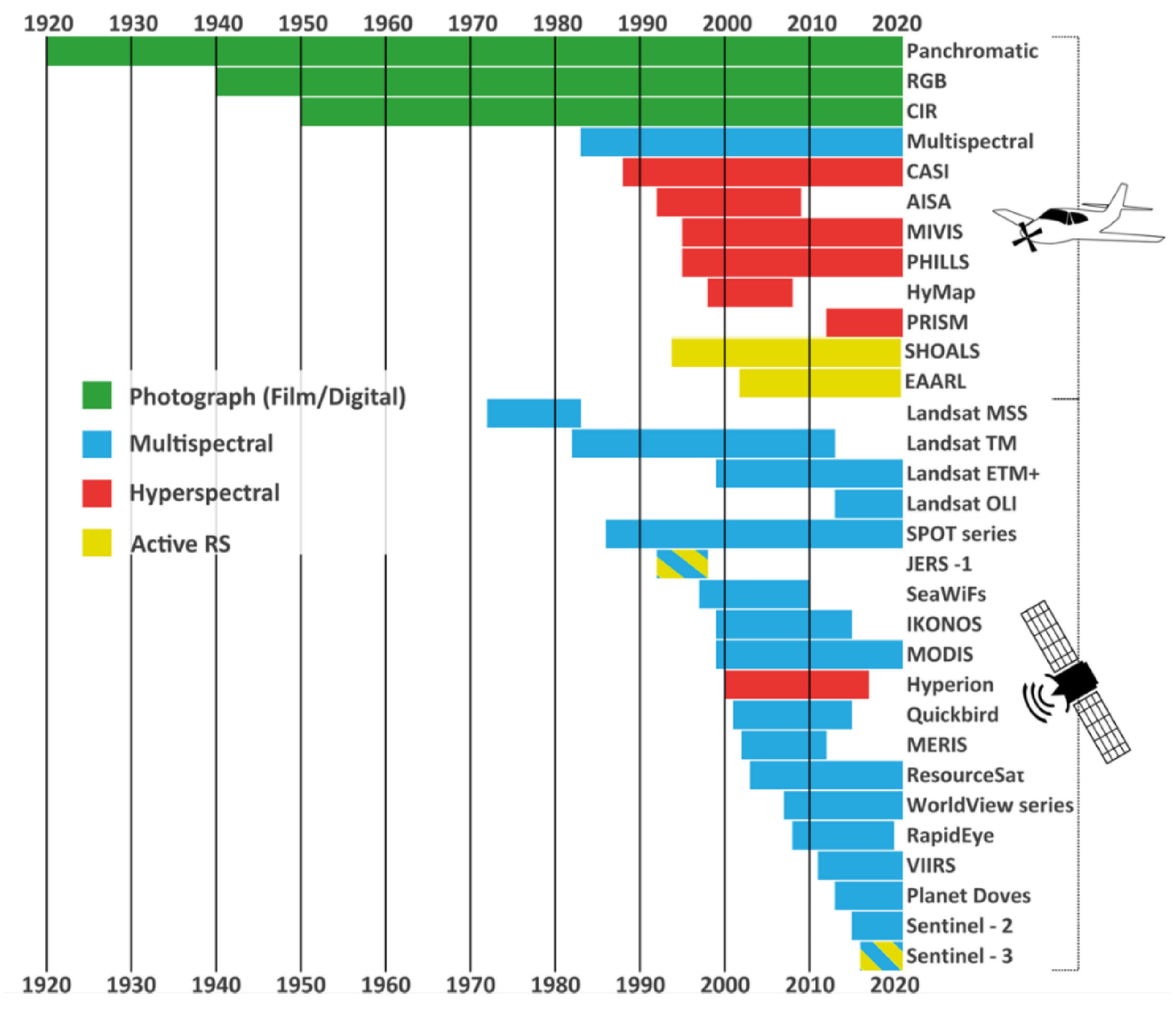
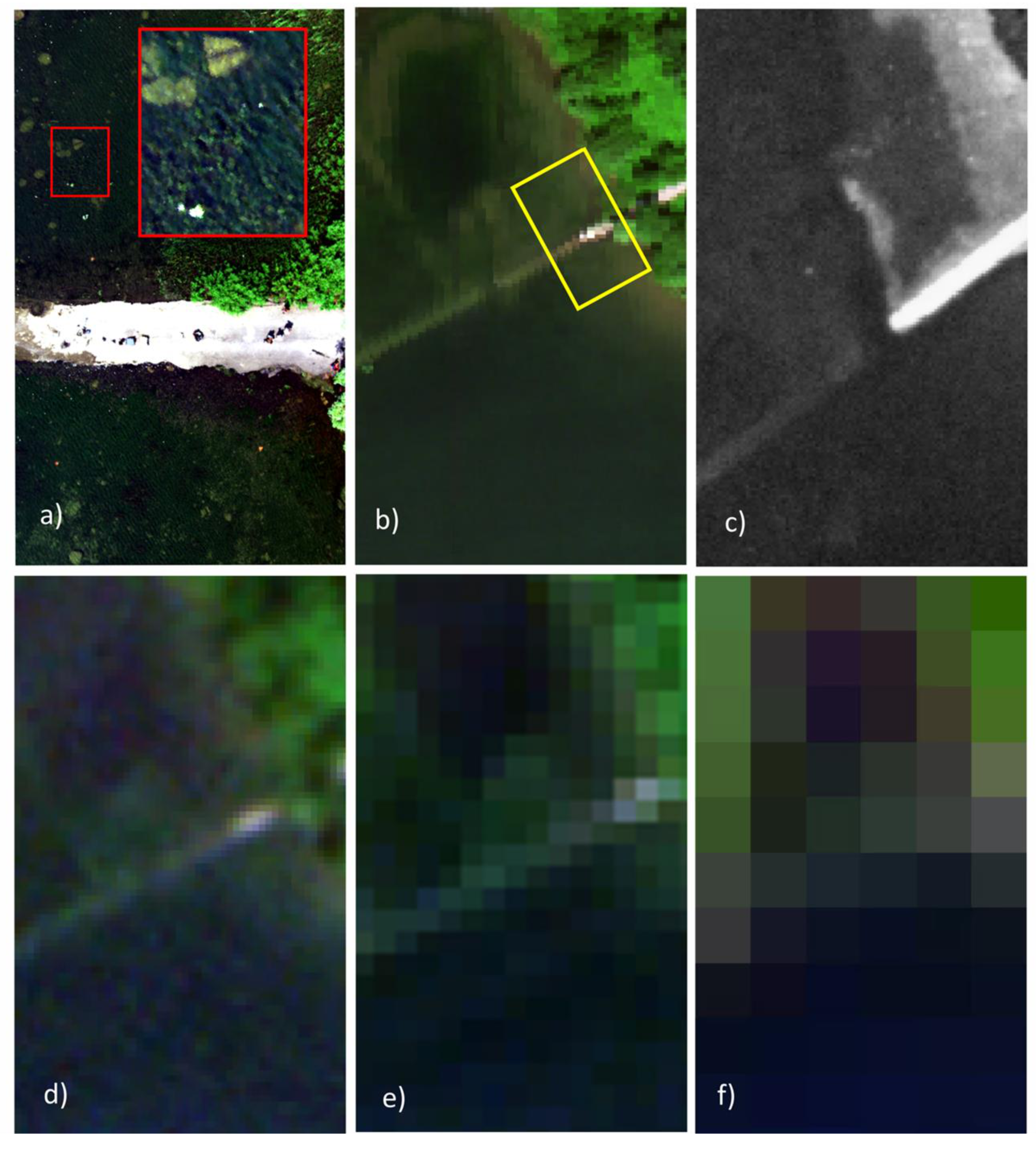
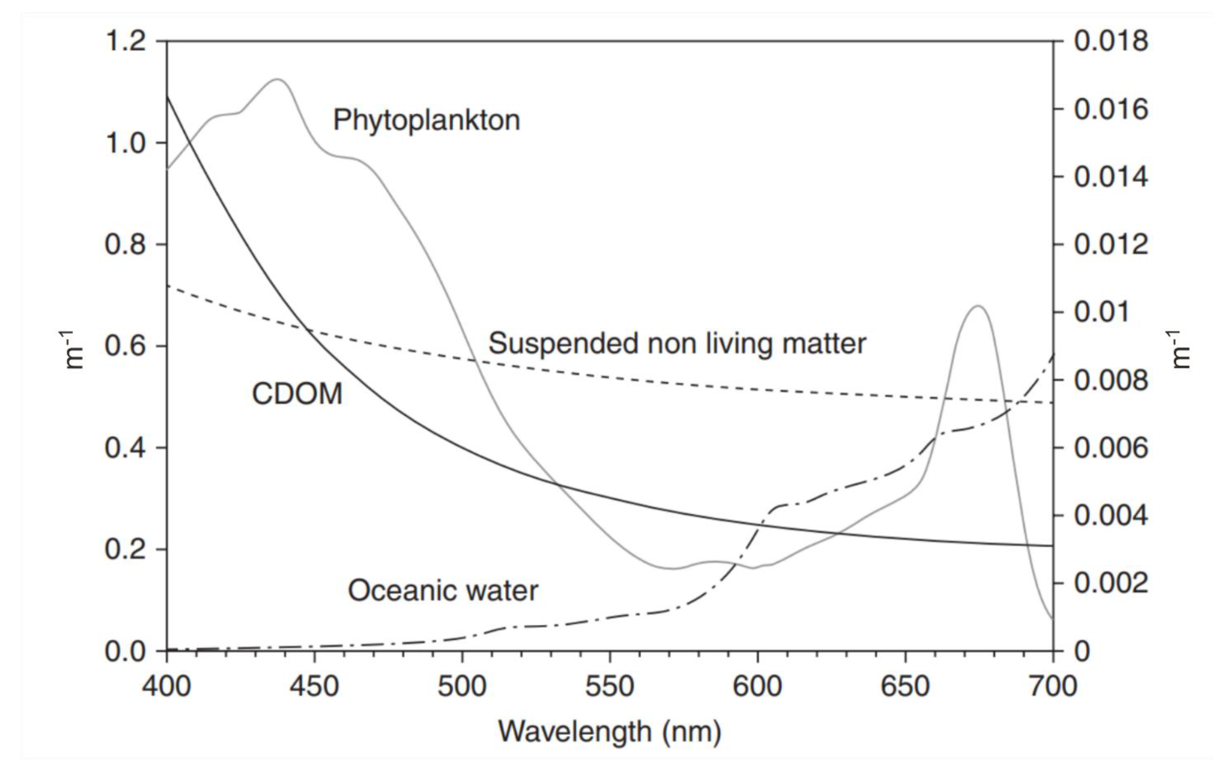
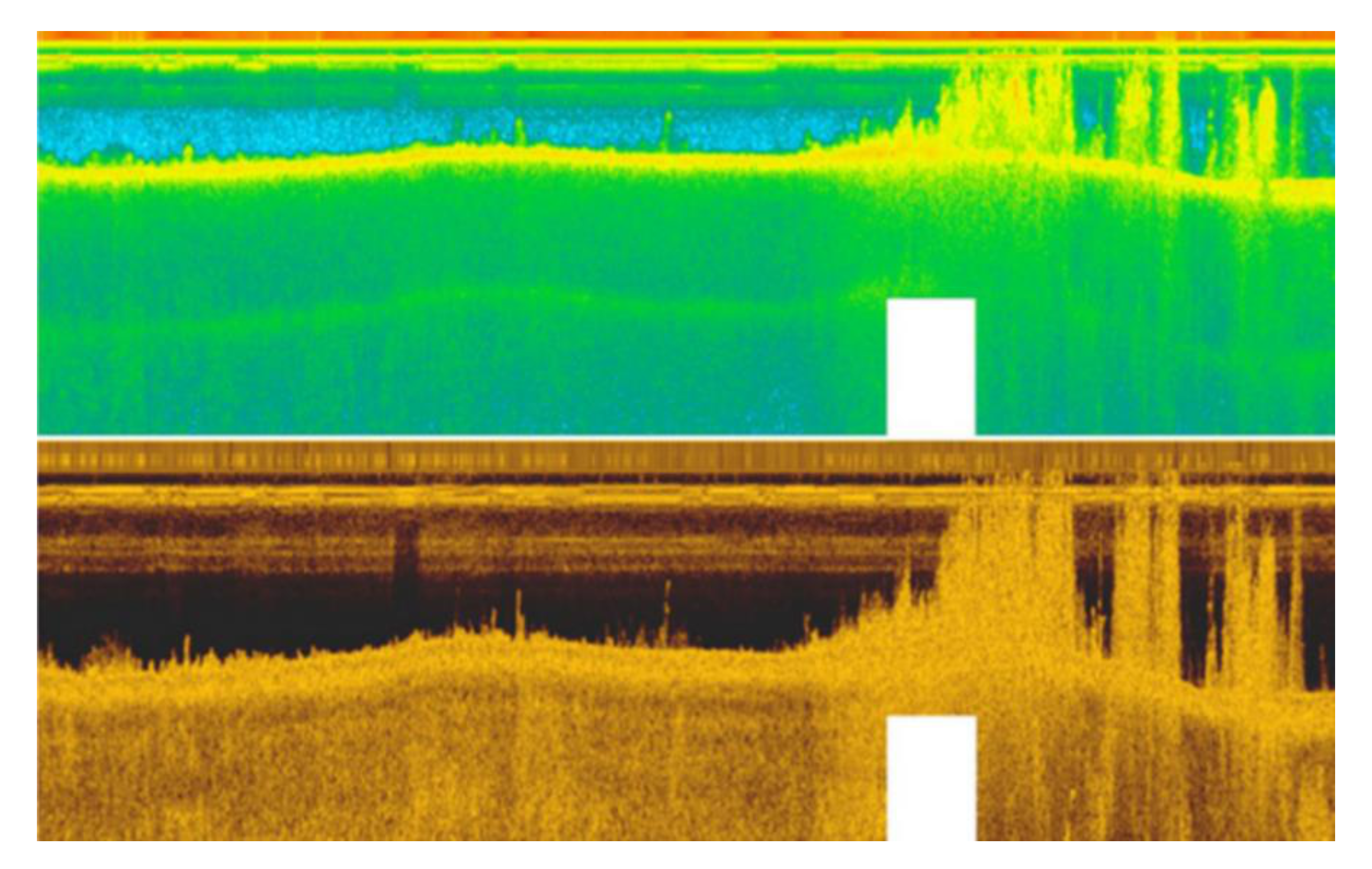
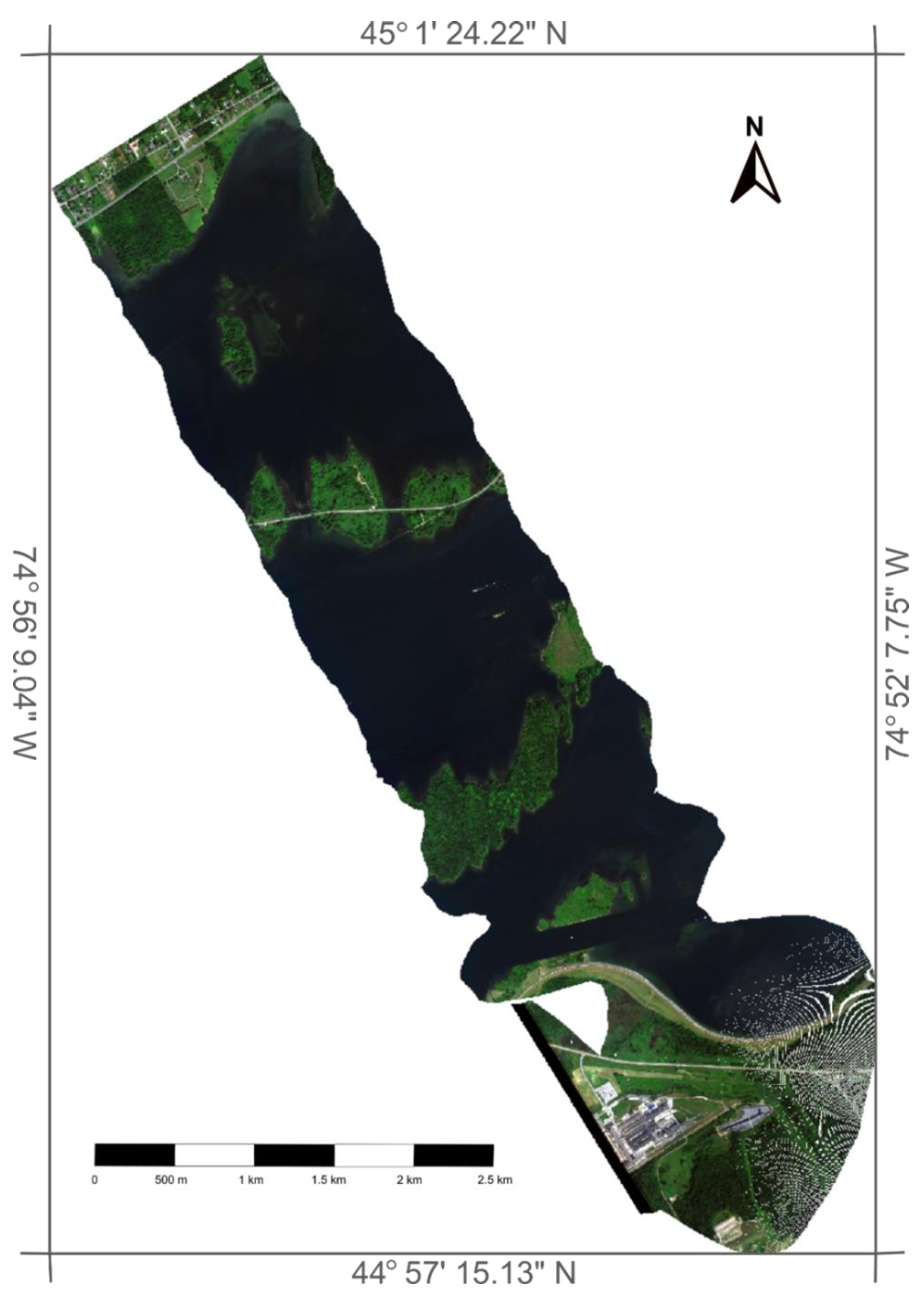
Figure 1. Operation chronology of a selection of remote sensors used in Submerged Aquatic Vegetation (SAV) research by platform and sensor type.
Remotesensing 13 00623 g001
Figure 2. Comparison of spatial resolutions in representing natural and man-made features (most notably a flooded road) in the Saint-Lawrence River, Ontario, Canada. (a) 3 cm resampled pixel size image acquired from an unmanned aerial vehicle (UAV) platform with the uCASI sensor (288 spectral bands). Subset is shown as a true color composite R:648 nm/G:548 nm/B:449 nm. (b) 1 m resampled pixel size image acquired from an airborne hyperspectral platform (CASI-1500, 288 spectral bands) Subset is shown as a true color composite R:641 nm/G:550 nm/B:471 nm. The yellow box indicates the spatial extent of frame (a). (c) Panchromatic film photograph from a KH-9 satellite taken in 1980 at a spatial resolution of 2 to 4 feet. (d) 3 m resampled pixel size image from the commercial PlanetScope satellite constellation (Dove-PS CubeSat). (e) 10 m resampled pixel size Sentinel-2 satellite image. (f) 30 m resampled pixel size Landsat image. For d-f, the respective RGB bands are displayed as true color composites.
Remotesensing 13 00623 g002
Figure 3. A simplified illustration of the interactions of light as they originate from the sun and are recorded by an optical sensor. The labels are as follows: LT = Radiance reflected by the target; LTS = Radiance reflected by the target then scattered out of the path to the sensor; LS = Radiance reflected by the non-target substrate; LA = Radiance reflected by the atmosphere to the sensor (also referred to as path radiance); LAS = Radiance scattered by the atmosphere; LW = Radiance reflected by the water column into the sensor; LWS = Radiance scattered by the water column; LWA = Radiance absorbed by the water column; LI = Radiance reflected by the air-water interface; LE = Radiance that is scattered into the scene by the ambient environment.
Remotesensing 13 00623 g003
Figure 4. The attenuative effect of the water column on the recorded signals of a flooded cement road at the Long Sault Parkway, ON, from airborne hyperspectral imagery (HSI) (CASI-1500). The colored boxes identify the pixels for which the spectra are shown on the right in units of radiance. The pixels chosen represent an increasing effect of the water column, with the dry road pixel being entirely unaffected by water. The inset photo shows what the flooded road looks like from the ground and was taken at the point indicated by the yellow circle. Note that the spectra here are in radiance, prior to atmospheric correction, as such the strong atmospheric water absorption features (e.g., 940 nm) can be seen in the spectrum from the dry road.
Remotesensing 13 00623 g004
Figure 5. The absorption profiles of four major constituents of natural waters. “Oceanic water” refers to very clear seawater. Colored Dissolved Organic matter (CDOM), oceanic water and suspended non-living matter all use the primary axis; only the phytoplankton spectrum uses the secondary axis. Reprinted from Subsea Optics and Imaging, Johnsen et al., Underwater hyperspectral imagery to create biogeochemical maps of seafloor properties, 508-535. Copyright (2013), with permission from Elsevier [52].
Remotesensing 13 00623 g005
Figure 6. Examples of vegetation spectra, with one standard deviation from the mean shown as shading; (a) A comparison of the effect of a thin layer of water (<5 mm) on the measured reflectance of a single species and the difference in profile shape between species. Note the prominent green peak in the spectrum of Nymod near 550 nm and the red-edge around 680 nm. The measured spectra of the submerged plants are lower across the spectrum, especially so in the NIR region. Valam does not display as prominent a green peak due to its higher relative concentration of accessory pigments making the leaves appear reddish-brown. (b) A comparison of the effect of epibiont and sediment fouling on the same plant sample. The profile of the fouled plant has a different shape and less spectral variability in the visible region than that of the unfouled plant. Nymod = Nymphaea odorata; Valam = Vallisnaria americana.
Remotesensing 13 00623 g006
Figure 7. Output from a single beam echosounder at 200 kHz (upper panel) and 800 kHz (lower panel) wave frequency. Macrophyte presence is identified by the areas of signal reflections (in the upper right hand of each panel) above the lake bottom. From Stocks et al., 2019 used according to CC-BY-ND http://creativecommons.org/licenses/by-nd/4.0/. Accessed on 7 October 2020 [33].
Remotesensing 13 00623 g007
Figure 8. The three methods used to acquire geolocational data in RS using UAVs and manned aircraft (labeled “platform” in the figure). (a) Platform location is determined using trilateration of three or more satellite signals. (b) Platform location is determined by the user applying a correction to the Global Navigation Satellite System (GNSS) receiver-generated location file. The correction file is downloaded from either a local base station operated by the user or from a commercial base station operated by external parties, such as governments. (c) Platform location is determined by applying a correction signal from a base station concurrently to data acquisition.
Remotesensing 13 00623 g008
Figure 9. The effect of platform attitude on the look direction of a sensor. (a) A “rolled” aircraft will cause a sensor to image an area adjacent to the intended flight line. (b) A change in platform pitch will cause the sensor to image a portion of the flight line that is not directly below it; rapid changes in pitch may therefore cause duplicate imaging of some targets (downward pitch aiming the sensor backward) or gaps (upward pitch aiming the sensor ahead). (c) A change in yaw will angle the view of the sensor so consecutive rows of pixels are not parallel, resulting in gaps and duplication.
Remotesensing 13 00623 g009
Figure 10. An example of imagery collected by a CASI-1500 onboard a manned aircraft acquiring imagery over the Long Sault Parkway, ON, Canada. Imagery was collected by a twin otter aircraft in partnership with the National Research Council of Canada. The NoData artefacts during the turn are portions of the ground over which no pixels are resolved in the geocorrection.
Remotesensing 13 00623 g010
Figure 11. An illustration of the extent and accuracy of previous aquatic RS work regarding SAV. The maximum accuracy found (reported as percent overall accuracy or R2) is depicted for each sensor-application pairing. Colored squares are on a gradient scale from 0 to 100, representing either percent overall accuracy or R2 × 100. White squares indicate that the sensor-application pair was encountered but no suitable overall accuracy measure was provided. Grey squares indicate that no source employed that sensor-application pairing. The large number of white and grey squares respectively demonstrate the need for consistent accuracy reporting and the huge research gaps to date in aquatic RS. Active sensors are italicized. All sources cited in this text were reviewed in the compilation of the figure, as well as references [140,141,142,143,144,145,146,147,148,149,150,151,152,153,154,155,156,157,158,159,160,161,162,163,164,165,166,167,168,169,170,171,172,173,174,175,176,177,178,179,180,181,182,183,184,185,186,187,188,189,190,191,192,193,194,195,196,197,198,199,200,201,202,203,204,205,206,207,208,209,210,211,212,213,214,215,216,217,218,219,220,221,222,223,224,225,226,227,228,229,230,231,232,233,234,235,236,237,238,239,240,241,242,243,244,245,246,247,248,249,250,251,252,253,254,255,256,257].
Remotesensing 13 00623 g011
Figure 12. The relationship between data complexity, training set size and mean classification accuracy. Complexity is here calculated as the number of bands raised to the exponent of the number of possible DN values per band (2# of bits). For HSI (and MSI with many bands), huge training sets would be required to obtain adequate classification accuracies if all bands are used. m = training set size. © 2002 IEEE. Reprinted, with permission, from Landgrebe, D. (2002), Hyperspectral image data analysis, IEEE Signal Processing Magazine [286].
Remotesensing 13 00623 g012
Figure 13. A simplified illustration of the principle of Structure-from-Motion Multiview Stereo photogrammetry. Common points at the corners of a rectangular prism seen from various angles are used to reconstruct a three-dimensional representation of the object. (a) the side; (b) the top; (c) the front; (d) the reconstructed rectangular prism. In reality, hundreds to thousands of key points (uniquely identified points) per photograph are needed with hundreds to thousands of matches between photographs to reconstruct a surface in 3D.
Remotesensing 13 00623 g013
Figure 14. Dense 3D point cloud from the Salobra river, Mato Grosso do Sul, Brazil generated through a Structure-from-Motion Multiview Stereo workflow from 768 UAV photographs. Photographs were acquired with a DJI Mavic 2 Pro UAV with an integrated Hasselblad L1D-2C camera. The camera has a 1” sensor (77° field of view) producing an image size of 5472 × 3648 pixels. A median of 67,753 key points were found per photograph with a median of 13,416 matches per photograph. Final ground sampling distance of the model is 1.2 cm. Extensive floating water hyacinth (Eichhornia crassipes) can be seen. The interactive point cloud can be accessed at https://bit.ly/waterhyacinth3D. Panel A (yellow) illustrates a shallow (<30 cm) area with several species of SAV which produce a habitat utilized by small characins. Panel B (blue) illustrates floating E. crassipes in deep (>2 m) water frequented by giant otters (Pteronura brasiliensis) and caimans (Caiman yacare). Panel C (purple) is a mid-range depth (1–2 m) with large patches of algae on the substrate. This open water habitat is frequented by larger fish species such as Prochilodus lineatus. Panel D (red) shows a bed of Camboba sp. in deep water (>2 m). The dense stems provide habitat for species such as Pygocentrus nattereri and Serrasalmus maculatus.
Remotesensing 13 00623 g014
Table 1. A list of essential remote sensing concepts mentioned in this study that researchers new to remote sensing (RS) should familiarize themselves with. Readers are directed to explanatory resources such as [37,38,39] for further detail.
ConceptDefinition
Acoustic remote sensingMeasures backscatter of acoustic waves which are vibrations of the medium (e.g., water) through which the waves propagate.
Active sensorA sensor that generates its own signal to illuminate the target.
Anomaly detectionA type of target detection in which there is no a priori target information.
ClassificationAn analytical method in which pixels in an image are given a thematic label as belonging to groups that have either been defined by the user or algorithmically generated.
Full-Width-Half-Maximum (FWHM)The width at half of the peak transmittance of the weighting function that describes the range of wavelengths a particular band is sensitive to. If a sensor has bands with narrow FWHMs finer spectral details can be resolved. For example, the uCASI (Figure 2a) has a narrow FWHM for each band (i.e., 2.6 nm) in contrast to 66 nm for band 2 of Sentinel-2.
Near Infrared (NIR)The region of the electromagnetic spectrum between 700 nm and 1100 nm.
Optical remote sensingMeasures reflected electromagnetic radiation.
Passive sensorA sensor that measures ambient energy, usually reflected solar radiation, thermal radiation, or microwaves.
Pixel sizeThe distance between pixels. It encompasses most of the area on the ground contributing signal to a pixel. Most often this metric is used to describe an image after it has been geometrically corrected to square pixels but can also refer to the raw unaltered geometry (see [40] for an example).
Radiometric resolutionDistinct levels into which the incoming signal is divided, the number of which determines how many energy intensity levels can be distinguished as being different by the sensor. This is typically given in the form of bits used to encode the pixel values in binary format where each bit corresponds to an exponent of 2 (e.g., an 8-bit image has 28 or 256 digital numbers referred to as grey levels). Many modern imagers acquire data in 10, 12 or 14-bits.
Spatial resolutionThe smallest resolvable detail achievable by a given system configuration. Spatial resolution can be divided as: very high < 1 m; high 1 m < x < 5 m; moderate 5 m < x < 30 m; low > 30 m.
Spectral profile/signature Response of a sensor to radiation across wavelengths sensed. Often represented as a curve of radiation reflected by a target.
Spectral resolutionAbility of a sensor to define fine wavelength intervals. A finer spectral resolution allows for a narrower wavelength range for a particular band. While the number of bands recorded by a given sensor can range from < 10 to > 200, the narrowness of the spectral interval that can be resolved defines the resolution. This is often reported as the FWHM of the spectral response function of each band.
Target detectionAn analysis method in which the known spectral, thermal, or microwave response of a material is located in an image.
Temporal resolutionThe time interval between successive measurements of the same target.
Ultra-violet (UV)The region of the electromagnetic spectrum between 270 nm and 400 nm.
Visible spectrum (VIS)The region of the electromagnetic spectrum between 400 nm to 700 nm comprising all visible wavelengths of light.
Table 2. The types of remote sensors that have been commonly applied to the study and monitoring of SAV, categorized by type, energy measured and number of bands (n). Example sensors and sources detailing applications of these sensors are also listed.
TypeEnergynNameDescriptionExamplesSources
ActiveAcoustic1Side-scan sonarEmits energy from above, at or near the water’s surface.Hummingbird SSS[33,69,70]
Acoustic1–2Echo-sounderEmits energy horizontally from within the water column.DIDSON, DT- X,
Sonic2024
[33,62,71,72]
Electro-
magnetic
1Bathymetric LiDAREmits green light (~530 nm) that penetrates the water column.SHOALS, EAARL[73,74]
PassiveElectro-
magnetic
1PanchromaticFilm and digital sensors that are sensitive to a wide wavelength range of light (usually the VIS) and produce greyscale images comprised of a single band.Film,
PAN band on SPOT
[75,76]
3Red-Green-Blue (RGB)Film and digital sensors that capture visible light to produce true color images.DSLR camera,
Go Pro
[77,78,79]
4–30MultispectralSensors that record up to 15 non-contiguous bands, potentially across the entire reflective optical spectrum.Sequoia sensor,
MEIS,
Landsat
[80,81,82]
30+HyperspectralSensors that record dozens to > 100 narrow, contiguous bands.ASD fieldspec,
CASI,
Hyperion
[43,83,84]
Table 3. A selection of SVIs of interest in SAV studies, whether due to their popularity, target material or use. Their full names, abbreviations, equations and sources that use each are listed. L represents a water column correction factor determined for a specific image.
NameAbbreviationEquationSource(s)
Normalized difference vegetation indexNDVI N I R   b a n d     r e d   b a n d N I R   b a n d   +   r e d   b a n d [21,294,295,296]
Normalized difference aquatic vegetation indexNDAVI N I R   b a n d     b l u e   b a n d N I R   b a n d   +   b l u e   b a n d [295,297,298]
Water-adjusted vegetation indexWAVI 1 + L N I R   b a n d     r e d   b a n d N I R   b a n d   +   r e d   b a n d [295,297,298]
Green-red vegetation indexGRVI g r e e n   b a n d     r e d   b a n d g r e e n   b a n d   +   r e d   b a n d [294]
Normalized total pigment to Chl-a ratio indexNPCI r e d   b a n d     b l u e   b a n d r e d   b a n d   +   b l u e   b a n d [299]
Publisher’s Note: MDPI stays neutral with regard to jurisdictional claims in published maps and institutional affiliations.

