
High Chlorophyll-a Areas along the Western Coast of South Sulawesi-Indonesia during the Rainy Season Revealed by Satellite Data

 , , ,
, , , 
Abstract
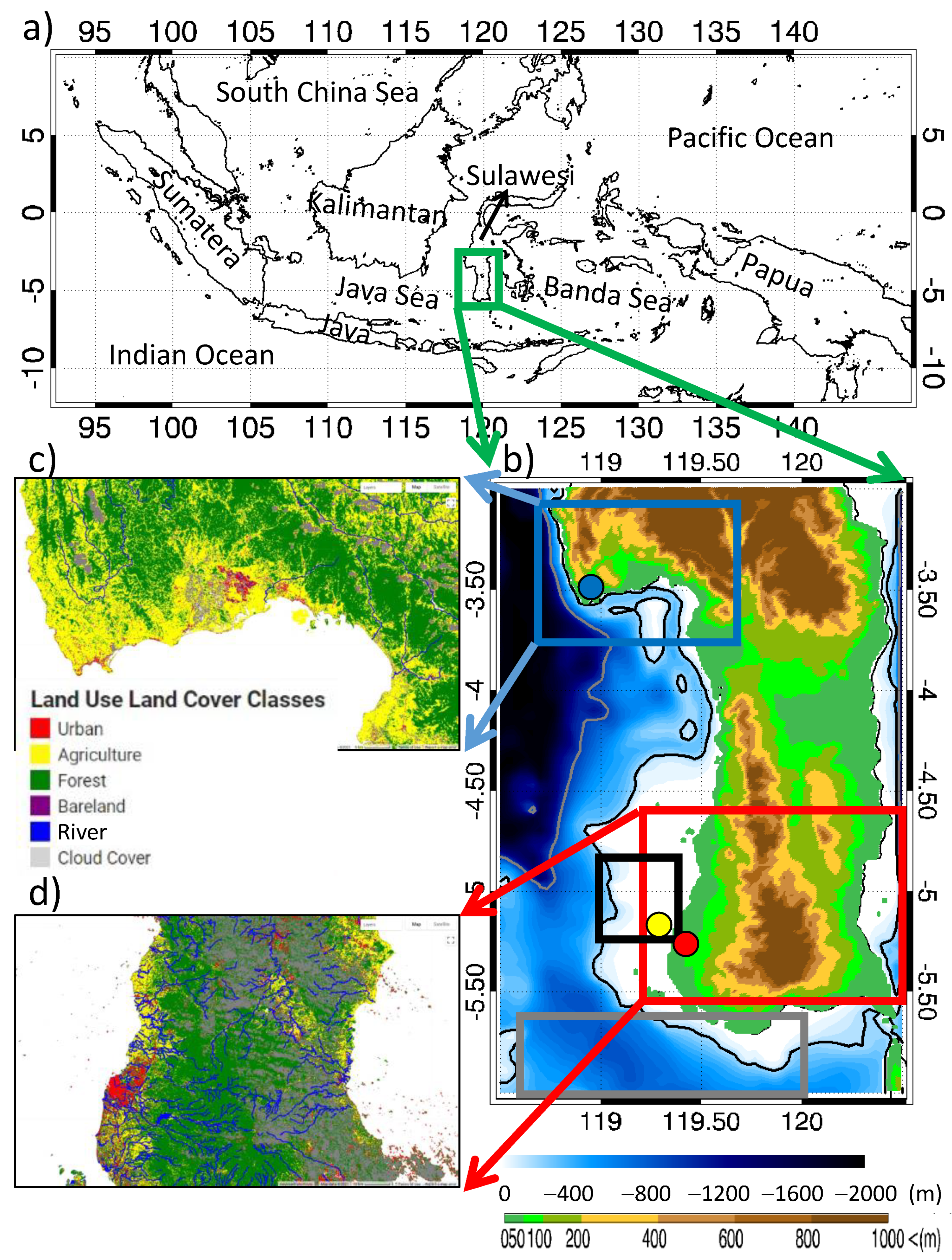
:1. Introduction
2. Dataset and Methods
2.1. Data
2.2. Method
3. Results
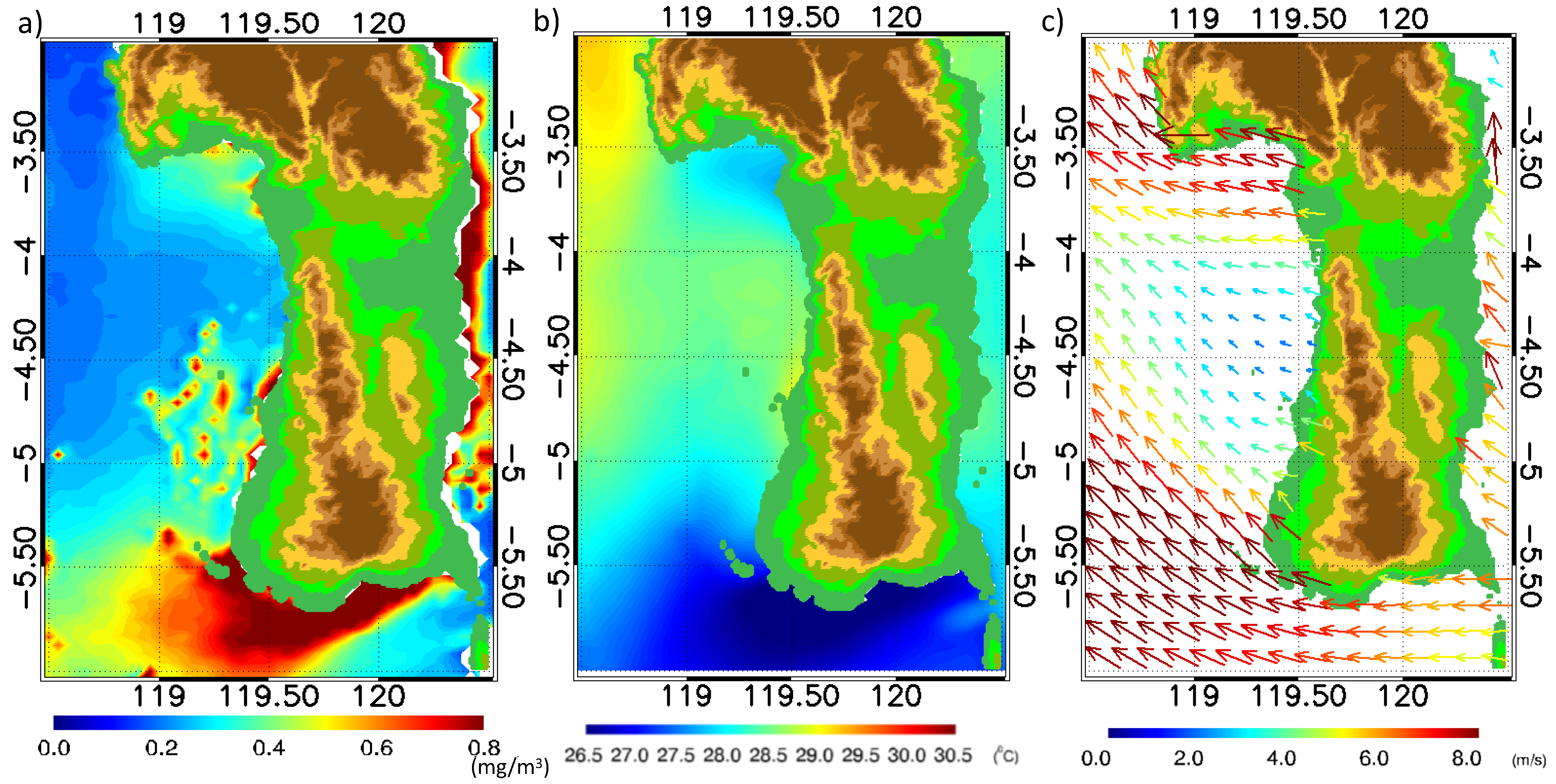
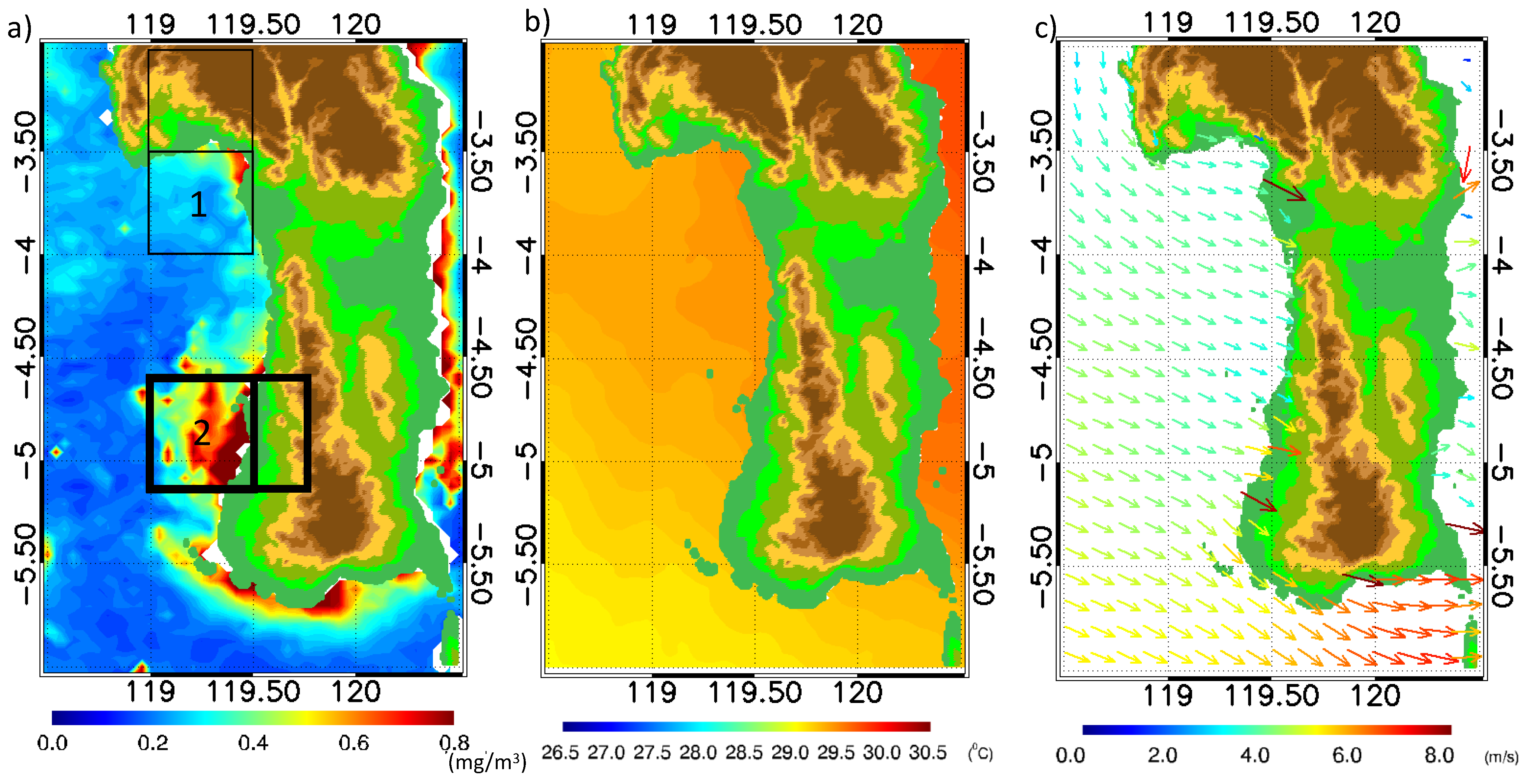
3.1. Spatial Distribution of Chl-a, SST, and Surface Wind
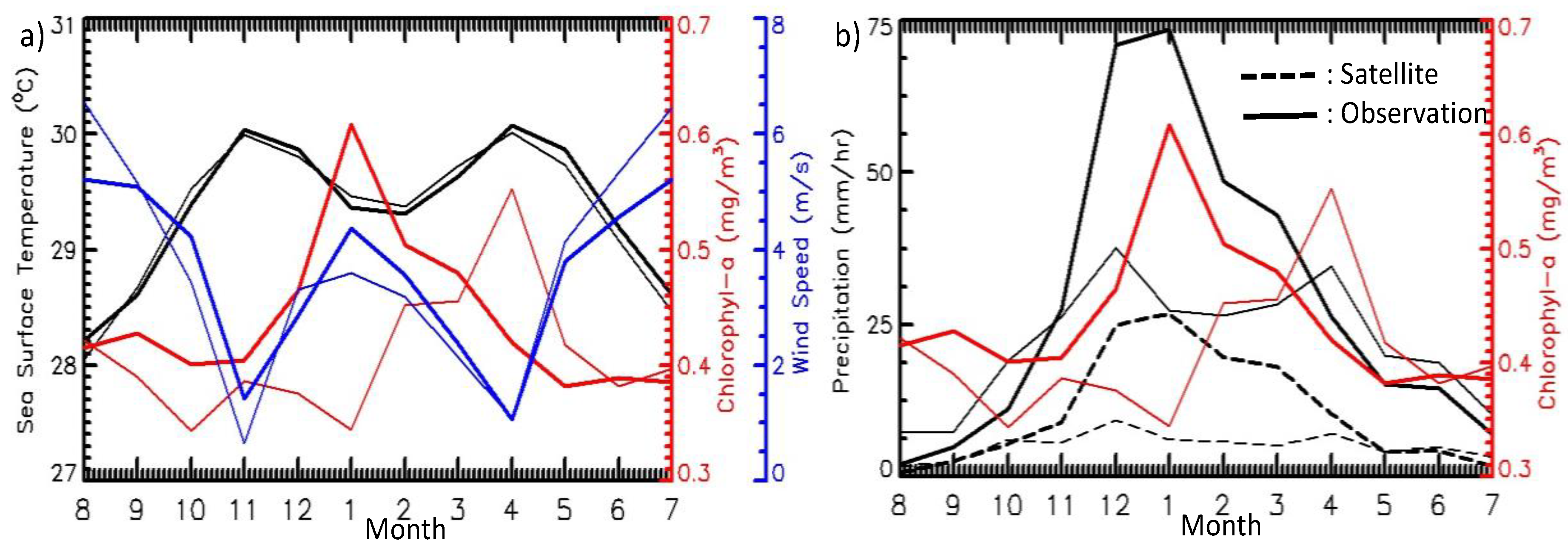
3.2. Temporal Analysis of Chl-a, SST, Surface Wind, and Precipitation
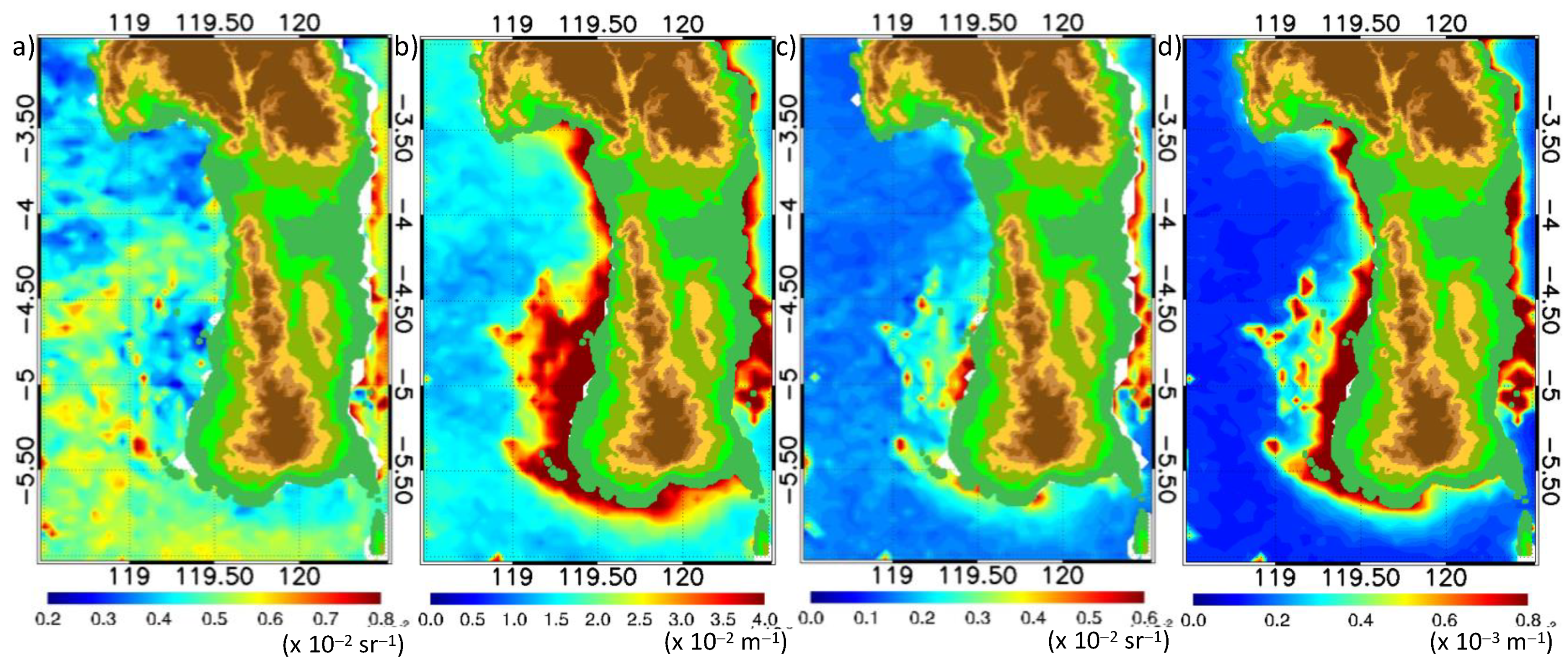
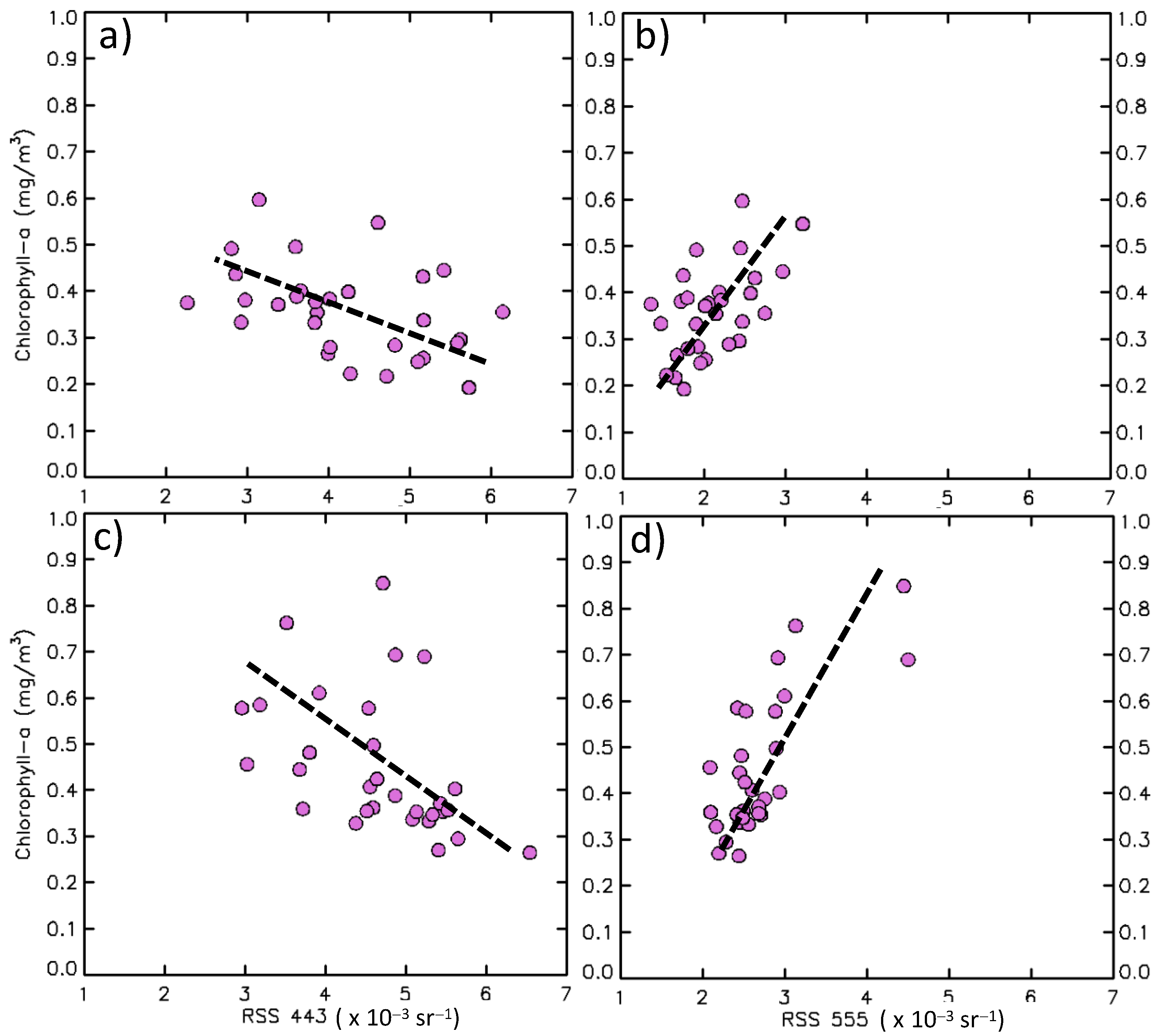
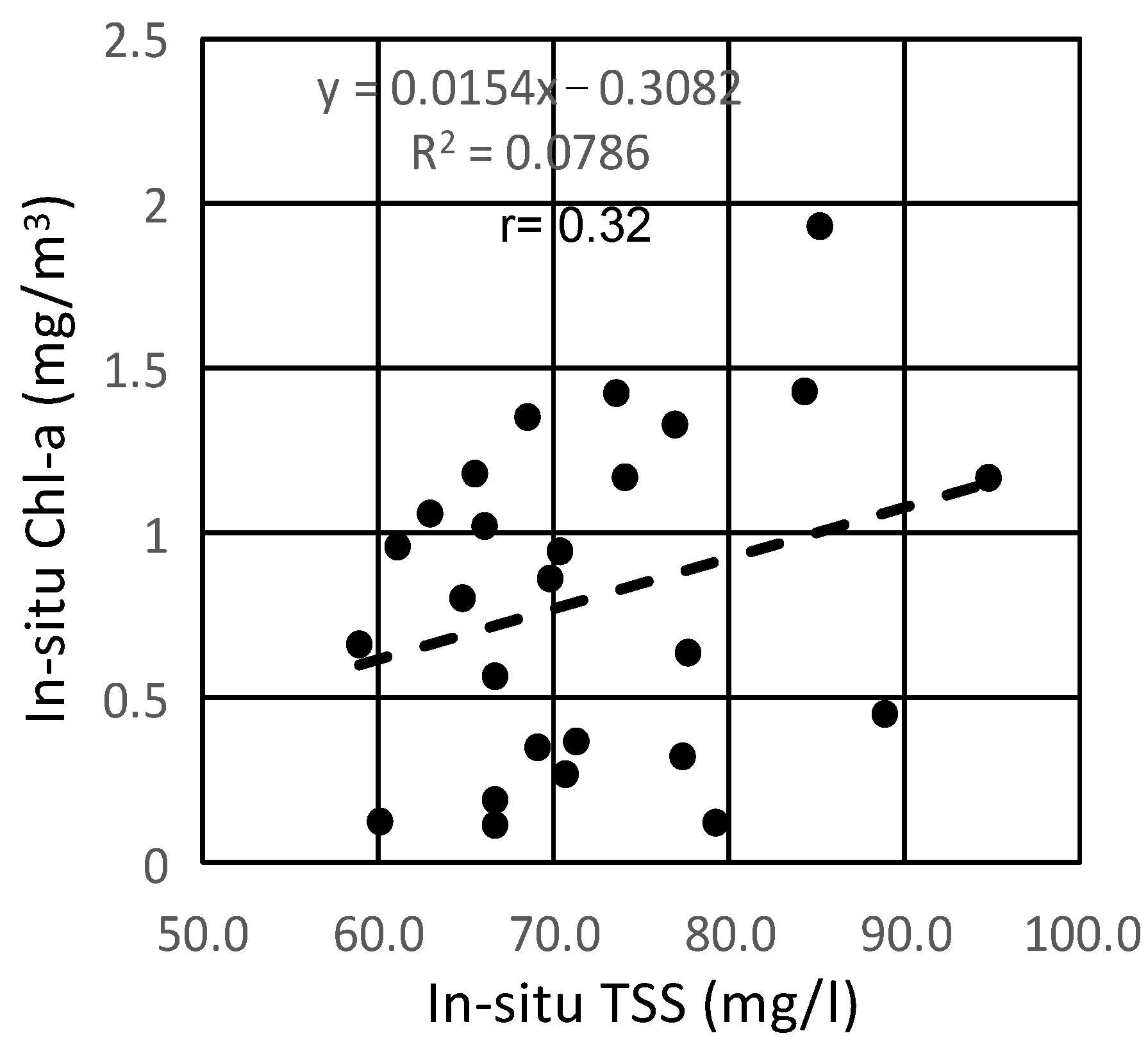
3.3. Possibility of Suspended Sediment that Bias the Observed Chl-a Concentration
4. Discussion
5. Conclusions
Author Contributions
Funding
Acknowledgments
Conflicts of Interest
References
- Welliken, M.A.; Melmambessy, E.H.P.; Merly, S.L.; Pangaribuan, R.D.; Lantang, B.; Hutabarat, J.; Wirasatriya, A. Variability Chlorophyll-a And Sea Surface Temperature As The Fishing Ground Basis Of Mackerel Fish In The Arafura Sea. In Proceedings of the 3rd International Conference on Energy, Environmental and Information System (ICENIS), Semarang, Indonesia, 14–15 August 2018; Volume 73, p. 4004. [Google Scholar] [CrossRef] [Green Version]
- Welliken, K.M.A.; Melmambessy, E.H.P.; Jumsar. Variability of Chlorophyll-a and Sea Surface Temperature, the effect on the Catches of Cakalang Fish in Sawu Sea of East Nusa Tenggara. Int. J. Civ. Eng. Technol. 2019, 10, 715–723. [Google Scholar]
- Lahlali, H.; Wirasatriya, A.; Gensac, A.E.; Helmi, M.; Kunarso; Kismawardhani, R.A. Environmental aspects of tuna catches in the Indian Ocean, southern coast of Java, based on satellite measurements. In Proceedings of the 4th International Symposium on Geoinformatics 2018, Malang, Indonesia, 10–12 November 2018; pp. 1–6. [Google Scholar] [CrossRef]
- Siswanto, E.; Horii, T.; Iskandar, I.; Gaol, J.L.; Setiawan, R.Y.; Susanto, R.D. Impacts of climate changes on the phytoplankton biomass of the Indonesian Maritime Continent. J. Mar. Syst. 2020, 212, 103451. [Google Scholar] [CrossRef]
- Setiawan, R.Y.; Kawamura, H. Summertime Phytoplankton Bloom in the south Sulawesi Sea. IEEE J. Sel. Top. Appl. Earth Observ. Remote Sens. 2011, 4, 241–244. [Google Scholar] [CrossRef]
- Utama, F.G.; Atmadipoera, A.S.; Purba, M.; Sudjono, E.H.; Zuraida, R. Analysis of upwelling event in Southern Makassar Strait. IOP Conf. Ser. Earth Environ. Sci. 2017, 54, 12085. [Google Scholar] [CrossRef] [Green Version]
- Nurdin, S.; Mustapha, M.A.; Lihan, T. The relationship between sea surface temperature and chlorophyll-a concentration in fisheries aggregation area in the archipelagic waters of Spermonde using satellite images. In AIP Conference Proceedings; American Institute of Physics: University Park, MD, USA, 2013; Volume 1571, p. 466. [Google Scholar] [CrossRef]
- Nurdin, S.; Mustapha, M.A.; Lihan, T.; Zainuddin, M. Applicability of remote sensing oceanographic data in the detection of potential fishing grounds of Rastrelliger kanagurta in the archipelagic waters of Spermonde, Indonesia. Fish. Res. 2017, 196, 1–12. [Google Scholar] [CrossRef]
- Sathyendranath, S.; Brewin, R.J.W.; Brockmann, C.; Brotas, V.; Calton, B.; Chuprin, A.; Cipollini, P.; Couto, A.B.; Dingle, J.; Doerffer, R.; et al. An ocean-colour time series for use in climate studies: The experience of the Ocean-Colour Climate Change Initiative (OC-CCI). Sensors 2019, 19, 4285. [Google Scholar] [CrossRef] [Green Version]
- Shi, W.; Wang, M. Observations of a Hurricane Katrina-induced phytoplankton bloom in the Gulf of Mexico. Geophys. Res. Lett. 2007, 34, L11607. [Google Scholar] [CrossRef]
- Zheng, G.M.; Tang, D.L. Offshore and nearshore chlorophyll increases induced by typhoon winds and subsequent terrestrial rainwater runoff. Mar. Ecol. Prog. Ser. 2007, 333, 61–74. [Google Scholar] [CrossRef] [Green Version]
- JPL MUR MEaSUREs Project. GHRSST Level 4 MUR Global Foundation Sea Surface Temperature Analysis. Ver. 4.1. PO.DAAC, CA, USA, 2015. Available online: https://doi.org/10.5067/GHGMR-4FJ04 (accessed on 25 October 2021).
- Chao, Y.; Li, Z.; Farrara, J.D.; Hung, P. Blending sea surface temperatures from multiple satellites and in situ observations for coastal oceans. J. Atmos. Ocean. Technol. 2009, 26, 1415–1426. [Google Scholar] [CrossRef]
- Liu, Y.; Weisberg, R.H.; Law, J.; Huang, B. Evaluation of Satellite-Derived SST Products in Identifying the Rapid Temperature Drop on the West Florida Shelf Associated with Hurricane Irma. Mar. Technol. Soc. J. 2018, 52, 43–50. [Google Scholar] [CrossRef]
- Figa-Saldaña, J.; Wilson, J.J.W.; Attema, E.; Gelsthorpe, R.V.; Drinkwater, M.R.; Stoffelen, A. The Advanced Scatterometer (ASCAT) on the Meteorological Operational (MetOp) Platform: A Follow on for European Wind Scatterometers. Can. J. Remote Sens. 2002, 28, 404–412. [Google Scholar] [CrossRef]
- Otsuka, S.; Kotsuki, S.; Miyoshi, T. Nowcasting with data assimilation: A case of Global Satellite Mapping of Precipitation. Weather Forecast. 2016, 31, 1409–1416. [Google Scholar] [CrossRef]
- Maslukah, L.; Setiawan, R.Y.; Nurdin, N.; Helmi, M.; Widiaratih, R. Phytoplankton Chlorophyll-a Biomass and the Relationship with Water Quality in Barrang Caddi, Spermonde, Indonesia. Ecol. Eng. Environ. Technol. 2021, in press. [Google Scholar] [CrossRef]
- Wirasatriya, A.; Setiawan, R.Y.; Subardjo, P. The effect of ENSO on the variability of chlorophyll-a and sea surface temperature in the Maluku Sea. IEEE J. Sel. Top. Appl. Earth Observ. Remote Sens. 2017, 10, 5513–5518. [Google Scholar] [CrossRef]
- Haack, T.; Burk, S.D.; Dorman, C.; Rogers, D. Supercritical flow interaction within the Cape Blanco–Cape Mendocino orographic complex. Mon. Weather Rev. 2001, 129, 688–708. [Google Scholar] [CrossRef]
- Shimada, T.; Sawada, M.; Sha, W.; Kawamura, H. Low-Level Easterly Winds Blowing through the Tsugaru Strait, Japan. Part I: Case Study and Statistical Characteristics Based on Observations. Mon. Weather Rev. 2010, 138, 3806–3821. [Google Scholar] [CrossRef]
- Wirasatriya, A.; Sugianto, D.N.; Helmi, M.; Setiawan, R.Y.; Koch, M. Distinct Characteristics of SST Variabilities in the Sulawesi Sea and the Northern Part of the Maluku Sea During the Southeast Monsoon. IEEE J. Sel. Top. Appl. Earth Observ. Remote Sens. 2019, 12, 1763–1770. [Google Scholar] [CrossRef]
- Wirasatriya, A.; Setiawan, J.D.; Sugianto, D.N.; Rosyadi, I.A.; Haryadi, H.; Winarso, G.; Setiawan, R.Y.; Susanto, R.D. Ekman dynamics variability along the southern coast of Java revealed by satellite data. Int. J. Remote Sens. 2020, 41, 8475–8496. [Google Scholar] [CrossRef]
- Maslukah, L.; Zainuri, M.; Wirasatriya, A.; Salma, U. Spatial Distribution of Chlorophyll-a and Its Relationship with Dissolved Inorganic Phosphate Influenced by Rivers in the North Coast of Java. J. Ecol. Eng. 2019, 20, 18–25. [Google Scholar] [CrossRef]
- Siswanto, E.; Tang, J.; Yamaguchi, H.; Ahn, Y.-H.; Ishizaka, J.; Yoo, S.; Kim, S.-W.; Kiyomoto, Y.; Yamada, K.; Chiang, C.; et al. Empirical ocean-color algorithms to retrieve chlorophyll-a, total suspended matter, and colored dissolved organic matter absorption coefficient in the Yellow and East China Seas. J. Oceanogr. 2011, 67, 627–650. [Google Scholar] [CrossRef]
- Wirasatriya, A.; Susanto, R.D.; Kunarso, K.; Jalil, A.R.; Ramdani, F.; Puryajati, A.D. Northwest monsoon upwelling within the Indonesian seas. Int. J. Remote Sens. 2021, 42, 5437–5458. [Google Scholar] [CrossRef]
- Maslukah, L.; Zainuri, M.; Wirasatriy, A.; Maisyarah, S. The Relationship among Dissolved Inorganic Phosphate, Particulate Inorganic Phosphate, and Chlorophyll-a in Different Seasons in the Coastal Seas of Semarang and Jepara. J. Ecol. Eng. 2020, 21, 135–142. [Google Scholar] [CrossRef]
- Setiawan, R.Y.; Habibi, A. Satellite Detection of Summer Chlorophyll-a Bloom in the Gulf of Tomini. IEEE J. Sel. Top. Appl. Earth Observ. Remote Sens. 2011, 4, 944–948. [Google Scholar] [CrossRef]
- Setiawan, R.Y.; Habibi, A. SST cooling in the Indonesian seas. Ilmu Kelaut. Indones. J. Mar. Sci. 2010, 15, 42–46. [Google Scholar] [CrossRef]

| Variable | SST | Chl-a | ||
|---|---|---|---|---|
| First Area | Second Area | First Area | Second Area | |
| Wind speed | −0.79 | −0.73 | 0.35 | 0.40 |
| Precipitation | 0.43 | 0.51 | ||
| Wind speed and precipitation | 0.46 | 0.58 | ||
Publisher’s Note: MDPI stays neutral with regard to jurisdictional claims in published maps and institutional affiliations. |
© 2021 by the authors. Licensee MDPI, Basel, Switzerland. This article is an open access article distributed under the terms and conditions of the Creative Commons Attribution (CC BY) license (https://creativecommons.org/licenses/by/4.0/).
Share and Cite
Wirasatriya, A.; Susanto, R.D.; Setiawan, J.D.; Ramdani, F.; Iskandar, I.; Jalil, A.R.; Puryajati, A.D.; Kunarso, K.; Maslukah, L. High Chlorophyll-a Areas along the Western Coast of South Sulawesi-Indonesia during the Rainy Season Revealed by Satellite Data. Remote Sens. 2021, 13, 4833. https://doi.org/10.3390/rs13234833
Wirasatriya A, Susanto RD, Setiawan JD, Ramdani F, Iskandar I, Jalil AR, Puryajati AD, Kunarso K, Maslukah L. High Chlorophyll-a Areas along the Western Coast of South Sulawesi-Indonesia during the Rainy Season Revealed by Satellite Data. Remote Sensing. 2021; 13(23):4833. https://doi.org/10.3390/rs13234833
Chicago/Turabian StyleWirasatriya, Anindya, Raden Dwi Susanto, Joga Dharma Setiawan, Fatwa Ramdani, Iskhaq Iskandar, Abd. Rasyid Jalil, Ardiansyah Desmont Puryajati, Kunarso Kunarso, and Lilik Maslukah. 2021. "High Chlorophyll-a Areas along the Western Coast of South Sulawesi-Indonesia during the Rainy Season Revealed by Satellite Data" Remote Sensing 13, no. 23: 4833. https://doi.org/10.3390/rs13234833
APA StyleWirasatriya, A., Susanto, R. D., Setiawan, J. D., Ramdani, F., Iskandar, I., Jalil, A. R., Puryajati, A. D., Kunarso, K., & Maslukah, L. (2021). High Chlorophyll-a Areas along the Western Coast of South Sulawesi-Indonesia during the Rainy Season Revealed by Satellite Data. Remote Sensing, 13(23), 4833. https://doi.org/10.3390/rs13234833